Aerodynamic Drag Coefficient Prediction of a Spike Blunt Body Based on K-Nearest Neighbors

Abstract

Spike blunt bodies are a method to reduce drag when a body moves at speeds above sound. Several numerical works based on computational fluid dynamics (CFD) have deeply studied fluid performance and highlighted its advantages. However, most documentation focuses on modifying spike physical properties while keeping constant supersonic or hypersonic flow conditions. In recent years, machine learning models have emerged as viable tools to predict values in almost any field, including aerodynamics. In the case of CFD, many models have been explored, such as support vector regression, ensemble methods, and artificial neural networks. However, a simple and easy-to-implement method such as k-Nearest Neighbors has not been extensively explored. This work extrapoled k-Nearest Neighbors to predict the drag coefficient of a spike blunt body for a range of supersonic and hypersonic speeds based on drag data obtained from CFD analysis. The parametric study of the spike blunt body was performed considering body diameter, spike length, and freestream Mach number as input variables. The algorithm presents proper predictions, with errors less than 5% for the drag coefficient and considering a minimum of three neighbor nodes. The k-NN was compared again Kriging model and k-NN presents a better accuracy. The above validates the flexibility of the method and shows a new area of opportunity for the calculation of aerodynamic properties.

1. Introduction

Drag, lift, and lateral forces emerge under external flow conditions [1]. If fluid flows move above the speed of sound, a detached shock wave is presented [2]. The sudden change in pressure produced by supersonic or hypersonic speeds can increase drag forces as well as heat; this phenomenon is focused in front of blunt bodies, e.g., missiles, space shuttles, and rockets [3,4,5]. In the case of aerodynamic response, streamlined bodies present better performance; however, blunt body shapes are preferred due to the available space inside of them [6].

Supersonic flow over a blunt body is characterized by a shock wave created over the body surface, propagating downstream. This phenomenon generates drag forces due to pressure differences and viscous effects. Moreover, it causes heat generation from gas compression at the shock wave front that could damage the body surface [7]. Several techniques have been proposed to control drag in blunt bodies under the supersonic regime, such as a geometrical change over the body by adding a spike. This spike is a protrusion that extends from the nose of the object and is commonly aligned to the direction flow [8]. Spikes create an oblique primary shock wave that reduces the strength of a secondary shock wave produced by the blunt body; thus, this decreases the amount of drag generated by the object [9]. The effectiveness of a spike decreasing drag depends on several factors, including angle of attack (AoA), spike length, Mach number, and blunt body shape [10,11,12]. It is important to comment that the sharp leading edge of the spike can be optimized to promote the desired shock wave pattern and, in consequence, reduce heat caused by shock wave concentration and keep stability at high speeds, as well as reduce drag generated by the remaining shock wave [8].

Major advances in the understanding of the use of the drag control mechanism by spikes have been produced through experimental and numerical studies, particularly through the CFD [13,14,15,16]. However, the fidelity of these works requires high computational resources and time, mainly when complex geometries or configurations are introduced. In computational fluid dynamics, accuracy and quick testing are key for new configurations; in this sense, it is evident to explore alternative approaches to accelerate the design process.

In recent years, machine learning (ML) has emerged as a promising complementary avenue with its capacity to learn from and make predictions on data. By harnessing versatile ML algorithms, attenuating the reliance on continuous CFD simulations is possible, thereby advancing a more efficient predictive framework for fluid flow phenomena and their effects, including aerodynamic properties. There are several articles that recognize the advantages and possibilities of machine learning [17,18]. Research areas of aeronautics [19,20], aeroacoustics [21,22,23], combustion, resistance of materials [24,25], and manufacturing have benefited from the application of unsupervised learning. Particularly on the prediction of aerodynamic coefficients using Neuronal Networks [26,27,28], there is the work of Linse and Stengel [26] applied to aircraft transport, with good results validated with flight-tested data in the early 90’s. The dynamic stall effect was performed by Suresh et al. [27] at a high angle of attack again with experimental data. Secco and Mattos [28] studied the aerodynamic response of transport airplanes. Using a broad dataset generated by CFD simulations, they trained a model and reduced by 4000 times the prediction of drag and lift coefficients. Recently, Ghoteyshi et al. [29], Wang et al. [30], and Hou et al. [31] successfully tested the viability of these tools.

Despite these promising methods, their implementation is often difficult due to the inherent complexities, such as the need for extensive hyperparameter tuning, large training datasets, and an advanced understanding of both the fluid mechanics and machine learning domains. In other words, accurate and accessible models to CFD practitioners without deep ML expertise are scarce. This gap beckons for a method that strikes a balance between predictive performance and ease of deployment. Among the many remarkable machine learning strategies, the k-Nearest Neighbors (k-NN) algorithm emerges as a robust predicting tool renowned for its simplicity and effectiveness [32]. The fidelity of this model is evidenced by its adaptability and scalability, with minimal need for retraining or extensive parameter adjustments.

Currently, to determine the drag coefficient for a spike blunt body, numerical simulations or experimental work must be conducted. Each new work could imply spike length modifications, spike geometrical changes, angles, or new flow characteristics. With the method presented in this document, it is possible to predict drag performance for a large range of Mach numbers for different geometrical configurations with a relatively small dataset. Despite previous works that have used CFD in combination with k-NN as a prediction mechanism, it has not been deeply explored in supersonic flow ranges or applied to spike blunt bodies.

The rest of the paper is presented as follows: Methodology, Prototype Geometry, Numerical Simulation, Validation and Dataset Generation, Results and Discussion, and Conclusions.

2. Method

This section describes the necessary steps to test the effectiveness of the k-NN algorithm to calculate the drag coefficient of a spike blunt body, as well as the implementation of the calculation technique. A reliable and complete dataset is essential to providing information to the ML algorithm. To obtain the drag coefficient using CFD, the continuity, momentum, and energy equations were solved using the FloWorks package provided in SolidWorks 2023 CAD software. These equations are solved in a cartesian frame using the Finite Volume Method (FVM). Further details on their numerical implementation can be found in [33]. It is important to point out that this solver is based upon the use of structured cartesian meshes. Hence, the blunt body and spike were modeled by means of the cut-cell method [34]; this approach allows the mesh to be independent of the geometry. Additionally, turbulent behavior was modeled by the Reynolds-averaged Navier–Stokes (RANS) approach using the modified two-equation turbulence model k–ε, which implements the Lam and Bremhorst damping function to solve the laminar, turbulent, and transitional flows of homogeneous fluids. Once the dataset is determined, the k-NN algorithm of the Machine Learning Technique is applied.

2.1. Numerical Simulation and Validation

Solidworks flow simulation is used in this work to analyze a spike blunt body immersed in compressible flow. To validate the effectiveness along a wide range of Mach numbers, a sphere geometry was selected, and several works report drag coefficient performance since subsonic to supersonic flow conditions [35,36]. An independent mesh study was carried out, firstly, orthogonal meshes with different refinement levels, a fine one (553,776 cells) and a coarse one (144,952 cells). Secondly, an adaptive mesh is considered (two refinement levels). Then, the external flow on the sphere is considered the baseline case for the validation of the code. The sphere and blunt body are analyzed at the same thermal conditions; see

Table 1. Thermal and transport properties.

Pressure (P, atm)	Temperature (T, K)	Viscosity (μ, Pa·s)	Density (ρ, kg/m3)	Gas Constant (Rg, kJ/kg·K)	Speed of Sound (c, m/s)
1.0	290	1.8 × 10−5	0.816	0.287	340

.

The computational domain is nearly identical to the spike blunt body; see Section 2.2. The validation code is performed with a smooth sphere for different Mach numbers ranging from 0.9 to 6.0. The variances between results obtained with the fine and coarse grids are less than 5% but with relative errors slightly higher than 10% with regard to the experimental and numerical results of the drag coefficient of a sphere. The adaptive mesh of 2 levels shows slightly better performance in comparison with other mesh grids. All of them show relative errors below 9% in the whole range of a Mach number. However, adaptative mesh time simulation is considerably higher than fine refinement; therefore, this one was selected for validation and dataset creation; see Figure 1. Overall, the results show good agreement with the experimental data.

2.2. Spike Blunt Body Prototype

As in Kalimuthu et al. [12], a flat-face spike blunt body is analyzed considering diameter (d) and length (l) and a blunt body diameter (D) of 1 inch; see Figure 2. These parameters are treated as dimensionless, as shown in the next section.

Once the numerical model has been validated and the geometry of interest is defined, it is possible to perform the simulations that supply the dataset of the machine learning algorithm.

The simulated prototype geometry is the simplest spike blunt bodies. A 3D and orthogonal Cartesian frame were considered in all simulations, Figure 3. The main flow moves positively and parallel to the x direction. Similar to the sphere, three orthogonal meshes were tested: a fine mesh with ≈6 × 10⁵ cells and a coarse one with ≈1.5 × 10^5, as well as an adaptive mesh with two refine levels. The finest mesh is used to develop all simulations to generate the drag coefficient dataset.

2.3. Dataset

As mentioned earlier, a reliable and complete dataset is essential to providing information to the ML algorithm. The predictions were developed over a wide range of Mach numbers, aspect ratios, and Reynolds. The dataset needed to feed the selected machine learning model was generated through sets of simulations based on Table 1 using SolidWorks Flow simulation. Overall, 239 simulations were considered (Appendix A). The dataset used in this work is built with simulation results of geometry dimensions described previously. Variables considered are force over x direction, velocity, density, viscosity, speed of sound, spike diameter, and spike length. The angle of attack was kept constant along the study (α = 0°).

$$F_x=f(V,D,\rho ,\mu ,c,d,l)$$

(1)

Input variables are converted into dimensionless parameters, decreasing the number of input variables and, consequently, the dataset size. The dataset includes drag coefficient C_d, Reynolds number Re, Mach number Ma, d/D dimensionless spike diameter ratio, and l/D dimensionless spike length ratio.

$$C_D=f(Ma,Re,d/D,l/D)$$

(2)

The predictions were developed over a wide range of Mach numbers, Reynolds numbers, and aspect ratios. The spike diameter ratio ranged from 0.06 to 0.18 times blunt body diameter at intervals of 0.03, while the spike length ratio ranged from 0.15 to 1.95 times blunt body diameter at intervals of 0.3. Subsequently, these relations are named aspect ratios. The dataset needed to feed the selected machine learning model was generated through sets of simulations based on

Table 2. Each aspect ratio of diameter (d/D) and length (l/D) is tested for each Ma number.

Ma	Re
1.2	4.7 × 105
1.6	6.2 × 105
2.0	7.8 × 105
2.4	9.3 × 105
2.8	1.0 × 106
3.2	1.2 × 106

using SolidWorks Flow simulation. Overall, 239 simulations were considered.

Some of the postprocessed data obtained from the numerical simulations are presented in the results section. This is because one of the objectives of the simulations is to obtain the value of the drag coefficient for the dataset of the algorithm, but it is also to capture the physical phenomenon of shock waves as part of the validation. Results are presented in Section 3.

2.4. k-NN Model

k-Nearest Neighbors is one of the most versatile, intuitive, and easy to understand and implement, making it accessible for practitioners and researchers. This is a supervised model that bases its effectiveness on the power of proximity. k-Nearest Neighbors do not make any assumptions about data distribution, which makes it suitable for a wide range of datasets, even those with non-linear or complex relationships among variables.

Unlike some other machine learning algorithms that require a large amount of data to work properly, k-NN regression can still produce proper results with small datasets if the data are representative of the problem space. k-NN is suitable for recommendation systems, customer segmentation, medical diagnosis, and quality control.

k-NN presents some disadvantages; one of them is that it uses the entire dataset to train “each point” and, therefore, requires the use of a lot of memory and processing resources (CPU). For these reasons, k-NN tends to work better on small datasets and without a huge number of features (columns). k-NN also presents high sensitivity to irrelevant features because they can have a large impact on the distance metric selected to identify the nearest neighbors, which can result in poor performance if the features are not processed properly.

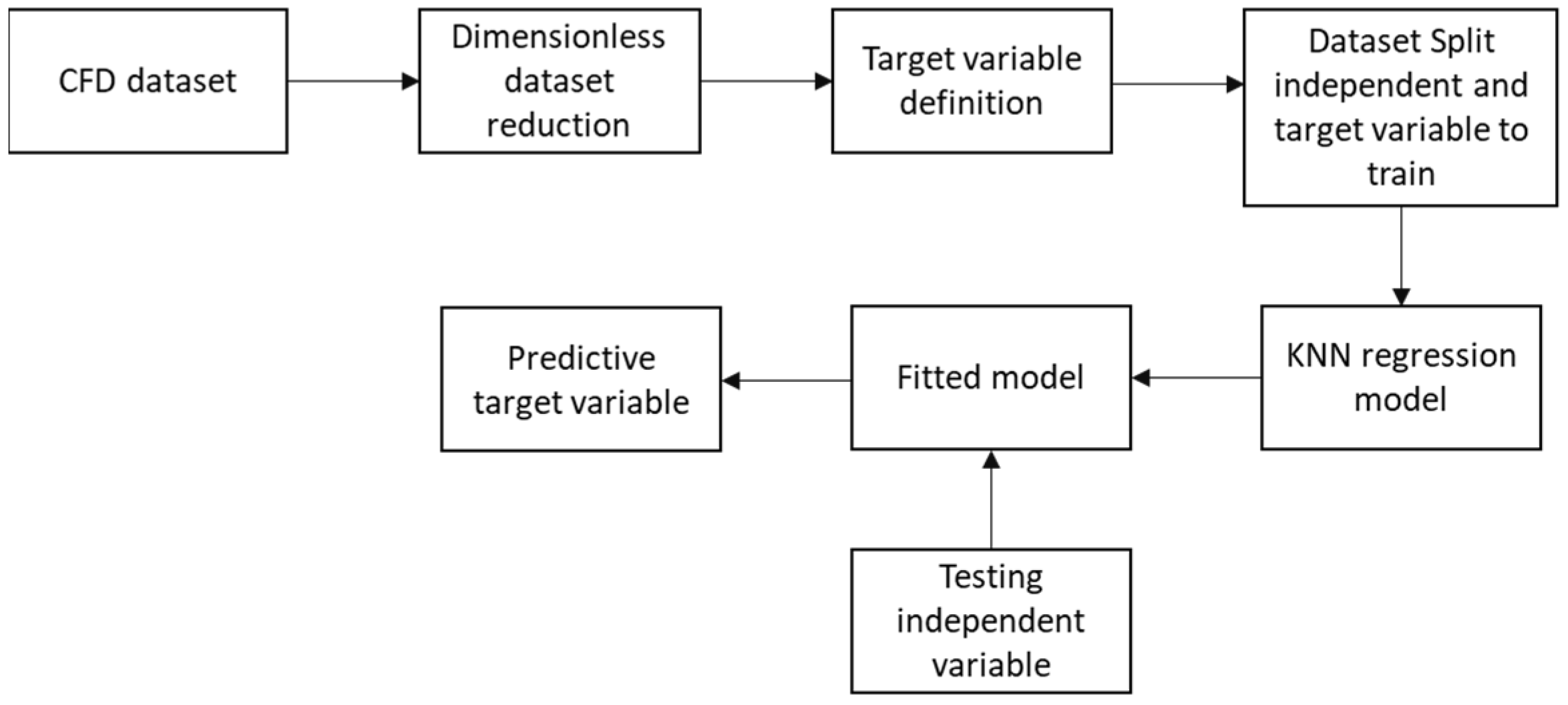
Considering the information previously mentioned, k-NN as regression has been selected as a method to predict drag performance (Figure 4).

The k-NN is calibrated by two parameters, “k” and “distance metric”, where “k” represents the number of neighbors considered and the “distance metric” measures the similarity between data points. By considering the k nearest neighbors and using a distance metric to measure similarity, the k-NN algorithm in regression can make predictions for new data points based on the patterns observed in the training data. The Euclidian distance is calculated as:

$${\mathit{d}}_{\mathit{i}\mathit{j}}=\sqrt{{\left({\mathit{x}}_{\mathit{i}}-{\mathit{x}}_{\mathit{j}}\right)}^{\mathbf{2}}+{\left({\mathit{z}}_{\mathit{i}}-{\mathit{z}}_{\mathit{j}}\right)}^{\mathbf{2}}}$$

(3)

The accuracy of predicted values is compared with simulation results using determination coefficient (R²) values, and the selection of “k” neighbors is based on model accuracy:

$${\mathit{R}}^{\mathbf{2}}=\mathbf{1}-{\displaystyle \frac{{\sum }_{\mathit{i}}{\left({\mathit{y}}_{\mathit{i}}-{\mathit{p}}_{\mathit{i}}\right)}^{\mathbf{2}}}{{\sum }_{\mathit{i}}{\left({\mathit{y}}_{\mathit{i}}-\overline{\mathit{y}}\right)}^{\mathbf{2}}}}$$

(4)

For experiments, 70% of the dataset is considered for training, while 30% is used for testing. Several k close neighbors are used, and prediction is computed based on Euclidean distance.

3. Results and Discussion

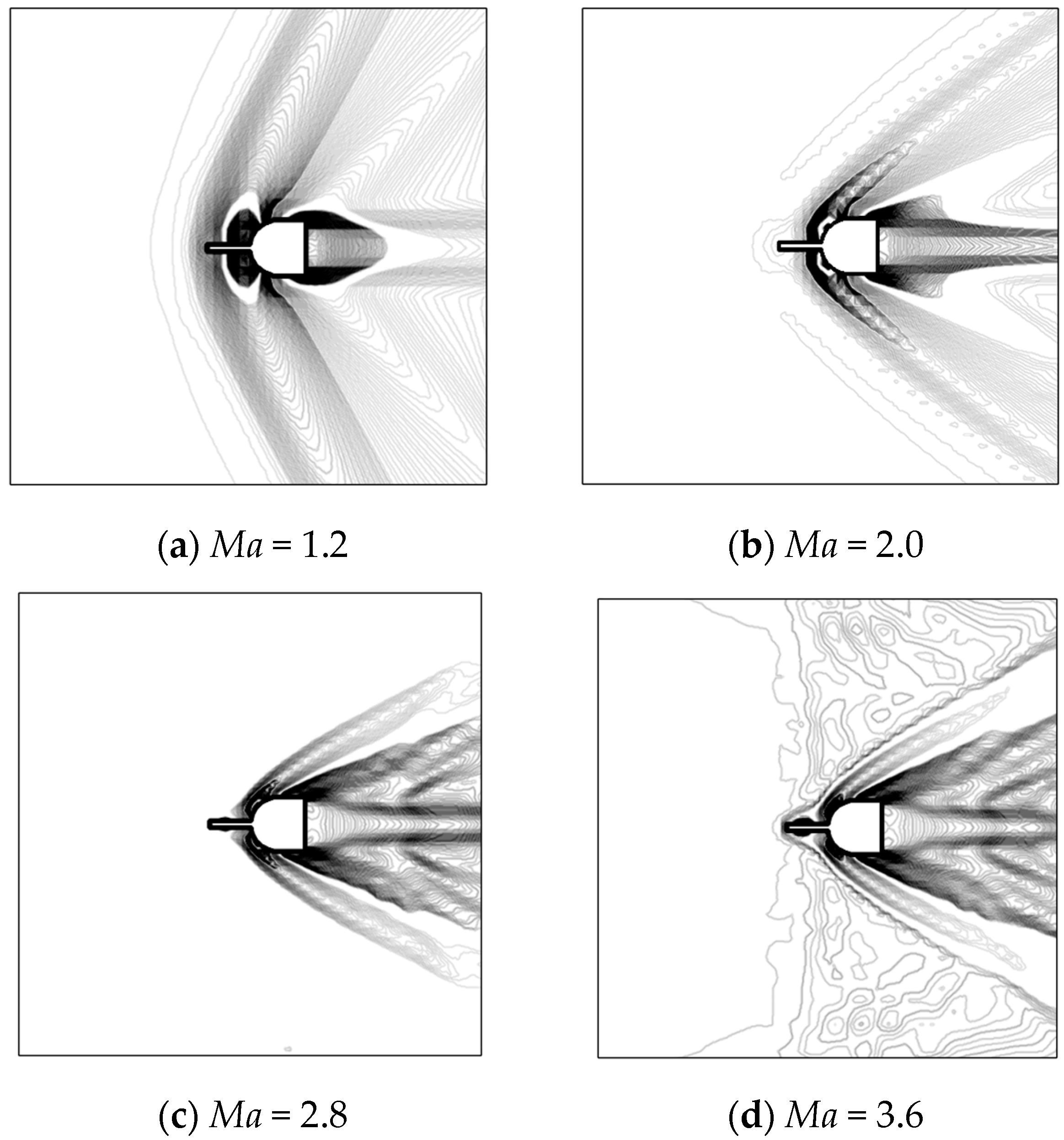
To show simulation performance and verify that simulations are capturing the phenomenon, Figure 5 presents the shock wave formation system by using the numerical Schlieren technique for four different Mach (Ma) numbers with the same geometrical relationship. This is conducted by visualizing the contours of the absolute density gradient (|∇ρ|) [37]. The images presented expose the overall flow behavior, demonstrating how the strong oblique shock wave found in blunt bodies is broken down into a group of lower-intensity shock waves. In Figure 5b–d, the characteristic recirculation and reattachment zones are observed, along with the reattachment shock wave seen in spiked blunt bodies under high Mach conditions [38]. However, for the Ma = 1.2, it is possible to see that the bow shock wave is only moved upstream in front of the spike, which is the reason why a significant reduction in drag is not achieved under transonic flow conditions. Therefore, the software is capable of adequately reproducing most of the physics involved in spike blunt bodies subjected to transonic and supersonic flow conditions. Thus, the capture of these flow characteristics makes a well-suited drag prediction by using the CFD Tool. Despite the fact that an axisymmetric can be performed to save time and useful cells, time simulation for the configuration selected takes around 10 min, time small enough to consider all body dimensions.

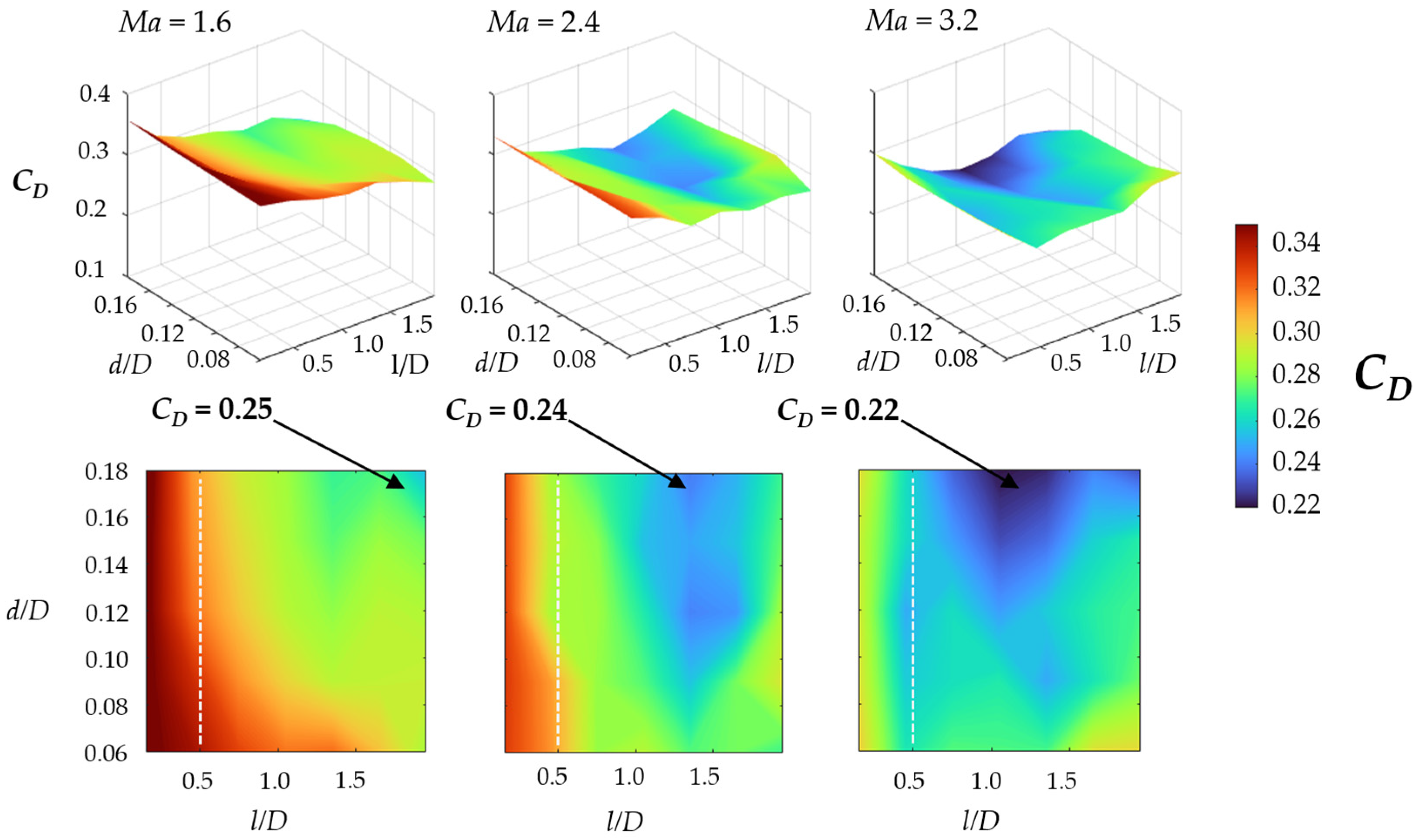
On the other hand, to show the effectiveness of the spike on the blunt body and the quality and relevance of the dataset used by the k-NN model, numerical simulation results of the drag coefficient are presented. The effectiveness of the spike is reflected in the aerodynamic drag reduction. Surface plots of C_D are shown in the upper part of Figure 6.

The surfaces in the upper part of Figure 6 might seem like each other, regardless of the aspect ratio of the spike (d/D or l/D), but the surfaces show lower values as the Ma increases. A first increase in the Ma (1.6→2.4) reduces the average drag coefficient (C_D,average) by 5.1%, and a second increase (2.4→3.2) reduces the coefficient by another 7.5%, as shown in

Table 3. Aerodynamics drag coefficient at different Ma.

Ma	CD,average	CD,min	CD,max
1.6	0.306	0.253	0.358
2.4	0.282	0.240	0.332
3.2	0.263	0.221	0.299

.

As shown in the lower part of Figure 6, the general tendency of the C_D is to reduce its value as the spike length increases, which is consistent with several works [10,11,12,13,14,15,16]. Within our range of spike length ratio values above one time, the blunt body diameter presents the best performance. For short spike length ratios (lower than 0.5), this extruded geometry from the blunt body is ineffective in reducing the drag force. The primary shock wave formed by the spike does not affect the secondary shock wave of the blunt body, and it occurs at any spike diameter ratio.

Until this point, this study has provided insights that explain drag coefficient performance for a flat spike blunt body with respect to Mach number, Reynolds number, dimensionless spike diameter ratio, and dimensionless spike length ratio. As mentioned in previous sections, to identify that the phenomenon was captured correctly, the numerical Schlieren technique is used to identify shockwave formations and drag reduction; Figure 5. All simulations were performed on the same computer (Dell Precision 7530 wkst intel core Xeon e-2176m/memory 16 GB). On average, simulation takes 10 min per case. The Python sklearn library is used to implement the k-NN model. To train it, 70% of the total dataset was used for training, while 30% for testing. The k-NN model was tested for different neighbors to identify proper numbers.

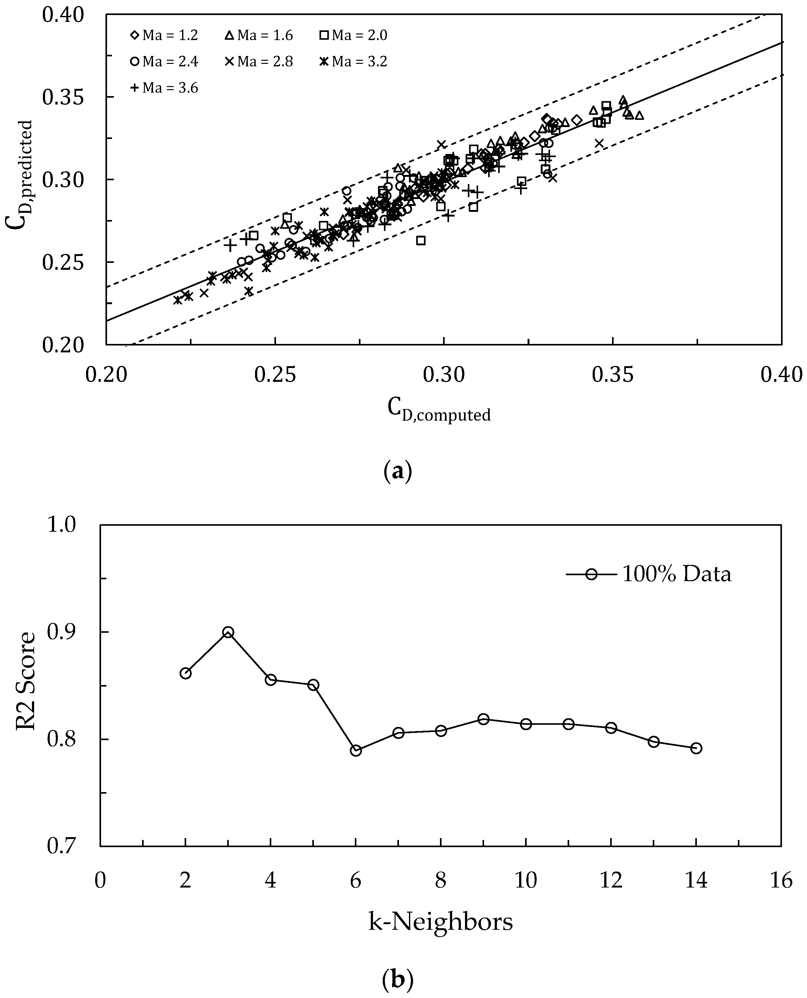
Figure 7 presents the results of the k-NN model and test error for different neighbors’ numbers. Figure 7a shows a comparison of tested data against model-predicted values. It can be observed that for drag coefficient prediction, 209 out of 239 data points lie within the ±5% error range, around 87% of total data, which is consistent with previous studies that combined computational fluid dynamics and the k-NN model [39].

Different k neighbors were tested and recorded. Figure 7b shows that k = 3 predicts the highest accuracy for drag reduction; the R² value for drag reduction is 0.90. The k-NN regression algorithm demonstrates impressive accuracy, making it an excellent tool for engineers to predict outputs without the need for computationally solving the drag reduction system.

Figure 8 shows the error difference between $C_D$ computed and $C_D$ predicted for 100% of the data simulation and a random sample of 70% of the dataset. In this case, it is possible to observe that despite accuracy decreases for 70% of the sample, there is still a significant amount of data lying in 10% error.

$$\%Error={\displaystyle \frac{ABS\left[C_{D,Computed}-C_{D,Predicted}\right]}{C_{D,Computed}}}$$

(5)

Due time is critical for CFD practitioners, and dataset creation can be substantially time-consuming. A set of similar tests was performed, reducing the amount of data by 70% and 50% and generating aleatory dataset samples, respectively, to test the average amount of data predicted lying with ±10% error.

Table 4. Aleatory sample accuracy.

Sample Size	# of Points < 10% Error	% Accuracy
168	150	89%
120	103	85%

presents average errors considering different samples.

According to Table 4, datasets with 70% of the total dataset present that, on average, 89% of data lying in error under 10%, while datasets with 50% of the total dataset did it at approximately 85%. This result presents similar performances to the work presented by Krishnayatra [40], where almost the same amount of data presents similar results.

In computational fluid dynamics, metamodels have been used as a popular tool to respond to expensive simulations. The Kriging method has been used previously to generate a high-fidelity model in the context of the drag performance of a spike blunt body [39]. Kriging is a geostatistical interpolation method used to predict the values of a variable at unsampled points collected from the values of that variable at sampled points. To test k-NN accuracy, ordinary Kriging was used throughout the scikit-learn Python library. Ordinary Kriging is a balanced and robust option that works properly in a wide variety of situations, especially when there are no clear spatial trends or detailed knowledge of the global mean of the process. It is the preferred choice when looking for reliable interpolation without making strong assumptions about the underlying structure of the data.

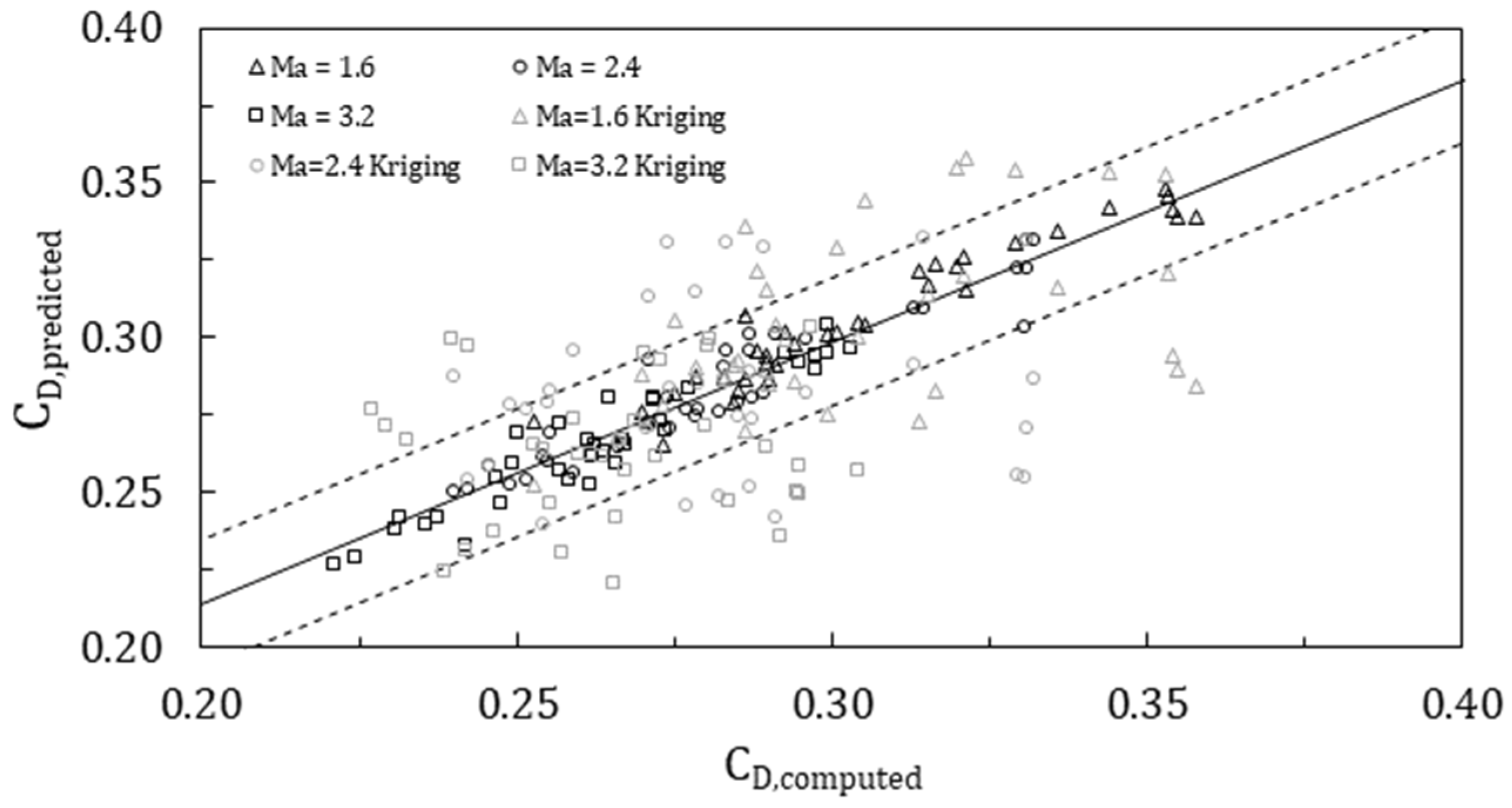
Figure 9 shows the prediction provided by the k-NN model and Kriging prediction for Ma = 1.6, 2.4, and 3.2. Here, it is possible to observe that predictions provided by the k-NN model present accuracy close to 95%, while many Kriging predictions fall out of this range. Besides significantly better performance, k-NN provides a prediction for all ranges of geometrical and flow conditions characteristics considered. Kriging model prediction must be built keeping constant flow conditions, modifying geometrical characteristics. In this sense, k-NN must be trained just once, testing the best number of neighbors, while Kriging implementation must be repeated for each flow condition considered. If Kriging’s performance must be improved, more simulations must be conducted, which implies an increase in dataset size. k-NN can provide proper results even with 70% of the dataset considered for this study.

4. Conclusions

This study provides insights into the physical variations in the overall drag coefficient reduction in a flat spike blunt with respect to force over x direction, velocity, density, viscosity, speed of sound, spike diameter, and spike length. Parameters were reduced to their non-dimensional form. Therefore, Mach number Ma variates from 1.2 to 3.6, d/D dimensionless spike diameter ratio and l/D spike length ratio ranged from 0.06 to 0.18 and from 0.15 to 2.15 times blunt body diameter, respectively.

According to the results presented in this research, Solidworks flow simulation with selected mesh has been able to capture shock wave performance. We observe the recirculation and reattachment zone at supersonic flow conditions Ma = 2.0, 2.8, and 3.6. For Ma = 1.2, the bow shock wave is only moved upstream in front of the spike, which is the reason why a significant reduction in drag is not achieved. On the other hand, it is observed that as soon as the Ma number increases, the drag coefficient reduces between 5% and 7.5%.

Despite machine learning emerging as a valuable tool, its implementation can be privative when there is a lack of computational sources or expertise in machine learning. In this sense, k-NN has shown that it can be a suitable model, not just for the accuracy or its easy implementation; the use of a small dataset makes it appropriate to create in a small time period enough data to predict performance. According to the methodology used, the reduction in data through dimensionless parameters in conjunction with the k-NN model has presented an accuracy close to 95%, and even by reducing the dataset, good performance can be obtained. k-NN was tested again by the Kriging method, showing significantly better performance. While Kriging implementation must be repeated for each flow condition, keeping constant geometrical conditions, k-NN can predict for all ranges of geometrical and flow conditions considered.

Future research will focus on applying the current methodology for parameters such as heat transfer as well as other physical characteristics like angle attack or changes over spike geometrical shapes.

References

1. Anderson, J.D. Fundamentals of Aerodynamics, 6th ed.; McGraw-Hill: New York, NY, USA, 2017. [Google Scholar]
2. Rashid, S.; Nawaz, F.; Maqsood, A.; Salamat, S.; Riaz, R. Review of Wave Drag Reduction Techniques: Advances in Active, Passive, and Hybrid Flow Control. Proc. Inst. Mech. Eng. G J. Aerosp. Eng. 2022, 236, 2851–2884. [Google Scholar] [CrossRef]
3. Bertin, J.J.; Cummings, R.M. Fifty Yxears of Hypersonics: Where We’ve Been, Where We’re Going. Prog. Aerosp. Sci. 2003, 39, 511–536. [Google Scholar] [CrossRef]
4. Bertin, J.J.; Bouslog, S.A.; Wang, K.-C.; Campbell, C.H. Recent Aerothermodynamic Flight Measurements during Shuttle Orbiter Re-Entry. J. Spacecr. Rocket. 1996, 33, 457–462. [Google Scholar] [CrossRef]
5. Schneider, S.P. Flight Data for Boundary-Layer Transition at Hypersonic and Supersonic Speeds. J. Spacecr. Rocket. 1999, 36, 8–20. [Google Scholar] [CrossRef]
6. Hollis, B.R.; Borrelli, S. Aerothermodynamics of Blunt Body Entry Vehicles. Prog. Aerosp. Sci. 2012, 48–49, 42–56. [Google Scholar] [CrossRef]
7. Huang, W.; Chen, Z.; Yan, L.; Yan, B.; Du, Z. Drag and Heat Flux Reduction Mechanism Induced by the Spike and Its Combinations in Supersonic Flows: A Review. Prog. Aerosp. Sci. 2019, 105, 31–39. [Google Scholar] [CrossRef]
8. Guenther, R.A.; Reding, J.P. Fluctuating Pressure Environment of a Drag Reduction Spike. J. Spacecr. Rocket. 1977, 14, 705–710. [Google Scholar] [CrossRef]
9. Ahmed, M.Y.M.; Qin, N. Recent Advances in the Aerothermodynamics of Spiked Hypersonic Vehicles. Prog. Aerosp. Sci. 2011, 47, 425–449. [Google Scholar] [CrossRef]
10. Esfeh, M.K.; Tajalli, S.M.; Liu, P. Evaluation of Aerospike for Drag Reduction on a Blunt Nose Using Experimental and Numerical Modeling. Acta Astronaut. 2019, 160, 656–671. [Google Scholar] [CrossRef]
11. Tekure, V.; Pophali, P.S.; Venkatasubbaiah, K. Numerical Investigation of Aerospike Semi-Cone Angle and a Small Bump on the Spike Stem in Reducing the Aerodynamic Drag and Heating of Spiked Blunt-Body: New Correlations for Drag and Surface Temperature. Phys. Fluids 2021, 33, 116108. [Google Scholar] [CrossRef]
12. Kalimuthu, R.; Mehta, R.C.; Rathakrishnan, E. Investigation of Aerodynamic Coefficients at Mach 6 over Conical, Hemispherical and Flat-Face Spiked Body. Aeronaut. J. 2017, 121, 1711–1732. [Google Scholar] [CrossRef]
13. Li, Z.; Sun, C.; Xia, X.; Li, X. Numerical Simulation of Aerodynamic Heating over Solid Blunt Configuration with Porous Spike. J. Aerosp. Eng. 2018, 31, 04018083. [Google Scholar] [CrossRef]
14. Asif, M.; Zahir, S.; Kamran, N.; Khan, M. Computational Investigations Aerodynamic Forces at Supersonic/Hypersonic Flow Past a Blunt Body with Various Forward Facing Spikes. In Proceedings of the 22nd Applied Aerodynamics Conference and Exhibit, Guidance, Navigation, and Control and Co-located Conferences, AIAA, Providence, RI, USA, 16–19 August 2004. [Google Scholar]
15. Xue, Y.; Wang, L.; Fu, S. Drag Reduction and Aerodynamic Shape Optimization for Spike-Tipped Supersonic Blunt Nose. J. Spacecr. Rocket. 2018, 55, 552–560. [Google Scholar] [CrossRef]
16. Hamza, M.; Khan, S.B.; Maqsood, A. Geometric Optimization of Blunt Bodies with Aerodisk and Opposing Jet for Wave Drag and Heat Reduction. Aerospace 2022, 9, 800. [Google Scholar] [CrossRef]
17. Brunton, S.L.; Noack, B.R.; Koumoutsakos, P. Machine Learning for Fluid Mechanics. Annu. Rev. Fluid Mech. 2020, 52, 477–508. [Google Scholar] [CrossRef]
18. Vinuesa, R.; Brunton, S.L. Enhancing Computational Fluid Dynamics with Machine Learning. Nat. Comput. Sci. 2022, 2, 358–366. [Google Scholar] [CrossRef]
19. Kou, J.; Zhang, W. Data-Driven Modeling for Unsteady Aerodynamics and Aeroelasticity. Prog. Aerosp. Sci. 2021, 125, 100725. [Google Scholar] [CrossRef]
20. Li, J.; Du, X.; Martins, J.R.R.A. Machine Learning in Aerodynamic Shape Optimization. Prog. Aerosp. Sci. 2022, 134, 100849. [Google Scholar] [CrossRef]
21. Bianco, M.J.; Gerstoft, P.; Traer, J.; Ozanich, E.; Roch, M.A.; Gannot, S.; Deledalle, C.-A. Machine Learning in Acoustics: Theory and Applications. J. Acoust. Soc. Am. 2019, 146, 3590–3628. [Google Scholar] [CrossRef]
22. Kužnar, D.; Možina, M.; Giordanino, M.; Bratko, I. Improving Vehicle Aeroacoustics Using Machine Learning. Eng. Appl. Artif. Intell. 2012, 25, 1053–1061. [Google Scholar] [CrossRef]
23. Alguacil, A.; Bauerheim, M.; Jacob, M.C.; Moreau, S. Predicting the Propagation of Acoustic Waves Using Deep Convolutional Neural Networks. J. Sound Vib. 2021, 512, 116285. [Google Scholar] [CrossRef]
24. Salehi, H.; Das, S.; Chakrabartty, S.; Biswas, S.; Burgueño, R. Damage Identification in Aircraft Structures with Self-Powered Sensing Technology: A Machine Learning Approach. Struct. Control Health Monit. 2018, 25, e2262. [Google Scholar] [CrossRef]
25. de Jong, M.; Chen, W.; Notestine, R.; Persson, K.; Ceder, G.; Jain, A.; Asta, M.; Gamst, A. A Statistical Learning Framework for Materials Science: Application to Elastic Moduli of k-Nary Inorganic Polycrystalline Compounds. Sci. Rep. 2016, 6, 34256. [Google Scholar] [CrossRef] [PubMed]
26. Linse, D.J.; Stengel, R.F. Identification of Aerodynamic Coefficients Using Computational Neural Networks. J. Guid. Control Dyn. 1993, 16, 1018–1025. [Google Scholar] [CrossRef]
27. Suresh, S.; Omkar, S.N.; Mani, V.; Guru Prakash, T.N. Lift Coefficient Prediction at High Angle of Attack Using Recurrent Neural Network. Aerosp. Sci. Technol. 2003, 7, 595–602. [Google Scholar] [CrossRef]
28. Secco, N.R.; De Mattos, B.S. Artificial Neural Networks to Predict Aerodynamic Coefficients of Transport Airplanes. Aircr. Eng. Aerosp. Technol. 2017, 89, 211–230. [Google Scholar] [CrossRef]
29. Ghoreyshi, M.; Jirásek, A.; Cummings, R.M. Computational Approximation of Nonlinear Unsteady Aerodynamics Using an Aerodynamic Model Hierarchy. Aerosp. Sci. Technol. 2013, 28, 133–144. [Google Scholar] [CrossRef]
30. Wang, X.; Kou, J.; Zhang, W. Unsteady Aerodynamic Modeling Based on Fuzzy Scalar Radial Basis Function Neural Networks. Proc. Inst. Mech. Eng. G J. Aerosp. Eng. 2019, 233, 5107–5121. [Google Scholar] [CrossRef]
31. Hou, W.; Darakananda, D.; Eldredge, J.D. Machine-Learning-Based Detection of Aerodynamic Disturbances Using Surface Pressure Measurements. AIAA J. 2019, 57, 5079–5093. [Google Scholar] [CrossRef]
32. Taunk, K.; De, S.; Verma, S.; Swetapadma, A. A Brief Review of Nearest Neighbor Algorithm for Learning and Classification. In Proceedings of the 2019 International Conference on Intelligent Computing and Control Systems (ICCS), Madurai, India, 15–17 May 2019; pp. 1255–1260. [Google Scholar]
33. Numerical Basis of CAD-Embedded CFD: White Paper. Available online: https://www.solidworks.com/sw/docs/Flow_Basis_of_CAD_Embedded_CFD_Whitepaper.pdf (accessed on 1 June 2024).
34. Ingram, D.M.; Causon, D.M.; Mingham, C.G. Developments in Cartesian Cut Cell Methods. Math. Comput. Simul. 2003, 61, 561–572. [Google Scholar] [CrossRef]
35. Hodges, A.J. The Drag Coefficient of Very High Velocity Spheres. J. Aeronaut. Sci. 1957, 24, 755–758. [Google Scholar] [CrossRef]
36. Charters, A.C.; Thomas, R.N. The Aerodynamic Performance of Small Spheres from Subsonic to High Supersonic Velocities. J. Aeronaut. Sci. 1945, 12, 468–476. [Google Scholar] [CrossRef]
37. Ahmad, H.; Hasan, N.; Sanghi, S. On the Influence of Co-Flow on the Shocks and Vortex Rings in the Starting Phases of under-Expanded Jets. Phys. Fluids 2022, 34, 076117. [Google Scholar] [CrossRef]
38. Tahani, M.; Karimi, M.S.; Motlagh, A.M.; Mirmahdian, S. Numerical Investigation of Drag and Heat Reduction in Hypersonic Spiked Blunt Bodies. Heat Mass Transf. 2013, 49, 1369–1384. [Google Scholar] [CrossRef]
39. Ahmed, M.Y.M.; Qin, N. Metamodels for aerothermodynamic design optimization of hypersonic spiked blunt bodies. Aerosp. Sci. Technol. 2010, 14, 364–376. [Google Scholar] [CrossRef]
40. Krishnayatra, G.; Tokas, S.; Kumar, R. Numerical Heat Transfer Analysis & Predicting Thermal Performance of Fins for a Novel Heat Exchanger Using Machine Learning. Case Stud. Therm. Eng. 2020, 21, 100706. [Google Scholar] [CrossRef]
Figure 1. Mach number versus aerodynamics drag coefficient.
Aerospace 11 00757 g001
Figure 2. Blunt body scheme with main dimensions.
Aerospace 11 00757 g002
Figure 3. Computational domain dimension. The domain is embodied in a structured mesh with an irregular grid close to the spike blunt body.
Aerospace 11 00757 g003
Figure 4. k-NN and CFD implementation.
Aerospace 11 00757 g004
Figure 5. Shock wave formation: Numerical Schlieren for four different Mach numbers with the same geometrical relationship (l/D = 1.05 and d/D = 0.12). The strong oblique shock wave found in blunt bodies is broken down into a series of lower-intensity shock waves.
Aerospace 11 00757 g005
Figure 6. Drag coefficient surfaces and contours at different. The CD surfaces move to lower levels as the Ma increases. On average, the lowest coefficients have a general tendency; they are obtained for spike diameter around 0.17 times the blunt body diameter and spike length 1.4 times the blunt body diameter.
Aerospace 11 00757 g006
Figure 7. (a) Computed drag coefficient vs. predicted drag coefficient and (b) k-neighbors vs. determination coefficient.
Aerospace 11 00757 g007
Figure 8. Error percentage per predicted point.
Aerospace 11 00757 g008
Figure 9. Comparison of k-NN prediction vs. Kriging prediction (dashed lines represent prediction limits with errors under 5%).
Aerospace 11 00757 g009