Article

Autonomous Trajectory Planning Method for Stratospheric Airship Regional Station-Keeping Based on Deep Reinforcement Learning

1
Aerospace Information Research Institute, Chinese Academy of Sciences, Beijing 100094, China
2
University of Chinese Academy of Sciences, Beijing 100190, China
*
Authors to whom correspondence should be addressed.
Aerospace 2024, 11(9), 753; https://doi.org/10.3390/aerospace11090753
Submission received: 6 August 2024 / Revised: 2 September 2024 / Accepted: 11 September 2024 / Published: 13 September 2024
(This article belongs to the Section Astronautics & Space Science)

Abstract

:
The stratospheric airship, as a near-space vehicle, is increasingly utilized in scientific exploration and Earth observation due to its long endurance and regional observation capabilities. However, due to the complex characteristics of the stratospheric wind field environment, trajectory planning for stratospheric airships is a significant challenge. Unlike lower atmospheric levels, the stratosphere presents a wind field characterized by significant variability in wind speed and direction, which can drastically affect the stability of the airship’s trajectory. Recent advances in deep reinforcement learning (DRL) have presented promising avenues for trajectory planning. DRL algorithms have demonstrated the ability to learn complex control strategies autonomously by interacting with the environment. In particular, the proximal policy optimization (PPO) algorithm has shown effectiveness in continuous control tasks and is well suited to the non-linear, high-dimensional problem of trajectory planning in dynamic environments. This paper proposes a trajectory planning method for stratospheric airships based on the PPO algorithm. The primary contributions of this paper include establishing a continuous action space model for stratospheric airship motion; enabling more precise control and adjustments across a broader range of actions; integrating time-varying wind field data into the reinforcement learning environment; enhancing the policy network’s adaptability and generalization to various environmental conditions; and enabling the algorithm to automatically adjust and optimize flight paths in real time using wind speed information, reducing the need for human intervention. Experimental results show that, within its wind resistance capability, the airship can achieve long-duration regional station-keeping, with a maximum station-keeping time ratio (STR) of up to 0.997.

1. Introduction

In recent years, with the development of aerospace technology, near-space vehicles have become the focus of research in various countries [1]. Near space refers to the area of the atmosphere between 20 km and 100 km above the Earth’s surface. Conventional aircraft struggle to reach this altitude range, and satellites cannot maintain a stable orbit at this altitude [2]. The stratospheric airship, as a type of near-space vehicle, has advantages such as long flight duration and large payload capacity. It can perform long-duration missions at altitudes of 18 km to 22 km [3], making it an ideal platform for tasks like navigation, environmental monitoring, and scientific experiments [4].
The stratospheric airship mainly relies on buoyancy to maintain flight altitude. To achieve greater carrying capacity, airships typically require a large capsule to store helium, resulting in a large windward area and high drag coefficient. Consequently, the stratospheric airship is significantly affected by wind during flight [5,6]. The stratospheric wind field is characterized by its complexity and unpredictability, with wind speeds varying significantly with altitude and latitude. This complex wind environment presents enormous challenges for trajectory planning, especially for regional station-keeping missions in specific areas. The wind resistance capability of the stratospheric airship is on the same order of magnitude as the stratospheric wind field. Therefore, to achieve better trajectory planning, the impact of the wind field must be taken into account. When the wind speed exceeds the airship’s maximum airspeed, the airship will drift out of the designated mission area [7]. Additionally, strategies for the airship to return to the mission area after the wind subsides must also be considered [8].
Trajectory planning is a critical issue in the fields of Robotics, Autonomous Vehicles, and Uncrewed Aerial Vehicles (UAVs). Traditional methods include graph search algorithms, sampling methods, and optimization algorithms. Graph search algorithms, such as the A* algorithm [9] and Dijkstra algorithm [10], are effective for model construction but often suffer from low path-search efficiency and cannot guarantee optimal paths. Sampling algorithms, including the Rapidly exploring Random Tree (RRT) [11] and Probabilistic Road Map (PRM) [12], can find optimal paths but converge slowly. Intelligent optimization algorithms, such as Ant Colony Optimization (ACO) [13], Genetic Algorithm (GA) [14], and Simulated Annealing (SA) [15], are simple to implement but can become stuck in local optima or fail to reach the target. For stratospheric airship trajectory planning, due to the dynamic characteristics of stratospheric wind field, the traditional trajectory planning method is difficult to adjust the airship course in real time, and usually cannot take into account the time variability and unpredictability of stratospheric wind field, leading to suboptimal planning results. In contrast, trajectory planning methods based on deep reinforcement learning (DRL) offer greater adaptability and robustness by continuously learning and optimizing the airship’s flight strategy in response to real-time wind conditions.
In recent years, the development of deep reinforcement learning (DRL) has presented new opportunities for trajectory planning [16,17]. Combining the perception capability of deep learning and the decision-making ability of reinforcement learning, DRL enables agents to autonomously learn trajectory planning strategies in complex environments through constant trial and error [18]. At present, although research on trajectory planning based on DRL is relatively limited in the field of stratospheric airships, it has been widely applied in the fields of Robotics [19,20], Autonomous Ships [21,22], UAVs [23,24], and Avs [25,26], providing important reference value for the trajectory planning of stratospheric airships. Lei et al. [27] used the Double Deep Q-Network (DDQN) algorithm for the dynamic trajectory planning of mobile robots in unknown environments. Xie et al. [28] implemented a 3D path planning method for UAVs in large-scale dynamic environments using an improved Deep Recurrent Q-Network (DRQN) algorithm. Ni et al. [29] proposed a method based on Soft Actor–Critic to optimize the trajectory of High-Altitude Long-Endurance (HALE) solar-powered aircraft, which can improve battery energy utilization and flight duration compared to other strategies. Zhu et al. [30] proposed a dynamic obstacle avoidance method for Autonomous Underwater Vehicles (AUVs) based on an improved proximal policy optimization (PPO) algorithm. Josef et al. [31] adopted an improved Rainbow algorithm for the safe local trajectory planning of ground vehicles in unknown rugged terrain. Zheng et al. [32] proposed a discrete action space path planning method for stratospheric airships based on the DRQN algorithm, enabling autonomous decision making in dynamic wind fields. Yang et al. [33] proposed an adaptive horizontal trajectory control method for stratospheric airships based on the Q-learning algorithm. This method decomposes horizontal trajectory control into target tracking and constructs an observation model for the airships. Nie et al. [34] developed a model-free control strategy for stratospheric airships using reinforcement learning. They proposed an adaptive method for discretizing the state space and established a Markov Decision Process (MDP) model to guide the control strategy. However, the path planning method for discrete action spaces may be limited in some cases because it cannot accurately capture the complex motion of the airship in a continuous space. The above DRL-based trajectory planning methods have proved their effectiveness and practical value in trajectory planning tasks. However, DRL methods still face some challenges, such as high sample complexity and poor convergence, requiring careful adjustment of neural network parameters.
In this study, we propose an autonomous trajectory planning method for stratospheric airships based on the PPO algorithm for regional station-keeping. By designing state space, action space, and reward functions, we train the flight strategy of the airship and test the trained model under different wind field conditions. The main contributions of this paper are as follows:
  • This paper proposes a DRL-based continuous action space 2D trajectory planning method. Compared to methods with discrete action spaces, this method provides the airship with higher flexibility and smoother flight trajectories. During flight, the airship can make reasonable flight decisions by considering the wind field environment and its own state, allowing it to reach the target area and achieve long-duration station-keeping.
  • Our approach is based on a time-varying wind field that reflects the dynamic characteristics of wind speed and direction changes over time. The action of the airship does not depend on past or future wind field states but is based on current real-time wind speed information. By adjusting and optimizing the flight path in real-time, the airship can automatically navigate and reduce the need for human intervention.
The structure of this paper is as follows: Section 2 describes the airship’s kinematic model and the stratospheric wind field environment. Section 3 introduces the PPO algorithm and sets up the observation space, action space, and reward function. Section 4 presents and discusses the training and testing results of the model. Section 5 concludes this paper and envisages future work.

2. Problem Formulation

In this section, the kinematic airship model and the complex stratospheric wind environment are described.

2.1. The Kinematic Airship Model

In order to simplify the kinematic model, the following assumptions are made in this paper:
  • The airship has large inertia and weak wind resistance, making it significantly susceptible to wind field effects.
  • The airship is simplified as a particle.
  • The airship usually does not have the ability to actively adjust its height and does not consider the vertical movement of the airship, only considering the movement of the fixed isobaric surface.
  • Only the kinematic characteristics of the airship are considered.
  • The wind field is assumed to be constant within a ∆t time interval, and the airship’s displacement due to the wind is equal to the wind displacement during the ∆t time interval.
The ground speed of the airship in a horizontal wind field can be obtained from the vector sum of its airspeed and wind speed. Therefore, in order to simplify the derivation process, the displacement of the airship is also divided into two parts: one caused by its airspeed, which is the displacement generated by its own driving force, and the other caused by the influence of the wind field, as shown in Figure 1.
In Figure 1, v a , v w , and v g represent the airspeed, wind speed, and ground speed of the airship at time t , ( x g , y g ) are the airship’s position at time t , and θ is the heading of the airship at time t . v a , v w , and v g represent the airspeed, wind speed, and ground speed of the airship at time t + t , ( x g , y g ) are the airship’s position at time t + t , and θ is the heading of the airship at time t + t . u and v are the components of the wind speed in the x and y directions. Thus, the displacement of the airship in the x and y directions in the time interval t can be expressed as
x g = x a + x w y g = y a + y w
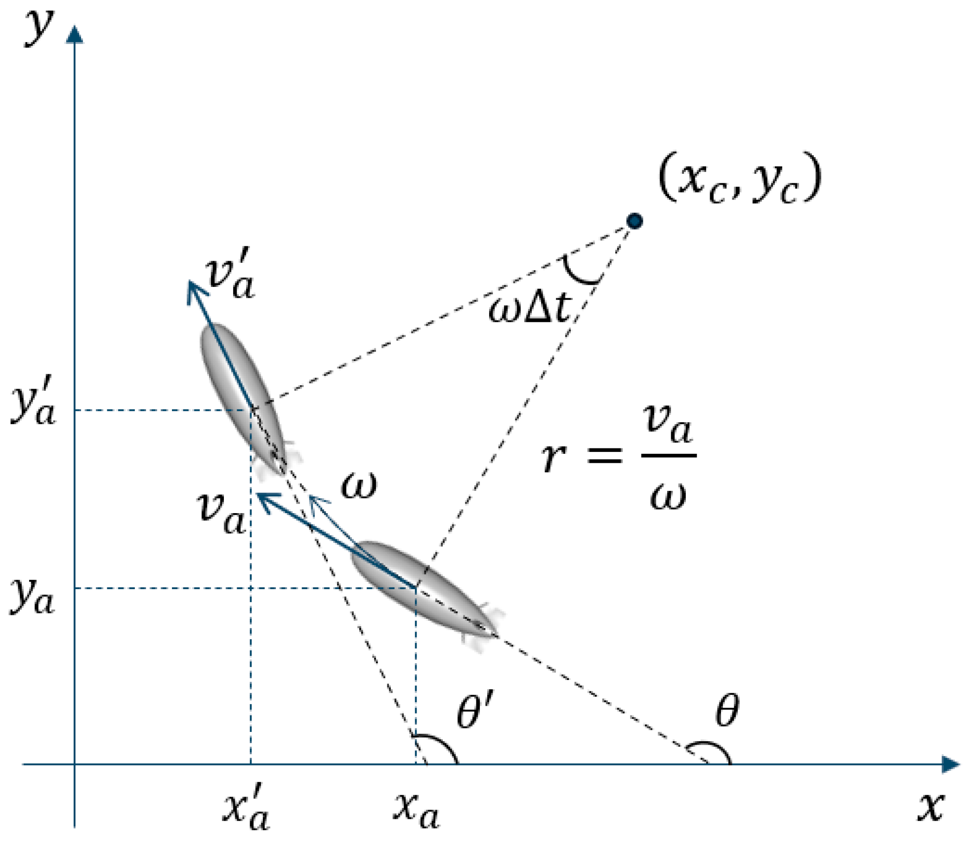
Regardless of the wind speed, the movement of the airship can be regarded as an arc in a small time interval. The motion process of the airship can be described by two parameters: the airspeed v a and the angular velocity ω , as shown in Figure 2. ( x c , y c ) is the center of the arc, and r is the turning radius. From the geometric relationship, the center of the arc can be deduced as follows:
      x c = x a v a ω sin θ     y c = y a + v a ω cos θ
The position of the airship at time t + t can be calculated as
      x a = x c + v a ω sin ( θ + ω t ) = x a v a ω sin θ + v a ω sin ( θ + ω t ) y a = y c + v a ω cos ( θ + ω t ) = y a + v a ω cos θ + v a ω cos ( θ + ω t )
Therefore, the displacement of the airship itself can be deduced as follows:
      x a = x a x a = v a ω sin θ + v a ω sin ( θ + ω t ) y a = y a y a = v a ω cos θ + v a ω cos ( θ + ω t )
The displacement of the airship influenced by the wind within the t time interval can be defined as follows:
    x w = u t y w = v t
According to (1), (4), and (5), the kinematic model of the airship can be described as
x g y g θ = x g y g θ + v a ω ( sin θ + sin ( θ + ω t ) ) v a ω ( cos θ + cos ( θ + ω t ) ) ω t + u t v t 0

2.2. Description of Stratospheric Complex Wind Field Environment

The stratosphere is located approximately 10 km to 50 km above the Earth’s surface, where the wind field environment is highly complex, with significant variations in wind speed and direction across different latitudes, longitudes, altitudes, and times of the year. Due to the limited propulsion of the stratospheric airship, maintaining stable regional station-keeping in such a complex wind field environment becomes particularly challenging. To achieve effective regional station-keeping, the airship needs to adapt to the changes in the wind field and utilize the wind to control their position [35].
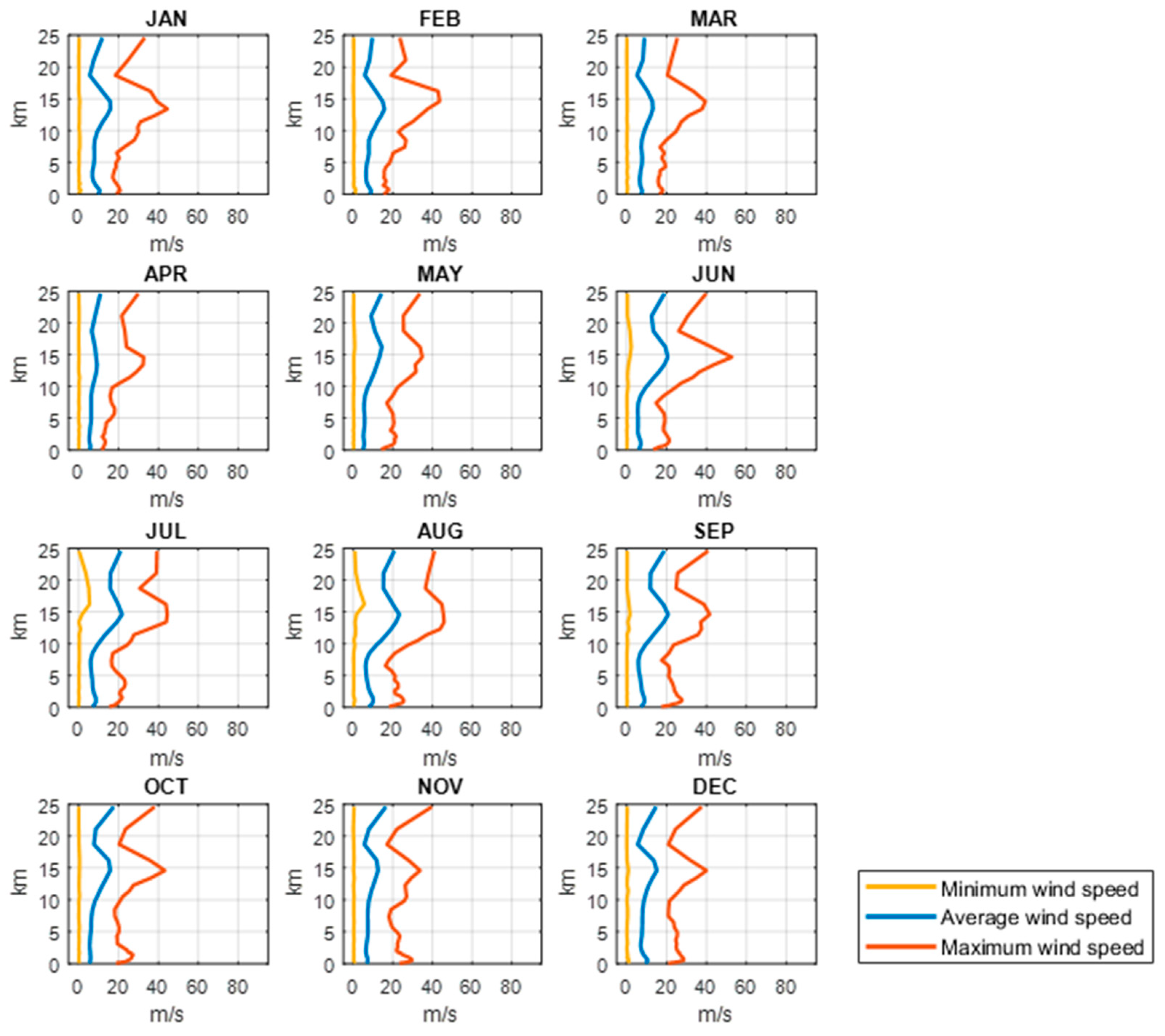
In this study, we selected ERA5 reanalysis data as the wind field data source [36]. Taking 10° N latitude as an example, we analyzed the ERA5 reanalysis wind field data from 2015 to 2024. The minimum, average, and maximum wind speeds from the surface to 25 km for different months are shown in Figure 3. It can be observed that a noticeable weak wind region exists at an altitude of 18 km to 22 km, which could provide an ideal regional station-keeping environment for stratospheric airships. In terms of magnitude, the maximum wind speed is around 20 m/s to 25 m/s, which aligns with the common wind resistance capability of airships. This has a significant impact on the trajectory planning of the airship.
ERA5 data have the characteristics of high temporal and spatial resolution, ensuring that the model can learn the finer features and changes in the wind field. Although the ERA5 data have a high resolution, it may not be sufficient to capture all the local variations in the wind field due to the inherent uncertainties in the stratosphere. However, compared to other datasets, the ERA5 reanalysis data offer comprehensive coverage and relatively higher accuracy, which is why we chose ERA5 as the training dataset. For the autonomous trajectory planning tasks of the stratospheric airship, high-resolution and high-accuracy data are crucial for simulating the dynamic changes in the wind field environment, which helps improve the model’s adaptability and generalization under different wind field environments. The ERA5 wind field data used in this study have a spatial resolution of 0.25° × 0.25°, a temporal resolution of 1 h, and a pressure level of 50 hPa (approximately 20 km in altitude).

3. DRL Model for Airship Trajectory Planning

In this section, we mainly introduce the proximal policy optimization algorithm and the design of the model’s network structure, state space, action space, and reward function.

3.1. Introduction to Proximal Policy Optimization

Proximal policy optimization (PPO) is a deep reinforcement learning algorithm proposed by OpenAI in 2017 [37]. The algorithm is based on the Actor–Critic architecture, where the Actor is responsible for taking actions given the current state, and the Critic is responsible for evaluating the value of those actions to guide the updates of the Actor network. This gradually enhances the agent’s decision-making ability in complex environments and is well suited for continuous control tasks. Compared to other popular algorithms such as Deep Deterministic Policy Gradient (DDPG) and Soft Actor–Critic (SAC), PPO offers several advantages that make it an ideal choice for airship trajectory planning in complex stratospheric environments. Unlike DDPG, which can be sensitive to hyperparameters and prone to instability during training, PPO employs a clipped objective function that prevents large updates to the policy, ensuring more stable learning. SAC, although robust and well suited for handling stochastic environments, introduces additional computational overhead due to its entropy maximization strategy, and its training stability is less reliable compared to PPO. PPO strikes a balance between performance and stability, making it a suitable choice for optimizing the decision-making process of the stratospheric airship. Additionally, compared to DDPG and SAC, PPO is simpler to implement and tune.
PPO introduces clipping (PPO-Clip) and a KL divergence penalty term (PPO-Penalty) based on the Actor–Critic framework. PPO-Clip improves training stability by limiting the extent of policy updates, making it the mainstream version of the PPO algorithm. Compared to the Trust Region Policy Optimization (TRPO) algorithm, PPO significantly enhances algorithm stability and computational efficiency while maintaining effective policy optimization, making it perform well in various complex tasks. This study uses PPO-Clip for the algorithm design of airship regional station-keeping trajectory planning.
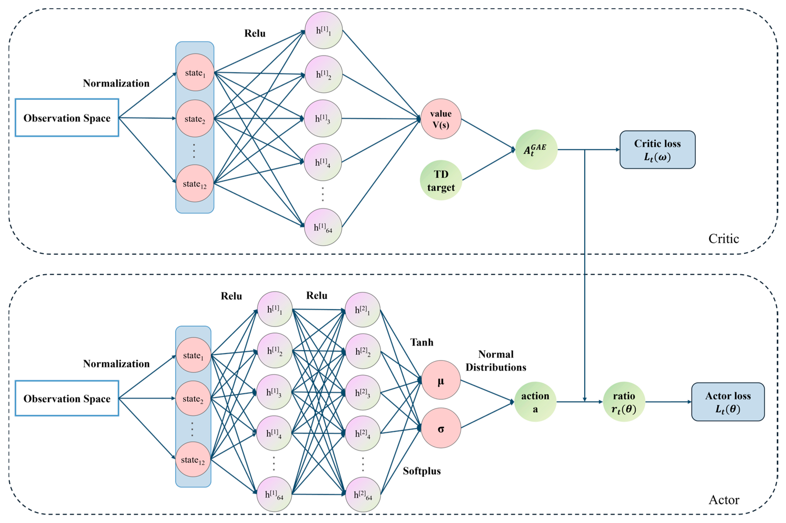
The structures of the Actor network and the Critic network are illustrated in Figure 4. The Critic network consists of a fully connected hidden layer with 64 nodes, using the Relu function as the activation function. The output is the value V ( s ) . Generalized advantage estimation A t G A E ( γ , λ ) can then be calculated with the V ( s ) and Temporal Difference target (TD target) as shown in (7), (8), and (9), where γ is the discount rate, λ is the scaling factor, δ t is the TD error at time t , and r t is the immediate reward at time t .
A t G A E γ , λ = l = 0 γ λ l δ t + l
δ t = T D   t a r g e t V s t
T D   t a r g e t = r t + γ V s t + 1
The loss for the Critic network can be defined as shown in (10). During the training process, the Critic network is updated to minimize the mean of L t ω .
L t ω = 1 2 T D   t a r g e t V s t 2
The Actor network consists of two fully connected hidden layers, each with 64 nodes and using the Relu function as the activation function. The Actor network produces two outputs: the mean μ and the standard deviation σ . The output μ uses the Tanh activation function, while the output σ uses the Softplus activation function. These values are then input into the normal distribution Formula (11) to generate the action probability distribution, determining the output action space.
f x = 1 σ 2 π e x μ 2 2 σ 2
To compute the loss function for the Actor network, PPO-Clip employs the clipped surrogate objective shown in (12), where r t ( θ ) is the probability ratio of the new policy to the old policy at time t . ε is a truncation constant that helps set the range of policy updates. During PPO training, the Actor network is updated to maximize the mean of L t ( θ ) .
L t θ = min r t θ A t , c l i p r t θ , 1 ε , 1 + ε A t
r t θ = π θ a t s t π θ o l d a t s t

3.2. Design of Observation Space and Action Space

In order to achieve trajectory planning for the airship, it is necessary to appropriately define the observation space and the action space, ensuring the airship can effectively perceive the environment, make decisions, and execute appropriate control actions.

3.2.1. Observation Space

The airship primarily acquires observation space information from two aspects, including the airship’s state information and the environmental information. After normalization, the observation is fed into the neural network. The observation space settings for the airship are shown in Table 1.
In actual flight, sensors cannot accurately measure the wind speed and direction. We considered the uncertainty in wind speed estimation during the flight. During training, we added noise with a mean of 0 and a root mean square error of 2 m/s to the observed wind speed. For the observed wind direction, we applied first-order Markov noise with a time constant of 10 min and a noise amplitude of 5°.
In assuming that the center of the station-keeping area is ( x s , y s ) , and the coordinate of the airship at time t is ( x g , y g ) , the distance to the station-keeping area center is given by the Euclidean distance
d = x s x g 2 + y s y g 2
The angle between the line from the airship to the station-keeping area center and the x-axis can be calculated as
φ = a r c t a n y s y g x s x g
Let b = { 0 ,   1 } determine whether the airship is in the station-keeping area. In assuming that the radius of the station-keeping area is r , it can be defined as follows:
b = 1 , i f   d r b = 0 , i f   d > r  

3.2.2. Action Space

According to the maneuverability of airship, the acceleration ability and turning ability of the airship were selected as the action space. Acceleration ability refers to the increase in airspeed by increasing thrust, and the dimension is the same as acceleration. The turning ability is the airship being able to change the direction of flight by turning, and the dimension is consistent with the angular velocity. Therefore, the action space is defined by acceleration and angular velocity. The specific action space settings are shown in Table 2.

3.3. Reward Design

For DRL, the design of the reward function is particularly important. In this study, the reward function consists of four components: distance reward r d , station-keeping reward r s , time reward r t , and velocity reward r v .
During the flight, in order to encourage the airship to fly towards the station-keeping area, a distance reward is given. The distance reward is defined as
r d = e r d + r
The primary goal of the flight mission is for the airship to achieve long-term regional station-keeping. Therefore, a relatively large positive reward is given for staying within the area, while a relatively large negative reward is given for being outside the area. The station-keeping reward is defined as
r s = 1 , i f   b = 1 r s = 1 ,   i f   b = 0
In order for the airship to achieve long-endurance flight, the time reward is defined as
r t = 1
Additionally, to minimize energy consumption, the airship is encouraged to maintain a lower speed. Therefore, the reward decreases as the speed increases, and the velocity reward is defined as
r v = e 0.06 v a
In these reward functions, the distance reward and station-keeping reward are the primary rewards and should be ensured to be of the same order of magnitude. The time reward and velocity reward are auxiliary rewards and should also be kept in the same order of magnitude. The primary rewards are approximately ten times those of the auxiliary rewards. This can be achieved by adjusting the weights of the rewards. The total reward function is expressed as
r = w d r d + w s r s + w t r t + w v r v     s . t .     w d + w s + w t + w v = 1
To maintain consistency among the different rewards, the weights are set as w d = 0.210 ,   w s = 0.702 ,   w t = 0.070 ,     a n d   w v = 0.018 .

4. Experiment

4.1. Traning

Our experiments were conducted on an Ubuntu 20.04 operating system, with an NVIDIA Tesla A40 GPU, an Intel Xeon Silver 4214R CPU, and Python version 3.11. Training one episode took approximately 10 min.
The basic training process is shown in Figure 5. First, the parameters of the Actor network and the Critic network are initialized to build the continuous PPO model. The training parameters were selected using grid search. We performed multiple experiments with combinations of learning rates in the range [0.0001, 0.001, 0.01] and batch sizes in [32, 64, 128]. The experimental results showed that the best training performance was achieved with an Actor learning rate of 0.0001, a Critic learning rate of 0.001, and a batch size of 32. The agent selects actions based on the normal distribution output of the Actor network. The Critic network evaluates these actions by assessing the reward obtained from executing the actions and returns the next state. This process loops until the termination condition is met. In this study, the termination conditions for the airship’s flight training environment are either the airship flying out of the training area or exceeding the maximum flight time. After each episode, the model’s convergence is checked. If the model has not converged, the parameters of the Actor network and the Critic network are updated, and training continues until convergence is achieved. Finally, the parameters of the Actor network and the Critic network are saved.
The training parameters are shown in Table 3. The total number of training steps was set to 10,000. A 7° × 7° area within a specific latitude and longitude range was selected as the training area, and training was conducted in a time-varying dynamic wind field. The wind field data were sourced from ERA5 reanalysis data, with a spatial resolution of 0.25° × 0.25°, a temporal resolution of 1 h, and a pressure level of 50 hPa. To ensure that the model adequately learned the environmental features, the starting points and station-keeping areas were randomly generated within the training area, and the station-keeping area radius was set to 25 km.
Due to the high average wind speeds from June to September (particularly in July and August), which usually exceed the airship’s maximum wind resistance, the training wind field data should avoid this period, as the model cannot be adequately trained during this time. Therefore, wind field data from 00:00 UTC, 1st December 2021 to 23:00 UTC, 30 April 2022 were selected for training. The initial flight time is randomly generated from the time range of the wind field data. Each time step is 1 min, during which the airship selects an action based on the policy to determine the next position. Spatially, we use the nearest neighbor grid point method to obtain the wind field information at that position, that is, the grid point nearest to the current airship position is selected as a reference. Temporally, we also use the nearest neighbor method by selecting the wind field data point closest to the current time point to acquire the wind field information for that moment.
The training results obtained are shown in Figure 6. When the reward curve stabilized over time, the model was considered to have converged, and the training process was manually paused. In this study, when the training reached 2000 steps, the reward curve remained stable over a period of time, indicating that the model had converged, and the training process was paused. Figure 6a shows the total reward curve during the training process. After 250 steps, the total reward gradually increases and tends to converge. Figure 6b illustrates the total flight time of the airship during the training process, and the maximum flight time is 10 days.

4.2. Testing

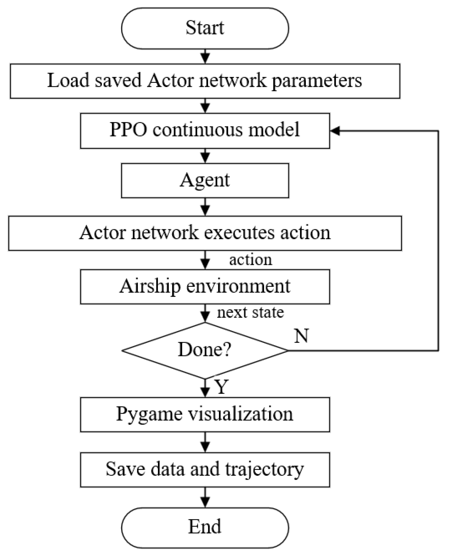
To test the generalization performance of the model, we used the saved training parameters of the Actor network to conduct monthly flight tests using the wind field data for the entire years of 2022 and 2023 in the same region. During the testing process, the station-keeping area was fixed, and the starting points were randomly generated within the test area. All take-off times were uniformly set to 00:00 UTC on the 1st of each month, with a maximum flight duration of one month. The specific testing procedure is illustrated in Figure 7.
To analyze the training results in detail, the following indicators are defined:
  • Take-off Time (TT): The take-off time of the airship, uniformly set to the 1st of each month at 00:00 UTC.
  • Flight Time (FT): The flight time of the airship within the 7° × 7° mission area.
  • Time to Reach the Station-keeping Area (TRSA): The time it takes for the airship to first reach the boundary of the station-keeping area from the starting point.
  • Station-keeping Time (ST): The total time the airship spends within the station-keeping area.
  • Station-keeping Time Ratio (STR): The ratio of the airship’s station-keeping time to its flight time.
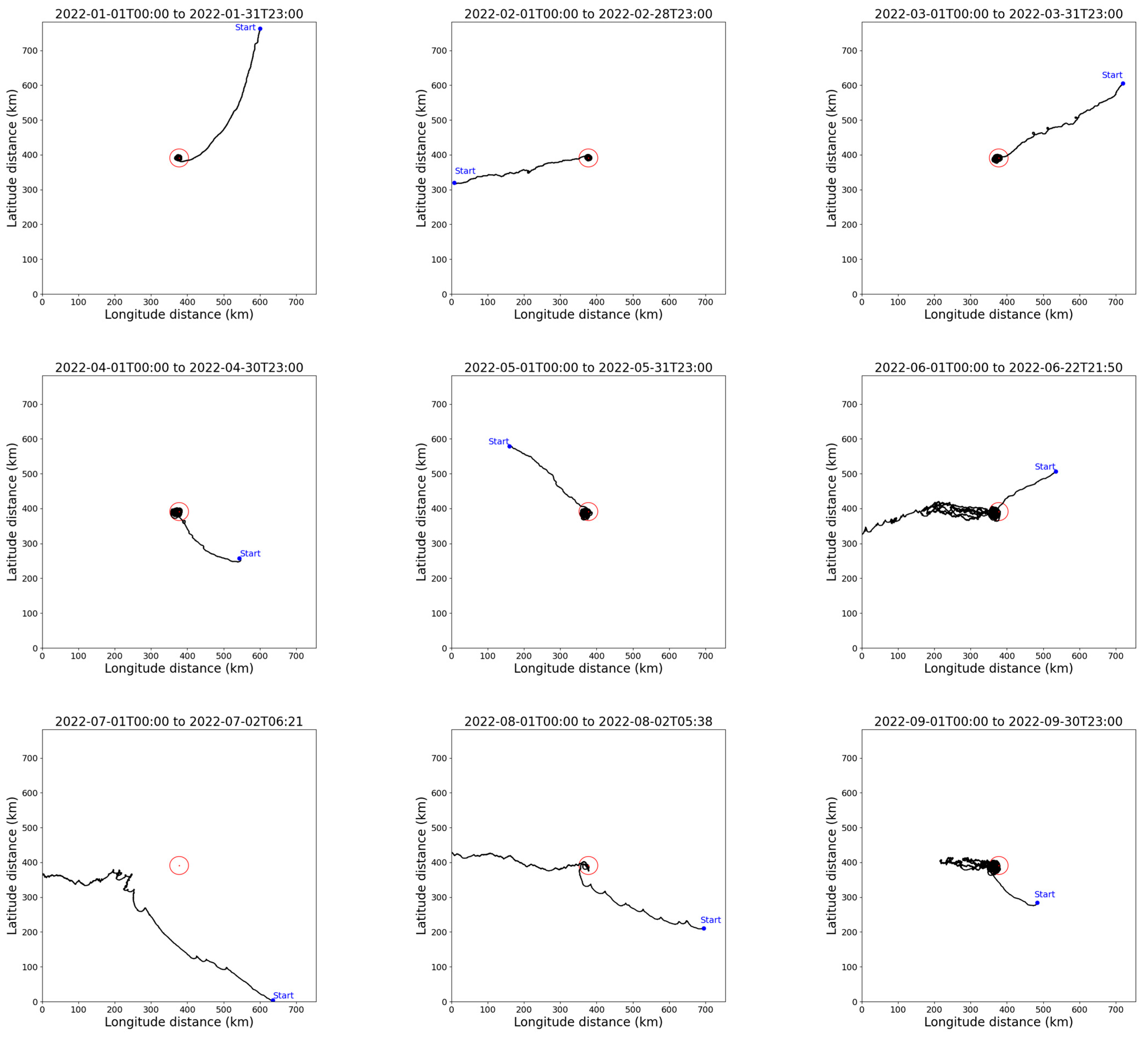
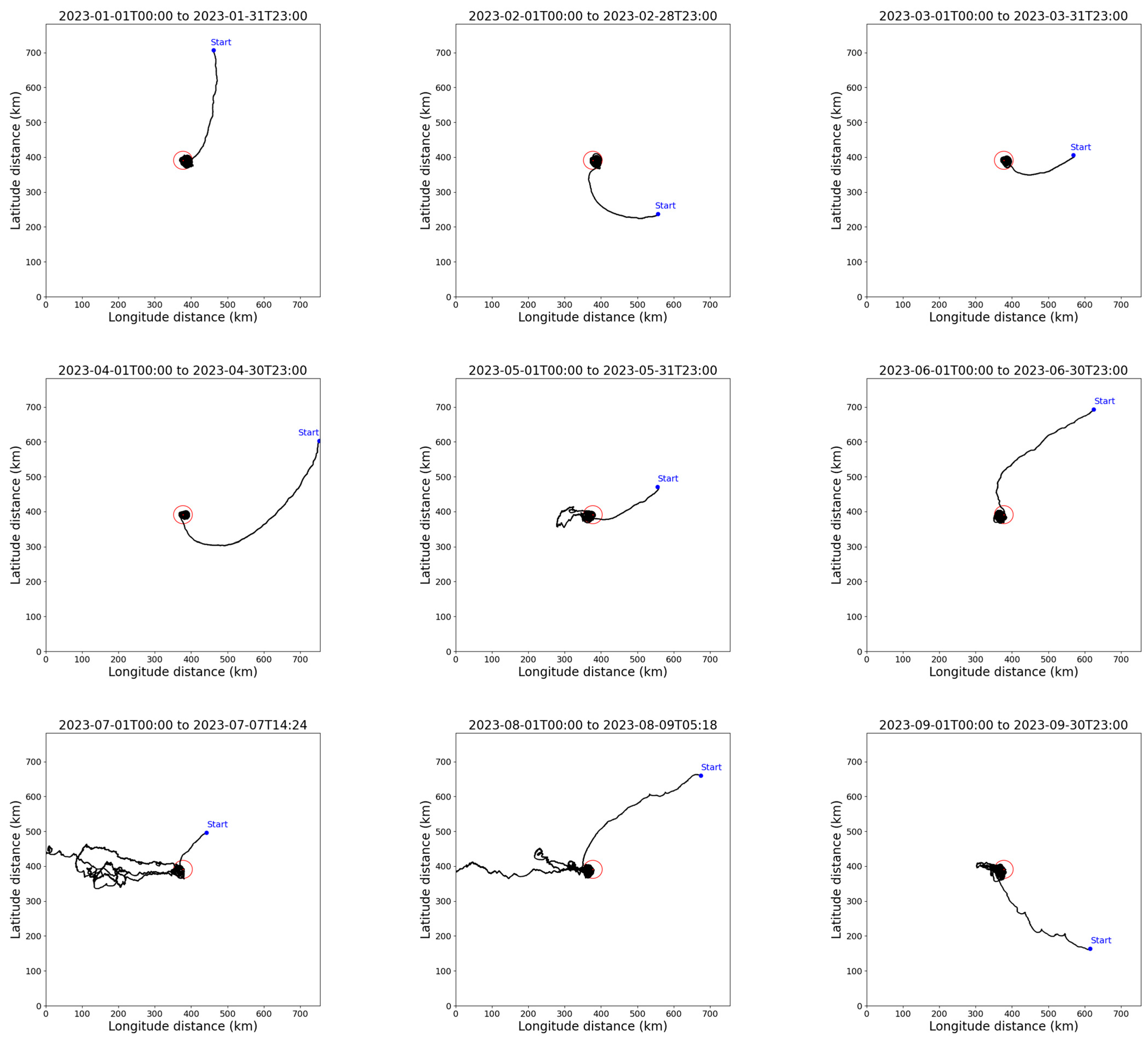
The test results are shown in Table 4, Figure A1 and Figure A2. Table 4 presents the main flight data of the airship, and Figure A1 and Figure A2 show the airship’s test flight trajectories for each month in 2022 and 2023. According to the test results, we can analyze the following aspects:
  • The influence of wind field on station-keeping performance
For July and August, the average wind speed was high, exceeding the airship’s maximum wind resistance capability, preventing the airship from maintaining long-term station-keeping. In July 2022, the airship was blown out of the flight area before entering the station-keeping area, although it showed a tendency to drift towards the station-keeping area. In August 2022, the airship was blown out of the area after staying in the station-keeping area for 0.5 days. In July and August 2023, the airship was repeatedly blown out of the station-keeping area after entering it, eventually leaving the flight area, with a maximum flight time of 8.2 days.
For June and September, the average wind speed was smaller compared to July and August. In June 2022, the airship was blown out of the flight area after flying for 21.9 days. In September 2022, June 2023, and September 2023, the airship could return to the station-keeping area after being blown out and maintain station-keeping for the entire month.
For other months, the airship could achieve effective station-keeping, with a station-keeping time ratio close to 1.0, and the maximum station-keeping time ratio was 0.997.
2.
Model performance analysis
The test results indicate that the airship can achieve long-term station-keeping in most months, proving the feasibility of the model. For months with higher wind speeds, the model still showed a tendency to drift towards the station-keeping area after being blown out. When the wind speed did not exceed the airship’s maximum wind resistance capability, the airship could autonomously return to the station-keeping area after drifting away. Additionally, the model trained on six months of wind field data can be validated for other months, further demonstrating the model’s robustness. Finally, in using wind field data from different years for testing, as shown in Table 4, the flight test results for June to September were poor, with a minimum station-keeping time ratio of 0. For other months, the airship achieved long-term station-keeping for the entire month, with the station-keeping time ratio close to 1.0. The test results for both years were consistent, proving the model’s generalization capability.
3.
Model autonomy analysis
In this study, the behavior of the airship in the wind field does not rely on past or future wind field states. During each training step, the airship only needs to know the current wind speed, position, heading, airspeed, and angular velocity to calculate the next flight trajectory, ensuring high autonomy. The system can automatically adjust and optimize the flight path based on real-time wind speed information in the current environment. In practical applications, wind speed information at the current moment can be obtained through wind speed sensors, and the system can respond to changes in wind speed in real time, without relying on previous data or predicted future wind field information.
4.
Analysis of potential sources of error
The main sources of error in the testing process include three aspects. First is the discrepancy between the actual variations in the wind field of the real world and the digital world based on reanalysis data. Considering the broad adaptability of the PPO algorithm, this error may result in a slight reduction in the actual performance, but it is still considered within a reasonable range. Second, there is the difference due to excessive simplification compared to the actual system. This paper focuses primarily on the guidance layer, but the actual tracking of airspeed and heading angles relies on the flight control system, and the real control effects may vary with different airships and control systems. Third, there is the difference between measured and estimated states and the true states. This part mainly concerns the estimation of wind fields and airspeed, which could introduce the largest errors. In practical implementation, it is crucial to improve the accuracy of these state estimations.

5. Conclusions

This paper presents an autonomous trajectory planning algorithm for stratospheric airships based on DRL. The objective is to leverage DRL’s learning capabilities to enable the airship to adapt to complex wind field variations and utilize the wind field to achieve position control, thereby ensuring long-term regional station-keeping. Through properly setting the reward function, state space, and action space, the model effectively maintains regional station-keeping under time-varying wind field conditions. The proposed method has the following notable features:
  • The model does not rely on past or future wind field states; it autonomously calculates and adjusts flight paths based on the current wind field conditions to achieve station-keeping, thereby reducing the need for manual intervention. In practical applications, current wind speed information can be obtained through wind speed sensors, allowing the system to respond immediately to changes in wind speed without relying on historical data or future wind field predictions.
  • The results of training and testing show that the model can achieve long-term regional station-keeping effectively under stable wind field conditions, with a maximum station-keeping time ratio of 0.997. Even in months with higher average wind speeds, which typically exceed the airship’s maximum wind resistance capability and cause the airship to leave the station-keeping area, the airship still shows a tendency to drift back towards the station-keeping area. Once the wind speeds subside, the airship can return to and continue station-keeping in the designated area.
Overall, the proposed method demonstrates good adaptability and robustness under various wind field conditions, providing an insightful solution for achieving autonomous long-term station-keeping for stratospheric airships. However, when applied to real-world scenarios, there may be uncertainties in trajectory prediction due to the difficulty of accurately estimating real wind fields, which should be taken into account in practical applications. Given the limitations of this study, future work will focus on incorporating energy balance considerations, refining the energy consumption model, and developing trajectory planning strategies under energy constraints. Additionally, before applying the algorithm, it is necessary to conduct more detailed testing, including evaluations with different data sources and testing in various locations, and to compare it with traditional trajectory planning methods to analyze the advantages of DRL-based trajectory planning approaches.

Author Contributions

Conceptualization, S.Z. and J.M.; methodology, S.Z.; software, S.L.; validation, S.Z., S.L. and J.M.; formal analysis, S.L.; investigation, S.Z.; resources, J.M.; data curation, Y.L.; writing—original draft preparation, S.L.; writing—review and editing, J.M.; visualization, Y.C.; supervision, H.S.; project administration, J.M.; funding acquisition, Y.L. All authors have read and agreed to the published version of the manuscript.

Funding

This research was funded by the National Key R&D Program of China, 2022YFB3207300. The article processing charge was funded by the Aerospace Information Research Institute.

Data Availability Statement

The data are contained within the article.

Conflicts of Interest

The authors declare no conflict of interest.

Appendix A

Figure A1. Flight trajectories simulation based on Pygame in 2022.
Aerospace 11 00753 g0a1aAerospace 11 00753 g0a1b
Figure A2. Flight trajectories simulation based on Pygame in 2023.
Aerospace 11 00753 g0a2aAerospace 11 00753 g0a2b

References

  1. Xu, Y.; Jiang, B.; Gao, Z.; Zhang, K. Fault tolerant control for near space vehicle: A survey and some new results. J. Syst. Eng. Electron. 2011, 22, 88–94. [Google Scholar] [CrossRef]
  2. Young, M.; Keith, S.; Pancotti, A. An overview of advanced concepts for near space systems. In Proceedings of the 45th AIAA/ASME/SAE/ASEE Joint Propulsion Conference & Exhibit, Denver, CO, USA, 2–5 August 2009; p. 4805. [Google Scholar]
  3. Parsa, A.; Monfared, S.B.; Kalhor, A. Backstepping control based on sliding mode for station-keeping of stratospheric airship. In Proceedings of the 6th RSI International Conference on Robotics and Mechatronics (IcRoM), Tehran, Iran, 23–25 October 2018; pp. 554–559. [Google Scholar]
  4. Wu, J.; Fang, X.; Wang, Z.; Hou, Z.; Ma, Z.; Zhang, H.; Dai, Q.; Xu, Y. Thermal modeling of stratospheric airships. Prog. Aerosp. Sci. 2015, 75, 26–37. [Google Scholar] [CrossRef]
  5. Mueller, J.; Paluszek, M.; Zhao, Y. Development of an aerodynamic model and control law design for a high altitude airship. In Proceedings of the AIAA 3rd” Unmanned Unlimited” Technical Conference, Workshop and Exhibit, Chicago, IL, USA, 20–23 September 2004; p. 6479. [Google Scholar]
  6. d’Oliveira, F.A.; Melo, F.C.; Devezas, T.C. High-altitude platforms—Present situation and technology trends. J. Aerosp. Technol. Manag. 2016, 8, 249–262. [Google Scholar] [CrossRef]
  7. Luo, Q.C.; Sun, K.W.; Chen, T.; Zhang, Y.F.; Zheng, Z.W. Trajectory planning of stratospheric airship for station-keeping mission based on improved rapidly exploring random tree. Adv. Space Res. 2024, 73, 992–1005. [Google Scholar] [CrossRef]
  8. Wang, J.; Meng, X.; Li, C. Recovery trajectory optimization of the solar-powered stratospheric airship for the station-keeping mission. Acta Astronaut. 2021, 178, 159–177. [Google Scholar] [CrossRef]
  9. Erke, S.; Bin, D.; Yiming, N.; Qi, Z.; Liang, X.; Dawei, Z. An improved A-Star based path planning algorithm for autonomous land vehicles. Int. J. Adv. Robot. Syst. 2020, 17, 1729881420962263. [Google Scholar] [CrossRef]
  10. Wang, H.; Yu, Y.; Yuan, Q. Application of Dijkstra algorithm in robot path-planning. In Proceedings of the Second International Conference on Mechanic Automation and Control Engineering, Inner Mongolia, China, 15–17 July 2011; pp. 1067–1069. [Google Scholar]
  11. Noreen, I.; Khan, A.; Habib, Z. A comparison of RRT, RRT* and RRT*-smart path planning algorithms. Int. J. Comput. Sci. Netw. Secur. 2016, 16, 20. [Google Scholar]
  12. Li, Q.; Xu, Y.; Bu, S.; Yang, J. Smart vehicle path planning based on modified PRM algorithm. Sensors 2022, 22, 6581. [Google Scholar] [CrossRef]
  13. Luo, Q.; Wang, H.; Zheng, Y.; He, J. Research on path planning of mobile robot based on improved ant colony algorithm. Neural Comput. Appl. 2020, 32, 1555–1566. [Google Scholar] [CrossRef]
  14. Elshamli, A.; Abdullah, H.A.; Areibi, S. Genetic algorithm for dynamic path planning. In Proceedings of the Canadian Conference on Electrical and Computer Engineering, Niagara Falls, ON, Canada, 2–5 May 2004; pp. 677–680. [Google Scholar]
  15. Miao, H.; Tian, Y.C. Dynamic robot path planning using an enhanced simulated annealing approach. Appl. Math. Comput. 2013, 222, 420–437. [Google Scholar] [CrossRef]
  16. Chen, L.; Jiang, Z.; Cheng, L.; Knoll, A.C.; Zhou, M. Deep reinforcement learning based trajectory planning under uncertain constraints. Front. Neurorobotics 2022, 16, 883562. [Google Scholar] [CrossRef] [PubMed]
  17. Arulkumaran, K.; Deisenroth, M.P.; Brundage, M.; Bharath, A.A. Deep reinforcement learning: A brief survey. IEEE Signal Process. Mag. 2017, 34, 26–38. [Google Scholar] [CrossRef]
  18. Li, Y. Deep reinforcement learning: An overview. arXiv 2017, arXiv:1701.07274. [Google Scholar]
  19. Zhou, Y.; Yang, J.; Guo, Z.; Shen, Y.; Yu, K.; Lin, J.C. An indoor blind area-oriented autonomous robotic path planning approach using deep reinforcement learning. Expert Syst. Appl. 2024, 254, 124277. [Google Scholar] [CrossRef]
  20. Yang, L.; Bi, J.; Yuan, H. Dynamic path planning for mobile robots with deep reinforcement learning. IFAC-PapersOnLine 2022, 55, 19–24. [Google Scholar] [CrossRef]
  21. Chun, D.H.; Roh, M.I.; Lee, H.W.; Yu, D. Method for collision avoidance based on deep reinforcement learning with path-speed control for an autonomous ship. Int. J. Nav. Archit. Ocean. Eng. 2024, 16, 100579. [Google Scholar] [CrossRef]
  22. Teitgen, R.; Monsuez, B.; Kukla, R.; Pasquier, R.; Foinet, G. Dynamic trajectory planning for ships in dense environment using collision grid with deep reinforcement learning. Ocean. Eng. 2023, 281, 114807. [Google Scholar] [CrossRef]
  23. Guo, T.; Jiang, N.; Li, B.; Zhu, X.; Wang, Y.; Du, W. UAV navigation in high dynamic environments: A deep reinforcement learning approach. Chin. J. Aeronaut. 2021, 34, 479–489. [Google Scholar] [CrossRef]
  24. Yan, C.; Xiang, X.; Wang, C. Towards real-time path planning through deep reinforcement learning for a UAV in dynamic environments. J. Intell. Robot. Syst. 2020, 98, 297–309. [Google Scholar] [CrossRef]
  25. Aradi, S. Survey of deep reinforcement learning for motion planning of autonomous vehicles. IEEE Trans. Intell. Transp. Syst. 2020, 23, 740–759. [Google Scholar] [CrossRef]
  26. Yu, L.; Shao, X.; Wei, Y.; Zhou, K. Intelligent land-vehicle model transfer trajectory planning method based on deep reinforcement learning. Sensors 2018, 18, 2905. [Google Scholar] [CrossRef] [PubMed]
  27. Lei, X.; Zhang, Z.; Dong, P. Dynamic path planning of unknown environment based on deep reinforcement learning. J. Robot. 2018, 2018, 5781591. [Google Scholar] [CrossRef]
  28. Xie, R.; Meng, Z.; Wang, L.; Li, H.; Wang, K.; Wu, Z. Unmanned aerial vehicle path planning algorithm based on deep reinforcement learning in large-scale and dynamic environments. IEEE Access 2021, 9, 24884–24900. [Google Scholar] [CrossRef]
  29. Ni, W.; Bi, Y.; Wu, D.; Ma, X. Energy-optimal trajectory planning for solar-powered aircraft using soft actor-critic. Chin. J. Aeronaut. 2022, 35, 337–353. [Google Scholar] [CrossRef]
  30. Zhu, G.; Shen, Z.; Liu, L.; Zhao, S.; Ji, F.; Ju, Z.; Sun, J. AUV dynamic obstacle avoidance method based on improved PPO algorithm. IEEE Access 2022, 10, 121340–121351. [Google Scholar] [CrossRef]
  31. Josef, S.; Degani, A. Deep reinforcement learning for safe local planning of a ground vehicle in unknown rough terrain. IEEE Robot. Autom. Lett. 2020, 5, 6748–6755. [Google Scholar] [CrossRef]
  32. Zheng, B.; Zhu, M.; Guo, X.; Ou, J.; Yuan, J. Path planning of stratospheric airship in dynamic wind field based on deep reinforcement learning. Aerosp. Sci. Technol. 2024, 150, 109173. [Google Scholar] [CrossRef]
  33. Yang, X.; Yang, X.; Deng, X. Horizontal trajectory control of stratospheric airships in wind field using Q-learning algorithm. Aerosp. Sci. Technol. 2020, 106, 106100. [Google Scholar] [CrossRef]
  34. Nie, C.; Zhu, M.; Zheng, Z.; Wu, Z. Model-free control for stratospheric airship based on reinforcement learning. In Proceedings of the 2016 35th Chinese Control Conference (CCC), Chengdu, China, 27–29 July 2016; IEEE: Piscataway, NJ, USA, 2016; pp. 10702–10707. [Google Scholar]
  35. Zhang, Y.; Yang, K.; Chen, T.; Zheng, Z.; Zhu, M. Integration of path planning and following control for the stratospheric airship with forecasted wind field data. ISA Trans. 2023, 143, 115–130. [Google Scholar] [CrossRef]
  36. Climate Data Store. Available online: https://cds.climate.copernicus.eu (accessed on 1 November 2023).
  37. Schulman, J.; Wolski, F.; Dhariwal, P.; Radford, A.; Klimov, O. Proximal policy optimization algorithms. arXiv 2017, arXiv:1707.06347. [Google Scholar]
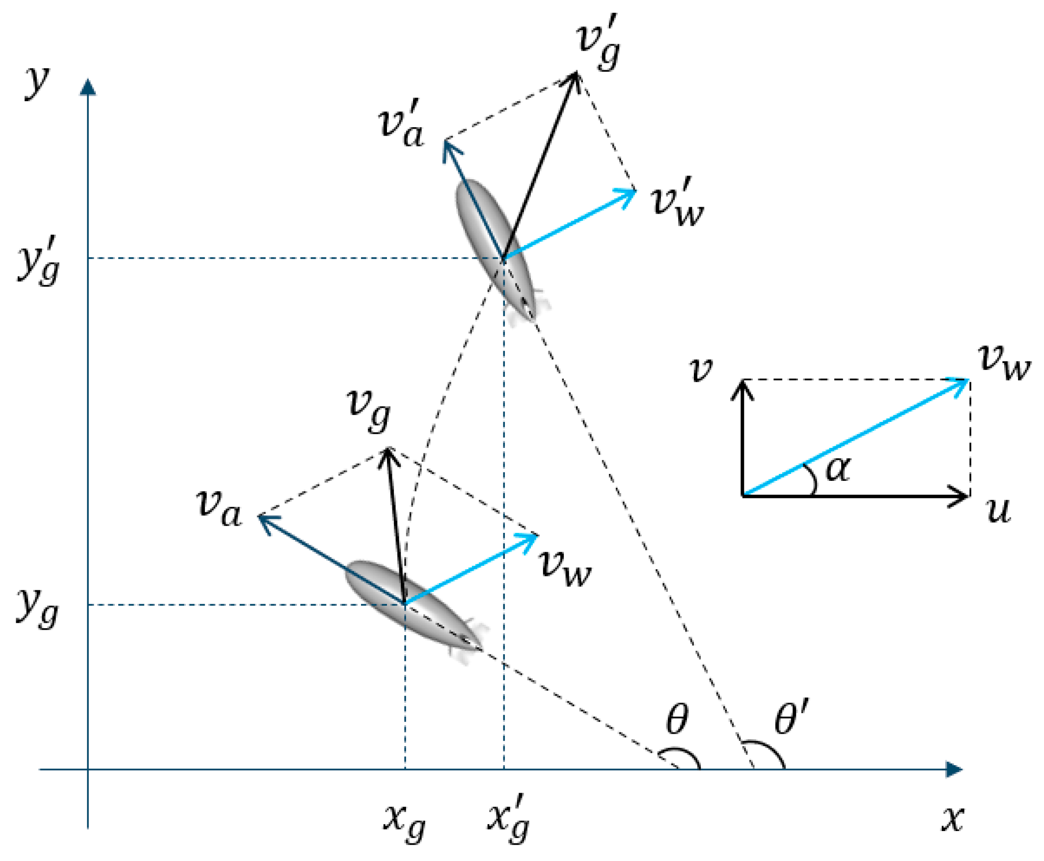
Figure 1. Displacement of airship in uncertain wind field environment.
Aerospace 11 00753 g001
Figure 2. Displacement generated by the airship’s own driving force.
Aerospace 11 00753 g002
Figure 3. The minimum, maximum, and average monthly wind speeds for typical region at 10° N latitude.
Aerospace 11 00753 g003
Figure 4. Structure of the Actor network and the Critic network.
Aerospace 11 00753 g004
Figure 5. Flow chart of training process.
Aerospace 11 00753 g005
Figure 6. Results of training process. (a) Reward changes over training steps; (b) duration changes over training steps.
Aerospace 11 00753 g006
Figure 7. Flow chart of testing process.
Aerospace 11 00753 g007
Table 1. Observation spaces of the airship.
Observation SpaceNotationMinMax
Airspeed of the airship (m/s) v a 020
Heading of the airship θ 0 2 π
Wind speed v w 0-
Wind direction α 0 2 π
Angle between the wind direction and the airspeed direction β 0 2 π
Distance between the airship and the station-keeping area center (km) d 0-
Whether present in the station-keeping area b 01
Angle between the airship to the station-keeping area center line and the x-axis φ 0 2 π
Table 2. Action spaces of the airship.
Action SpaceNotationMinMax
Acceleration (m/s2) a −0.30.15
Angular velocity (rad/s) ω −0.01250.0125
Table 3. Parameters setting.
ParametersValue
Actor learning rate 1 × 10 4
Critic learning rate 1 × 10 3
State dimension12
Action dimension2
Hidden layer dimension64
Gamma   γ 0.99
Lambda   λ 0.95
Epsilon   ε 0.2
Epoch10
Batch size32
Time step interval1 min
OptimizerAdam
Table 4. Results of testing process in 2022 and 2023.
TTFT (Days)TRSA (Min)ST (Days)STR
Year20222023202220232022202320222023
01-01 00:0031.031.042726530.730.50.9900.985
02-01 00:0028.028.039036427.727.70.9900.991
03-01 00:0031.031.038120430.730.80.9910.995
04-01 00:0030.030.022556929.829.60.9950.987
05-01 00:0031.031.024416830.830.10.9940.971
06-01 00:0021.930.010135117.329.70.7920.990
07-01 00:001.36.607102.300.343
08-01 00:001.28.23423660.55.20.4440.636
09-01 00:0030.030.090731226.428.30.8800.944
10-01 00:0031.031.040474830.530.40.9860.983
11-01 00:0030.030.011835129.929.70.9970.992
12-01 00:0031.031.035645430.630.60.9900.990
Disclaimer/Publisher’s Note: The statements, opinions and data contained in all publications are solely those of the individual author(s) and contributor(s) and not of MDPI and/or the editor(s). MDPI and/or the editor(s) disclaim responsibility for any injury to people or property resulting from any ideas, methods, instructions or products referred to in the content.