Article

Statistical Metamodel of Liner Acoustic Impedance Based on Neural Network and Probabilistic Learning for Small Datasets

1
University Gustave-Eiffel, MSME UMR 8208, 5, Boulevard Descartes, CEDEX 2, 77454 Marne-la-Vallée, France
2
Airbus Operations SAS, 31300 Toulouse, France
*
Author to whom correspondence should be addressed.
Aerospace 2024, 11(9), 717; https://doi.org/10.3390/aerospace11090717
Submission received: 30 May 2024 / Revised: 27 August 2024 / Accepted: 29 August 2024 / Published: 2 September 2024
(This article belongs to the Section Aeronautics)

Abstract

:
The main novelty of this paper consists of presenting a statistical artificial neural network (ANN)-based model for a robust prediction of the frequency-dependent aeroacoustic liner impedance using an aeroacoustic computational model (ACM) dataset of small size. The model, focusing on percentage of open area (POA) and sound pressure level (SPL) at a zero Mach number, takes into account uncertainties using a probabilistic formulation. The main difficulty in training an ANN-based model is the small size of the ACM dataset. The probabilistic learning carried out using the probabilistic learning on manifolds (PLoM) algorithm addresses this difficulty as it allows constructing a very large training dataset from learning the probabilistic model from a small dataset. A prior conditional probability model is presented for the PCA-based statistical reduced representation of the frequency-sampled vector of the log-resistance and reactance. It induces some statistical constraints that are not straightforwardly taken into account when training such an ANN-based model by classical optimizations methods under constraints. A second novelty of this paper consists of presenting an alternate solution that involves using conditional statistics estimated with learned realizations from PLoM. A numerical example is presented.

1. Introduction

We are interested in aircraft noise in the context of green aviation. This includes both external and internal noise relative to the aircraft for certification purposes. In modern turbofan engines, especially those with an ultra-high bypass ratio (UHBR), fan noise is a major contributor to overall noise. Fan noise comprises broadband and tonal noise. To attenuate the tonal noise component, particularly at a blade passing frequency (BPF), targeted acoustic liners are used, while modifications to the liners’ geometry and intrinsic properties help dissipate the broadband noise component. For effectiveness, it is crucial to study liners under various operating conditions, including different flight scenarios. The design of liners is critically important and has been extensively studied (see [1,2,3,4,5,6,7]). Liner acoustic impedance can be calculated by using an aeroacoustic computational model (ACM), which is a computationally expensive and prohibitive high-fidelity computational model for optimizing aeroacoustic performances of liners using a numerical optimization solver. Such ACMs have been developed to predict liner performance, as detailed in [8,9,10,11,12,13]. An uncertain ACM of the liner system, which allows for quantifying uncertainties in aeroacoustic models of liner performance, was also developed in [6].
The objective of this paper is to construct a statistical metamodel for which the outputs are the frequency-sampled impedance of the liner and the inputs are the control parameters that are the design parameters. The metamodel should have a low computational cost to enable its usage in optimization of liners’ aeroacoustic performance via a numerical optimization solver. In addition, the gradients of the metamodel with respect to its inputs (the control parameters) should also have a low computational cost.
In this paper, we construct the metamodel using a dataset, referred to as the ACM dataset, which includes samples of control parameters and the corresponding acoustic impedance, numerically simulated with the ACM. Consequently, the dataset is small due to the prohibitive computational cost of the ACM, which prevents the construction of a large dataset.
As only the components of the control parameter are inputs to the metamodel, all other ACM parameters are unobserved (thus uncontrolled) and should be treated as random latent variables. Therefore, the liner acoustic impedance at any frequency should also be modeled as a random variable. A first novelty contribution of this paper is the methodology for constructing such a statistical metamodel that is driven by the physics contained in the small ACM dataset.
In this paper, the statistical metamodel is defined by the conditional probability distribution of the frequency-sampled vector of the random acoustic impedance at sampled frequencies, given the control parameter. The MaxEnt principle, applied with the available information, is used to construct an informative prior model of this conditional probability distribution. It should be noted that the hyperparameters of the probabilistic model depend on the values of the control parameter and are modeled using fully connected feedforward neural networks, yielding a statistical ANN-based metamodel. Such a statistical ANN-based metamodel is fitted on an ad hoc training dataset using the maximum likelihood principle.
Principal component analysis (PCA) is conducted on the outputs (frequency-sampled acoustic impedance) of the metamodel. This is not only carried out for a potential statistical reduction but also because decorrelation and centering of outputs enhance numerical conditioning, thereby facilitating the optimization process for fitting such a statistical ANN-based model to the training dataset. However, such a statistical decorrelation and centering of the outputs introduce constraints on the hyperparameters of the statistical metamodel and, consequently, on the parameters of the statistical ANN-based metamodel. Therefore, given that these hyperparameters are modeled by fully connected feedforward networks, some deterministic constraints must be considered, yielding the development of constrained training algorithm for such networks. Such a constrained training algorithm is challenging and complex when dealing with mini-batches, and might rely on techniques such as Lagrange multipliers, penalization approaches, correction formulations, etc. A second novelty of this paper is the presentation of an unconstrained formulation for a statistical ANN-based metamodel that takes into account the statistical constraints arising from the PCA-based reduction. This is achieved by generating an ad hoc training dataset using probabilistic learning on manifolds [14,15,16,17] and using the learned dataset for estimating conditional statistics in a nonparametric framework, based on the Gaussian kernel density estimation (GKDE) method. Finally, the statistical metamodel can be used to generate additional realizations of the frequency-sampled acoustic impedance vector, thereby mitigating missing data in the set of control parameters. Compared to a previous work [18], this ANN-based surrogate model is actually a complement. First, it does not require the training dataset for offline use, significantly reducing memory requirements. Second, it allows for more efficient computation of gradients with respect to input parameters, which is crucial for optimization problems.
Note that the objective of this paper is not to improve the ANN algorithms but is to present a novel methodological application of ANNs to probabilistic ACM datasets for aeroacoustic liner impedance simulations. The novelty lies in how ANNs are used to model the hyperparameters of the probabilistic model (Section 4.1 and Section 4.2) and in how to train this model using a learned GKDE-based estimates’ dataset by PLoM (Section 4.3). This approach allows us to effectively deal with a small and probabilistic dataset, which is a significant challenge in this field and has not been widely addressed in the literature yet.
This paper is organized as follows: (1) Section 2 briefly defines the control parameters and the ACM for calculating the frequency-sampled vector of acoustic impedance, which is to be used for constructing the ACM dataset (small size). (2) Section 3 is dedicated to the parametric probabilistic modeling of the conditional probability distribution of the frequency-sampled vector of acoustic impedance, given the control parameter. (3) Section 4 focuses on the statistical ANN-based metamodel, given the control parameter. (4) Section 5 presents a numerical example, along with a discussion of the results.

2. Control Parameters and ACM Dataset

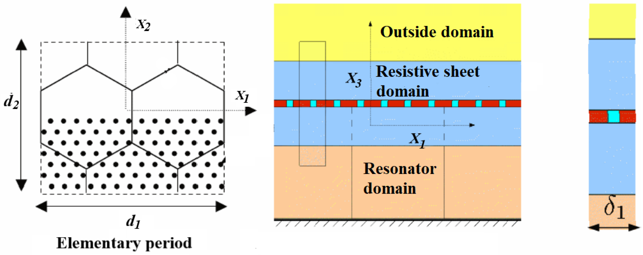
In this paper, the considered system is an acoustic liner consisting of a perforated plate, a honeycomb structure, and a rigid backing plate, as depicted in Figure 1. The Mach number is assumed to be equal to zero, which is relevant for the ground configuration. Incorporating non-zero Mach numbers requires additional analyses beyond the scope of this paper. A reduced domain, as described in [8], is used for the computational model (see Figure 2). In this paper, and for sake of simplicity, the liner system is parameterized by n w = 2 parameters (the control parameters) that are the percentage of open area (POA) and the sound pressure level (SPL), represented by w = ( w 1 , w 2 ) , where w 1 corresponds to the POA and w 2 to the SPL.
For such a reduced domain, the frequency-dependent acoustic impedance is denoted as ω z acm ( ω ; w ) , where ω is the frequency (rad/s). Specifically, z acm ( ω ; w ) = r acm ( ω ; w ) + ι v acm ( ω ; w ) , in which r acm ( ω ; w ) represents the resistance that is positive, v acm ( ω ; w ) the reactance that is real, and ι = 1 . Control parameter w belongs to an admissible set. The computational domain is centered around the resonator, within which the Navier–Stokes equations are solved. The computational model consists of 278,514 degrees of freedom. For given control parameter w , and for each sampled frequency ω k = ( k 1 ) Δ ω with k = 1 , , n w where n ω = 7 , the ACM computes the resistance r acm ( ω k ; w ) and the reactance v acm ( ω k ; w ) . The Navier–Stokes equations are solved using the numerical method presented in [8] for w = ( w 1 , w 2 ) 0.03 , 0.1 × 130 , 145 . As discussed in [18], ACM simulations are performed for n d = 48 values w 1 , , w n d of w , which constitute the set D w . These points in D w are considered as realizations of a random vector W whose probability density function, p W , is unknown.
The ACM dataset D acm is then defined as the set of points ( w j , r acm , j , v acm , j ) in R n w × n ω × n ω for j = 1 , , n d , in which r acm , j = ( r acm ( ω 1 ; w j ) , , r acm ( ω n ω ; w j ) ) and v acm , j = ( v acm ( ω 1 ; w j ) , , v acm ( ω n ω ; w j ) ) . For each j = 1 , , n d , we introduce the 2 n ω -dimensional vector of frequency-sampled impedance q acm , j = ( log r acm , j , v acm , j ) in which log r acm , j = ( log r acm ( ω 1 ; w j ) , , log r acm ( ω n ω ; w j ) ) .
The model uncertainties are due to random latent parameters that, consequently, cannot be defined as control parameters. In order to take into account these model uncertainties, the random vectors Q , R , and V are introduced, whose conditional probability density functions, given W = w j , are denoted by q p Q | W ( q | w j ) , p R | W ( r | w j ) , and p V | W ( v | w j ) . These conditional probability density functions are constructed as explained in [18]. For instance, the conditional mean value of Q given W = w j is chosen as q acm , j for j = 1 , , n d ; the conditional dispersion coefficient given W = w j is identified using experimental data. We then generate m d = 15 statistically independent realizations q j , 1 , , q j , m d from p Q | W , given W = w j . Hence, training dataset D acm is made up of a total of n acm = n d × m d realizations ( w j , k , q j , k ) with j = 1 , , n d and k = 1 , , m d , in which w j , k is a rewriting of w j that is independent of k (we introduce a repetition). For the sake of simplicity, all the realizations are rewritten as ( w j , q j ) with j = 1 , , n acm .
In [18], the PLoM (probabilistic learning on manifolds) is carried out to learn the joint probability density function p Q , W of random vectors Q and W using D acm as a training dataset. PLoM also allows n ar additional statistically independent realizations { ( w ar , q ar ) , = 1 , , n ar } to be generated, which constitute the learned dataset D ar .

3. Prior Probabilistic Model of the Frequency-Sampled Impedance Vector

In [18], the conditional probability density function p Q | W is estimated with Gaussian kernel density estimation (GKDE) using additional realizations (generated by PLoM) of Q and W . In the context of the construction of a statistical metamodel based on a neural network, we need to introduce an algebraic representation of the conditional probability distribution of Q given W , depending on hyperparameters. In this paper, we have chosen a Gaussian model for which the hyperparameters are conditional mean value and the conditional covariance matrix of Q , given W . The neural network will be used for predicting these conditional hyperparameters. In this section, we then present the construction of the algebraic priorprobabilistic model of p Q | W . Nevertheless, since Q is in a high dimension, we will introduce a statistical reduction H of Q using PCA. Within Section 3.2, the conditional hyperparameters associated with such a prior probabilistic model are represented as functions of w . The modeling of these functions is carried out using fully connected feedforward networks that are trained to map control parameter w onto a corresponding set of hyperparameters of the priorprobabilistic model.

3.1. PCA-Based Statistical Reduction H of Q

PCA is used to construct the statistical reduction of Q , yielding a normalized random vector H (centered with identity covariance matrix). Random vector H is therefore written as H = λ 1 / 2 ϕ T Q q ̲ , in which q ̲ = ( 1 / n ar ) = 1 n ar q ar is the empirical mean value of random vector Q , [ λ ] is a ( m × m ) diagonal matrix, and [ ϕ ] is a ( n q × m ) matrix whose columns are orthonormal vectors, and are such that [ C Q ] [ ϕ ] = [ ϕ ] [ λ ] . The estimate of the ( n q × n q ) covariance matrix of Q is [ C Q ] = ( n ar 1 ) 1 = 1 n ar ( q ar q ̲ ) ( q ar q ̲ ) T . The diagonal entries of [ λ ] are the m-largest eigenvalues of [ C Q ] . By construction, the R m -valued random variable H is such that
E { H } = 0 m , E { H H } = [ I m ] .

3.2. Prior Conditional Probabilistic Density Function of H Given W

Let η p H | W ( η | w ) be the conditional probability density function of H , given W . The priorconditional probability density function p H | W is constructed using the MaxEnt principle (see, for instance, [19]) with the following available information: (1) The support of η p H | W ( η | w ) is R m . (2) The conditional mean value and the conditional covariance matrix of H given W = w are the vector μ H | W ( w ) and the matrix [ C H | W ( w ) ] , which are estimated using the training dataset D ar for each given value of w . Therefore, H given W = w is a multivariate Gaussian random variable with mean value μ H | W ( w ) and covariance matrix [ C H | W ( w ) ] .
For any given w in its admissible set, the estimates of hyperparameters μ H | W ( w ) and [ C H | W ( w ) ] , constructed using GKDE from nonparametric statistics and dataset D ar , are written as
μ H | W ( w ) = = 1 n ar η ar exp 1 2 s 2 ( w w ar ) T [ C W ] 1 ( w w ar ) = 1 n ar exp 1 2 s 2 ( w w ar ) T [ C W ] 1 ( w w ar ) ,
[ C H | W ( w ) ] = = 1 n ar η ˜ ar ( w ) ( η ˜ ar ( w ) ) T exp 1 2 s 2 ( w w ar ) T [ C W ] 1 ( w w ar ) = 1 n ar exp 1 2 s 2 ( w w ar ) T [ C W ] 1 ( w w ar ) ,
where (1) the ( n w × n w ) matrix [ C W ] = ( n ar 1 ) 1 = 1 n ar ( w ar w ̲ ) ( w ar w ̲ ) T is the estimate of the covariance matrix of W in which w ̲ = ( 1 / n ar ) = 1 n ar w ar is the estimate of the mean value of W ; (2) for all = 1 , , n ar , we have η ar = [ λ ] 1 / 2 [ ϕ ] T ( q ar q ̲ ) and η ˜ ar ( w ) = η ar μ H | W ( w ) ; (3) s is the Silverman bandwidth given by
s = 4 n ar ( 2 + n ) 1 / ( n + 4 ) , n = m + n w
Due to Equation (1), μ H | W ( w ) and [ C H | W ( w ) ] have to satisfy the following equations:
E { μ H | W ( W ) } = 0 m ,
E [ C H | W ( W ) ] + μ H | W ( W ) μ H | W ( W ) T = [ I m ] .
With the proposed methodology, these two equations will automatically be satisfied.

3.3. Statistically Independent Realizations of R and V Given W

For given w , let R ( w ) and V ( w ) be the R n ω -valued random variables defined in Section 2. For any given w in its admissible set, N statistically independent realizations η 1 ( w ) , , η N ( w ) of H given W = w are generated using the multivariate Gaussian random distribution whose mean value is μ H | W ( w ) and covariance matrix is [ C H | W ( w ) ] . We then deduce N statistically independent realizations q 1 ( w ) , , q N ( w ) of random vector Q given W = w such that, for j = 1 , , N , q j ( w ) = q ̲ + [ Φ ] [ λ ] 1 / 2 η j ( w ) . For j = 1 , , N , the block decomposition of vector q j ( w ) is written as ( q R j ( w ) , v j ( w ) ) with q R j and v j ( w ) being two n ω dimensional vectors. Obviously, v 1 ( w ) , , v N ( w ) are statistically independent realizations of V ( w ) , and the statistically independent realizations r 1 ( w ) , , r N ( w ) of R ( w ) are such that q R j ( w ) = log ( r j ( w ) ) . Note that, for a given w , conditional mean vectors μ R | W ( w ) and μ V | W ( w ) , as well as the conditional covariance matrices [ C R | W ( w ) ] and [ C V | W ( w ) ] , are estimated using the statistically independent realizations r j ( w ) , , r N ( w ) and v j ( w ) , , v N ( w ) . Note that vector μ R | W ( w ) and matrix [ C R | W ( w ) ] can also be written as
μ R | W ( w ) = exp μ Q R | W ( w ) + 1 2 diag [ C Q R | W ( w ) ] ,
[ C R | W ( w ) ] = exp [ C Q R | W ( w ) ] 1 μ R | W ( w ) μ R | W ( w ) T ,
where [ A ] [ B ] stands for Hadamard product of matrices [ A ] and [ B ] ; exp ( [ A ] ) is the element-wise exponential, and diag [ A ] is the vector made up of the diagonal entries of a given matrix [ A ] . The block decomposition of μ Q | W ( w ) = q ̲ + [ Φ ] [ λ ] 1 / 2 μ H | W ( w ) into n ω dimensional vectors μ Q R | W ( w ) and μ V | W ( w ) is written as
μ Q | W ( w ) = ( μ Q R | W ( w ) , μ V | W ( w ) ) .
The block decomposition of matrix [ C Q | W ( w ) ] = [ Φ ] [ λ ] 1 / 2 [ C H | W ( w ) ] [ λ ] 1 / 2 [ Φ ] T into ( n ω × n ω ) matrices [ C Q R | W ( w ) ] , [ C ( w ) ] , and [ C V | W ( w ) ] is written as
[ C Q | W ( w ) ] = [ C Q R | W ( w ) ] [ C ( w ) ] [ C ( w ) ] [ C V | W ( w ) ] .
Concerning the random frequency-sampled vector V ( w ) , vector μ V | W ( w ) and matrix [ C V | W ( w ) ] are directly obtained from the block decomposition of vector μ Q | W ( w ) and matrix [ C Q | W ( w ) ] given by Equations (9) and (10).

4. Statistical ANN-Based Metamodel

4.1. Fully Connected Feedforward Neural Network

Deterministic mappings w μ H | W ( w ) and w [ C H | W ( w ) ] may have complex behavior, not only because their supports are multidimensional, but also because the underlying physical process is complex. In such a case, a fully connected feedforward neural network is well adapted to represent such deterministic mappings. We then consider a fully connected feedforward neural network μ H | W ( w θ 1 ) with parameter θ 1 , which is constructed in order to model deterministic mapping w μ H | W ( w ) . However, a representation of w [ C H | W ( w ) ] by a fully connected feedforward network is not straightforward because, for each given w , the output has to be a positive-definite matrix. To circumvent this apparent difficulty, the matrix logarithm of the ( m × m ) symmetric covariance matrix [ C H | W ( w ) ] is calculated for each given w , which yields a ( m × m ) symmetric matrix [ log C H | W ( w ) ] . If all the m ( m + 1 ) / 2 entries of the upper triangular block of matrix [ log C H | W ( w ) ] are collected into the m ( m + 1 ) / 2 dimensional vector ζ H | W ( w ) , then a fully connected feedforward network ζ H | W ( w θ 2 ) with parameter θ 2 is constructed for modeling the deterministic mapping w ζ H | W ( w ) . Then, for a given w , the output of ζ H | W ( w ; θ 2 ) with parameter θ 2 is used in order to assemble matrix [ log C H | W ( w ; θ 2 ) ] . Then, matrix [ C H | W ( w ; θ 2 ) ] is calculated as the matrix exponential of [ log C H | W ( w ; θ 2 ) ] . We then define the statistical ANN-based metamodel as the probabilistic model in Section 3, where μ H | W ( w ; θ 1 ) and [ C H | W ( w ; θ 2 ) ] are used for modeling μ H | W ( w ) and [ C H | W ( w ) ] . Consequently, the statistical ANN-based model is defined as the probability density function η p H | W ( η | w ; θ 1 , θ 2 ) that is a multivariate Gaussian probability density function with mean value μ H | W ( w ; θ 1 ) and covariance matrix [ C H | W ( w ; θ 2 ) ] .
This ANN-based approach is actually a complement to the model presented in [18]. The previous model relies on conditional statistics based on the PLoM generation of the learned dataset requiring the training dataset. The proposed ANN-based model, once trained, can make predictions without referencing the learned dataset, at the price of introducing a probabilistic simplification concerning the probability distributions. This feature significantly reduces the computational resources required for deployment. In addition, the ANN-based model can be viewed as another type of representation of the surrogate model in [18].

4.2. Statistical ANN-Based Metamodel for Regression with the Learned Dataset D ar

As it is usually the case for most regression problems, parameters θ 1 and θ 2 are adjusted by fitting the statistical ANN-based metamodel to a suitable training dataset. In this paper, such fitting is carried out in minimizing with respect to θ 1 and θ 2 regarding the negative-log-likelihood L ( θ 1 , θ 2 ) of the statistical ANN-based model. Obviously, D acm and D acm are not suitable as training datasets for such a fitting process since their sizes are small (less than one hundred elements). It is well known that, in the framework of statistical ANN-based modeling (as well for deterministic ANN-based modeling), small training datasets yields overfitting models that are unable to predict their targets well enough for unseen values of their inputs. On the other hand, since the size n ar of learned dataset D ar is as large as needed, such dataset is completely suitable as a training dataset. Using learned dataset D ar , the negative-log-likelihood to be minimized is written as
L ( θ 1 , θ 2 ) = = 1 n ar log p H , W ( η ar , w ar ; θ 1 , θ 2 ) ,
  = = 1 n ar log p H | W ( η ar | w ar ; θ 1 , θ 2 ) p W ( w ar ) ,
  = = 1 n ar log p H | W ( η ar | w ar ; θ 1 , θ 2 ) = 1 n ar log p W ( w ar ) .
Minimizing L ( θ 1 , θ 2 ) with respect to θ 1 and θ 2 is equivalent to minimizing the cost function J ( θ 1 , θ 2 ) , which is defined by
J ( θ 1 , θ 2 ) = 1 2 = 1 n ar log det [ C H | W ( η ar ; θ 2 ) ] + 1 2 = 1 n ar η ar μ H | W ( w ar ; θ 1 ) T [ C H | W ( w ar ; θ 2 ) ] 1 η ar μ H | W ( w ar ; θ 1 ) .
Note that such minimization should be performed under the constraints defined by Equations (5) and (6). Classically, such constraints would be taken into account by introducing Lagrange multipliers [20,21,22], augmented Lagrangian methods [21,22], penalty methods [20,21,22], barrier methods [22], projected gradient methods [23], or Sequential Quadratic Programming [22]. It is not straightforward to implement such methods in the framework of fully connected feedforward neural network training when mini-batches are required due to constraints regarding RAM availability due to CPU or GPU limitations. In this paper, and as explained in Section 4.3, we take advantage of the PLoM in order to fit the probabilistic model by adjusting θ 1 and θ 2 , such that constraints defined by Equations (5) and (6) are automatically satisfied.

4.3. Statistical ANN-Based Metamodel for Regression with a Learned GKDE-Based Estimates’ Dataset

It should be noted that minimizing J ( θ 1 , θ 2 ) with respect to θ 1 and θ 2 under constraints defined by Equations (5) and (6) is equivalent to constructing the likelihood-based statistical estimators of the conditional mean and conditional covariance matrix of H , given W = w . Such statistical estimators are different from the GKDE-based statistical estimators defined by Equations (2) and (3). Therefore, in the context of constructing μ H | W ( w ; θ 1 ) and ζ H | W ( w ; θ 2 ) , an alternative strategy to the typical approach of minimizing the negative-log-likelihood L ( θ 1 , θ 2 ) in regression problems, as presented in Section 4.2, is proposed. This alternative entails generating a GKDE-based estimates’ dataset D H | W made up of pre-calculated estimates of a conditional mean and conditional covariance of H , given W , using GKDE-based estimators as defined by Equations (2) and (3). Then, parameters θ 1 and θ 2 are adjusted such that the statistical ANN-based metamodel defined by μ H | W ( w ; θ 1 ) and ζ H | W ( w ; θ 2 ) fits dataset D H | W . Such a strategy requires a very large dataset D ar in order to construct a large enough dataset D H | W using GKDE-based estimators. Such an adapted very large dataset D ar can easily be constructed by PLoM. Therefore, dataset D H | W consists of ν < n ar elements ( μ 1 , ζ 1 ) , , ( μ ν , ζ ν ) defined as follows. For all j = 1 , , ν ,
μ j = = ν + 1 n ar η ar exp 1 2 s 2 ( w ar j w ar ) T [ C W ] 1 ( w ar j w ar ) = ν + 1 n ar exp 1 2 s 2 ( w ar j w ar ) T [ C W ] 1 ( w ar j w ar ) ,
and the m ( m + 1 ) / 2 dimensional vector ζ j collects all the entries of the upper triangular part of the matrix logarithm [ log C j ] of the matrix [ C j ] , defined as
[ C j ] = = ν + 1 n ar η ˜ ar ( w ar j ) ( η ˜ ar ( w ar j ) ) T exp 1 2 s 2 ( w ar j w ar ) T [ C W ] 1 ( w ar j w ar ) = ν + 1 n ar exp 1 2 s 2 ( w ar j w ar ) T [ C W ] 1 ( w ar j w ar ) .
Note that n ar ν is the number of realizations used for the GKDE-based estimates of the conditional mean and conditional covariance of H , given W = w ar j . Hence, the least-square estimation of parameters θ 1 and θ 2 is obtained as the parameters that minimize the cost function J ( θ 1 , θ 2 ) , written as
J ( θ 1 , θ 2 ) = j = 1 ν μ j μ H | W ( w ar j ; θ 1 ) 2 + j = 1 ν ζ j ζ H | W ( w ar j ; θ 2 ) 2 ,
This optimization problem is solved using the ADAM (ADAptive Moment estimation) algorithm [24] with a learning rate γ scheduler that adjusts the learning rate over the course of training as
γ ( k ) = max ( γ o α ( k 1 ) / Δ , γ min ) ,
where k is the epoch, γ o is the initial learning rate (default value is γ o = 0.001 ), α = 0.95 is the decay factor, Δ = 5 is the decay period, and γ min = 1 × 10 7 is the minimum leaning rate. For the ADAM algorithm, the parameters are fixed as β 1 = 0.9 , β 2 = 0.99 , and ϵ = 1 × 10 8 .

5. Numerical Applications

5.1. Architecture of the Statistical ANN-Based Metamodel

Concerning the architecture of the statistical ANN-based metamodel, rather than constructing two multi-outputs fully connected feedforward networks (one for μ H | W ( w ; θ 1 ) and one for ζ H | W ( w ; θ 2 ) ), we choose to construct m single output fully connected feedforward networks { μ H | W ( w ; θ 1 , 1 ) } 1 , , { μ H | W ( w ; θ 1 , m ) } m and d = m ( m + 1 ) / 2 single output fully connected feedforward networks { ζ H | W ( w ; θ 2 , 1 ) } 1 , , { ζ H | W ( w ; θ 2 , d ) } d , where θ 1 is rewritten as θ 1 = ( θ 1 , 1 , , θ 1 , m ) and θ 2 is rewritten as θ 2 = ( θ 2 , 1 , , θ 2 , d ) . The training is carried out in parallel on a cluster of three Tesla V100 GPUs (Nvidia, Santa Clara, CA, USA). For each fully connected feedforward network, there are four hidden layers, and the number of units is 20, 250, 75 and 25, respectively. This architecture implies a total number of 26,314 parameters (biases and weights). For the first and the fourth layer, the Glorot [25] initialization is used; for the second and third layer, the He [26] initialization is used. Rectified linear unit (ReLU) activation functions are used for each of the four hidden layers.

5.2. Statistical Convergence Analysis for the Learned GKDE-Based Estimates’ Dataset

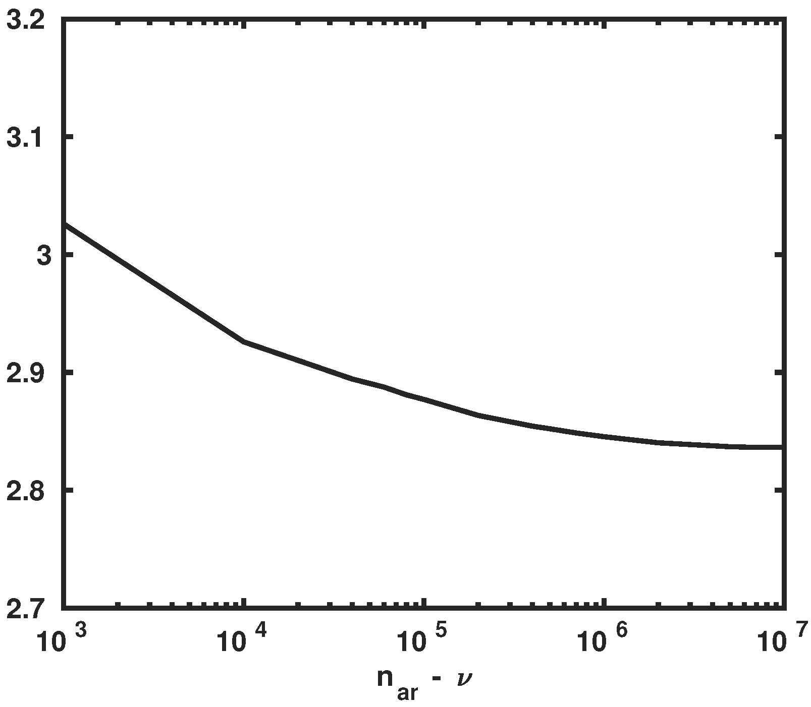
Statistical convergence analysis is carried out with respect to number ν (see Section 4.3). Figure 3 shows the graph of n ar ( n ar ν + 1 ) 1 j = ν + 1 n ar [ C H | W ( w ar j ) ] 2 in which · is the Frobenius norm. The horizontal axis of Figure 3 is the number n ar ν , which comprises statistically independent realizations used in order to construct the GKDE-based estimates of conditional covariance of H , given W = w with ν = 60,000. It can be shown that convergence is reached for n ar ν = 200,000; thus, n ar = 260,000.

5.3. Conditional Covariance Matrices of R and V Given W

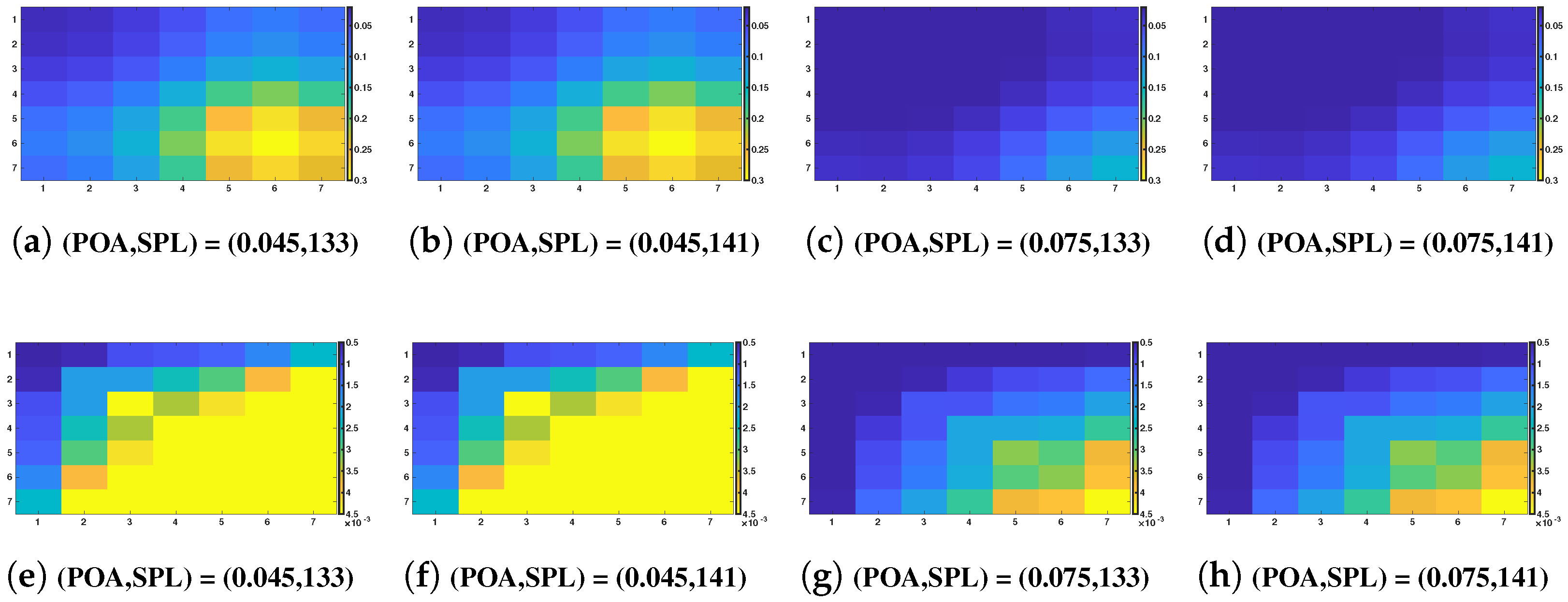
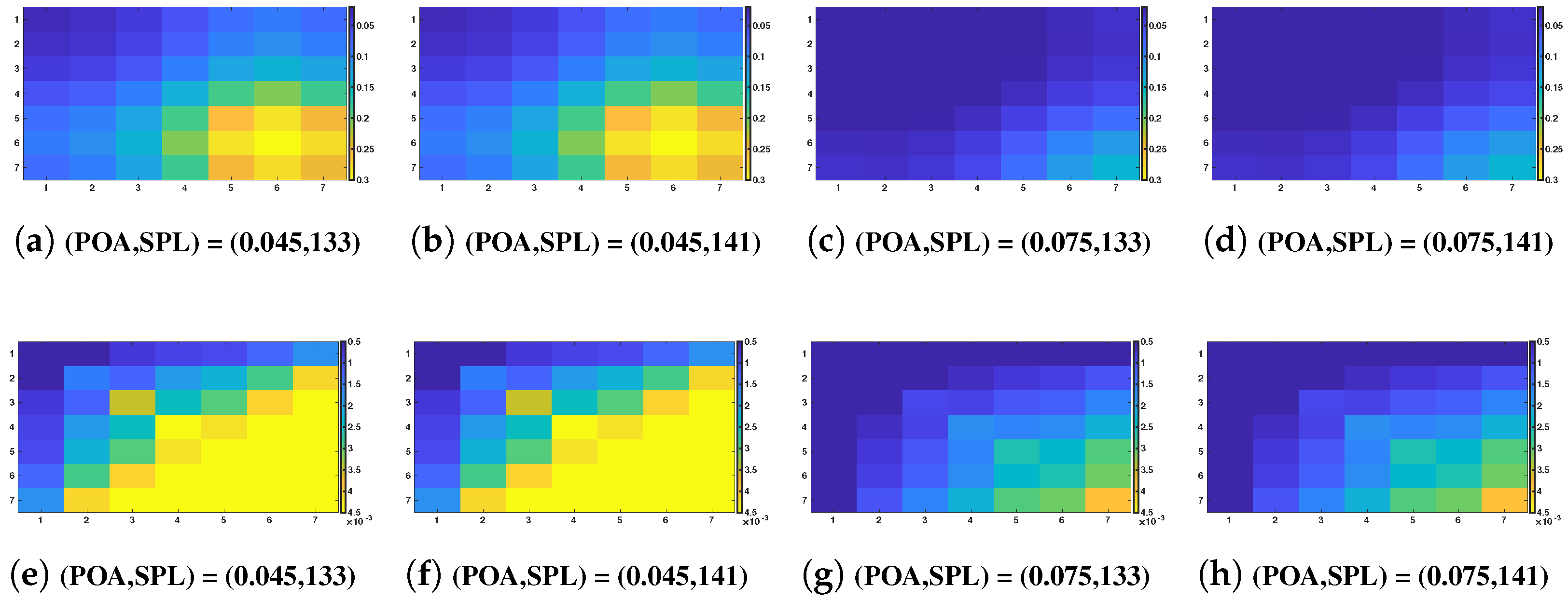
Using the database D ar and conditional statistics based on the GKDE, the ( m × m ) conditional covariance matrix [ C Q | W ( w ) ] can be calculated. The expression is not included in this paper but is similar to Equation (3) using q ar j instead of η ar j and with a Silverman bandwidth n = n q + n w in Equation (4). Using Equations (7)–(10) allow for calculating conditional covariance matrices of resistance [ C R | W ( w ) ] and reactance [ C V | W ( w ) ] for any given W = w . Furthermore, as explained in Section 3.3 and given models μ H | W ( w ; θ 1 ) and ζ H | W ( w ; θ 2 ) , the conditional covariance matrix [ C R | W ( w ; θ 1 , θ 2 ) ] (resp. [ C V | W ( w , θ 2 ) ] ) of R ( w ) (resp. V ( w ) ) can be constructed for any given W = w . The entries of matrices [ C R | W ( w ) ] and [ C V | W ( w ) ] (calculated with the GKDE) are displayed in Figure 4. The entries of matrices [ C R | W ( w ; θ 1 , θ 2 ) ] and [ C V | W ( w ; θ 2 ) ] (calculated using the statistical ANN-based metamodel) are displayed in Figure 5. The frequency-sampled resistance is displayed in Figure 4a–d and Figure 5a–d. The frequency-sampled reactance is displayed in Figure 4e–h and Figure 5e–h. It should be noted that the considered values of the control parameters are indicated in each sub-figure. It can be seen that the matrices are not diagonal and that a correlation exits between the different frequency points of the frequency-sampled impedance. It can also be seen that the GKDE-based estimate in Figure 4 and statistical ANN-based metamodel estimate in Figure 5 of the covariance matrices are quantitatively the same.

5.4. Frequency-Sampled Impedance Using the Statistical ANN-Based Metamodel

For any value of w in its admissible set, the conditional statistics (mean values and confidence regions) of R ( w ) and V ( w ) are estimated using the statistically independent realizations r 1 ( w ; θ 1 , θ 2 ) , , r N ( w ; θ 1 , θ 2 ) and v 1 ( w ; θ 1 , θ 2 ) , , v N ( w ; θ 1 , θ 2 ) , as presented in Section 3.3, and obtained using μ H | W ( w ; θ 1 ) and ζ H | W ( w ; θ 2 ) , as explained in Section 4.1.
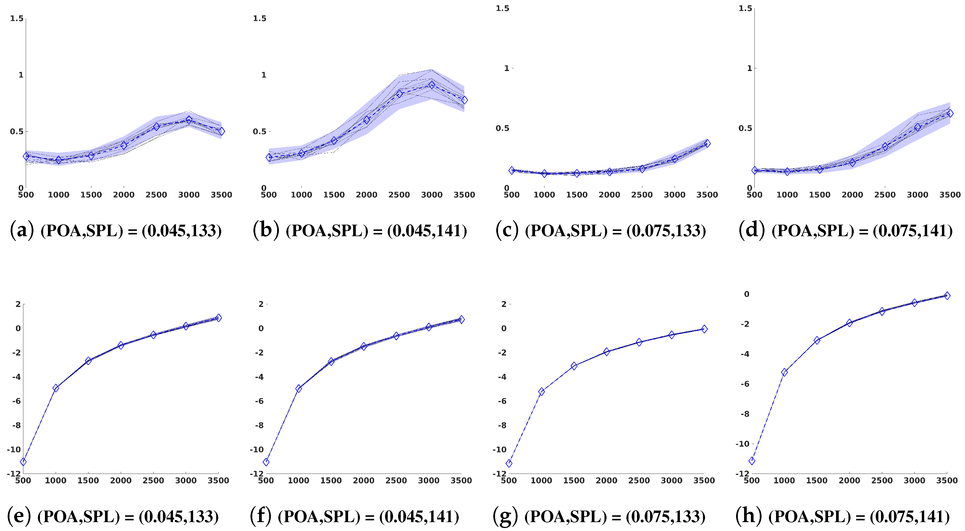
Figure 6 shows 10 realizations of frequency-sampled resistances (Figure 6a–d) and 10 corresponding realizations of frequency-sampled reactance (the values of the control parameters are indicated in each sub-figure). The dashed blue line (resp. the blue domain) is the conditional mean value (resp. the conditional confidence region) of the frequency-sampled resistance (Figure 6a–d) and reactance (Figure 6a–d).
The conditional mean value and the conditional confidence region with probability level P c = 98 % , of the frequency-sampled impedance given W = w , corresponding to the statistical ANN-based metamodel, are presented in Figure 7 and are compared with the results presented in [18] (GKDE-based estimates). Figure 7a–d correspond to the resistance, and Figure 7e–h correspond to the reactance (the values of the control parameters are indicated in each sub-figure). The red dashed line (resp. the red domain) shows the conditional mean value (resp. the confidence region) from [18]. The blue dashed line (resp. the blue domain) shows the conditional mean value (resp. confidence region) from the statistical ANN-based metamodel. It can be seen that, concerning the conditional mean values of the frequency-sampled impedance, there is a good match between the statistical ANN-based metamodel presented in this paper and the previous results presented in [18]. The statistical ANN-based metamodel, which was fitted on the learned GKDE-based estimates’ dataset D H | W (with 60,000 realizations), shows a conditional confidence region that is quantitatively the same as those calculated by the GKDE-based estimate using the learned ACM dataset D ar (260,000 realizations) with manually adjusted Silverman bandwidth s to the value 0.1186 .

6. Conclusions and Perspectives

In this paper, a statistical ANN-based metamodel of the frequency-sampled liner acoustic impedance was presented, for which only a small ACM dataset was available to fit its parameters. The control parameters were the POA and SPL, with the Mach number being kept at zero. The latent (unobserved) parameters introduce uncertainties that are taken into account by a probabilistic model introduced in [18]. The construction of the statistical metamodel used PCA to construct a statistically reduced representation of the frequency-sampled vector of the random log-resistance and the random reactance. For fitting the statistical ANN-based metamodel, a big training dataset was constructed using probabilistic learning on manifolds (PLoM). A priorconditional probability distribution of the reduced representation given the control parameters was then constructed and assumed to be Gaussian, yielding a multivariate log-normal distribution for the resistance and a multivariate Gaussian distribution for the reactance. The metamodels of the hyperparameters of such a conditional probabilistic model were presented as fully connected feedforward neural networks. As the reduced representation was modeled by a centered and normalized random vector, some constraints had to be taken into account in the minimization of the negative-log likelihood when fitting the parameters (biases and weights) of the neural network. The constrained problem was transformed into an unconstrained one, requiring the construction of a second training dataset to estimate the conditional mean vectors and conditional covariance matrices for which the learned realizations were generated using PLoM. The novelty of this paper lies in the methodology used to construct a statistical ANN-based metamodel of liner acoustic impedance, which can be used as a low-computational-cost metamodel to predict the confidence interval and the mean value of the impedance, given any value of the control parameter. The gradients of the mean values and confidence regions can also easily be derived using classical backpropagation algorithms for a very cheap computational cost. The statistical ANN-based metamodel presented in this paper is a complement to the model proposed in [18]. Firstly, it allows for offline use, as it does not require access to the learned dataset for making predictions. Secondly, the gradient computations with respect to input parameters are expected to be computationally cheaper, facilitating its use in optimization problems. These improvements, combined with the ANN’s ability to capture complex, multidimensional relationships, make this new model a flexible and efficient tool for optimizing liner acoustic impedance across the parameter space. Such work can be extended to a non-zero Mach number in the ACM dataset.

Author Contributions

Methodology, A.S., C.D. and C.S.; Software, A.S. and C.S.; Data curation, G.C.; Writing—original draft, A.S.; Writing—review & editing, C.D., C.S. and G.C.; Supervision, C.D. and C.S.; Funding acquisition, G.C. All authors have read and agreed to the published version of the manuscript.

Funding

This work was supported by DGAC (Direction Générale de l’Aviation Civile), by PNRR (Plan National de Relance et de Résilience Français), and by NextGeneration EU via the project MAMBO (Méthodes Avancées pour la Modélisation du Bruit moteur et aviOn).

Data Availability Statement

Data is contained within the article.

Conflicts of Interest

Author Guilherme Cunha was employed by the company Airbus Operations SAS. The remaining authors declare that the research was conducted in the absence of any commercial or financial relationships that could be construed as a potential conflict of interest.

Nomenclature

[ C H | W ( w ) ] Conditional covariance matrix of H given W = w
[ C Q ] Covariance matrix of Q
[ C R | W ( w ) ] Conditional covariance matrix of R given W = w
[ C V | W ( w ) ] Conditional covariance matrix of V given W = w
E { · } Mathematical expectation operator
J ( θ 1 , θ 2 ) Cost function for ANN training
n d Number of values in D w
n w Number of control parameters
n ω Number of sampled frequencies
p Q | W , p R | W , p V | W Conditional probability density functions
p W Probability density function of W
r acm ( ω ; w ) Resistance from the ACM
sSilverman bandwidth
v acm ( ω ; w ) Reactance from the ACM
μ j j-th realization of conditional mean
Q , R , V Random vectors for impedance, resistance, and reactance
q ̲ Empirical mean value of Q
q acm , j j-th frequency-sampled impedance from the ACM
q j , k k-th realization of frequency-sampled impedance given W = w j
q ar -th additional realization of frequency-sampled impedance
r acm , j j-th frequency-sampled resistance from the ACM
w = ( w 1 , w 2 ) Control parameters (POA and SPL)
w j j-th realization of control parameters
w j , k Rewriting (with repetition) of w j , k = w j
w ar -th additional realization of control parameters
W Random vector of control parameters
z acm ( ω ; w ) Frequency-dependent acoustic impedance from the ACM
ζ j j-th realization of covariance matrix parameters
[ λ ] Diagonal matrix of eigenvalues
[ ϕ ] Matrix of eigenvectors
H Normalized random vector from PCA
μ H | W ( w ; θ 1 )         ANN output for conditional mean of H given W = w
ζ H | W ( w ; θ 2 ) ANN output for vectorized upper triangular elements of the matrix logarithm of [ C H | W ( w ) ]
L ( θ 1 , θ 2 ) Negative log-likelihood
ω Frequency (rad/s)
θ 1 , θ 2 Parameters of the ANN
ACMAeroacoustic computational model
ANNArtificial neural network
BPFBlade passing frequency
GKDEGaussian kernel density estimation
MaxEntMaximum entropy
PCAPrincipal component analysis
PLoMProbabilistic learning on manifolds
POAPercentage of open area
SPLSound pressure level
UHBRUltra-high bypass ratio
D acm ACM dataset
D acm Training dataset
D ar Learned dataset
D H | W GKDE-based estimates’ dataset
D w Set of control parameter values

References

  1. van Den Nieuwenhof, B.; Detandt, Y.; Lielens, G.; Rosseel, E.; Soize, C.; Dangla, V.; Kassem, M.; Mosson, A. Optimal design of the acoustic treatments damping the noise radiated by a turbo-fan engine. In Proceedings of the 23rd AIAA/CEAS Aeroacoustics Conference, Denver, CO, USA, 5–9 June 2017; p. 4035. [Google Scholar] [CrossRef]
  2. Nark, D.M.; Jones, M.G. Design of an advanced inlet liner for the quiet technology demonstrator 3. In Proceedings of the 25th AIAA/CEAS Aeroacoustics Conference, Delft, The Netherlands, 20–23 May 2019; p. 2764. [Google Scholar] [CrossRef]
  3. Sutliff, D.L.; Nark, D.M.; Jones, M.G.; Schiller, N.H. Design and acoustic efficacy of a broadband liner for the inlet of the DGEN aero-propulsion research turbofan. In Proceedings of the 25th AIAA/CEAS Aeroacoustics Conference, Delft, The Netherlands, 20–23 May 2019; p. 2582. [Google Scholar] [CrossRef]
  4. Chambers, A.T.; Manimala, J.M.; Jones, M.G. Design and optimization of 3D folded-core acoustic liners for enhanced low-frequency performance. AIAA J. 2020, 58, 206–218. [Google Scholar] [CrossRef]
  5. Özkaya, E.; Gauger, N.R.; Hay, J.A.; Thiele, F. Efficient Design Optimization of Acoustic Liners for Engine Noise Reduction. AIAA J. 2020, 58, 1140–1156. [Google Scholar] [CrossRef]
  6. Dangla, V.; Soize, C.; Cunha, G.; Mosson, A.; Kassem, M.; Van den Nieuwenhof, B. Robust three-dimensional acoustic performance probabilistic model for nacelle liners. AIAA J. 2021, 59, 4195–4211. [Google Scholar] [CrossRef]
  7. Spillere, A.M.; Braga, D.S.; Seki, L.A.; Bonomo, L.A.; Cordioli, J.A.; Rocamora, B.M., Jr.; Greco, P.C., Jr.; dos Reis, D.C.; Coelho, E.L. Design of a single degree of freedom acoustic liner for a fan noise test rig. Int. J. Aeroacoust. 2021, 20, 708–736. [Google Scholar] [CrossRef]
  8. Lavieille, M.; Abboud, T.; Bennani, A.; Balin, N. Numerical simulations of perforate liners: Part I—Model description and impedance validation. In Proceedings of the 19th AIAA/CEAS Aeroacoustics Conference, Berlin, Germany, 27–29 May 2013. [Google Scholar] [CrossRef]
  9. Van Antwerpen, B.; Detandt, Y.; Copiello, D.; Rosseel, E.; Gaudry, E. Performance improvements and new solution strategies of Actran/TM for nacelle simulations. In Proceedings of the 20th AIAA/CEAS Aeroacoustics Conference, Atlanta, GA, USA, 16–20 June 2014; p. 2315. [Google Scholar] [CrossRef]
  10. Pascal, L.; Piot, E.; Casalis, G. A new implementation of the extended Helmholtz resonator acoustic liner impedance model in time domain CAA. J. Comput. Acoust. 2016, 24, 1663–1674. [Google Scholar] [CrossRef]
  11. Casadei, L.; Deniau, H.; Piot, E.; Node-Langlois, T. Time-domain impedance boundary condition implementation in a CFD solver and validation against experimental data of acoustical liners. In Proceedings of the eForum Acusticum, Digital Event, 7–11 December 2020; pp. 359–366. [Google Scholar] [CrossRef]
  12. Dangla, V.; Soize, C.; Cunha, G.; Mosson, A.; Kassem, M.; Van Den Nieuwenhof, B. Stochastic computational model of 3D acoustic noise predictions for nacelle liners. In Proceedings of the AIAA Aviation 2020 Forum, Virtual Event, 15–19 June 2020; p. 2545. [Google Scholar] [CrossRef]
  13. Winkler, J.; Mendoza, J.M.; Reimann, C.A.; Homma, K.; Alonso, J.S. High fidelity modeling tools for engine liner design and screening of advanced concepts. Int. J. Aeroacoust. 2021, 20, 530–560. [Google Scholar] [CrossRef]
  14. Soize, C.; Ghanem, R. Data-driven probability concentration and sampling on manifold. J. Comput. Phys. 2016, 321, 242–258. [Google Scholar] [CrossRef]
  15. Soize, C.; Ghanem, R. Probabilistic learning on manifolds. Found. Data Sci. 2020, 2, 279–307. [Google Scholar] [CrossRef]
  16. Soize, C.; Ghanem, R. Probabilistic learning on manifolds (PLoM) with partition. Int. J. Numer. Methods Eng. 2022, 123, 268–290. [Google Scholar] [CrossRef]
  17. Soize, C. Software_PLoM_with_PARTITION_2021_06_24, 2021.
  18. Sinha, A.; Soize, C.; Desceliers, C.; Cunha, G. Aeroacoustic liner impedance metamodel from simulation and experimental data using probabilistic learning. AIAA J. 2023, 61, 4926–4934. [Google Scholar] [CrossRef]
  19. Soize, C. Uncertainty Quantification; Springer: Berlin/Heidelberg, Germany, 2017. [Google Scholar] [CrossRef]
  20. Bertsekas, D.P. Constrained Optimization and Lagrange Multiplier Methods; Academic Press: Cambridge, MA, USA, 1982. [Google Scholar]
  21. Luenberger, D. Optimization by Vector Space Methods; John Wiley & Sons: Hoboken, NJ, USA, 1997. [Google Scholar]
  22. Nocedal, J.; Wright, S. Numerical Optimization; Springer: Berlin/Heidelberg, Germany, 2006. [Google Scholar] [CrossRef]
  23. Calamai, P.H.; Moré, J.J. Projected gradient methods for linearly constrained problems. Math. Program. 1987, 39, 93–116. [Google Scholar] [CrossRef]
  24. Kingma, D.P.; Ba, J. Adam: A method for stochastic optimization. arXiv 2017, arXiv:1412.6980. [Google Scholar]
  25. Glorot, X.; Bengio, Y. Understanding the difficulty of training deep feedforward neural networks. In Proceedings of the Thirteenth International Conference on Artificial Intelligence and Statistics, Chia Laguna Resort, Sardinia, Italy, 13–15 May 2010; Proceedings of Machine Learning Research. Teh, Y.W., Titterington, M., Eds.; Volume 9, pp. 249–256. [Google Scholar]
  26. He, K.; Zhang, X.; Ren, S.; Sun, J. Delving deep into rectifiers: Surpassing human-level performance on ImageNet classification. In Proceedings of the 2015 IEEE International Conference on Computer Vision (ICCV), Santiago, Chile, 7–13 December 2015; pp. 1026–1034. [Google Scholar] [CrossRef]
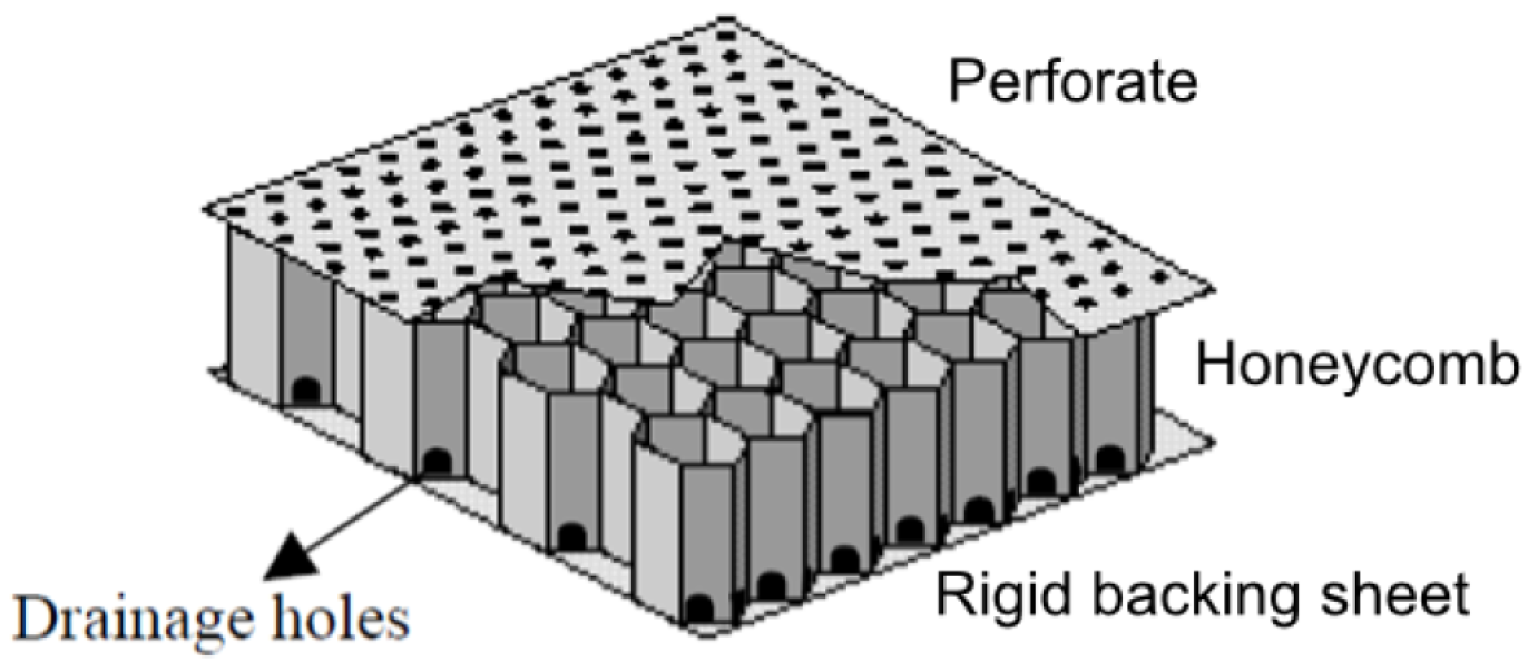
Figure 1. Schematic of the acoustic liner (adapted from [8]).
Aerospace 11 00717 g001
Figure 2. Reduced domain of the computational model (adapted from [8]).
Aerospace 11 00717 g002
Figure 3. Statistical convergence analysis of the GKDE for the conditional covariance matrix [ C H | W ( w ) ] of H , given W = w . Graph of n ar ( n ar ν + 1 ) 1 j = ν + 1 n ar [ C H | W ( w ar j ) ] 2 . Horizontal axis: n ar ν .
Aerospace 11 00717 g003
Figure 4. Conditional covariance matrices with the GKDE-based estimation of the conditional covariance of resistance (ad) and reactance (eh), given four different values of w .
Aerospace 11 00717 g004
Figure 5. Conditional covariance matrices with the statistical ANN-based metamodel estimation of the conditional covariance of resistance (ad) and reactance (eh), given four different values of w .
Aerospace 11 00717 g005
Figure 6. Random generations of frequency-sampled impedance using the statistical ANN-based metamodel. Conditional mean value (dashed blue line) and conditional confidence region (blue region) with a probability level P c = 98 % for the resistance (ad) and reactance (eh). The 10 thin black lines represent realizations of the frequency-sampled impedance generated by the statistical ANN-based metamodel for a given w . The horizontal axis represents the frequency in Hz.
Aerospace 11 00717 g006
Figure 7. Conditional mean values and conditional confidence region with a probability level P c = 98 % of the frequency-sampled impedance for the resistance (ad) and reactance (eh). The red dashed curve and the red zone represent the conditional mean values and conditional confidence intervals, respectively, estimated from [18] and the Silverman bandwidth fixed at s = 0.1186 for all the figures. The blue dashed curve and the blue zone represent the conditional expectation and conditional confidence intervals estimated using the statistical ANN-based metamodel of liner impedance, respectively. The horizontal axis represents the frequency in Hz.
Aerospace 11 00717 g007
Disclaimer/Publisher’s Note: The statements, opinions and data contained in all publications are solely those of the individual author(s) and contributor(s) and not of MDPI and/or the editor(s). MDPI and/or the editor(s) disclaim responsibility for any injury to people or property resulting from any ideas, methods, instructions or products referred to in the content.