Abstract
This paper presents a valley path planning algorithm based on the Hybrid A* algorithm. This algorithm is aimed at finding the valley path for aircraft considering dynamics constraints and terrain limitations. The preliminaries involve the establishment of a 3D workspace based on digital elevation map (DEM) data and addressing methods of valley detection. Following this comprehensive groundwork, the Hybrid A*-based algorithm, employed to determine the valley path within the 3D workspace while accommodating dynamic constraints and terrain limitations, is then introduced. In the experimental test, to validate the effectiveness of the algorithm proposed in this paper, we tested the performance of the proposed algorithm and other three baseline algorithms based on four optimization objectives in three workspaces. The simulated results indicate that the algorithm proposed in this paper can effectively find the valley path while considering dynamic constraints and terrain limitations.
1. Introduction
Valley path planning, a crucial facet of route optimization, emerges as a pivotal research area within robotics, autonomous vehicles, and geographic information systems (GISs). In the military field, valley path planning is of particular importance in terms of covert penetration and radar avoidance. By navigating along valleys, aircraft can exploit natural terrain features to enhance stealth capabilities, enabling effective avoidance of radar detection and other surveillance systems. In the realm of unmanned aerial vehicles (UAVs), the application of valley path planning extends to a myriad of scenarios, ensuring safe and efficient execution of tasks such as geological exploration, detection missions, search and rescue operations, environmental monitoring, resource exploration, and agricultural precision spraying. The utilization of valleys as preferred routes enhances the safety, precision, and success of these operations, showcasing the versatility and broad applicability of valley line path planning in the field of aerial systems.
In recent years, numerous researchers [1,2,3,4,5] have made in-depth exploration of similar studies. These investigations focus on enhancing path planning algorithms to meet the demands of complex terrains, with a specific emphasis on optimizing valley path planning. Researchers are dedicated to leveraging advanced computational methods and geographic information technologies to comprehensively and efficiently consider terrain features, providing more precise and viable solutions for path planning.
D. L. Page et al. [6,7] presented a tactical path planning algorithm for following ridges or valleys across a 3D terrain. The intent was to generate a path that enables an unmanned vehicle to surveil with maximum observability by traversing the ridges of a terrain or to operate with maximum covertness by navigating the valleys. However, the construction of triangle mesh cost huge time, resulting in poor algorithm timeliness. To give autonomous operation capability to unmanned aerial vehicles (UAVs), Isli et al. [8] presented an offline path planner which was based on evolutionary algorithms (EAs) and could calculate a curved path line with desired attributes in a 3D terrain. However, evolutionary algorithms can be computationally expensive, especially for problems with large search spaces or complex fitness landscapes. Jaillet et al. [9] presented a new method called transition-based RRT (T-RRT) for path planning problems in continuous cost spaces. Simulation results showed that the method could be applied to a large set of applications including terrain cost map motions or in planning low-cost motions for free-flying or articulated robots. However, the path obtained by T-RRT was not optimal and was full of twists and turns. Nikolos et al. [10] suggested an offline/online path planner for cooperating unmanned vehicles that took into account the mission objectives and constraints through an optimization procedure. However, the planned path contained significant turns and did not fully consider the dynamic constraints. To realize 3D space perception, Yuichiro et al. [11] proposed a GNG-DT-based 3D perception method by utilizing multiple topological structures for perceiving the 3D unknown terrain environment and a path planning method to the target point set in the unknown area. Experimental results of the proposed method used simulated terrain environments to verify the effectiveness of the proposed method. However, training neural networks requires a large amount of high-resolution data. To solve the problem that the surface of a planetary body is mostly covered with powdery soil and causes wheel slippage that will make the rover get stuck or tip over, Genya et al. [12] developed a path planning algorithm and a path evaluation method based on wheel-slip dynamics. In this approach, a path on rough terrain was first simply generated with a terrain-based criteria function. Examples of the proposed technique were demonstrated by discussing characteristics of the planned path and the slip motion profile of the rover to address the prediction errors of machine learning (ML) in evaluating the traversability of rovers on deformable terrain. However, the algorithm-generated path contained a large number of turns, resulting in a longer path length. Masafumi et al. [13] proposed a new path planning algorithm that explicitly accounts for such erroneous prediction. The algorithm gave us a multimodal slip distribution, accounting for heterogeneous terrains, and further allowed statistical risk assessment to be applied to derive risk-aware traversing costs for path planning. However, the article may not fully address the adaptation of the path planning approach to dynamic changes in the terrain. Lim et al. [14] presented a constrained valley detection algorithm. The intent was to find valleys on the map for path planning that enable a robot or a vehicle to move safely. The constraints to the valley are a desired width and a desired depth to ensure the space for movement when a vehicle passes through the valley. However, the algorithm just satisfies two-dimensional constraints. Xu et al. [15] presented a path planning approach for rotary unmanned aerial vehicles (R-UAVs) in a known static rough-terrain environment. This approach aims to find collision-free and feasible paths with minimum altitude, length, and angle variable rate. Experimental results under two different rough terrains from Guilin and Lanzhou in China demonstrated the capabilities of the proposed algorithm in finding Pareto optimal paths. Due to multiobjective optimization, the algorithm requires substantial computational power and has long calculation times. Ueli et al. [16] proposed a real-time optimization-based approach to terrain modeling and path planning in offroad and rough environments. Experiments with an unmanned ground vehicle in both structured and unstructured environments illustrated the applicability of the method. However, the article may not provide sufficient performance evaluations and comparative analyses with other existing methods, making it challenging for readers to assess the advantages and limitations of the proposed method. To address the problem of path planning for a rover in rugged terrain, Rekha et al. [17] proposed a new motion planning algorithm on rough terrain for a six-wheel rover with 10 DOF (degrees of freedom) by introducing a gradient function in the conventional potential field method. Simulation and experimental results showed the usefulness of the new method for generating paths in rough terrains. However, the proposed method may be tailored specifically for a six-wheel rover, limiting its applicability to other types of rovers or robotic systems operating in similar rough-terrain environments. Saranya et al. [18] presented a modified-approach D* path planning algorithm. Results with different test scenarios showed the effectiveness of the algorithm. However, the article might not thoroughly discuss the computational efficiency of the terrain-based D* algorithm, particularly in large-scale or complex terrains, which is essential for practical implementation. To tackle the problem of energy-efficient coverage path planning for exploring general surfaces by an autonomous vehicle, Wu et al. [19] developed an efficient algorithm which is used to generate paths on free-form 3D surfaces according to a special design pattern using a height-extremity-aware Fermat spiral. Physical experiments were conducted on different terrain surfaces to demonstrate the effectiveness of the approach. However, the paper might not thoroughly address dynamic energy constraints, such as varying energy consumption rates based on terrain types, or unexpected environmental factors, which are crucial for realistic energy-efficient path planning. Wu et al. [20] presented a geodesic-based planning and replanning algorithm as a new method for obstacle avoidance on a 3D terrain without using boundary following on the obstacle surface. A simulation demonstrated the practicality of the analytical geodesic replanning procedure for navigating a constant-speed-point robot on a 3D hill-like terrain. However, the paper might not thoroughly discuss the computational efficiency of the proposed approach, particularly in large-scale or complex 3D terrains.
The Hybrid A* algorithm is a cutting-edge path planning technique extensively utilized in robotics and autonomous vehicle navigation [21,22,23,24,25]. By blending discrete and continuous search algorithms, Hybrid A* can efficiently explore the configuration space to identify viable paths for vehicles maneuvering through intricate environments. Its ability to integrate vehicle dynamics and constraints ensures the generation of collision-free and feasible paths, while heuristic guidance enhances search efficiency, making it an invaluable tool for navigating complex terrains in applications such as autonomous driving and planetary exploration. The Hybrid A* algorithm offers several advantages, including efficiency by combining grid-based search with continuous motion planning for faster pathfinding, optimality in generating smoother paths that adhere to vehicle dynamics, robustness in adapting to dynamic environments for real-time applications, effective global planning for long-distance navigation through complex environments, scalability in managing large state spaces efficiently, and versatility across various vehicles and environments for broad usability.
Zheng et al. [26] proposed an AMCL-Hybrid A* method to enable robot navigation. The experimental results demonstrated the robot’s effective avoidance of both static and dynamic obstacles under this approach. Li et al. [24] introduced a new path planning method based on Hybrid A*. The method involves the initial construction of a local map using a prior road map, obstacle information, and contours of other AMRs. Subsequently, path planning is successfully executed in a limited manufacturing scenario using a variable-curvature Hybrid A* search. Saedi et al. [21] presented an innovative and computationally efficient approach that blends the well-known Hybrid A* search engine with visibility diagram planning to identify the shortest nonholonomic path in a hybrid (continuous-discrete) environment for valet parking. Ahmed et al. [25] proposed a hybrid approach that combines the modified APF algorithm’s global optimization capabilities with the real-time adaptability of the Hybrid A* path planning technique to overcome traditional APF local minimum issues. The results of various experiments demonstrate the effectiveness of the hybrid algorithm in different environments. The enhanced APF was shown to reach an optimal path to the goal 50% faster than A* and successfully navigated out of local minimums compared to traditional APF while also finding a shorter path than Hybrid A*. Sheng et al. [27] introduced a multistage Hybrid A* algorithm designed to address narrow passages formed by obstacles in cluttered environments. The algorithm conducts a 2D hybrid A* search to find a global route connecting the start and goal points and employs the Hybrid A* algorithm to find linking paths connecting adjacent subpaths. Simulation results indicated that the hierarchical trajectory planner operates significantly faster than prevalent methods when dealing with unstructured environments featuring narrow passages. To further enhance path safety and efficiency in autonomous parking systems, Meng et al. [28] proposed an improved Hybrid A* algorithm through safety-enhanced and efficiency-enhanced designs. Simulation experiments verified that the improved algorithm not only generates a much safer path, staying farther from obstacles, but also significantly improves searching efficiency in terms of time and space at a finite cost of preprocessing work that can be repeatedly utilized.
In this paper, our focus lies on the development of a valley path planning algorithm tailored for aircraft. The primary objective of this algorithm is to chart a flight path that closely aligns with the natural contours of the valley, all the while taking into account dynamic constraints, obstacle constraints, and the inherent terrain features. To establish a solid foundation, we begin by creating a workspace using real digital elevation model data and elucidating the concept of valleys along with the methodology for valley detection. Subsequently, we present the Hybrid A*-based algorithm, encompassing the workflow of the Hybrid A* algorithm, the formulation of heuristic search functions, the principles underpinning collision detection, and the theory of node expansion. This algorithm is designed to guide the aircraft along the valley line while mitigating obstacles to the greatest extent possible. Finally, we validate the efficacy of our algorithm by conducting simulations across three distinct scenarios and benchmarking against three different baseline algorithms to assess its performance.
This paper is organized as follows. In Section 2, we define the problem. In Section 3, preliminary works are presented. Then the workflow of the Hybrid A*-based algorithm and path connection methods are introduced in Section 4. In Section 5, a simulated test is proposed and results of optimal techniques proposed in this paper are presented. At last, some concluding remarks are made in Section 6.
2. Problem Definition
Let (t) = (x, y, z, , , ) ∈ = be the state of the aircraft dynamics model and ∈ be the input of the model. We can describe aircraft dynamics model by
Define as the workspace composed of DEM data. Let (, ) denote the mobile path starting from the start point and reaching the goal point . The path must satisfy that the elevation value of each path point is greater than the local terrain elevation , which means . In addition, the planned path must adhere to aircraft dynamics constraints, such as avoiding excessive turns and ensuring that the difference in altitude values between adjacent waypoints and is not too excessive, which means .
Define as the average deviation between the path point and the valley point. Define as the average elevation of . Define as the length of , and define as the cost time of the search algorithm. We are committed to finding a collision-free path while minimizing the average valley point deviation , average elevation , path length , and cost time :
where (, f(, )), (, f(, )), and (, f(, )), respectively, denote the average deviation, average elevation, and path length calculation model which will be introduced in Section 4.
3. Preliminaries
3.1. Workspace
In this paper, we construct the workspace using DEM data. DEM is a digital representation of ground surface topography or terrain. It provides a detailed and accurate depiction of elevation data for specific geographic areas, typically represented as a grid of regularly spaced points. DEM data are instrumental in various geospatial applications, including terrain analysis, watershed modeling, view shed analysis, and 3D visualization. By capturing elevation information, DEM data enable the visualization and analysis of terrain features, such as slopes, aspects, and contours, essential for a wide range of environmental, urban planning, and engineering purposes.
In our research, we selected three areas with prominent valley features as our workspace and downloaded the elevation data for these three areas from the U.S. Geological Survey website at www.usgs.gov (accessed on 4 February 2024). These three workspace are shown in Figure 1, Figure 2 and Figure 3.
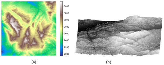
Figure 1.
Illustrative plot of workspace 1. (a) Two-dimensional plot of workspace 1. (b) Three-dimensional plot of workspace 1.
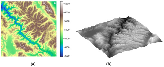
Figure 2.
Illustrative plot of workspace 2. (a) Two-dimensional plot of workspace 2. (b) Three-dimensional plot of workspace 2.
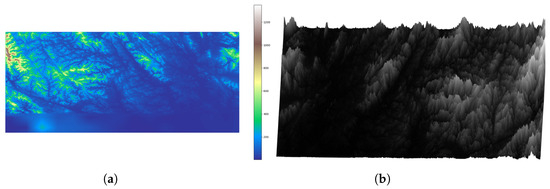
Figure 3.
Illustrative plot of workspace 3. (a) Two-dimensional plot of workspace 3. (b) Three-dimensional plot of workspace 3.
3.2. Valley Description
A valley can be defined as the local minimum of the continuous function that represents the topographic profile of the landscape. In mathematical terms, a valley can be expressed as the point on the function where the first derivative is zero and the second derivative is positive, indicating the lowest point in the surrounding area (Figure 4 shows illustrative plot of valley and ridge points). Referring to the literature [6,7], we denote the maximum and minimum principal curvatures as and ( ≥ ) of a specific area of digital elevation maps. We define and as unit vectors of and . We can further define the derivatives of the principal curvatures along their associated directions as
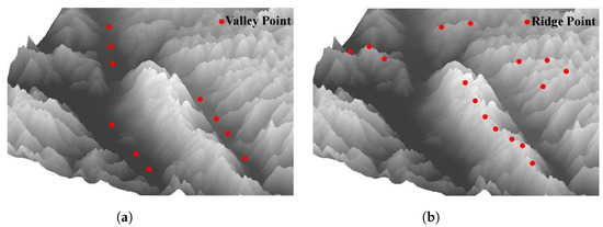
Figure 4.
Illustrative plot of valley and ridge points. (a) Illustrative plot of valley points. (b) Illustrative plot of ridge points.
Furthermore, the description of the valley’s characteristics is as follows:
3.3. Valley Point Detection
In this section, we conducted valley detection by determining whether there is any obstruction on either side of a specific point q. The core idea is as follows: for a specific point , is the height of q. Assume is the velocity direction of q. Assume and are two points on the left and right sides of point q, perpendicular to the velocity direction of (shown in Figure 5).
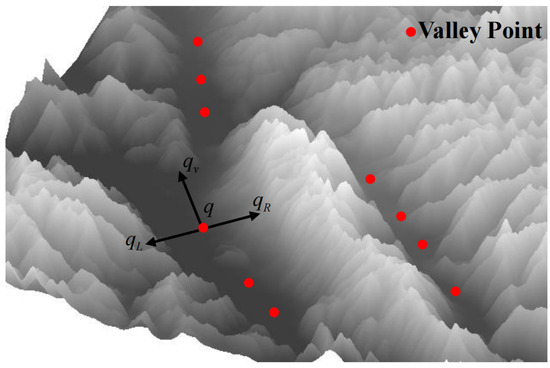
Figure 5.
Illustrative plot of valley detection methods.
Suppose and are elevation data of and , and and are the height of and . Equation (9) describes that both sides are obstructed.
4. Hybrid A*-Based Valley Detection Algorithm
4.1. Workflow of Hybrid A* Algorithm
The Hybrid A* algorithm is a cutting-edge path planning technique extensively utilized in robotics and autonomous vehicle navigation. By blending discrete and continuous search algorithms, Hybrid A* can efficiently explore the configuration space to identify viable paths for vehicles maneuvering through intricate environments. Its ability to integrate vehicle dynamics and constraints ensures the generation of collision-free and feasible paths, while heuristic guidance enhances search efficiency, making it an invaluable tool for navigating complex terrains in applications such as autonomous driving and planetary exploration.
The pseudocode for the Hybrid A* algorithm, as presented in Algorithm 1, begins with initializing the start point (), goal point (), open list (), and closed list () (line 1). At the start of each iteration, find node with minimum cost in the open list as the current node (line 3). Then, the algorithm examines whether the distance between and is less than an expanding step or if can directly connect to the goal without encountering any collisions (lines 4–6). If these conditions are not met, expand the node to obtain a set of nodes U within a certain search range (line 7). For each node in the node set U, first calculate cost using cost functions and store in the (line 12). If is already in the closed list , continue (lines 13–15); if is already in the open list , check whether the cost of new is larger than that of original . If this is the case, replace original with new (lines 16–20). Upon completion of the entire search process, a feasible path can be derived by tracing back from to and obtaining valley path (line 23).
| Algorithm 1: Hybrid A* algorithm |
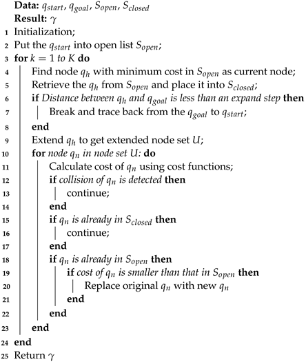 |
In the Hybrid A* algorithm, the handling of the open list and closed list is a crucial part of the algorithm. This includes several key components for managing the open list and closed list :
- Initialize and create empty open and closed lists and ;
- Place the root node into the open list ;
- Retrieve the node with the minimum cost from the open list ;
- Place node into the closed list ;
- Based on , generate node set U, and place from U into the open list if satisfies no collision, is not in the closed list , and has a smaller cost.
4.2. Collision Detection
Given the irregular and rugged terrain in the workspace, as opposed to being flat, planned trajectories run the risk of intersecting with the ground or encountering scenarios resembling “terrain piercing.” Hence, it becomes imperative to implement collision detection.
The methodology for collision detection based on DEM data is as follows: for the corresponding two adjacent waypoints and , an intermediate set of waypoints U is generated through linear interpolation. If the altitude values of these waypoints exceed the sum of the terrain elevation and the safety margin , there is no risk of collision with the terrain. Conversely, if this condition is not met, a collision is imminent.
4.3. Cost Functions
The Hybrid A* algorithm utilizes cost functions to efficiently navigate through complex environments. These cost functions include the actual cost and heuristic cost .
The actual cost, often denoted as , is a fundamental metric used to evaluate the efficiency and feasibility of potential paths. It represents the cumulative cost incurred from the starting point to the current node along the explored path. This cost incorporates various factors, including the distance traveled, any penalties or constraints imposed by the environment, and considerations of vehicle dynamics. By analyzing the actual cost, the Hybrid A* algorithm optimizes path planning by prioritizing paths with lower accumulated costs, leading to smoother and more efficient trajectories for vehicles navigating complex environments. In our study, actual cost represents the path cost from the starting point to the current node, accounting for the distance traveled.
Heuristic cost plays a crucial role in guiding the search process towards the most promising areas of the search space, thereby improving the efficiency of the search algorithm. The heuristic cost is typically designed by considering factors such as distance to the goal, terrain difficulty, and any other relevant constraints. It often involves estimating the remaining cost from the current state to the goal state. This estimation helps guide the search towards the goal efficiently. The specific design of the heuristic cost can vary based on the problem domain and requirements.
In our study, heuristic cost consists of five components, which are valley point deviation cost , average elevation cost , path length cost , height cost , and valley cost , and with their weight coefficients, , , , , and , respectively.
Our heuristic search function is designed as follows: first, we account for the deviation of valley points, as outlined in Section 3.3, by implementing a method to detect them. This allows us to plan paths that closely adhere to the valley lines. We then incorporate the deviation of valley points into the heuristic cost (valley point deviation cost , which will be introduced in Section 4.3.1), aiming for the algorithm to minimize this deviation along the newly obtained path points during the search. Next, we assess the average elevation value, considering that valley points indicate local elevation minima and prioritizing paths aligned with the valley lines. The average elevation value becomes a component of the heuristic (average elevation cost , which will be introduced in Section 4.3.2). Following this, we evaluate the path length from the current point to the target point (path length cost , which will be introduced in Section 4.3.3), drawing inspiration from the Hybrid A* algorithm to expedite the target location process. Subsequently, we factor in the height cost, integrating it into the heuristic cost to align paths with the valley lines (height cost , which will be introduced in Section 4.3.4). Lastly, we address the valley cost (, which will be introduced in Section 4.3.5), assigning a negative value whenever a newly expanded node is identified as a valley point. This encourages the algorithm to explore paths closely following the valley points. In conclusion, the primary objective of this heuristic design is to optimize path selection along the valley lines while meeting the speed requirements of the search process.
By combining actual cost and heuristic cost functions, the Hybrid A* algorithm can effectively generate optimal paths while accounting for both kinematic and dynamic constraints, making it well suited for autonomous navigation in real-world scenarios.
4.3.1. Valley Point Deviation
Assuming there are n points along the route, along with m valley points. Let represent the distance between the point on the route and the valley point, then the distance between the route point and the nearest valley point can be represented as
The valley deviation of the flight path can be obtained by accumulating the distance between each route point and the nearest valley point.
The average valley point deviation is obtained by dividing by the total number of points n along the route.
4.3.2. Average Elevation Cost
Assuming there are n points along the flight route with respective elevation values , , …, , the average elevation value can be calculated using the following equation:
4.3.3. Path Length Cost
Supposing that there are n points along the flight route and and are two adjacent points, then the distance between the two points is
The path length from the initial point to the current point is calculated as follows:
4.3.4. Height Cost
Assuming is the current waypoint, is the elevation of . is a potential next path point, and is the elevation of . Then height cost can be calculated as follows:
In Equation (18), is the height weighting coefficient.
4.3.5. Valley Cost
Assuming is the current waypoint and is a valley point (the method of determining whether q is a valley point was introduced in Section 2), assign a negative path cost to .
4.4. Node Expansion
4.4.1. Minimum Turning Radius
The turning radius of an aircraft refers to the radius of the circle it traces while executing a turn. It is a crucial parameter in aviation, determining the maneuverability and spatial requirements of the aircraft during flight. The turning radius of aircraft R can be calculated as follows:
In Equation (19), g, V, and represent gravitational acceleration, the true airspeed, and the bank angle of the aircraft, respectively.
The minimum turning radius of an aircraft refers to the smallest radius of a circle within which the aircraft can complete a turn while maintaining control and stability. It is a critical parameter in aviation, determining the minimum space required for maneuvering and navigating through airspace, especially in confined or congested areas such as airports or during aerial combat. For our own aircraft dynamics model, the minimum turning radius is 120 m.
4.4.2. Angle Discretization
In this algorithm, we conduct a search in three-dimensional space by discretizing the heading angle in the horizontal plane and the pitch angle in the vertical plane.
Node expansion on a two-dimensional plane involves breaking down the search space into discrete angular increments of heading angles. Assuming the current heading angle is , the maximum exploration angle in the horizontal plane is , and the discretized angle is , then the maximum exploration heading angles on both sides are calculated as follows:
Therefore, we can obtain the following set of heading angle searches on the horizontal plane:
Based on the same idea, we can obtain the pitch angle search set in the vertical plane:
In Equation (22), and represent the maximum pitch angles for the upper and lower sides, respectively.
4.4.3. Node Generation
Based on the minimum turning radius and angle discretization, we can discretely search for new nodes in three-dimensional space, assuming the current node is (, , , ), where , , , and represent the current three-dimensional coordinates and heading angle of the aircraft. Assuming the search angles in the horizontal and vertical planes are and , respectively, the calculation for the new node based on this horizontal heading angle and pitch angle is as follows:
Based on Equation (23), we can obtain the expanded node set U. Then, using the cost function introduced in Section 4.2 and Section 4.3, we calculate the cost of each collision-free node and select the node with the highest cost as the next time-step’s expansion node .
4.5. Hybrid A*-Based Valley Path Planning Algorithm
In this section, we introduce the Hybrid A*-based valley path planning algorithm, which is utilized to search for the valley path. This algorithm incorporates the previously introduced cost function and collision detection algorithm.
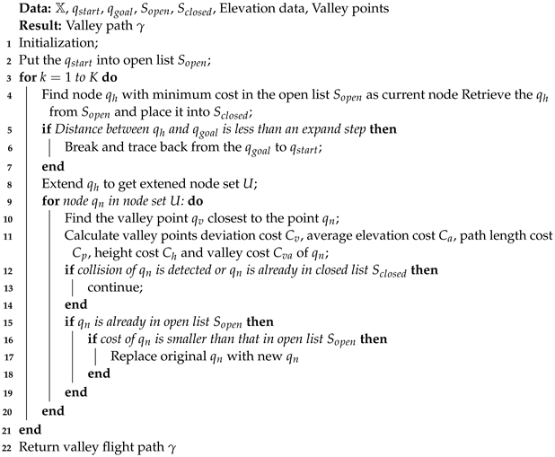
The pseudocode for the Hybrid A*-based valley path planning algorithm, as presented in Algorithm 2, begins with detecting and saving valley points of selected elevation data (line 1). Then initialize start point (), goal point (), , and closed list (line 2). At the start of each iteration, find node with minimum cost in the open list as the current node (line 3). Expand the node to obtain a set of nodes U within a certain search range (line 7). For each node in the node set U, calculate valley cost , average elevation cost , path length cost , height cost , and valley cost , and store in the (lines 8–10). If there is any collision in , continue (lines 11–13), or if is already in the closed list , continue (lines 11–13); if is already in open list , check whether the cost of new is larger than that of original . If this is the case, replace original with new (lines 14–18). Upon completion of the entire search process, a valley path can be derived by tracing back from to (line 21).
| Algorithm 2: Hybrid A*-based path planning algorithm |
 |
5. Experimental Test
In this section, we conducted a literature review and selected three representative algorithms: Dijkstra, artificial potential field (APF), and transition-based RRT (T-RRT) [6,9,29]. Based on the construction of three workspaces (workspace 1, workspace 2, and workspace 3, which were introduced in Section 3) and four optimization objectives, average elevation, path length, valley point deviation, and time cost, we carried out performance evaluations of these four algorithms (the proposed Hybrid-A* based algorithm and the other three baseline algorithms).
Dijkstra’s algorithm is a fundamental algorithm for finding the shortest path between nodes in a graph. This algorithm is widely used in various applications, such as network routing protocols and transportation systems. The key idea behind Dijkstra’s algorithm is to iteratively explore the nodes of the graph starting from a chosen source node, updating the shortest distance to each node as it traverses the graph. By keeping track of the shortest distances and the path that leads to each node, Dijkstra’s algorithm efficiently determines the shortest path from the source node to all other nodes in the graph. The algorithm is known for its simplicity and efficiency, making it a popular choice for solving shortest-path problems in computer science and related fields.
The APF algorithm is a popular method used in robotics and artificial intelligence for path planning and navigation tasks. APF mimics the behavior of objects moving in a physical field influenced by attractive and repulsive forces. In APF, the robot or agent is represented as a point in a potential field, where attractive forces pull it towards the goal while repulsive forces push it away from obstacles. By summing these forces, the robot can navigate through complex environments while avoiding collisions with obstacles. APF is known for its simplicity and effectiveness in real-time applications, making it a valuable tool for autonomous navigation and robotics.
T-RRT is proposed for path planning on configuration-space cost maps. The algorithm considers a user-given cost function defined over the configuration space as an additional input to the standard path planning problem, and it produces solution paths that are not only feasible (e.g., collision free) but also have good quality with respect to the input cost map.
5.1. Valley Point Detection
Using the previously described valley point detection method, we identified the valley points of these three workspaces and saved them as bias waypoints for the subsequent Hybrid A*-based algorithm search. Figure 6, Figure 7 and Figure 8 display the results of our valley point detection. In these figures, the red points represent the detected valley points.
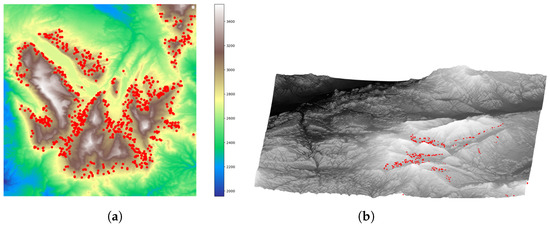
Figure 6.
Illustrative plot of valley detection on workspace 1. (a) Illustrative plot of workspace 1. (b) Illustrative plot of workspace 1.
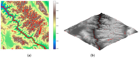
Figure 7.
Illustrative plot of valley detection on workspace 2. (a) Illustrative plot of workspace 2. (b) Illustrative plot of workspace 2.
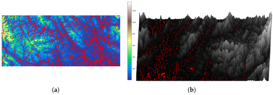
Figure 8.
Illustrative plot of valley detection on workspace 3. (a) Illustrative plot of workspace 3. (b) Illustrative plot of workspace 3.
5.2. Simulation Results
In this section, we showcase the simulated results of the algorithm proposed in this paper alongside three algorithms, T-RRT, APF, and Dijkstra [6,9,29], which are frequently referenced in the literature.
In our experiment, we adopted the Windows 10 operating system. The programming language we chose was Python, specifically Python 3.7. The processor used was the 10th Gen Intel Core i9-10805K @ 3.60-GHz Deca-core processor (Intel, Santa Clara, CA, USA), renowned for its powerful computing power and multicore performance suitable for deep learning tasks. We used 16-GB RAM. For graphics processing, we employed the NVIDIA GeForce RTX 3070 (NVIDIA, Santa Clara, CA, USA), enabling accelerated training of deep learning models and providing high-performance parallel computing capabilities.
5.2.1. Workspace 1
In workspace 1, we selected two sets of different start–end point pairs and conducted tests on these two sets of start–end point pairs. Figure 9 and Figure 10 show the plots of search results. Table 1 and Table 2 present path planning results for start–end set 1 and 2 in workspace 1 of our proposed algorithm and the other three algorithms.
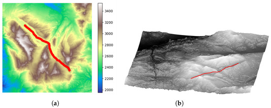
Figure 9.
Path planning results of proposed algorithm in workspace 1 (start–end set 1). (a) The 2D path planning results for workspace 1. (b) The 3D path planning results for workspace 1.
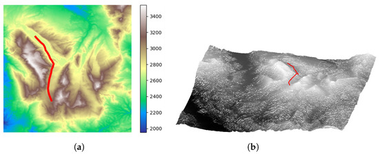
Figure 10.
Path planning results of proposed algorithm in workspace 1 (start–end set 2). (a) The 2D path planning results for workspace 1. (b) The 3D path planning results for workspace 1.

Table 1.
Path planning results for start–end set 1 in workspace 1.

Table 2.
Path planning results for start–end set 2 in workspace 1.
Figure 9a and Figure 10a are the two-dimensional elevation maps of workspace 1, and Figure 9b and Figure 10b are the three-dimensional terrain maps of workspace 1. The red curve represents the planned path. It can be observed that for different start–end point pairs, the algorithm proposed in this paper plans paths that effectively follow the valley lines.
In Table 1 and Table 2, we can see that compared to the other three baseline algorithms, our proposed algorithm shows outstanding performance in terms of average elevation, valley point deviation, and algorithm execution time. It is worth mentioning that due to the need to follow the valley lines, the paths planned by the algorithm proposed in this paper will be longer than those of the other three algorithms.
5.2.2. Workspace 2
Workspace 2 features rich valley terrain characteristics. In workspace 2, we selected three sets of different start–end point pairs and conducted tests on these three sets of start–end point pairs. Figure 11, Figure 12 and Figure 13 display the search results. In these figures, the red curve represents the planned path. Table 3, Table 4 and Table 5 present the path planning results for these three sets of start–end point pairs in workspace 2 of our proposed algorithm and the other three algorithms.
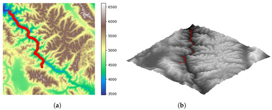
Figure 11.
Path planning results of proposed algorithm in workspace 2 (start–end set 1). (a) The 2D path planning results for workspace 2. (b) The 3D path planning results for workspace 2.
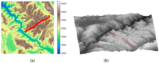
Figure 12.
Path planning results of proposed algorithm in workspace 2 (start–end set 2). (a) The 2D path planning results for workspace 2. (b) The 3D path planning results for workspace 2.
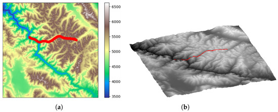
Figure 13.
Path planning results of proposed algorithm in workspace 2 (start–end set 3). (a) The 2D path planning results for workspace 2. (b) The 3D path planning results for workspace 2.

Table 3.
Path planning results for start–end set 1 in workspace 2.

Table 4.
Path planning results for start–end set 2 in workspace 2.

Table 5.
Path planning results for start–end set 3 in workspace 2.
5.2.3. Workspace 3
Workspace 3 has lower average elevation values, making the terrain relatively flat compared to workspace 1 and workspace 2. In workspace 3, we selected two sets of different start–end point pairs and conducted tests on these two sets of start–end point pairs. Figure 14 and Figure 15 display the search results. In these figures, the red curve represents the planned path. Table 6 and Table 7 present the path planning results of our proposed algorithm and the other three algorithms.
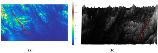
Figure 14.
Path planning results of proposed algorithm in workspace 3 (start–end set 1). (a) The 2D path planning results for workspace 3. (b) The 3D path planning results for workspace 3.

Figure 15.
Path planning results of proposed algorithm in workspace 3 (start–end set 2). (a) The 2D path planning results for workspace 3. (b) The 3D path planning results for workspace 3.

Table 6.
Path planning results for start–end set 1 in workspace 3.

Table 7.
Path planning results for start–end set 2 in workspace 3.
5.3. Discussion
From Figure 9, Figure 10, Figure 11, Figure 12, Figure 13, Figure 14 and Figure 15 and Table 1, Table 2, Table 3, Table 4, Table 5, Table 6 and Table 7, it can be seen that for three different workspaces and various start–end point pairs, compared to the other three algorithms, the algorithm proposed in this paper achieved better results in terms of valley point deviation, average elevation, and algorithm execution time. This means that the routes planned by our algorithm can better follow the valley lines. However, valley lines are often winding and meandering, so following the valley lines results in longer path lengths. This explains why the path length results of our algorithm are greater than the other three algorithms.
Compared to the Dijkstra algorithm, our algorithm takes into account the dynamic constraints of aircraft, which results in paths that are more realistic and feasible. By considering the aerodynamic limitations and capabilities of aircraft, our algorithm generates trajectories that are not only efficient but also adhere closely to real-world conditions.
The APF algorithm achieves exploration of targets and avoidance of obstacles by establishing attractive and repulsive potential functions, but its drawback is the tendency to get stuck in local minima. Our algorithm effectively avoids local minima by considering actual dynamic constraints and designing a cost function that includes subitems such as deviations in valley points. This enables fast and efficient exploration of valley line paths.
The TRRT algorithm is an improvement upon the RRT algorithm, inheriting its advantages of speed and efficiency. However, the paths it plans often contain many zigzags and lack smoothness, necessitating further smoothing using path smoothing algorithms. In contrast, our algorithm inherits the advantages of the Hybrid A* algorithm, resulting in smoother paths.
In general, our algorithm incorporates a cost function that takes into account deviations in valley points, differences in elevation values, and path length, which are not present in the other three algorithms. The design of this cost function enabled us to efficiently and swiftly plan routes along valley lines.
5.4. Summary
In this section, we tested the algorithm proposed in this paper and three baseline algorithms based on three workspaces and four optimization objectives, confirming the effectiveness of the algorithm proposed in this paper. The simulation results indicate that the algorithm proposed in this paper is able to rapidly plan valley paths while considering terrain constraints.
6. Conclusions
In this paper, a Hybrid A*-based valley path planning algorithm was presented. This study first introduced the foundational work, including workspace construction and valley point detection methods. Subsequently, we introduced the valley line path planning method based on Hybrid A*, focusing on the basic workflow of Hybrid A*, collision detection algorithms, the design of the cost function, and the theory of node expansion. In experimental tests, we evaluated the algorithm proposed in this paper along with three baseline algorithms across three different workspaces and four optimization objectives. Our findings confirmed the effectiveness of the proposed algorithm. The simulation results demonstrated that our algorithm can efficiently plan valley paths by taking terrain constraints into account.
Author Contributions
Conceptualization, T.X.; Software, T.X. and Y.C.; Resources, J.A.; Data curation, T.X.; Writing—original draft, T.X.; Writing—review & editing, Y.Z. and Y.D. All authors have read and agreed to the published version of the manuscript.
Funding
This research was funded by Shanghai Natural Fund grant number 22ZR1404500, Shanghai Pujiang Talent Program grant number 22PJ1413800 and the Fundamental Research Funds for the Central Universities number 22120240180.
Data Availability Statement
The data presented in this study are available on request from the corresponding author.
Conflicts of Interest
I hereby declare that there are no conflicts of interest associated with this work and the funders had no role in the design of the study; in the collection, analyses, or interpretation of data; in the writing of the manuscript; or in the decision to publish the results.
References
- Hu, Y.; Yang, S.X. A knowledge based genetic algorithm for path planning of a mobile robot. In Proceedings of the IEEE International Conference on Robotics and Automation, 2004, ICRA’04, New Orleans, LA, USA, 26 April–1 May 2004; Volume 5, pp. 4350–4355. [Google Scholar]
- Guo, T.Y.; Qu, D.-K.; Dong, Z.-L. Research of path planning for polishing robot based on improved genetic algorithm. In Proceedings of the 2004 IEEE International Conference on Robotics and Biomimetics, Shenyang, China, 22–26 August 2004; pp. 334–338. [Google Scholar]
- Ettlin, A.; Bleuler, H. Rough-terrain robot motion planning based on obstacleness. In Proceedings of the 2006 9th International Conference on Control, Automation, Robotics and Vision, Singapore, 5–8 December 2006; pp. 1–6. [Google Scholar]
- Ettlin, A.; Bleuler, H. Randomised rough-terrain robot motion planning. In Proceedings of the 2006 IEEE/RSJ International Conference on Intelligent Robots and Systems, Beijing, China, 9–13 October 2006; pp. 5798–5803. [Google Scholar]
- Ohtake, Y.; Belyaev, A.; Seidel, H.P. Ridge-valley lines on meshes via implicit surface fitting. In ACM SIGGRAPH 2004 Papers; ACM: New York, NY, USA, 2004; pp. 609–612. [Google Scholar]
- Page, D.L.; Koschan, A.F.; Abidi, M.A.; Overholt, J.L. Ridge-valley path planning for 3D terrains. In Proceedings of the 2006 IEEE International Conference on Robotics and Automation, ICRA, Orlando, FL, USA, 15–19 May 2006; pp. 119–124. [Google Scholar]
- Brecher, A.; Noronha, V.; Herold, M. UAV2003-A Roadmap for Deploying Unmanned Aerial Vehicles (UAVs) in Transportation. In Proceedings of the Volpe Center and NCRST Infrastructure Specialist Workshop, Santa Barbara, CA, USA, 2 December 2003. [Google Scholar]
- Hasircioglu, I.; Topcuoglu, H.R.; Ermis, M. 3-D path planning for the navigation of unmanned aerial vehicles by using evolutionary algorithms. In Proceedings of the 10th Annual Conference on Genetic and Evolutionary Computation, Atlanta, GA, USA, 12–16 July 2008; pp. 1499–1506. [Google Scholar]
- Jaillet, L.; Cortés, J.; Siméon, T. Sampling-based path planning on configuration-space costmaps. IEEE Trans. Robot. 2010, 26, 635–646. [Google Scholar] [CrossRef]
- Nikolos, I.K.; Tsourvelouds, N.C. Path planning for cooperating unmanned vehicles over 3-D terrain. In Informatics in Control, Automation and Robotics: Selected Papers from the International Conference on Informatics in Control, Automation and Robotics 2007; Springer: Berlin/Heidelberg, Germany, 2009; pp. 153–168. [Google Scholar]
- Torres, M.; Pelta, D.A.; Verdegay, J.L.; Torres, J.C. Coverage path planning with unmanned aerial vehicles for 3D terrain reconstruction. Expert Syst. Appl. 2016, 55, 441–451. [Google Scholar] [CrossRef]
- Ishigami, G.; Nagatani, K.; Yoshida, K. Path planning for planetary exploration rovers and its evaluation based on wheel slip dynamics. In Proceedings of the 2007 IEEE International Conference on Robotics and Automation, Rome, Italy, 10–14 April 2007; pp. 2361–2366. [Google Scholar]
- Endo, M.; Taniai, T.; Yonetani, R.; Ishigami, G. Risk-aware Path Planning via Probabilistic Fusion of Traversability Prediction for Planetary Rovers on Heterogeneous Terrains. arXiv 2023, arXiv:2303.01169. [Google Scholar]
- Lim, I.G.; Kim, J.S.; Lee, C.H. A Valley Detection for Path Planning. Int. J. Comput. Inf. Eng. 2009, 3, 2186–2189. [Google Scholar]
- Zhen, X.; Enze, Z.; Qingwei, C. Rotary unmanned aerial vehicles path planning in rough terrain based on multi-objective particle swarm optimization. J. Syst. Eng. Electron. 2020, 31, 130–141. [Google Scholar]
- Graf, U.; Borges, P.; Hernández, E.; Siegwart, R.; Dubé, R. Optimization-based terrain analysis and path planning in unstructured environments. In Proceedings of the 2019 International Conference on Robotics and Automation (ICRA), Montreal, QC, Canada, 20–24 May 2019; pp. 5614–5620. [Google Scholar]
- Raja, R.; Dutta, A.; Venkatesh, K.S. New potential field method for rough terrain path planning using genetic algorithm for a 6-wheel rover. Robot. Auton. Syst. 2015, 72, 295–306. [Google Scholar] [CrossRef]
- Saranya, C.; Unnikrishnan, M.; Ali, S.A.; Sheela, D.; Lalithambika, V. Terrain based D* algorithm for path planning. IFAC-Pap. Online 2016, 49, 178–182. [Google Scholar] [CrossRef]
- Wu, C.; Dai, C.; Gong, X.; Liu, Y.J.; Wang, J.; Gu, X.D.; Wang, C.C. Energy-efficient coverage path planning for general terrain surfaces. IEEE Robot. Autom. Lett. 2019, 4, 2584–2591. [Google Scholar] [CrossRef]
- Wu, K.L.; Ho, T.J.; Huang, S.A.; Lin, K.H.; Lin, Y.C.; Liu, J.S. Path planning and replanning for mobile robot navigation on 3D terrain: An approach based on geodesic. Math. Probl. Eng. 2016, 2016. [Google Scholar] [CrossRef]
- Sedighi, S.; Nguyen, D.V.; Kuhnert, K.D. Guided hybrid A-star path planning algorithm for valet parking applications. In Proceedings of the 2019 5th International Conference on Control, Automation and Robotics (ICCAR), Beijing, China, 19–22 April 2019; pp. 570–575. [Google Scholar]
- Dang, C.V.; Ahn, H.; Lee, D.S.; Lee, S.C. Improved analytic expansions in hybrid a-star path planning for non-holonomic robots. Appl. Sci. 2022, 12, 5999. [Google Scholar] [CrossRef]
- Cao, Z.; Wang, H.; Zhang, X.; Du, Y.; Zhang, D. Path Planning of Coastal Ships Based on Improved Hybrid A-Star. In Proceedings of the International Conference on Algorithms and Architectures for Parallel Processing, Tianjin, China, 20–22 October 2023; pp. 398–417. [Google Scholar]
- Li, C.; Yu, D.; Lu, W.; Li, M. Variable-curvature hybrid a-star search for amr path planning in limited space. In Proceedings of the 2021 3rd International Symposium on Robotics & Intelligent Manufacturing Technology (ISRIMT), Changzhou, China, 24–26 September 2021; pp. 61–65. [Google Scholar]
- Abdel-Rahman, A.S.; Zahran, S.; Elnaghi, B.E.; Nafea, S. Enhanced Hybrid Path Planning Algorithm Based on Apf and A-Star. Int. Arch. Photogramm. Remote. Sens. Spat. Inf. Sci. 2023, 48, 867–873. [Google Scholar] [CrossRef]
- Zheng, H.; Dai, M.; Zhang, Z.; Xia, Z.; Zhang, G.; Jia, F. The Navigation Based on Hybrid A Star and TEB Algorithm Implemented in Obstacles Avoidance. In Proceedings of the 2023 29th International Conference on Mechatronics and Machine Vision in Practice (M2VIP), Queenstown, New Zealand, 21–24 November 2023; pp. 1–6. [Google Scholar]
- Sheng, W.; Li, B.; Zhong, X. Autonomous parking trajectory planning with tiny passages: A combination of multistage hybrid A-star algorithm and numerical optimal control. IEEE Access 2021, 9, 102801–102810. [Google Scholar] [CrossRef]
- Meng, T.; Yang, T.; Huang, J.; Jin, W.; Zhang, W.; Jia, Y.; Wan, K.; Xiao, G.; Yang, D.; Zhong, Z. Improved Hybrid A-Star Algorithm for Path Planning in Autonomous Parking System Based on Multi-Stage Dynamic Optimization. Int. J. Automot. Technol. 2023, 24, 459–468. [Google Scholar] [CrossRef]
- Toda, Y.; Ozasa, K.; Matsuno, T. Growing neural gas based navigation system in unknown terrain environment for an autonomous mobile robot. Artif. Life Robot. 2023, 28, 76–88. [Google Scholar] [CrossRef]
Disclaimer/Publisher’s Note: The statements, opinions and data contained in all publications are solely those of the individual author(s) and contributor(s) and not of MDPI and/or the editor(s). MDPI and/or the editor(s) disclaim responsibility for any injury to people or property resulting from any ideas, methods, instructions or products referred to in the content. |
© 2024 by the authors. Licensee MDPI, Basel, Switzerland. This article is an open access article distributed under the terms and conditions of the Creative Commons Attribution (CC BY) license (https://creativecommons.org/licenses/by/4.0/).