Aircraft Wake Evolution Prediction Based on Parallel Hybrid Neural Network Model

Abstract

To overcome the time-consuming drawbacks of Computational Fluid Dynamics (CFD) numerical simulations, this paper proposes a hybrid model named PA-TLA (parallel architecture combining a TCN, LSTM, and an attention mechanism) based on the concept of intelligent aerodynamics and a parallel architecture. This model utilizes CFD data to drive efficient predictions of aircraft wake evolution at different initial altitudes during the approach phase. Initially, CFD simulations of continuous initial altitudes during the approach phase are used to generate aircraft wake evolution data, which are then validated against real-world LIDAR data to verify their reliability. The PA-TLA model is designed based on a parallel architecture, combining Long Short-Term Memory (LSTM) networks, Temporal Convolutional Networks (TCNs), and a tensor concatenation module based on the attention mechanism, which ensures computational efficiency while fully leveraging the advantages of each component in a parallel processing framework. The study results show that the PA-TLA model outperforms both the LSTM and TCN models in predicting the three characteristic parameters of aircraft wake: vorticity, circulation, and Q-criterion. Compared to the serially structured TCN-LSTM, PA-TLA achieves an average reduction in mean squared error (MSE) of 6.80%, in mean absolute error (MAE) of 7.70%, and in root mean square error (RMSE) of 4.47%, with an average increase in the coefficient of determination (R²) of 0.36% and a 35% improvement in prediction efficiency. Lastly, this study combines numerical simulations and the PA-TLA deep learning architecture to analyze the near-ground wake vortex evolution. The results indicate that the ground effect increases air resistance and turbulence as vortices approach the ground, thereby slowing the decay rate of the wake vortex strength at lower altitudes. The ground effect also accelerates the dissipation and movement of vortex centers, causing more pronounced changes in vortex spacing at lower altitudes. Additionally, the vortex center height at lower altitudes initially decreases and then increases, unlike the continuous decrease observed at higher altitudes.

1. Introduction

Aircraft wake turbulence is a byproduct of lift generation, characterized by its long duration, wide distribution, and high intensity. When an aircraft enters the wake region of a leading aircraft, the intense vortical structures induce rolling torques, causing the trailing aircraft to experience bumps, rolls, and changes in flight status. According to the Federal Aviation Administration (FAA), 78% of wake encounters from 1983 to 2000 occurred below 200 feet (61 m) [1]. During the approach phase, aircraft density increases along the glide path, and influenced by the ground effect, the wake may stall or rebound near the ground [2]; hence, the evolution of wake vortices varies at different heights during this phase. Wake separation also limits the number of flights that can take off and land at an airport per unit of time, significantly impacting airport capacity.

In the early 1970s, the International Civil Aviation Organization (ICAO) established standards for aircraft wake separation, which proved overly conservative due to a lack of consideration for meteorological factors and specific scenarios. To establish reasonable standards for the spacing of aircraft during approach and departure, and to effectively enhance airport capacity and air traffic operational efficiency, numerous scholars have begun systematic studies on aircraft wake, exploring its physical mechanisms. Traditional wake monitoring and prediction technologies include Computational Fluid Dynamics (CFD) simulations, wind tunnel and water tunnel experiments, and field radar detection. CFD simulations, in particular, simulate the characteristics and evolution of aircraft wake near the ground across various environments. Under clear sky conditions, classical numerical simulation techniques primarily involve Large Eddy Simulation (LES) methods and Reynolds-Averaged Navier–Stokes approaches. Holzäpfel and others [3,4] used aircraft wake velocity models as initial conditions for numerical simulations, significantly enhancing computational efficiency and accuracy. In terms of wake velocity models, research institutions in Europe and America, including the German Aerospace Center (DLR), Office National d’Études et de Recherches Aérospatiales (ONERA), and the National Aeronautics and Space Administration (NASA), have combined theoretical analysis, numerical simulation, and extensive experimental measurements to obtain the tangential velocity distribution of aircraft wake on cross-sections [5], with representative models including the Lamb–Oseen, Hallock–Burnham, Proctor, and Winckelmans models.

During the approach phase, the initial altitude of wake evolution varies, and wake vortices can be classified as either Out of Ground Effect (OGE) or In Ground Effect (IGE). Crow first analyzed the linear stability of vortex pairs in the OGE region [6]. He discovered that under certain disturbances, vortex pairs would incline about 45 degrees into a symmetric fixed plane and form sinusoidal shapes. Subsequently, the vortex pairs connect at their closest points, leading to the formation of a helical structure and the destruction of wake vortices, known as long-wave instability or Crow instability. Holzapfel et al. and Han et al. used LES and Direct Numerical Simulation (DNS) to analyze the evolution of OGE vortices, concluding that background atmospheric turbulence dictates the long-wave instability [7,8,9], such as during wake vortex stretching and the generation of Secondary Vortex Structures (SVSs) in weak to moderate background turbulence. Meanwhile, these SVSs consume primary vortex energy, ultimately leading to extensive deformation. In strong background turbulence, the intensity of primary vortices is insufficient to affect atmospheric vortices; IGE wake vortices affected by ground effects occur below 1.5 $b_0$ ($b_0$, initial vortex pair separation) [10]. Harvey and others first introduced secondary vortices generated by boundary layer separation; their upward-induced velocity caused the primary vortex to rebound [11]. Additionally, image vortices near the ground increase the separation between primary vortices, making it difficult to trigger horizontal long-wave instability. These factors lead to longer hovering times of wake over runways, increasing encounter risks. Harris and Williamson conducted experimental studies on IGE wake vortex evolution [12], showing that at lower Reynolds numbers, SVSs bend overall, exhibiting Crow-type instability. However, few studies have fully examined the continuous initial altitude evolution of OGE and IGE wake vortices during the approach phase.

In recent years, with the rapid development of artificial intelligence, the close integration of aerodynamics and intelligent technologies has given rise to a new interdisciplinary field—intelligent aerodynamics. This field incorporates the unique research methods of the fourth research paradigm (data-driven), combining AI’s rapid and precise predictive capabilities with the large data computation models of aerodynamics, making it possible to deduce complex scenario evolution outcomes from calculations of typical scenarios alone. Compared to experimental and computational aerodynamics, intelligent aerodynamics primarily features the comprehensive application of multiple research methods and data, significantly enhancing efficiency, accuracy, and applicability. It also bridges “technology gaps” such as unclear mechanisms and insufficient computing power through “end-to-end” modeling, addressing aerodynamic problems that traditional methods struggle to solve. Zheng and others [13] used the SSTγ-Reθ transition model’s extensive zero-pressure gradient natural transition flat plate calculations as training data. They employed deep residual networks to reconstruct the mapping between local mean values and the intermittency factor (γ), developing an efficient AI-based transition model. Wu and others [14] established an artificial neural network that maps mean flow field information to the transition intermittency factor using numerical simulation results from the SST-γ transition model as the training test set. They coupled this network with the RANS solver to predict transition locations and simulate transition flow fields for various airfoil profiles, achieving good generalization. Carpenter and others [15] proposed a single-hidden-layer neural network for predicting missile aerodynamic parameters. Balla and others [16] introduced a multi-output neural network for predicting two-dimensional and three-dimensional wing aerodynamic coefficients, outperforming their inherent Orthogonal Decomposition (POD) method. Wang and others [17] proposed a deep learning-based model, which achieved more accurate flow field characteristics while significantly reducing computational costs.

By systematically observing and analyzing the wake vortex circulation, vortex core radius, diffusion distance, and other wake dissipation characteristics and, establishing a wake characteristic database for early prediction in wake risk zones based on these, the continuous initial altitude evolution of wake vortices during the approach phase can be researched. However, ensuring identical conditions in each practical experiment is challenging, and the resolution of observational equipment such as LIDAR limits the detailed capture of wake evolution processes. Using numerical simulation as a supplement, though complex in its computational process, demanding in resources, and lengthy in time, enables exhaustive computation across all scenarios. Thus, in the rapidly evolving field of intelligent aerodynamics, combining numerical simulation data with deep learning to achieve flow field predictions represents a future development trend [18]. Recurrent Neural Networks (RNNs) and Convolutional Neural Networks (CNNs) are commonly used deep learning models for processing sequence data. RNNs are particularly suited for tasks with time dependencies but are limited by the gradient vanishing problem in training, making them challenging for long-term dependency tasks. To address this issue, Long Short-Term Memory (LSTM) networks have been introduced. CNNs, by extracting complex features from time series, effectively recognize local feature correlations, and their local connectivity and feature-sharing properties greatly enhance prediction efficiency. Based on CNNs, Temporal Convolutional Networks (TCN) further study time series feature relationships, improving the extraction of cross-time series relationships and prediction efficiency through causal convolution and dilated convolution. Currently, traditional machine learning algorithms are also widely used in flow field predictions. Based on an unsteady flow field dataset around a cylinder, Xu and others used the CAE-LSTM model in flow field predictions [19]. He and others proposed a CNN-based wake vortex prediction model, predicting aircraft wake vortex evolution under different side wind speeds [20]. Mohan and others used a hybrid neural network combining a CNN and LSTM to extract coherent structures of turbulence [21].

Despite this, facing complex and voluminous numerical simulation data, single models are no longer sufficient. However, due to the serial architecture, the classical hybrid model takes a long time to calculate, and the hybrid model is prone to a certain degree of information loss, making it difficult to fully utilize the information of important time steps. The concept of self-attention solves this problem [22]. In light of this, this study proposes the use of CFD simulation data-driven and a parallel architecture-based hybrid model—the PA-TCN-LSTM-Attention model (PA-ATL)—combining a TCN, LSTM, and attention mechanism modules with tensor connection modules to predict aircraft wake evolution during the approach phase, comprehensively mastering the continuous initial altitude wake dissipation mechanisms. In this model, the TCN and LSTM operate independently, but their shared goal is to capture key features such as long-term dependencies and context information. The TCN primarily focuses on local features and long-term dependencies in time series data through multi-stack dilated causal convolution operations; LSTM maintains global awareness of the entire series through gated units, retaining past information in hidden layers to transmit context information; then, based on attention mechanism modules, the tensor connection module dynamically weights the output matrices of both models according to task demands and merges them on the feature dimension to achieve feature fusion. The basic idea of this method is the concept of a parallel architecture, where all individual models in the hybrid model are trained side-by-side independently, learning feature information from the original time series independently before the tensor connection module based on the attention mechanism. This hybrid model’s depth is only influenced by the depth of each individual model’s network layers.

The main contributions are as follows:

• Deep learning neural networks are utilized to predict aircraft wake evolution, addressing the long computational times of numerical simulations.
• A hybrid deep learning neural network model with a parallel processing structure is proposed, extracting feature information from the time series of aircraft wake evolution.
• The characteristics of aircraft near-ground wake evolution are analyzed, providing theoretical value for enhancing airport operational efficiency.

The remainder of this paper is organized as follows: Section 2 introduces the aircraft wake numerical simulation methods employed, feature parameter extraction, and a detailed description of the proposed PA-TLA framework. Section 3 describes how high-fidelity aircraft wake simulation data are generated in CFD, compared with field-detected LIDAR data, and the PA-TLA model’s predictive effectiveness is validated, concluding with an analysis of near-ground wake evolution characteristics combining numerical simulation and the PA-TLA model. Section 4 includes related discussions and summaries.

2. Methodology

Figure 1 presents the flowchart of the prediction framework for aircraft wake evolution during the approach phase. This framework integrates numerical simulation with the proposed parallel hybrid architecture, PA-TLA. The first step involves simulating the aircraft wake at different continuous altitudes during the approach phase and validating these simulations using LIDAR detection data, as detailed in Section 2.1. The second step extracts characteristic parameters of aircraft wake evolution, selecting circulation, vorticity, and the Q-criterion as parameters to quantify the characteristics of wake vortices, as described in Section 2.2. The third step employs the Pearson correlation coefficient method to analyze the correlation between altitude and characteristic parameters, as outlined in Section 2.3. The fourth step involves constructing the PA-TLA model based on a parallel hybrid architecture to predict aircraft wake characteristic parameters, with the detailed construction process provided in Section 2.4.

2.1. Aircraft Wake Vortex Numerical Simulation

2.1.1. Aircraft Wake Vortex Numerical Simulation Scenario Construction

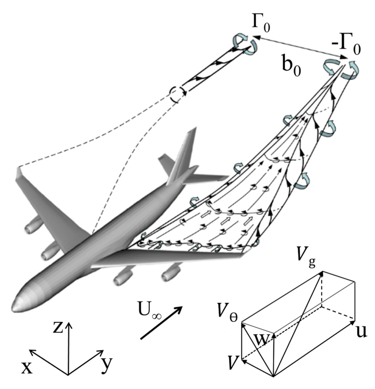
Aircraft wake turbulence, an inevitable byproduct of lift generation during flight, includes tip vortices, boundary layer turbulence, and engine jet wash. As the aircraft flies, the pressure increases below the wing while it decreases above, causing the airflow beneath the wing to curl around the wingtip towards the lower-pressure surface above, thus forming high-speed spiral airflows centered around the wingtips behind the aircraft. The two wingtips correspond to two counter-rotating vortices, with the left wingtip vortex rotating clockwise and the right wingtip vortex rotating counterclockwise, known as tip vortices. The lifecycle of boundary layer turbulence and engine jet wash is short, with a limited action distance, posing little harm to subsequent aircraft. In contrast, tip vortices are characterized by a long duration, wide distribution, and high intensity, significantly impacting the flight safety of following aircraft. This is the focus of the study. Figure 2 illustrates the generation of aircraft wake vortices [23].

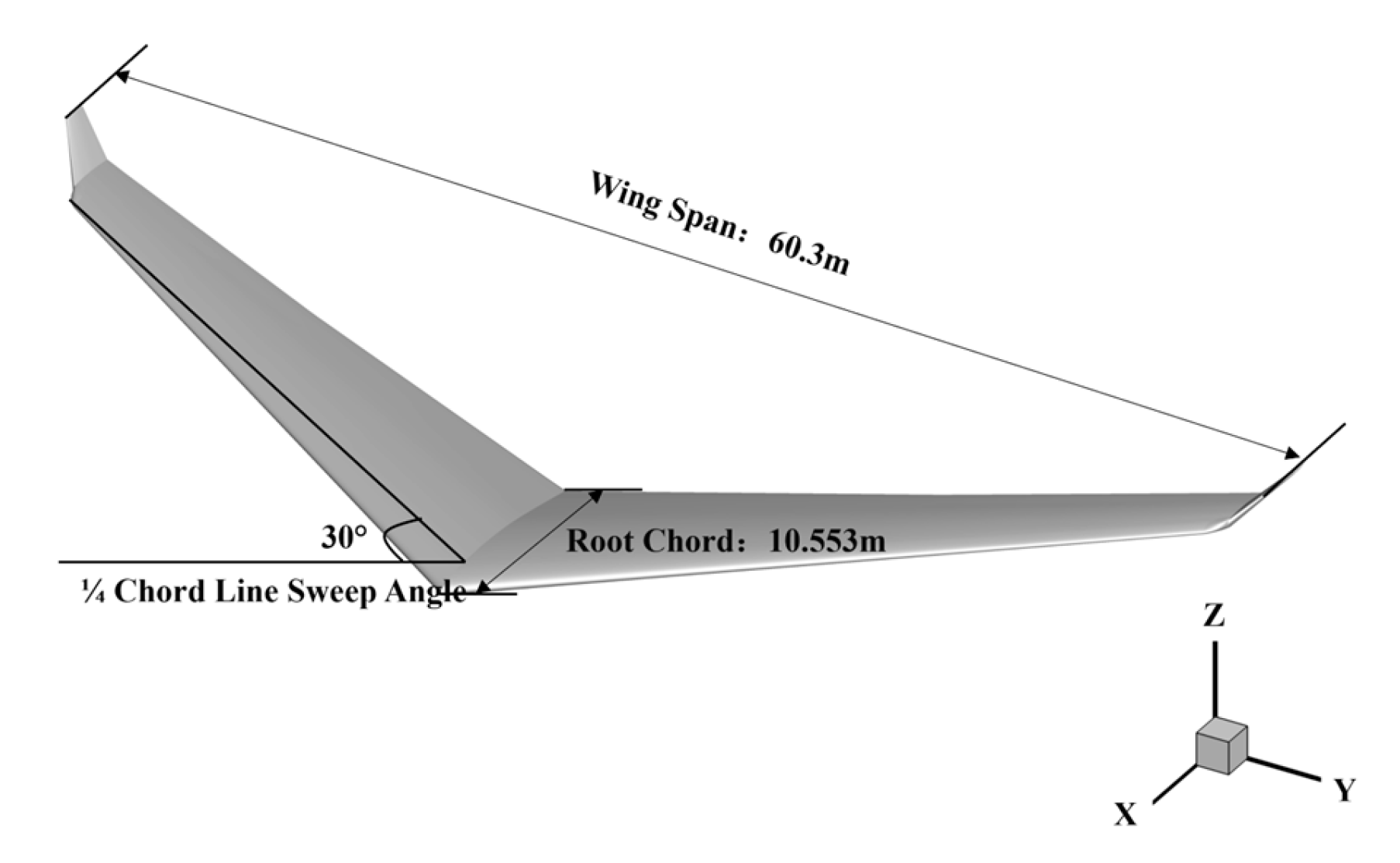
Due to the high frequency of A330 aircraft flights at Chinese airports, the A330-200 was selected as the subject of this study. Wake turbulence is mainly generated by the wingtip effect, where the pressure difference between the upper and lower surfaces of the wing leads to lift, causing lateral airflow at the wingtip and resulting in the formation of high-speed rotating vortices that detach rearward. The fuselage, being a relatively uniform cylindrical structure, may disturb the surrounding airflow; however, its contribution to wake structure is minimal. Even with wingtip integration, additional wingtip effects are limited, as evidenced by studies such as that by Zhang et al. [24], who simplified the fuselage and discussed the evolution of wake vortices formed by the main wing, flaps, and horizontal tail wing. He [19] simplified the fuselage of a B737-800 aircraft and simulated the evolution of wake vortices under different crosswind speeds. Additionally, due to the minor impact of the horizontal tail vortex on aircraft safety after its rapid fusion with the wingtip vortex [25], only the wing section was retained in the computational cases to save computational resources. Furthermore, to simulate the evolution of the wingtip vortex, a portion of the wingtip was retained, as shown in Figure 3.

The final approach is the flight segment, in which an aircraft descends along the landing trajectory and aligns with the runway for landing. Generally, it begins at the final approach fix, where the aircraft maintains its final approach trajectory aligned with the runway centerline extension and starts the approach with a 5.2% descent gradient, equivalent to a 3° glide slope. Due to the relatively stable flight speed, trajectory, and significant overlap within this segment, many scholars have chosen to focus their research on aircraft wake during the final approach phase. However, current research often considers only the ground effect at a single altitude, lacking observational experiments on the impact of ground effects at various altitudes. This makes it challenging to determine at which altitude the ground effect on aircraft wake poses the greatest threat to following aircraft.

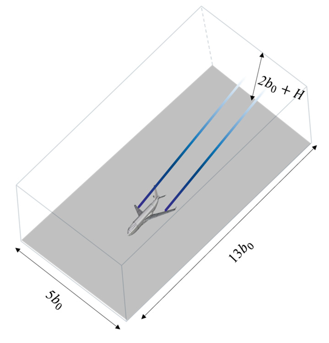
In light of this, and from the perspective of studying the wake dissipation mechanism influenced by continuous variations in approach altitudes, this paper utilizes the User-Defined Function (UDF) secondary development interface tool integrated with the FLUENT 2024 R1 software. It selects the Hallock–Burnham tangential velocity model for the initial model of the wake vortex and structures the flow domain into grids. The maximum grid resolution is set to 0.021 $b_0$, and the minimum grid size in the wake region is 0.1 m × 0.1 m. The calculation domain, where the x-direction is the aircraft’s approach direction, the y-direction is the wingspan direction, and the z-direction is the altitude direction, forms a hexahedral configuration of $5b_0\times 13b_0\times (2b_0+H)$. This is illustrated in Figure 4.

2.1.2. Wake Vortex Tangential Velocity Model

Tangential velocity is a crucial parameter for describing the characteristics of aircraft wake vortices. By the mid-20th century, numerous scholars proposed models for the tangential velocity profiles of aircraft wake vortices either by solving fluid equations or fitting observational data. Among them, the Lamb–Oseen vortex tangential velocity model, the Hallock–Burnham vortex tangential velocity model, and the Adapted Vortex tangential velocity model are the most widely used. The tangential velocities obtained from these models are generally consistent at distances far from the vortex core. Extensive experiments have confirmed that the Hallock–Burnham velocity model largely agrees with the measured data [26], and the Hallock–Burnham velocity model has a simple and unified velocity expression, making it convenient for theoretical analysis and analytical representation. Therefore, the Hallock–Burnham vortex model is used for simulating the induced velocity of aircraft wake, as in Equation (1):

$$V_T\left(r\right)=\frac{{\Gamma }_0}{2\pi r}\frac{r^2}{r^2+r_c}$$

(1)

where $V_T(r)$ is the tangential induced velocity at the point; $r$ is the straight-line distance between the point and the core of the vortex; $r_0$ stands for the vortex core radius; ${\Gamma }_0$ denotes the initial circulation; and $r_{\mathrm{c}}$ is the vortex core radius of the wake vortex.

2.1.3. Aircraft Wake Vortex CFD Numerical Simulation Method

In practical research, if only the time-averaged quantities of turbulent motion characteristics are considered (such as the average velocity field, average forces, etc.), an ensemble average can be performed on the Navier–Stokes (N-S) equations. By solving the time-averaged N-S equations for turbulence, one can quickly simulate the motion of turbulence. This method of averaging the unsteady N-S equations over time to solve for the time-averaged quantities needed in engineering is known as Reynolds-Averaged Navier–Stokes (RANS) [26].

For three-dimensional incompressible fluids, the tensor form of their control equations can be expressed as follows:

$$\frac{\partial \rho }{\partial t}+\frac{\partial \left(\rho \overline{u_i}\right)}{\partial x_i}=0$$

(2)

$$\frac{\partial \left(\rho \overline{u_i}\right)}{\partial t}+\frac{\partial \left(\rho \overline{u_i}\overline{u_j}\right)}{\partial x_j}=-\frac{\partial p}{\partial x_i}+\frac{\partial {\sigma }_{ij}}{\partial x_j}+\frac{\partial }{\partial x_j}\left(-\rho \overline{u{\prime }_{i}u{\prime }_j}\right)$$

(3)

where $p$ is the fluid pressure; $\rho$ is the density of atmospheric turbulence; $x_i$ and $x_j$ are Cartesian coordinates; $u_i$ is the mean velocity component in the $x_i$ direction; $u_j$ is the mean velocity component in the $x_j$ direction; $u_i^{\mathrm{\prime }}$ and $u_j^{\mathrm{\prime }}$ are the fluctuating velocity components that contribute to the stress term in the Reynolds-averaged Navier–Stokes equation; ${\sigma }_{ij}$ represents the components of the stress tensor; and $-\rho \overline{u{\prime }_{i}u{\prime }_j}$ denotes the Reynolds stress term.

After ensemble averaging, the resulting Reynolds-averaged equation includes not only the average pressure forces, average molecular viscous forces, and average mass forces but also an additional stress action $-\rho \overline{u{\prime }_{i}u{\prime }_j}$, namely, the Reynolds stress.

This term is a second-order symmetric tensor, and its expression is as follows:

$$R_{ij}=-\rho \left(\begin{array}{ccc}\overline{u\prime u\prime }& \overline{u\prime v\prime }& \overline{u\prime w\prime }\\ \overline{v\prime u\prime }& \overline{v\prime v\prime }& \overline{v\prime w\prime }\\ \overline{w\prime u\prime }& \overline{w\prime u\prime }& \overline{w\prime w\prime }\end{array}\right)$$

(4)

The existence of the Reynolds stress term makes the equations unclosed, necessitating the introduction of turbulence models to simulate the Reynolds stress in the equations, which then allows for the solution of the average flow field.

Current turbulence models mainly include the Reynolds Stress Model (RSM) or eddy-viscosity closure turbulence models, which encompass zero-equation models, one-equation models, and two-equation models, among others [27].

The $k-\omega$ model has a strong dependence on the distance from the wall, and the SST (Shear Stress Transport) $k-\omega$ model combines $k-\omega$ and $k-\epsilon$, using the $k-\omega$ model near the wall and the $k-\epsilon$ model at the edge of the boundary layer and the free shear layer. Therefore, SST $k-\omega$ has higher calculation accuracy than the standard $k-\omega$ [28,29].

The transport equations of the SST $k-\omega$ model are expressed as follows:

$$\frac{\partial }{\partial t}(\rho k)+\frac{\partial }{\partial x_i}(\rho k{u}_i)=\frac{\partial }{\partial x_i}\left[{\Gamma }_k\frac{\partial k}{\partial x_j}\right]+G_k-Y_k+S_k$$

(5)

$$\frac{\partial }{\partial t}(\rho \omega )+\frac{\partial }{\partial x_i}(\rho \omega u_i)=\frac{\partial }{\partial x_j}\left[{\Gamma }_{\omega }\frac{\partial \omega }{\partial x_j}\right]+G_{\omega }-Y_{\omega }+D_{\epsilon }+S_{\epsilon }$$

(6)

where $G_k$ represents the turbulent kinetic energy generated by the velocity gradient of the laminar flow; $G_{\omega }$ is derived from the $\omega$ (specific rate of dissipation) equation; ${\Gamma }_k$ and ${\Gamma }_{\omega }$ are the diffusion rates for k (turbulent kinetic energy) and $\omega$, respectively; $Y_k$ and $Y_{\omega }$ pertain to the turbulence generated by the diffusion of k and $\omega$; $D_{\omega }$ represents the term for orthogonal divergence; $S_k$ and $S_{\omega }$ are the source terms for turbulent kinetic energy and turbulence dissipation, respectively, acting as customizable terms.

The evolution process of the wake vortex is analyzed using the RANS method, with equation closure conducted by using the SST $k-\omega$ model. The computational domain is a regular hexahedral configuration with dimensions of $5b_0\times 13b_0\times (2b_0+H)$, where the maximum grid resolution is set to 0.021 $b_0$, and the minimum grid size in the wake region is 0.1 m × 0.1 m, resulting in approximately 50 million grid cells. The inlet is set as a velocity inlet, and the outlet as a pressure outlet. The top, left, and right sides are set as symmetric boundaries, and the bottom and the aircraft wing surface are set as non-slip solid walls. The wing is located 3 $b_0$ away from the inlet, 2 $b_0$ away from the top, and 10 $b_0$ away from the outlet. The PISO method is chosen for pressure–velocity coupling, and a tangential velocity model is compiled in the Fluent UDF module for initialization of the wake vortex flow field.

2.2. Extraction of Aircraft Wake Evolution Characteristic Parameters

To understand the evolution patterns of aircraft wake vortices more intuitively and clearly, parameters such as circulation, vorticity, and the Q-criterion are commonly used to quantify wake vortex characteristics.

Circulation is the path integral of fluid velocity (i.e., the tangential velocity of the wake vortex) along a closed curve, typically denoted by $\Gamma$. Its expression is as follows:

$$\Gamma ={\displaystyle \oint { }_L\overrightarrow{\mathrm{U}}·\overrightarrow{ds}}={\displaystyle \oint { }_L\mathrm{U}\cos \theta ds}$$

(7)

where $L$ represents the closed curve, α signifies the angle between the velocity vector and the tangent direction of the point on the line, $\overrightarrow{\mathrm{U}}$ is the velocity vector, $\overrightarrow{ds}$ is the infinitesimal segment vector along the closed path $L$, and $\mathrm{U}\cos \theta$ is the tangential component of the velocity vector $\overrightarrow{\mathrm{U}}$ along the path $L$.

According to the Kutta–Joukowsky theorem [20], the circulation of an aircraft’s wake is related to various factors such as the flight speed and the wing airfoil geometry and distribution. Upstream velocity refers to the airspeed flowing over the aircraft wing surface before the generation of the wake vortex. Since this study only considers still air conditions, the upstream velocity is approximately equal to the aircraft’s final approach speed. When an aircraft with a lift coefficient $C_L$, aspect ratio $A_R$, and wingspan $B$ flies at a speed $V$, the lift it generates equals the momentum flux of the rolled-up wake vortices. This can be expressed as

$$\frac{\rho C_L}{2A_R}{B}^2{V}^2=\rho V{b}_0{\Gamma }_0$$

(8)

$$b_0=Bs$$

(9)

where $b_0$ is the initial spacing between the rolled-up vortices; s is the load factor along the wingspan direction (under the assumption of elliptical wings [5], which is approximately true for commercial airliners, and is about $\pi /4$); $\rho$ is the air density.

Thus, the initial circulation ${\Gamma }_0$ of the aircraft’s wake can be described as follows:

$${\Gamma }_0=\frac{C_{L}VB}{2s{A}_R}$$

(10)

$${\Gamma }_0=\frac{{\mathrm{n}}_{\mathrm{y}}Mg}{\rho sBV}=\frac{4Mg}{\rho \pi BV}$$

(11)

where M is the mass of the aircraft, $\rho$ is the air density, $V$ is the flight speed, and $s$ is the wing shape parameter, which is related to the wing shape. For a rectangular wing, $s$ can be taken as $\frac{\pi }{4}$, and ${\mathrm{n}}_{\mathrm{y}}$ is the load factor. Since the calculation process does not consider rapid maneuvers such as sharp turns and rapid climbs, it is simplified and set to 1.

In numerical simulations, the calculation method for circulation involves taking the average of the area integrals of vorticity on 11 circular planes (centered at the vortex core, with radii ranging from 5 to 15 m) [30], then normalizing it with the initial circulation for dimensionless representation, as in Equation (12):

$${\Gamma }_{5-15}^{\ast }=\frac{1}{11}{\displaystyle \sum _{r=5}^{15}({\displaystyle \underset{0}{\overset{r}{\int }}\omega dA})}/{\Gamma }_0$$

(12)

Vorticity is another crucial parameter characterizing the strength of aircraft wake vortices, with its physical significance being the description of the curl of the velocity vector of the fluid. In the case of a two-dimensional planar flow field, since vorticity has components in only one direction, it can be represented by the component of vorticity in the Z direction, as in Equation (14):

$$\omega ={\omega }_z=\partial v/\partial x-\partial u/\partial y$$

(13)

The Q-criterion is a physical criterion used to describe the structure and evolution of vortices in fluid flow by calculating the fluid velocity gradient tensor, aiming to quantify the presence and strength of vortices in the flow field using the eigenvalues of this gradient tensor. Unlike traditional velocity vector fields, the Q-criterion can intuitively display details such as vortices and boundary layers, and it uses the eigenvalues of the gradient tensor to assess the intensity of eddies. The two-dimensional dimensionless Q-criterion for the $oxz$ plane can be expressed as follows:

$$Q=-\frac{1}{2}[{(\frac{\partial u}{\partial x})}^2+{(\frac{\partial v}{\partial z})}^2]-\frac{\partial u}{\partial z}\frac{\partial v}{\partial x}$$

(14)

where $u$ and $v$ represent the velocity components in the $x$ and $z$ directions, respectively. When the Q value is greater than 0, the point can be considered as part of a vortex. This approach effectively highlights regions in the flow where the rotation dominates the strain, thus identifying the core areas of vortices.

2.3. Correlation Analysis

To investigate the effect of the initial altitude at which aircraft wake vortices are generated on their evolution, an analysis of the correlation between altitude and extracted wake vortex parameters was conducted using the Pearson correlation coefficient. According to Figure 5, there is a positive correlation coefficient of 0.22 between altitude and the initial circulation of the aircraft wake vortex, indicating that as altitude increases, the initial circulation of the wake vortex also tends to increase. Moreover, the correlation coefficient between altitude and the Q-criterion value of the aircraft wake vortex is −0.77, demonstrating a strong negative correlation. This suggests that as altitude increases, the Q-criterion value of the aircraft wake vortex tends to decrease, indicating that the evolution of aircraft wake is significantly influenced by altitude.

2.4. Wake Parameter Prediction Model Based on PA-TLA

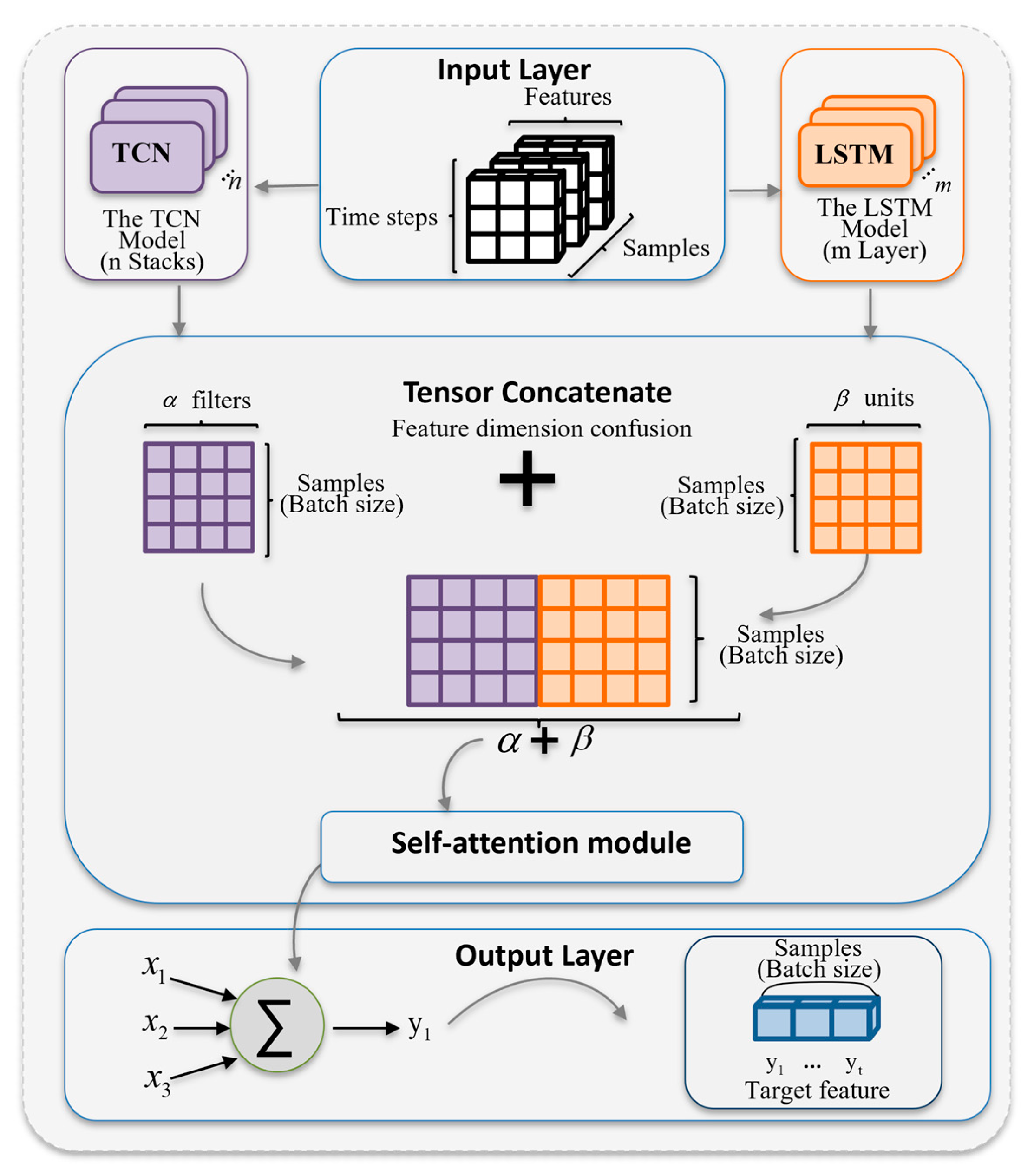
TCNs (Temporal Convolutional Networks) and LSTM (Long Short-Term Memory) each have their advantages and are suitable for different scenarios. TCNs employ a multi-stacked, dilated causal convolution process to focus on the local features of time series data. On the other hand, LSTM uses gated units to maintain a global perception of the entire sequence, storing previous information in hidden layers to transmit contextual information. However, classical serial hybrid framework models increase the demand for computational memory and time, neglecting the increase in the number of model parameters and complexity, leading to higher computational costs during training and reduced timeliness. Therefore, this study proposes a hybrid deep learning model based on a parallel architecture that combines the neural networks of Temporal Convolutional Networks (TCNs) and Long Short-Term Memory (LSTM) through a tensor fusion module based on attention mechanisms for predicting aircraft wake vortex parameters and safety intervals. The TCN and LSTM operate independently to capture key features, such as long-term dependencies and contextual information. Finally, through tensor fusion based on the attention mechanism, the output matrices of the TCN and LSTM are assigned different attention weights. These are dynamically weighted according to task requirements and merged in the feature dimension to achieve feature information fusion. The depth of the model in this parallel mode is only affected by the depth of each individual network layer. The structure of the model is illustrated in the figure, and this configuration is referred to as the Parallel Architecture LSTM-TCN-Attention (PA-TLA), as shown in Figure 6.

2.4.1. Sequence Space Feature Representation Based on TCN

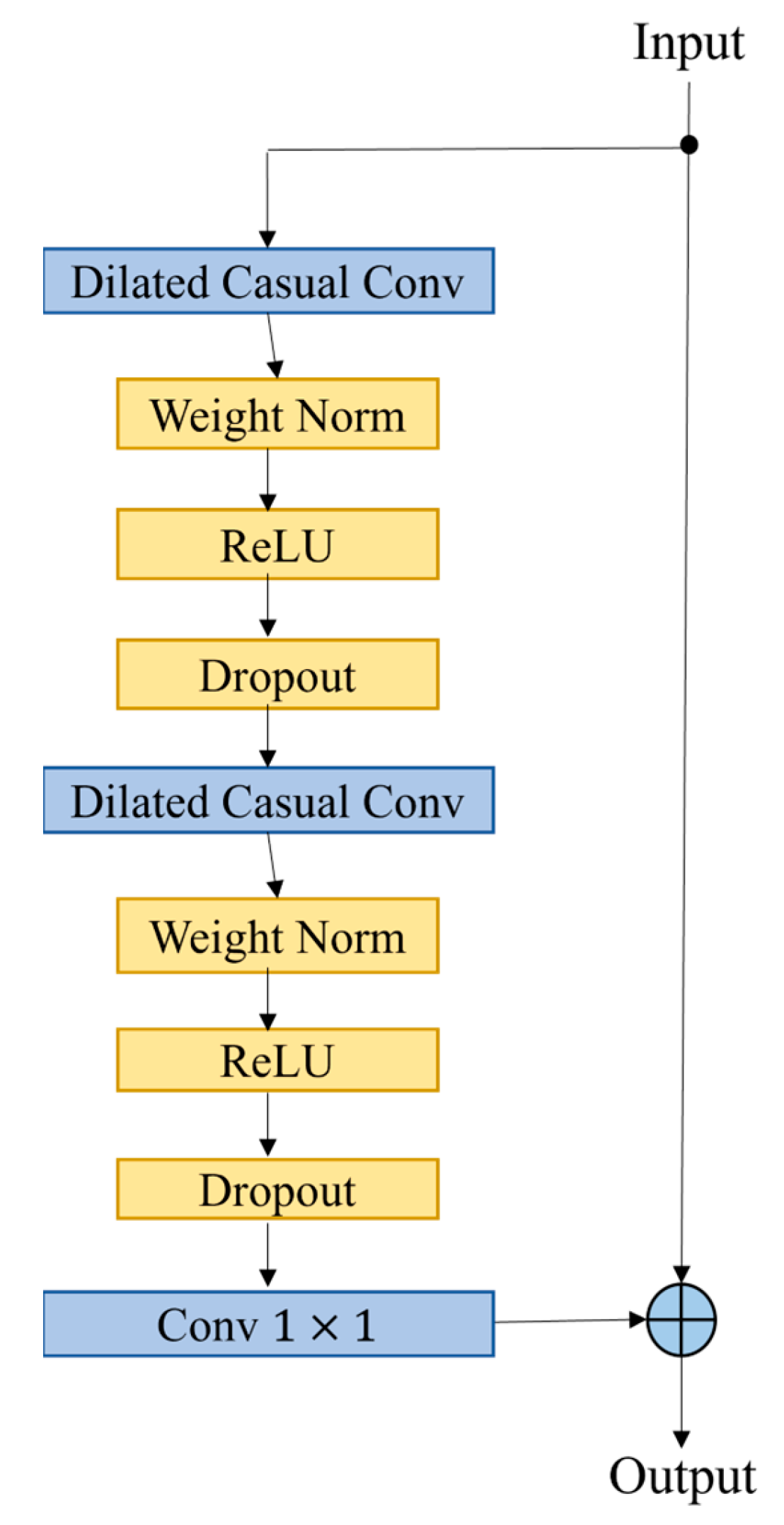
The Temporal Convolutional Network (TCN) is a model based on the CNN architecture designed for processing time series data. In this study, we employ the TCN network as a branch of the PA-TLA prediction network to extract global spatial features of sequences. The TCN consists of a stack of multiple residual units. Each residual module includes two convolutional units and a nonlinear mapping unit, comprising one-dimensional dilated causal convolution, weight normalization, a ReLU activation function, and a dropout operation.

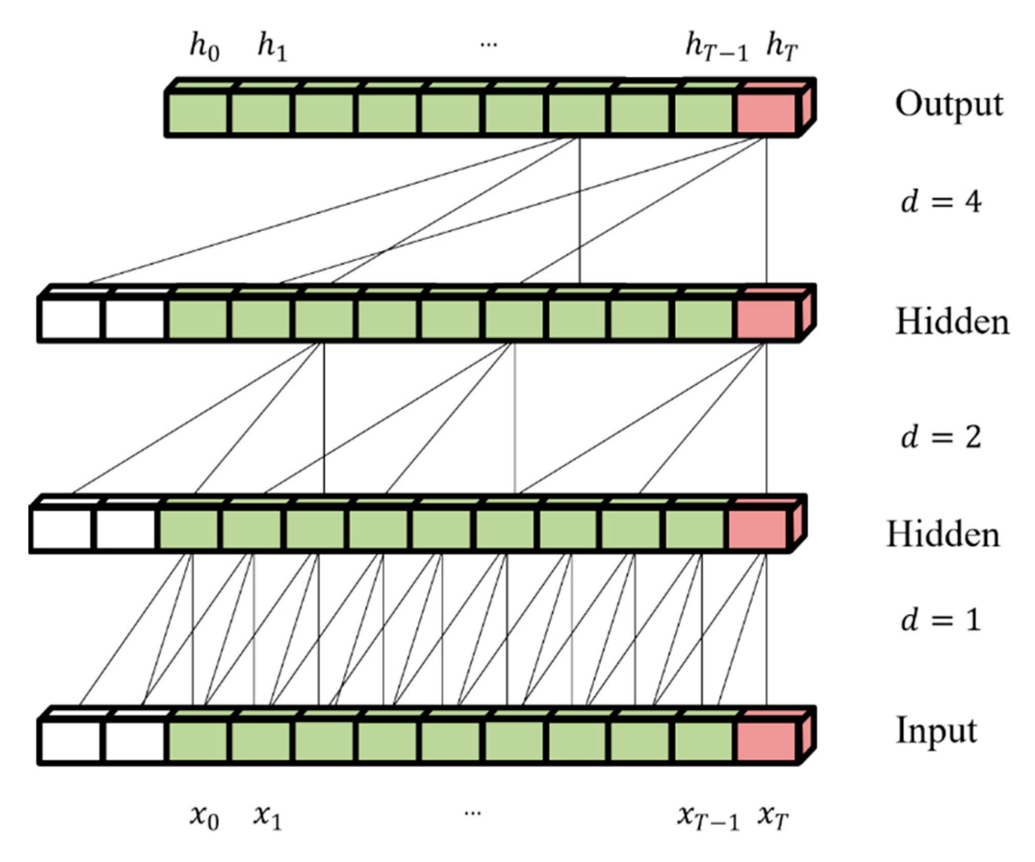
The TCN mainly includes three basic features: causal convolution, dilated convolution, and residual connections. The dilated causal convolution illustrated in Figure 6 is obtained by convolving the input with a causal relationship to generate network output. In sequence modeling, causal convolution means that the current moment $\mathrm{T}$ is only related to the inputs at moment $\mathrm{T}$ and before. Its mathematical form is described below.

The TCN primarily features three fundamental characteristics: causal convolution, dilated convolution, and residual connections. In sequence modeling, causal convolution ensures that the output at the current time T is only related to inputs at time T and prior times. The mathematical form is described as follows:

$$h_r=f(|x_1|,|x_2|,|\cdots |,|x_T|)$$

(15)

where $x_T$ is a one-dimensional vector containing $n$ features, and $h_r$ is the variable to be predicted. $f$ is the function that establishes the relationship between $x_T$ and $h_r$. Causal convolution is a unidirectional structure, ensuring the sequentiality of data processing by handling the values at moment $t$ and only using data from before moment $t$. For a one-dimensional series input, the dilated convolution operation, $F(S)$ on its elements and the filter $f:\{0,\dots ,\mathrm{k}-1\}$ are defined as follows:

$$F(S)=(x\ast df)(s)=\sum _{i=0}^{k-1}f\left(i\right)·x_{s-d·i}$$

(16)

Given $s$ as the input sequence information, $d$ as the dilation factor, and $k$ as the size of the filter, $s-d·i$ represents the location of certain information in the history. As the dilation factor $d=(\mathrm{1,2},4)$ increases, the receptive field of the TCN increases, leading to an increase in the amount of information received. The expanded convolution structure is shown in Figure 7.

Residual connections have proven their effectiveness in training deep networks by allowing information to be transmitted across layers. Each residual block includes a branch that leads out a series of transformations $F$ whose outputs are added to the input X of the block:

$$\beta =Activation(X+F(X))$$

(17)

As shown in Figure 8, within the residual block, the TCN comprises two layers of dilated causal convolutions and nonlinear processing, where Rectified Linear Units (ReLU) are used. For normalization, weight normalization is applied to the convolutional filters. Additionally, after normalization through dilated convolution, a spatial dropout is incorporated in each layer to deactivate some neurons, thus avoiding overfitting.

2.4.2. LSTM

Long Short-Term Memory (LSTM) neural networks are an optimized variant of Recurrent Neural Networks (RNNs), designed to address the issues of vanishing and exploding gradients that are present in traditional neural networks. LSTM networks aim to mitigate long-term dependency problems, making them particularly suitable for tasks that require learning from sequences of data over long periods. They have been refined and expanded by numerous scholars in various works and have shown impressive performance across a wide range of time series problems.

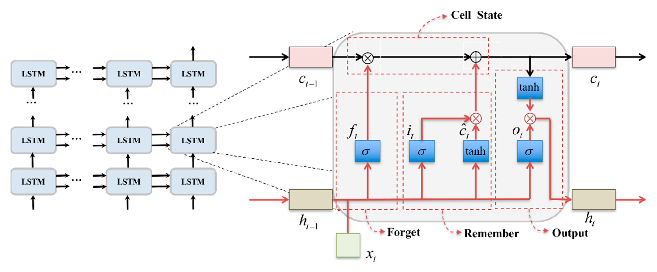
A LSTM neural network unit includes three gates: the input gate, output gate, and forget gate. These gates work together to regulate the flow of information into and out of the cell, deciding what to keep in or omit from the cell’s state. The architecture of a basic unit and the LSTM network architecture are depicted in the figures (not provided here). As represented in Figure 9 (hypothetically, since the figure is not displayed), the equations for a LSTM unit are as follows:

$$f_t=\sigma (W_f\cdot [h_{t-1},x_t]+b_f)$$

(18)

$$i_t=\sigma (W_i\cdot [h_{t-1},x_t]+b_i)$$

(19)

$${\tilde{C}}_t=\tanh (W_C\cdot [h_{t-1},x_t]+b_C)$$

(20)

$$o_t=\sigma (W_o\cdot [h_{t-1},x_t]+b_o)$$

(21)

$$C_t=f_t\odot C_{t-1}+i_t\odot {\tilde{C}}_t$$

(22)

$$h_t=o_t\odot \tanh (C_t)$$

(23)

where $W_f, W_i, W_C$, and $W_o$ represent the weight matrices associated with the forget gate, input gate, candidate values (for updating the cell state), and output gate, respectively. These matrices play crucial roles in determining the flow and transformation of information within the LSTM cell. $h_{t-1}$ is the hidden state from the previous time step, carrying information from earlier in the sequence. $x_t$ is the input information at the current time step, introducing new information to be processed. $b_f,b_i,b_C$, and $b_o$ are biases that adjust the output of their respective gates and candidate cell state update mechanisms, adding another level of adaptability to the model. The cell states, $C_t$ and $C_{t-1}$, represent the memory of the LSTM cell. $C_t$ is the current cell state, $C_{t-1}$ is the cell state from the previous time step, $\sigma$ represents the sigmoid activation function, which is used to compute the output of gates, and tanh represents the hyperbolic tangent function, which is used to compute the output of the candidate memory state. $f_t$ denotes the output of the forget gate, $i_t$ denotes the output of the input gate, and $o_t$ denotes the output of the output gate.

These states are critical for the LSTM’s ability to carry information across long sequences, allowing the network to remember and forget information selectively. ${\tilde{C}}_t$ represents the candidate cell state, which is a combination of the current input $x_t$ and the previous hidden state $h_t$. It suggests potential updates to the cell state, providing the model with the option to incorporate new information based on the input and the LSTM’s memory. The final decision on which memories to keep or discard—and how much of the new candidate state to add to the existing cell state—is made through the input and forget gates, guided by the LSTM’s learned parameters. This architecture enables LSTM networks to decide what information is valuable and should be retained over long sequences, making them exceptionally suited for tasks that require understanding and processing sequential data with complex, long-range dependencies.

2.4.3. Attention-Based Tensor Concatenation Module

From Figure 1, it can be seen that the PA-TLA (Parallel Architecture LSTM-TCN-Attention) proposed in this paper is composed of two independent models and a specialized architecture. One is a TCN (Temporal Convolutional Network) with n layers, and the other is a LSTM (Long Short-Term Memory) network with m layers. These two multilayer networks operate independently but share the same input data. Afterward, a tensor fusion module combines the output results of the two networks. The principle is as follows:

$$y_i=RELU(w\sum _{i=1}^{o+\xi }{x}_i+b)$$

(24)

where $y_i$ represents the target output value, $x_i$ is the input, $w$ denotes the weight values, $b$ stands for the bias values, $RELU$ refers to the Rectified Linear Unit, $o$ is the number of filters in the last stack of the TCN, and $\xi$ is the number of units in the last layer of the LSTM. Due to the lack of sensitivity to the temporal features within the sequence data of LSTM and TCN, they fail to capture the intrinsic connections within the data, limiting their ability to extract and learn important feature information, which is not conducive to further improving the model’s prediction accuracy. Therefore, this paper introduces a self-attention mechanism, connecting different positions within the sequence to enhance the model’s ability to capture key temporal feature information. First, for each output, the corresponding Query, Key, and Value vectors need to be calculated through three different fully connected layers, as shown in the following equation:

$$\begin{array}{c}{Q}_i=W_Q{y}_i+b_Q\\ K_i=W_K{y}_i+b_K\\ V_i=W_V{y}_i+b_V\end{array}$$

(25)

where $W_Q,W_K,W_V$ represent the weight matrix, and $b_Q,b_K,b_V$ are the bias term. Attention scores $e_{ij}$ are computed using the query and key as follows, where $b_{att}$ is the bias term, $W_{att}$ is the weight matrix, and $\tanh$ represents a nonlinear activation function. Then, the softmax function is applied to normalize the attention scores across all time steps, resulting in the final attention weights $a_{ij}$, as shown in the following equation:

$$a_{ij}=\frac{exp(e_{ij})}{{\displaystyle \sum _{k=1}^N}exp(e_{ik})}$$

(26)

Finally, the final output is obtained by calculating the weighted sum, as in the following equation:

$$z_i={\displaystyle \sum _{j=1}^N{a}_{ij}}{V}_j$$

(27)

3. Experiments

3.1. Material Preparation

3.1.1. Wake Vortex CFD Numerical Simulation Data

In experiments involving numerical simulation of aircraft wake vortex dissipation, data on the evolution of vortices from an A330-200 aircraft within a height range of 5–300 m above ground level (with 1 m intervals) were collected. This included aircraft and environmental parameters, which are detailed in

Table 1. Relevant parameters of the Airbus A330-200 model.

Environmental Parameter
Ambient Temperature	20 °C
Atmospheric Pressure	1 atm
Air Density	1.225 kg/m3
Dynamic Viscosity	1.81 × 10−5 Pa·s
Turbulence Intensity	1.86%
Aircraft Parameters
Wingspan	60.3 m
Maximum Landing Weight	182,000 kg
Speed	72 m/s
Initial Vortex Circulation	427 m2/s
Vortex Core Radius	3 m ≈ 0.052B
Initial Vortex Spacing	47.36 m ≈ Bπ/4
Characteristic Speed	1.436 m/s
Characteristic Duration	33 s

. Through these complex numerical simulations, a total data volume of approximately 14.3 TB was generated, detailing the evolution of the wake vortex.

The vortex core radius ($r_c$) is the radial distance from the center of the vortex core to the point in the nearby flow field where the tangential velocity reaches its maximum value. It is an important parameter for measuring the distribution of aircraft wake vortices. In numerical simulation studies of wake vortices, the selected values [5] for the vortex core radius vary among different references. For ideal aircraft wake vortices, the range of values for the vortex core radius generally lies between $r_c/b_0=1\%-7\%$. This paper references the value for $r_c/b_0$ used by Holzäpfel in their research, which is 5.2%. The air density is assumed to be constant at 1.225 kg/m³, following the standard atmospheric pressure for ideal gases [31,32]. According to the Biot–Savart law, the induced velocity at the core when the wake vortex is fully rolled up (i.e., the characteristic velocity) $w_0$ is given by Equation (28):

$${\omega }_0=\frac{{\Gamma }_0}{2\pi b_0}=\frac{8Mg}{\rho {\pi }^3{B}^{2}V}$$

(28)

The characteristic time $t_0$ for the wake vortex to descend $b_0$ distance from its initial position at a constant velocity of ${\omega }_0$ is

$$t_0=\frac{b_0}{{\omega }_0}=\frac{\rho {\pi }^4{B}^{3}V}{32Mg}$$

(29)

Figure 10 shows the variation in wake vortex vorticity and tangential velocity over time under calm wind conditions. The analysis reveals that in the initial stage after detachment, the wake vortex has a relatively small impact range, forming a sudden change area of vorticity only near the vortex core, with a vorticity extreme point appearing at the center of the vortex core, approximately 12 s⁻¹. Outside the vortex core area, as the radial distance from the vortex center increases, the vorticity gradually decreases. Subsequently, influenced by gravity and the mutual induction between wake vortices, the wake vortex gradually shows a downward trend, and the affected area of the wake vortex begins to expand. By 33 s, under calm wind conditions, the vorticity cloud map of the wake vortex shows that the impact range of the wake vortex has significantly expanded compared to the initial stage, but the maximum vorticity value at the vortex core has significantly decreased. Around 66 s, the interaction effect between wake vortices gradually strengthens, and a merging trend appears in the flow field surrounding the wake vortices.

3.1.2. CFD Data Validation

Using LIDAR data to validate CFD data ensures that the model can accurately predict the behavior of wake vortices. The study employed the Wind3D 6000 aviation meteorological LIDAR developed jointly by the Ocean University of China and Qingdao Ray Measurement and Control Technology Co., Ltd., Qingdao, China. This device can continuously measure three-dimensional vertical wind profiles, wind speed, and wind direction, obtaining high-precision real-time wind field data.

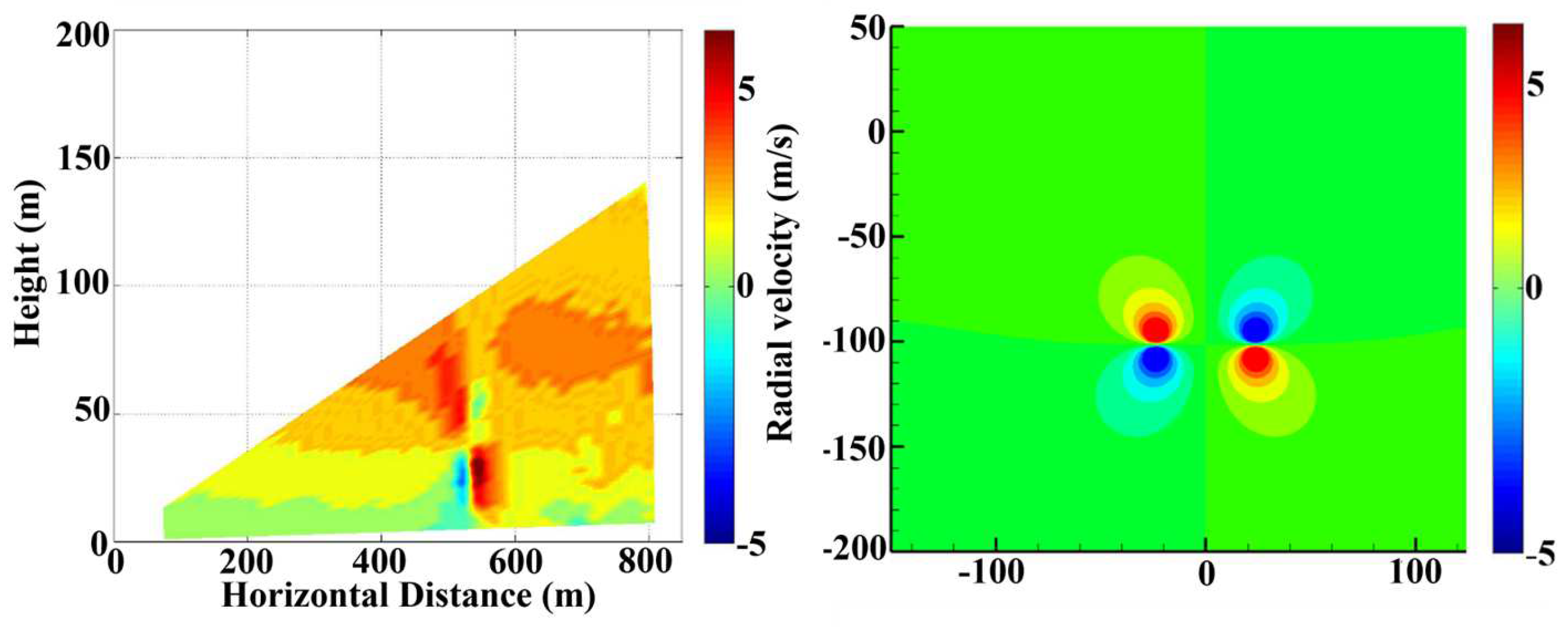
According to the Beaufort Scale, wind speeds below force 1 are defined as calm, which corresponds to wind speeds less than 1.5 m per second. The evolution data of the wake vortex for the A330 model are filtered at wind speeds close to calm (below 1.5 m/s), and the numerically simulated wake vortex radial velocity is compared with the laser radar-detected wake vortex radial velocity. As shown in Figure 11, the left is a mapping of actual LIDAR data, with the LIDAR placed 350 m from the runway; the right is a mapping of data obtained from numerical simulations. It shows two sets of velocity pairs in opposite directions, with the maximum radial velocity around 5 m per second. The distribution of the velocity pairs satisfies rotational symmetry. Both the x-axis and y-axis are in meters; the x-axis represents the distance extending horizontally from the vortex center, and the y-axis represents the distance extending vertically from the vortex center.

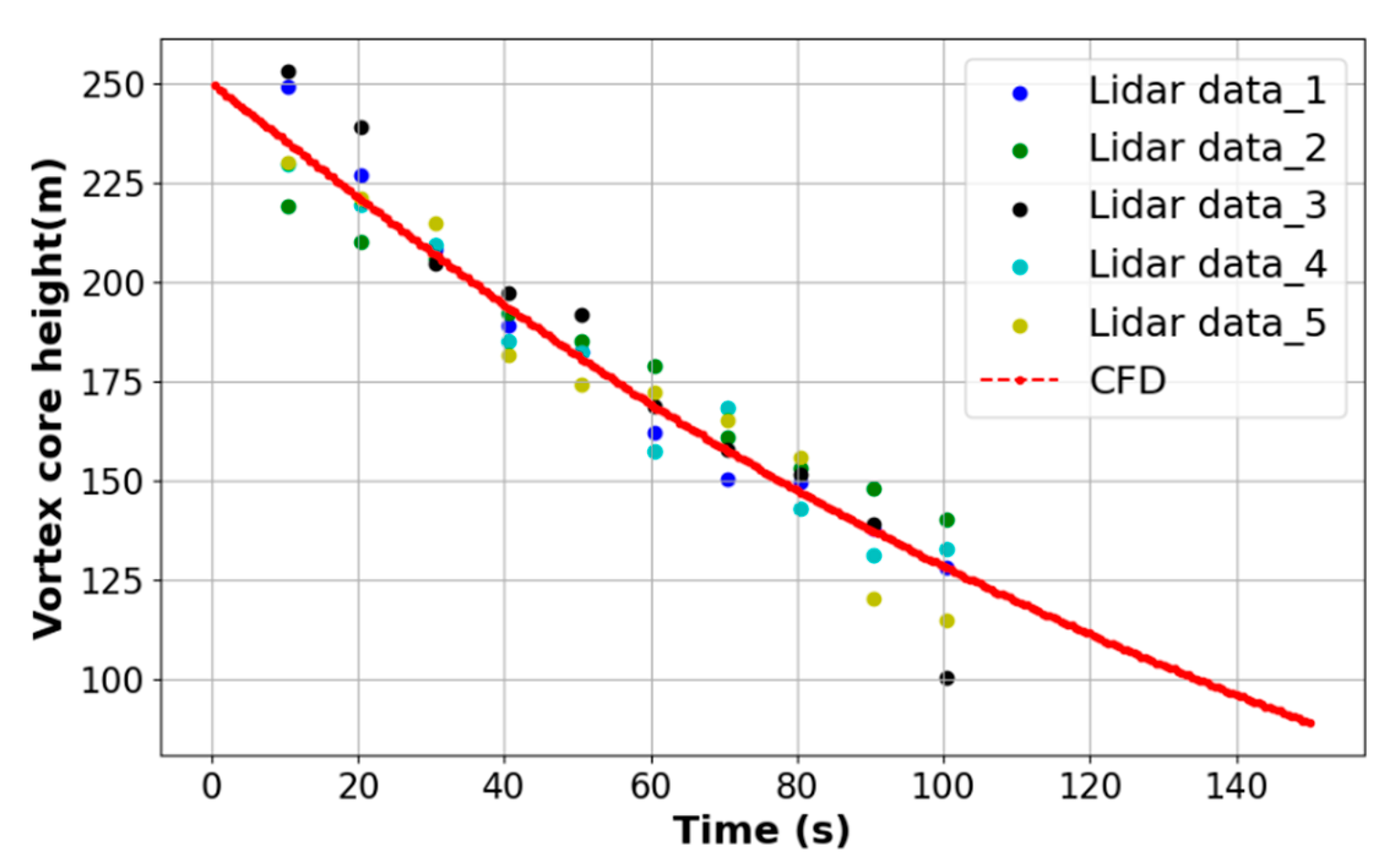
We selected five LIDAR datasets of the A330-200 model under near-calm wind conditions (less than 2 m/s), extracted the evolution patterns of the vortex core height of the aircraft wake, and compared these with the evolution patterns of the vortex core height obtained from the CFD data at corresponding times, as shown in Figure 12. The results indicate that the CFD evolution data obtained through simulations closely match the aircraft wake evolution patterns detected by the LIDAR in the field.

3.2. Evaluation Criteria

In this study, we use normalized mean absolute error (MAE), normalized mean squared error (MSE), normalized root mean squared error (RMSE), and R² as evaluation metrics to assess the predictive performance of the model. Furthermore, the MSE is used as a measure of accuracy during model training. The MAE provides a direct average margin of error, as shown in Equation (30). The MSE highlights large errors, as seen in Equation (32). The RMSE presents the error in the same units as the predicted value, providing interpretability, as shown in Equation (31). R² evaluates the overall explanatory power of the model, as seen in Equation (33).

$$MAE=\frac{1}{n}\sum _{i=1}^n|y_i-{\widehat{y}}_i|$$

(30)

$$RMSE=\sqrt{\frac{1}{n}\sum _{i=1}^n{(y_i-{\widehat{y}}_i)}^2}$$

(31)

$$\mathrm{MSE}=\frac{1}{n}\sum _{i=1}^n{(y_i-{\widehat{y}}_i)}^2.$$

(32)

$$R^2=1-\frac{{\mathsf{\Sigma }}_{i=1}^n{(y_i-{\widehat{y}}_i)}^2}{{\mathsf{\Sigma }}_{i=1}^n{(y_i-{\overline{y}}_i)}^2}$$

(33)

where ${\gamma }_i$ is the predicted value; ${\widehat{y}}_i$ is the actual value; n is the number of samples.

3.3. PA-TLA Parameter Configuration

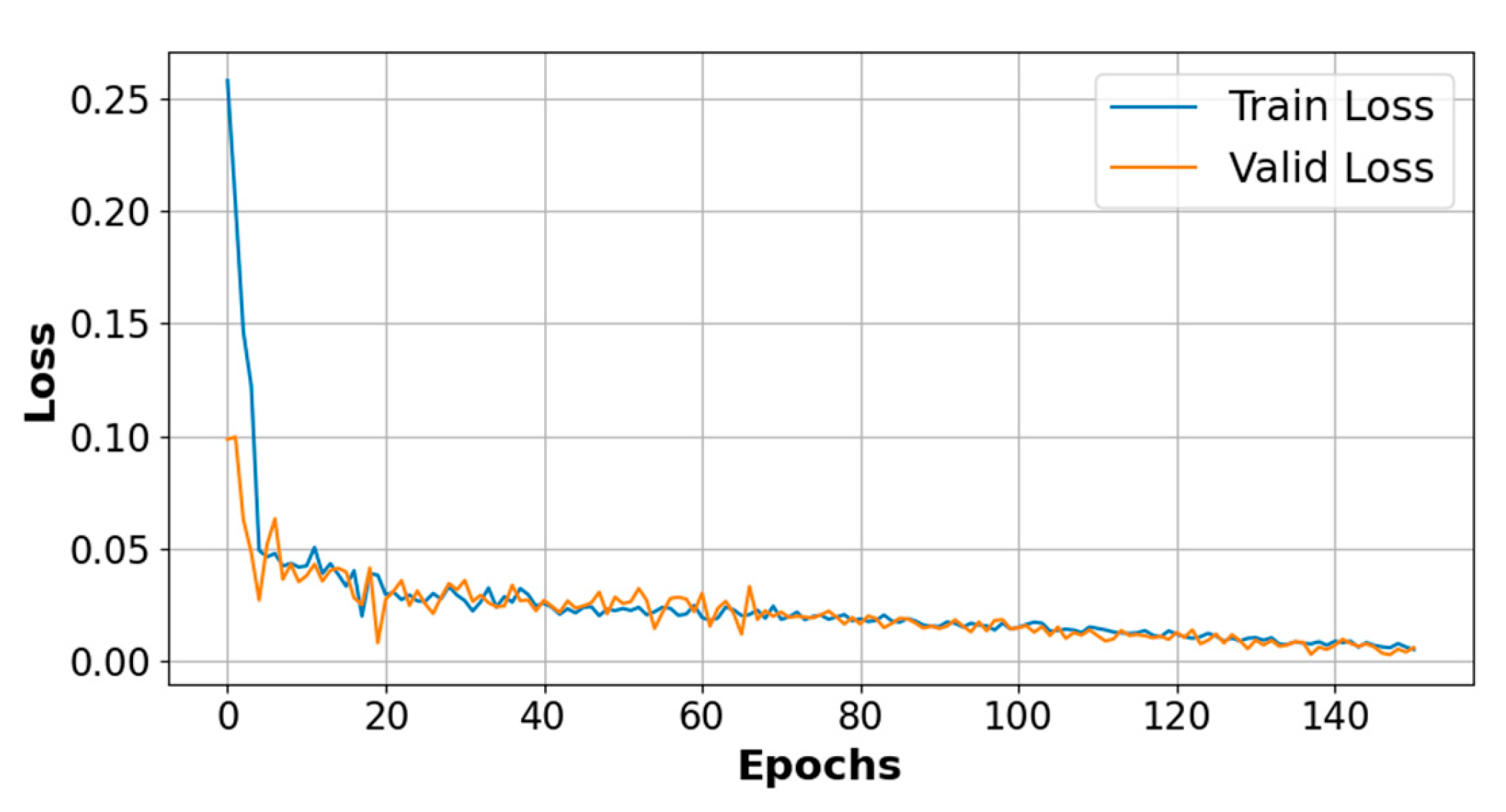
PA-TLA is a parallel architecture composed of two layers of convolutionally stacked TCNs (Temporal Convolutional Networks) and three layers of LSTM (Long Short-Term Memory). We set the time step to 12, use the Adam optimizer during training, employ MSE (mean squared error) as the loss function, maintain a batch size of 64, and run the model for 150 epochs. As depicted in Figure 13, the loss on the training and validation datasets evolves throughout the training epochs. Clearly, after all iterations, the model exhibits no signs of overfitting.

3.4. Results Analysis

3.4.1. Wake Evolution Prediction Model Based on PA-TLA

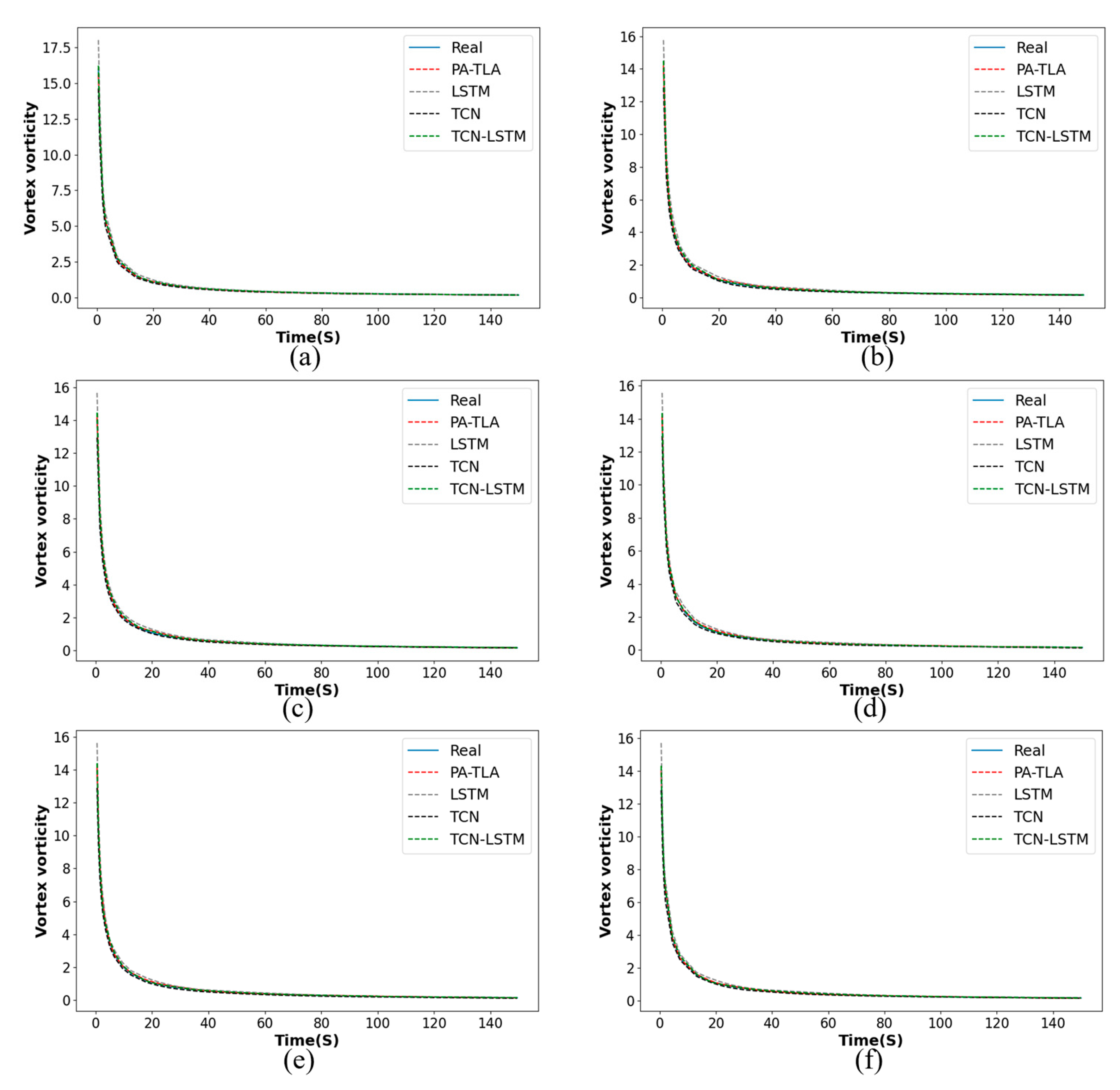
To further demonstrate the effectiveness of the PA-TLA, we constructed a TCN-LSTM structure composed of a two-layer convolutional stacked TCN and a three-layer LSTM in series, as illustrated in Figure 14a–f. This figure shows a comparison of predicted and actual vorticity characteristic parameters for four models, all of which exhibit high levels of fit: PA-TLA, TCN-LSTM, LSTM, and TCN.

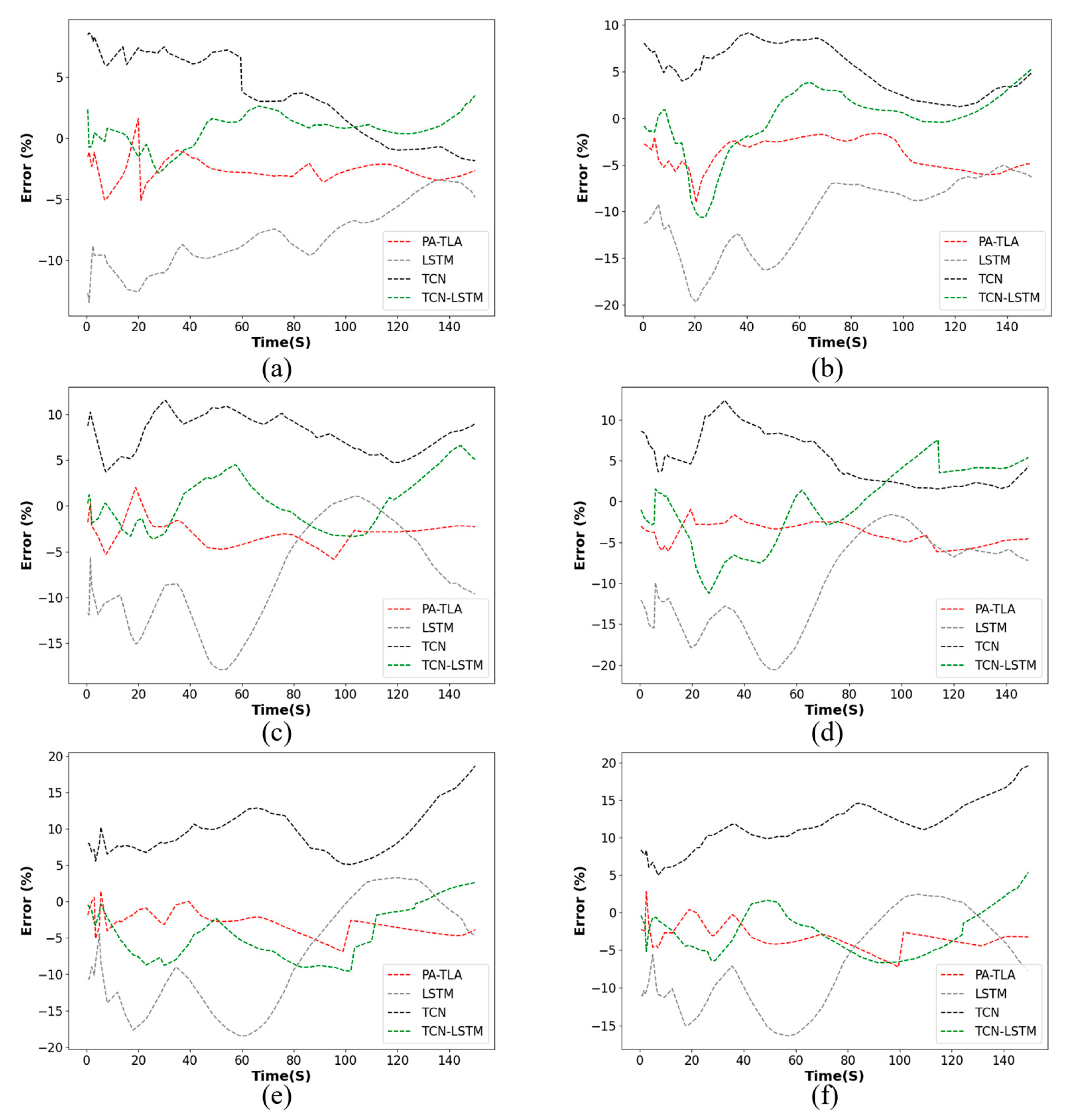
To further observe the prediction errors of the four models, Figure 15 presents the relative error plots for the predicted vorticity characteristic parameters. This figure demonstrates the models’ performances at various distances, with time on the x-axis and vorticity on the y-axis. It is evident that the TCN, with its capability to perceive spatial features of the sequence, performs better in terms of relative error compared to LSTM. Both PA-TLA and TCN-LSTM, which integrate the spatial feature perception of the TCN with the temporal feature perception of LSTM, show good performance in predicting aircraft wake characteristic parameters, with PA-TLA outperforming TCN-LSTM in relative error.

Table 2. The prediction results of the three models on the testing set.

Feature	Model	MSE	MAE	RMSE	R2
Q-criterion	TCN	0.239	0.086	0.149	97.891
	LSTM	0.274	0.091	0.189	97.147
	TCN-LSTM	0.205	0.073	0.134	98.712
	PA-TLA	0.191	0.066	0.129	99.161
Vorticity	TCN	0.109	0.123	0.331	97.163
	LSTM	0.113	0.136	0.335	96.934
	TCN-LSTM	0.085	0.096	0.267	97.934
	PA-TLA	0.079	0.088	0.252	98.256
Circulation	TCN	12.749	2.968	4.192	96.736
	LSTM	13.141	3.352	4.753	96.356
	TCN-LSTM	10.356	2.105	3.206	97.846
	PA-TLA	9.682	1.956	3.075	98.158

reveals that across different heights, the models predict the wake circulation, vorticity, and Q-criterion. PA-TLA and TCN-LSTM outperform LSTM and the TCN on all error metrics, exhibiting a lower mean squared error (MSE), mean absolute error (MAE), and root mean square error (RMSE) and a higher coefficient of determination (R²), indicating superior model fit and significantly enhanced predictive accuracy on this dataset. Moreover, compared to TCN-LSTM, PA-TLA shows an average reduction in MSE of 6.80%, in MAE of 7.70%, and in RMSE of 4.47% and an average increase in R² of 0.36%. The training time for the PA-TLA model is approximately 144 min, and prediction time is about 292 s, whereas the TCN-LSTM requires 201 min for training and 380 s for prediction, demonstrating a 28% improvement in training efficiency and a 35% increase in prediction efficiency for the parallel structure over the serial model structure.

3.4.2. Analysis of Near-Ground Phase Wake Vortex Evolution Characteristics Combining Numerical Simulation and PA-TLA Model

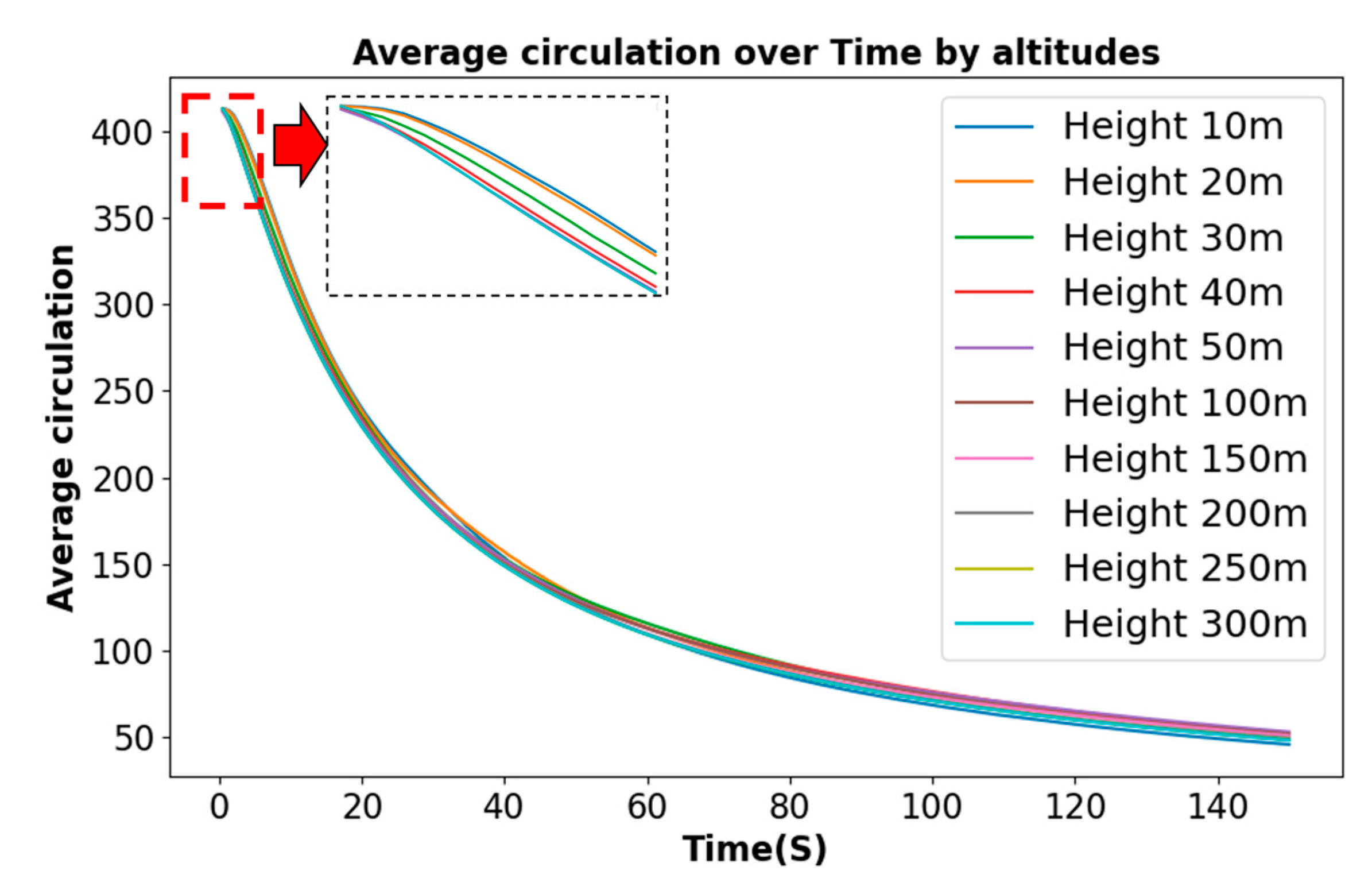
The experiment, focusing on the A330-200 model, predicts different stages of wake evolution in the near-ground phase through the proposed PA-TLA model, selecting circulation and vortex core position as parameters for quantitative analysis of vortex characteristics. Figure 16 shows that at different height conditions, the model-predicted average vortex circulation follows a negative exponential decay rule through the initial stage, rapid decay, and gradual transition to a stable evolution pattern. From 0 s to 10 s, the initial circulation of the aircraft wake decays at an accelerating rate due to turbulent dissipation and viscous effects, as clearly depicted in Figure 17. During the rapid decay phase of 10–20 s, air viscosity causes circulation within the vortex to diffuse and dissipate radially and axially through friction and mixing processes within micro-scale vortices, accelerating the reduction of circulation. Moreover, for low altitude vortices, the shear layer thickness between them and the ground is thinner, making the viscous effects more significant and further intensifying the dissipation of circulation. However, after 80 s, as the vortex structure gradually diffuses, part of the circulation may reorganize into secondary vortices or vortex filaments, forming more complex vortex structures. Despite the potential continued decrease in circulation, the change in vortex morphology can slow its further decay. From 10 m to 50 m, as the height increases, the effect of ground influence weakens, increasing the rate of wake decay. From 50 m to 300 m, the rate of wake decay is almost consistent.

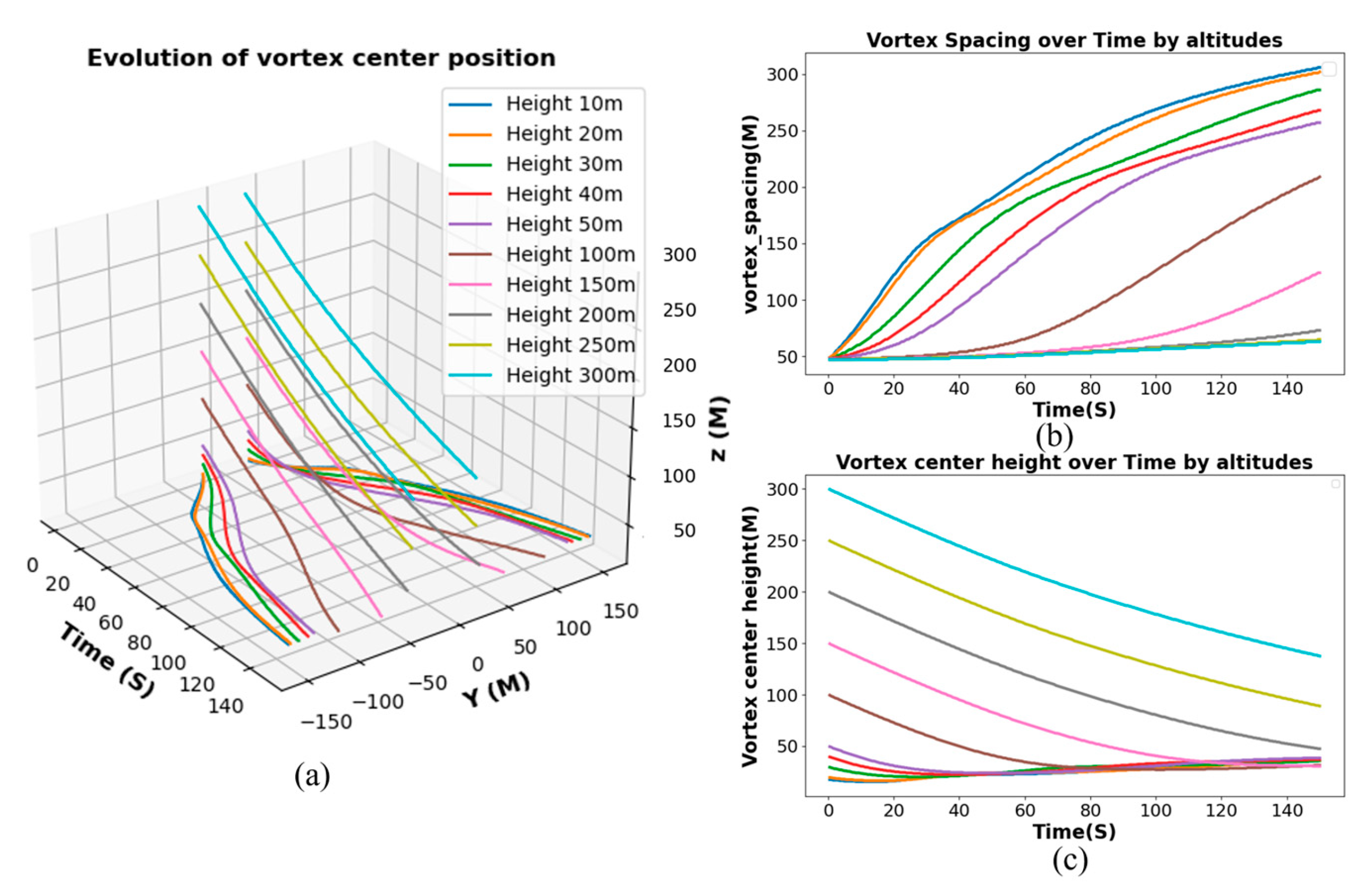
The time-dependent evolution trend of the vortex core position at different initial heights is shown in Figure 17a,b. The vortex core height curves show a consistent time-decreasing characteristic at different initial heights, exhibiting a sharp decline rate in line with theory due to increased viscous resistance intensifying local dissipation of the vorticity in the early phase (approximately the first 25 s). However, as time progresses, the influence domain of the tail vortex expands, the velocity difference between the vortex core and the surrounding flow field decreases, and the induced effect and air resistance cause the interaction between vortices to weaken, leading to a gradually stabilizing vortex core sinking speed. Near the ground, the lateral spacing evolution trend of the wake vortex exhibits a non-linear expansion characteristic over time, as shown in Figure 17c. The presence of the ground not only changes the flow state of the boundary layer but also enhances vortex diffusion in the near-ground region, promoting a faster growth rate of vortex spacing. Moreover, from 10 m to 50 m, affected by ground effect, the higher the altitude, the faster the decay rate, and the vortex core position initially sinks briefly before showing an upward trend. Meanwhile, the ground effect induces an increase in the distance between the two vortices, developing towards isolated vortex stages and weakening the mutual induction forces between them.

4. Conclusions

This study uses CFD numerical simulation data and constructs a PA-TLA model based on a hybrid parallel architecture for predicting the evolution of wake vortex characteristic parameters at different initial heights during the approach phase. The results are as follows:

(1)

By integrating temporal-spatial feature extraction, LSTM, and attention mechanisms, the PA-TLA model effectively captures the temporal dynamics of the data. The PA-TLA model outperforms both LSTM and the TCN in predicting the circulation, Q-criterion, and vorticity of wake vortices at various initial heights. Compared to traditional CFD methods, this model improves computational efficiency by approximately 40 times.

(2)

The parallel learning of spatial and temporal features with the embedded attention mechanism in PA-TLA enables accurate tracking and prediction of the following key evolutionary phases and ground effects of the CFD-simulated vortex cores, and different initial heights significantly impact the evolution of wake vortices. The circulation of aircraft wake vortices continuously decays, and at heights of 10 m–50 m, influenced by ground effect, the higher the altitude, the faster the decay rate. Additionally, the vortex core position initially sinks briefly before showing an upward trend. The ground effect increases the distance between two vortices, leading to isolated vortex stages and weakening the mutual induction forces between them. From 50 m to 300 m, as the ground effect weakens, the circulation declines in almost the same trend, and the vortex core position continues to drop.

(3)

This study provides important insights for the research of paired approach wake separation. The proposed model effectively reduces the computational time for aircraft wake evolution characteristics. This research enables a more detailed exploration of safe wake intervals for paired aircraft at different altitudes.

Currently, most researchers rely on existing algorithm libraries (such as TensorFlow, PyTorch, Keras, etc.) to build and train small-scale models based on a relatively small number of examples, lacking the training algorithms and experience needed for large models. Therefore, we believe that future research in intelligent aerodynamics can begin by proposing big data and large sample databases and developing more efficient algorithms based on aerodynamic characteristics. Future studies will consider introducing more advanced turbulence models and adding more scenarios, such as aircraft wake evolution characteristics under different aircraft types, crosswinds, headwinds, temperatures, and humidities. Additionally, calculating the wake safety intervals for different combinations of aircraft and establishing wake evolution feature databases will achieve rapid and accurate prediction of wake safety intervals.

References

1. Elsenaar, B. Improved wake vortex separation ruling and reduced wake signatures. WakeNet2-Eur. Collab. WakeNet-USA 2006, 1, 1–51. [Google Scholar]
2. Holzäpfel, F.; Steen, M. Aircraft Wake-Vortex Evolution in Ground Proximity: Analysis and Parameterization. In Proceedings of the 44th AIAA Aerospace Sciences Meeting and Exhibit, Reno, NV, USA, 9–12 January 2006; American Institute of Aeronautics and Astronautics: Reston, VA, USA, 2006. [Google Scholar]
3. Holzäpfel, F. Probabilistic Two-Phase Wake Vortex Decay and Transport Model. J. Aircr. 2003, 40, 323–331. [Google Scholar] [CrossRef]
4. Sekine, K.; Kato, F.; Kageyama, K.; Itoh, E. Data-Driven Simulation for Evaluating the Impact of Lower Arrival Aircraft Separation on Available Airspace and Runway Capacity at Tokyo International Airport. Aerospace 2021, 8, 165. [Google Scholar] [CrossRef]
5. Gerz, T.; Holzäpfel, F.; Darracq, D. Commercial Aircraft Wake Vortices. Prog. Aerosp. Sci. 2002, 38, 181–208. [Google Scholar] [CrossRef]
6. Crow, S. Stability Theory for a Pair of Trailing Vortices. In Proceedings of the 8th Aerospace Sciences Meeting, New York, NY, USA, 19–21 January 1970; American Institute of Aeronautics and Astronautics: Reston, VA, USA, 1970. [Google Scholar]
7. Holzäpfel, F.; Hofbauer, T.; Darracq, D.; Moet, H.; Garnier, F.; Gago, C.F. Analysis of Wake Vortex Decay Mechanisms in the Atmosphere. Aerosp. Sci. Technol. 2003, 7, 263–275. [Google Scholar] [CrossRef]
8. Han, J.; Lin, Y.-L.; Arya, S.; Proctor, F. Large Eddy Simulation of Aircraft Wake Vortices in a Homogeneous Atmospheric Turbulence—Vortex Decay and Descent. In Proceedings of the 37th Aerospace Sciences Meeting and Exhibit, Reno, NV, USA, 11–14 January 1999; American Institute of Aeronautics and Astronautics: Reston, VA, USA, 1999. [Google Scholar]
9. Holzäpfel, F.; Gerz, T.; Baumann, R. The Turbulent Decay of Trailing Vortex Pairs in Stably Stratified Environments. Aerosp. Sci. Technol. 2001, 5, 95–108. [Google Scholar] [CrossRef]
10. Lin, M.; Huang, W.; Zhang, Z.; Xu, C.; Cui, G. Numerical Study of Aircraft Wake Vortex Evolution near Ground in Stable Atmospheric Boundary Layer. Chin. J. Aeronaut. 2017, 30, 1866–1876. [Google Scholar] [CrossRef]
11. Harvey, J.K.; Perry, F.J. Flowfield Produced by Trailing Vortices in the Vicinity of the Ground. AIAA J. 1971, 9, 1659–1660. [Google Scholar] [CrossRef]
12. Harris, D.M.; Williamson, C.H.K. Instability of Secondary Vortices Generated by a Vortex Pair in Ground Effect. J. Fluid Mech. 2012, 700, 148–186. [Google Scholar] [CrossRef]
13. Zheng, T.-Y.; Wang, S.-Y.; Wang, G.-X.; Deng, X.-G. High-Order Natural Transition Simulation Method Based on Deep Residual Network. Acta Phys. Sin. 2020, 69, 204701. [Google Scholar] [CrossRef]
14. Wu, L.; Cui, B.; Xiao, Z. Artificial Neural Network-Based One-Equation Model for Simulation of Laminar-Turbulent Transitional Flow. Theor. Appl. Mech. Lett. 2023, 13, 100387. [Google Scholar] [CrossRef]
15. Carpenter, M.; Hartfield, R.; Burkhalter, J. A Comprehensive Approach to Cataloging Missile Aerodynamic Performance Using Surrogate Modeling Techniques and Statistical Learning. In Proceedings of the 29th AIAA Applied Aerodynamics Conference, Honolulu, HI, USA, 27–30 June 2011; American Institute of Aeronautics and Astronautics: Reston, VA, USA, 2011. [Google Scholar]
16. Balla, K.; Sevilla, R.; Hassan, O.; Morgan, K. An Application of Neural Networks to the Prediction of Aerodynamic Coefficients of Aerofoils and Wings. Appl. Math. Model. 2021, 96, 456–479. [Google Scholar] [CrossRef]
17. Wang, Z.; Xiao, D.; Fang, F.; Govindan, R.; Pain, C.C.; Guo, Y. Model Identification of Reduced Order Fluid Dynamics Systems Using Deep Learning. Int. J. Numer. Methods Fluids 2017, 86, 255–268. [Google Scholar] [CrossRef]
18. Tang, Z.-G.; Zhu, L.-Y.; Xiang, X.-H.; He, L.; Zhao, D.; Wang, Y.-Q.; Qian, W.-Q.; Yuan, X.-X. Several research progress and prospects of intelligent aerodynamics. Chin. J. Aerodyn. 2023, 41, 1–35. [Google Scholar]
19. Xu, Y.; Sha, Y.; Wang, C.; Cao, W.; Wei, Y. Comparative Studies of Predictive Models for Unsteady Flow Fields Based on Deep Learning and Proper Orthogonal Decomposition. Ocean. Eng. 2023, 272, 113935. [Google Scholar] [CrossRef]
20. He, X.; Zhao, R.; Gao, H.; Yuan, C.; Wang, J. Prediction of Aircraft Wake Vortices under Various Crosswind Velocities Based on Convolutional Neural Networks. Sustainability 2023, 15, 13383. [Google Scholar] [CrossRef]
21. Lauer, N.; Yeo, D.W.; Snyder, D.A.; Paley, D.A. Tip-Vortex Localization for Cross-Stream Position Control of a Multi-Hole Probe Relative to a Stationary Wing in a Free-Jet Wind Tunnel. In Proceedings of the AIAA Guidance, Navigation, and Control Conference, Grapevine, TX, USA, 9–13 January 2017; American Institute of Aeronautics and Astronautics: Reston, VA, USA, 2017. [Google Scholar]
22. Seaver, N. Attention Is All You Need: Humans and Computers in the Time of Neural Networks. In Scenes of Attention; Columbia University Press: New York, NY, USA, 2023; pp. 230–248. [Google Scholar]
23. Breitsamter, C. Wake Vortex Characteristics of Transport Aircraft. Prog. Aerosp. Sci. 2011, 47, 89–134. [Google Scholar] [CrossRef]
24. Zhang, J.-D.; Zuo, Q.-H.; Lin, M.-D.; Huang, W.-X.; Pan, W.-J.; Cui, G.-X. Evolution of Vortices in the Wake of an ARJ21 Airplane: Application of the Lift-Drag Model. Theor. Appl. Mech. Lett. 2020, 10, 419–428. [Google Scholar] [CrossRef]
25. Holzäpfel, F.; Gerz, T.; Köpp, F.; Stumpf, E.; Harris, M.; Young, R.I.; Dolfi-Bouteyre, A. Strategies for Circulation Evaluation of Aircraft Wake Vortices Measured by Lidar. J. Atmos. Ocean. Technol. 2003, 20, 1183–1195. [Google Scholar] [CrossRef]
26. Rojas, J.I.; Melgosa, M.; Prats, X. Sensitivity Analysis of Maximum Circulation of Wake Vortex Encountered by En-Route Aircraft. Aerospace 2021, 8, 194. [Google Scholar] [CrossRef]
27. Hirsch, C. Numerical Simulation of Inviscid Flows. In Numerical Computation of Internal and External Flows; Elsevier: Amsterdam, The Netherlands, 2007; pp. 545–597. [Google Scholar]
28. Rodi, W.; Constantinescu, G.; Stoesser, T. Large-Eddy Simulation in Hydraulics; CRC Press: Boca Raton, FL, USA, 2013; ISBN 9780203797570. [Google Scholar]
29. Rezaeiha, A.; Montazeri, H.; Blocken, B. On the Accuracy of Turbulence Models for CFD Simulations of Vertical Axis Wind Turbines. Energy 2019, 180, 838–857. [Google Scholar] [CrossRef]
30. De Visscher, I.; Bricteux, L.; Winckelmans, G. Aircraft Vortices in Stably Stratified and Weakly Turbulent Atmospheres: Simulation and Modeling. AIAA J. 2013, 51, 551–566. [Google Scholar] [CrossRef]
31. Luo, H.; Pan, W.; Wang, Y.; Luo, Y. A330-300 Wake Encounter by ARJ21 Aircraft. Aerospace 2024, 11, 144. [Google Scholar] [CrossRef]
32. Pan, W.; Jiang, Y.; Zhou, J.; Ye, W.; Zhang, Y. Study of Paired Approach Wake Separation Based on Crosswinds. Aerospace 2024, 11, 146. [Google Scholar] [CrossRef]
Figure 1. PA-TCN-LSTM-Attention model flowchart.
Aerospace 11 00489 g001
Figure 2. Schematic diagram of aircraft wake vortex formation.
Aerospace 11 00489 g002
Figure 3. A330-200 aircraft wing model.
Aerospace 11 00489 g003
Figure 4. Computational domain of A330-200.
Aerospace 11 00489 g004
Figure 5. Correlation coefficient heatmap.
Aerospace 11 00489 g005
Figure 6. PA-TLA model architecture diagram.
Aerospace 11 00489 g006
Figure 7. An expanded causal convolution with dilation factors d = 1, 2, 4 and filter size k = 3. ( x T is the input at time step T , and h r is the output vector at time step T ).
Aerospace 11 00489 g007
Figure 8. The TCN residual block. (A 1 × 1 convolution is added when residual input and output have different dimensions.)
Aerospace 11 00489 g008
Figure 9. LSTM network structure diagram.
Aerospace 11 00489 g009
Figure 10. Aircraft wake vortex vorticity cloud diagram at decision height under calm wind conditions.
Aerospace 11 00489 g010
Figure 11. Comparison of CFD numerical simulation data and LIDAR wake detection data.
Aerospace 11 00489 g011
Figure 12. Comparison of the wake vortex core position of the A330-200 between CFD simulation results and LIDAR data.
Aerospace 11 00489 g012
Figure 13. The loss changes in PA-TLA on the training set and validation set with different epochs.
Aerospace 11 00489 g013
Figure 14. Comparison of the predictive performance of three models on aircraft wake vorticity ((a) for 50 m, (b) for 100 m, (c) for 150 m, (d) for 200 m, (e) for 250 m, (f) for 300 m).
Aerospace 11 00489 g014
Figure 15. Relative error in vorticity prediction for three models ((a) for 50 m, (b) for 100 m, (c) for 150 m, (d) for 200 m, (e) for 250 m, (f) for 300 m).
Aerospace 11 00489 g015
Figure 16. Evolution curve of aircraft wake circulation at different heights.
Aerospace 11 00489 g016
Figure 17. Evolution of vortex core position of aircraft wake at different heights ((a) represents the three-dimensional variation curve of the vortex center of the aircraft wake, (b) represents the evolution of the longitudinal position of the vortex center, and (c) represents the evolution of the distance between the two vortex centers).
Aerospace 11 00489 g017