1. Introduction
Typical median noise levels in an aircraft cabin have been estimated to be as high as 100 dBA [
1] during cruise conditions, despite regulatory requirements by the Ontario Occupational Health and Safety Act not permitting noise level exposure in excess of 85 dBA over an eight-hour shift [
2]. Unsurprisingly, passengers have reported that these noise levels contribute significantly to in-flight discomfort [
3]. However, for regular crew members the effects have led to genuine health and safety risks, ranging from difficulty communicating during critical flight phases [
4] to a higher risk of cardiovascular disease and hearing loss, as well as issues with sleep deprivation [
5]. There are several causes of this aircraft cabin noise (including turbulence-generated noise, engine/mechanical noises, and internal passenger and equipment noises), with their relative importance varying depending on the phase of flight the aircraft is in [
6]. At takeoff and landing, mechanical noises from the engine and jet dominate. However, since takeoff and landing represent a relatively minimal percentage of most commercial flights, much of the research has instead focused on cruise conditions, where turbulent boundary layer (TBL)-generated noise dominates [
7]. To analyze and quantify the amount of noise this generates, the physical cause of TBL noise must first be understood.
To do this, consider the case of air that flows uniformly and unobstructed before its bottom edge comes into contact with a flat plate. Initially, the flow will be laminar or smooth. However, as it progresses along the plate, the fluid layers nearer to the plate slow due to frictional and viscous effects, leading to differing velocity gradients within the flow field and eventually the formation of eddies (swirling, turbulent flow). This turbulent flow creates pressure fluctuations that induce vibrations on the wing, which then transfer sound energy into the aircraft cabin [
8].
While theoretically it would be possible to model turbulence by deriving an equation for fluctuating pressure, doing so is extremely difficult in practice. In fact, turbulence problems such as this have historically been among the most difficult to model as their governing equations, the Reynolds-Averaged Navier Stokes (RANS) equations, lack closure. One workaround is to use computational fluid dynamics (CFD) software to iteratively simulate the RANS solution for given geometry and boundary conditions, but this has proven impractical for TBL-generated noise due to its high complexity [
9,
10].
Instead of CFD, dozens of empirical models have been created that seek to predict the power spectral density (PSD) of wall pressure fluctuations from aircraft TBLs as a function of frequency and other critical flight parameters, including freestream velocity, boundary layer thickness, and Reynolds number. It is unlikely that an equation that is obtained using a limited range of testing data, and sometimes simplified, can accurately predict a phenomenon as complex as TBL (and its PSD) for all the flow conditions, but it is used as a starting point, nonetheless. Furthermore, the RANS equations provided an obvious starting point for early models. Notably, the earliest models (such as the Heisenberg and Batchelor models) simplified the RANS equations by assuming the highly simplified case of homogenous, isotropic turbulence, then solving for the root mean square of the pressure fluctuations term. These models were only applicable for attached flow regimes. Subsequent models, most notably those by Kraichnan, extended this work by accounting for the mean shear [
11,
12,
13,
14]. Finally, this work was extended to separated flow conditions in the Robertson [
7] and Lowson [
11] models. Subsequent models from Laganelli, Efimtsov, and Rackl and Weston modified these models to fix identified shortcomings [
15,
16,
17], while models from Goody and Smol’yakov used statistical and mathematical techniques to make simplifications [
18,
19]. The accuracy of the models varies from problem to problem, but in general, they are most accurate under their design conditions [
17,
20,
21]. For example, if a model was derived for high Reynolds number and high Mach flow, the model would be most accurate at that condition, and less accurate at lower Reynolds and Mach values.
Despite this shortcoming, very little research has explored the possibility of using alternative or novel techniques to develop a model. One notable exception is the use of machine learning (ML), a type of artificial intelligence (AI) that automatically fits a model to a dataset by Dominique, which shows early promise. Specifically, the Dominique model used artificial neural networking to generate the model, but more ML techniques must be explored in depth [
22]. As such, this paper explores the possibility of using regression ML to fit a TBL model to a set of high Reynolds number, low airspeed, zero-pressure gradient wind tunnel data. Wind tunnel data was collected at the Carleton University low-speed wind tunnel. Although wind tunnel data were collected at low speeds, wind tunnel testing was conducted with airflows of similar Reynolds numbers to those typical of conventional commercial aircraft in cruise flight. Matching flow speeds of flight requires high-speed flow testing, which is expensive and often impractical. Hence, for the purpose of TBL empirical models’ development, many studies have been conducted in low-speed and high-Reynolds flows.
Section 2 explores the derivation and accuracy of existing models in greater depth, along with the mathematical and statistical techniques used to develop the new model;
Section 3 discusses the model’s results and accuracy; and
Section 4 is the conclusion.
2. Models and Methods
As mentioned previously, the original models by Lowson and Robertson provided the foundation for most subsequent models. Originally published in 1968, Lowson attempted to model the separated flow regimes seen in aerospace applications, while further accounting for mean shear effects. To this end, Lowson assumed incompressible boundary layer flow, allowing the RANS equations to be simplified via order-of-magnitude analysis. From there, Lowson converted this solution to the frequency domain and applied a self-similar analysis to converge on a final equation. The resulting model is shown below as Equation (1) [
11]:
Six years later, in 1971, Robertson found that this model was only accurate at limited frequencies. To improve it, Robertson re-simplified the RANS equations with fewer assumptions (homogeneity and self-similarity), before applying scaling techniques to reach the final model. Ultimately, Robertson found that using displacement boundary layer thickness,
δ*, instead of boundary layer thickness,
δ, improved accuracy, as did selecting different scales. Robertson noted that at the time, PSD data was noisy, making it difficult to generate the model [
7]. The final model is presented as Equation (2) below [
7]:
Several subsequent models were derived by modifying the Lowson and Robertson models, usually after identifying shortcomings with new wind and flight test data. First, consider the Laganelli model, Equation (3), derived in 1993. Using supersonic wind tunnel test data, Laganelli discovered that friction effects experienced during the transition from compressible to incompressible flow contribute significantly to PSD, and accounted for them with the term Fc (the compressible transformation function). This change did make the model accurate near Mach numbers of 2.25, but it remained inaccurate at other Mach numbers [
15]:
Perhaps more notable is the Efimtsov model (1982), which used flight test data from a supersonic passenger aircraft (the Tupolev Tu-144) to show that Mach number, Strouhal number, and friction Reynolds number predicted TBL-PSD best, and regenerated a model accordingly [
16]:
And the Rackl and Weston model, which was created by first identifying flow conditions and frequency regions in which the Efimtsov model struggled to predict power spectral levels, and then adding terms to the model to improve its performance [
17]:
Additionally, several researchers sought to use statistical techniques to simplify and improve earlier models. For example, in 2000, Smol’yakov simplified these earlier models by assuming that integral equations were time-averaged with respect to y. Smol’yakov also found that by applying different models at different frequency ranges, accuracy could be improved, resulting in low (
), medium (
), and high frequency (
) models [
19], as shown in Equations (6)–(8), below [
19]:
Though perhaps the most notable model to be created with statistical techniques was the one by Goody (2004), who used scaling techniques to improve earlier first principle-derived models [
18]. The resulting model is shown in Equation (9), below [
18]:
As discussed previously, few models have been derived using AI or machine learning techniques, with Dominique (2022) being a notable exception [
22]. Machine learning algorithms take in a large training dataset and use this information to generate a predictive model. A simple example would be a linear regression model in which a line of best fit is assigned to a dataset. More generally, a regression algorithm predicts an output based on the sample input and output data supplied to it. Specifically, Dominique generated two models, one using an artificial neural network (ANN) regression algorithm and the other with Gene Expression Programming (GEP). ANN techniques work by using training data to create a collection of related nodes, called neurons, each of which contains a linear regression model and a weight. When using an ANN, one or more inputs are required. The input goes to a node, where the model is applied, and multiplied by its weight before proceeding to the next node, and so on, until it becomes a final output. The resulting combination of nodes creates a model. GEPs work similarly, although the modelling process is based on gene-theory instead of the human brain [
22,
23,
24,
25]. Dominique’s resulting GEP model is shown in Equation (10) [
22]:
The accuracy of each model varies heavily depending on the conditions it was tested against, but in general, models are most accurate under the specific conditions they were designed for, and less accurate under other conditions. Going model by model:
Lowson: Is inaccurate under most frequencies. At low frequencies, it tended to underestimate PSD, while it overestimated PSD at high frequencies [
7,
26].
Robertson: At supersonic airspeeds, the Robertson model tends to underestimate PSD at high frequencies and overestimate it at low frequencies [
17,
27]; at subsonic airspeeds, it tends to underestimate PSD at all frequencies [
21].
Laganelli: The only condition in which the Laganelli model was accurate was Mach 2.25 [
27]. At higher Mach numbers, the model is unpredictable [
27]; at lower Mach numbers, it overestimates PSD at low frequencies and underestimates PSD at high frequencies [
17].
Efimtsov: This model tends to be accurate if the Reynolds number is high, though it does become inaccurate at extremely high airspeeds (Mach 4 and 8) [
17,
21,
27]. It also tends to be inaccurate at low Reynolds numbers [
26].
Rackl and Weston: At low Mach numbers (0.1 to 0.2), the Rackl and Weston model appears to under-predict PSD at low frequencies and over-predict it at high frequencies, though it seems to predict low-frequency PSD more accurately at higher Mach numbers.
Smol’yakov: At supersonic airspeeds, this model is accurate [
17] but tends to overestimate PSD at subsonic speeds [
21].
Goody: At subsonic speeds, this model is accurate at both high and low Reynolds numbers [
21,
26]. At supersonic airspeeds, the model is less accurate [
27].
Dominique: Due to the recent publication of the model, limited outside research is available regarding its accuracy, but it appears to be much more accurate and generally applicable to all flow cases. The model can even predict adverse and forward pressure gradients (whereas most models do not consider pressure gradients at all). The overall mean squared error (MSE) of the Dominique model was just 0.88 dB/Hz, nearly 10 times better than all existing models [
22].
Generating a model to fit a dataset is an open problem (that is to say, the procedure can vary from model to model and there is no right/wrong/best procedure) [
28]. For this paper, the model generation approach was broken down into 5 steps: exploratory data analysis (EDA), dimension analysis, model development, model evaluation, and model validation.
First, the EDA is explored. The three main goals of performing an EDA are determining which candidate variables to consider (in other words, establishing which predictive variables could possibly influence the output), identifying data sources, and calculating values for all identified candidate variables [
28]. Two sources were used to identify possible candidate variables—any variable that appeared in at least one of the models discussed in
Section 2 was considered, as well as several non-dimensional fluid flow parameters from [
29]. The result was 25 candidate variables, broken down below based on their units:
- ○
St (Strouhal number)
- ○
M (Mach number)
- ○
RT (turbulence Reynolds number)
- ○
Reτ (friction Reynolds number)
- ○
Reϴ (momentum thickness Reynolds number)
- ○
Fc (compressible transformation factor)
- ○
fv/Uτ2 (unnamed dimensionless parameter used in Goody model)
- ○
Re (Reynolds number)
- ○
Fr (Froude number)
- ○
We (Weber number)
- ○
Ec (Eckert number)
- ○
Cf (skin friction coefficient)
- ○
Cp (coefficient of pressure)
- ○
U∞ (freestream velocity) [m/s]
- ○
q (dynamic pressure) [Pa]
- ○
δ* (boundary layer displacement thickness) [m]
- ○
f or ω (frequency/angular velocity, respectively, of fluctuating pressure in TBL) [Hz, rad/s]
- ○
uτ (friction velocity) [m/s]
- ○
δ (boundary layer thickness) [m]
- ○
v (kinematic viscosity) [m2/s]
- ○
Ue (boundary layer edge velocity) [m/s]
- ○
τw (wall shear stress) [Pa]
- ○
ρ (air density) [kg/m3]
- ○
L (characteristic length of wind tunnel testing chamber) [m]
- ○
Μ (dynamic viscosity) [Pa s]
Additionally, datasets were sourced from experimental wind tunnel data previously collected by J. B. Blitterswyk [
21] and N. Thompson [
30] at Carleton University, resulting in a total of 14 unique wind tunnel datasets (which were divided into 12 for training and 2 for testing). Measurements were collected via a microphone array that stored wall pressure fluctuations, along with any data necessary to evaluate several key flow parameters (for example, U∞ and Re) [
22]. Experimental testing was performed in a closed-loop wind tunnel at Carleton University, fitted with an adjustable roof to ensure flow remained at a zero pressure gradient. The effects of background and machinery noise were minimized by installing acoustic foam in the test section of the wind tunnel [
21,
30]. Key parameters for each dataset are summarized below in
Table 1 and
Table 2, but in general, they can be characterized as low subsonic speed and low Reynolds number. The resulting training dataset was of the size n = 23,372, while the testing dataset was n = 3718.
Using the statistical programming language R, the above datasets were cleansed, and wall pressure levels were converted into power spectral densities and combined into a singular large training dataset and a separate testing dataset. When the measured value was not available in the original datasets, the candidate values were calculated in R.
Table 3 shows the formatting of the resulting datasets, using the training dataset as an example. Each row represents a given frequency and wind tunnel test run, and each column represents the candidate variable value at that frequency and test. In total, each dataset therefore has 20 columns.
The next stages in the model development process were dimensional analysis, which refers to the process of determining the relationship between physical quantities by considering their units [
29], and model development. PSD, assuming it has not been normalized to dB, is expressed in units of [Pa
2/Hz], and thus the simplest possible model that could predict PSD is shown in Equation (11), below:
where “
pressure” can be any candidate variable in units of Pa, “
time” can be any candidate variable in units of s, and
A is an arbitrary coefficient fitted to the training data such that the model predicts PSD with as little error as possible. Of course, it is unlikely that an equation this simplistic could accurately predict a phenomenon as complex as TBL (and its PSD), but it is used as a starting point, nonetheless. If Equation (11) is manipulated using non-dimensional parameters, eventually the model will have enough information to be able to adequately predict PSD [
31]. This principle forms the bedrock of this analysis: to generate a suitable model, Equation (11) was initially fitted to the data, shortcomings were identified, a non-dimensional parameter was added to address this shortcoming, and so on, until an acceptable solution was reached. The intermediate models, final model, and results are discussed in
Section 4. It is important to note that for each candidate model form, all possible combinations of candidate variables with acceptable units were considered, ultimately resulting in 186 unique models being tested. While the exact impact of this is impossible to quantify, it most likely served to make the model less prone to overfitting while improving its ability to handle a wider range of turbulence and airspeed cases, by ensuring that a wide range of parameters were considered at all stages of model development.
For Equation (11), this leaves the problem of fitting coefficient A to the dataset, and fitting any combination of coefficients and exponents for more complex future models. Several such techniques exist, but the two most common are neural network (NN) techniques, such as the ANN used for the Dominique model, and regression techniques [
21]. Regression is a probabilistic model-fitting technique in which the values for β of a series of predictor variables, X’ = {β
1X
1, β
2X
2, …, β
nX
n}, are fit to output variables, Y’ = {Y
1, Y
2, …, Y
n}, such that the equation Y
i’ = f(X’) + ε
i best predicts Y
i’ (where ε
i represents random, unexplainable errors in the dataset) [
32]. For a recap on NNs, please refer to
Section 2. The use of regression model-fitting techniques provides several theoretical advantages over the NN techniques used by Dominique:
Unlike the NN technique used by Dominique, it is not a black box problem—NN techniques tend to be opaque in their derivation and it is more difficult for the user to understand the importance (or lack thereof) of each input variable [
24].
Regression algorithms are generally simpler to use and require less specific training/experience [
24].
NNs require significant computational power, as well as a large dataset, to produce an accurate model [
24].
Compared to regression algorithms, NNs are more prone to overfitting [
24].
Due to the relative recency of NN usage, there are fewer established techniques for determining whether a given NN model is the best possible fit for a dataset (without performing complex multivariable sensitivity analysis), and it is more difficult to assign confidence intervals [
24].
Considering these advantages, the authors decided that a regression algorithm would be used to fit models to the dataset. More specifically, a nonlinear least squares (NLS) regression algorithm was implemented in R, due to the relative ease of implementation (thus allowing several models to be developed quickly) [
32].
Applying the procedure as above would produce several candidate models of varying complexity. The final two steps seek to identify the best candidate model and quantify its accuracy. The second to last step is model evaluation, which assesses the model’s accuracy against testing and training data to identify which candidate model performs best. The final step is model validation, which assesses the accuracy of the final model against outside data sources.
Despite the large sample size, there were relatively few unique instances of parameters that did not vary with frequency (which applies to all parameters excepting f, St, and PSD). For example, the training dataset included only 12 unique Re values. Therefore, it was anticipated that generating a model with this dataset would create errors associated with small sample sizes. Specifically, all models must undergo a trade-off between bias and variance, a phenomenon known as the bias/variance trade-off [
31]. The total model error can be defined by Equation (12), below:
where bias error refers to errors created from applying simplifications to the model, and variance error refers to the deviation between the estimated and actual values of model parameters. Theoretically, as parameters are added to the model, bias error will decrease, and bias error is minimized when the number of parameters is equal to the sample size of the training dataset. However, as the number of parameters increases, so too does the variance error, which is maximized when the number of model parameters equals the training data sample size. Therefore, decreases in bias error tend to increase variance error, or vice versa, and a final model must thus balance complexity with model accuracy [
31].
Low-data environments, such as in this study, are particularly vulnerable to having high variance error [
33]. Fortunately, several statistical parameters exist to quantify this trade-off, including Akaike Information Criteria (
AIC) and Bayesian Information Criteria (
BIC) [
34]. Both
AIC and
BIC work by simultaneously penalizing models if the complexity is too high (a progressively larger penalty is applied for each new input parameter) or if the accuracy is too low [
33,
34].
AIC and
BIC parameters are similar in practice, with
AIC (Equation (13)) assuming each parameter has a fixed quantity, and
BIC (Equation (14)) assuming parameters are normally distributed [
34]:
In general,
AIC tends to penalize models for poor performance more than
BIC, while
BIC tends to penalize added complexity more heavily. In both cases, a lower score indicates a superior model [
34].
The AIC and BIC scores were used to assess and compare the performance of each model, particularly to indicate whether a model had an adequate complexity/accuracy trade-off compared to previous ones. However, by themselves, the
AIC and
BIC scores do not adequately quantify model predictive performance [
34]. As such, a more direct measure—the Mean Squared Prediction Error (
MSPE)—was also used to assess model performance.
MSPE scores can be defined as the square of the average deviation between a model’s prediction and experimental values. For this paper,
MSPE was calculated against the testing data, as doing so would help prevent bias towards the training dataset. It is shown in Equation (15) [
34]:
In general, amongst a class of model’s, the best performing model was selected with AIC and BIC scores, while models of different classes were compared via MSPE scores. The rational for this decision was primarily practical in nature, as MSPE scores were more computationally complex, rendering it impossible to calculate for all models while still allowing a sufficiently large number of models to be tested.
In summary, the procedure for model generation was to slowly add complexity to Equation (11) in response to apparent shortcomings, and at each stage, fit the model using a NLS regression algorithm, and assess performance using the
AIC,
BIC, and
MSPE scores. A code that performed each step was implemented in R, and the results are presented in
Section 3. Additionally, once a final model was identified, the model validation step was performed by plotting its prediction against outside experimental data sources and the testing dataset.
3. Results
Initially, Equation (11) was run through the NLS algorithm, but the results were nonsensical. Two modifications were required to produce acceptable results: first, St had to be added (and raised to a fitted exponent b) in the denominator, allowing PSD to decay with frequency increases; and second, the time term in the denominator was replaced with speed/distance, in line with findings from Robertson [
7]. The resulting model is referred to as “Candidate Model 1”, and its resulting equation is shown below:
For the pressure term,
τw and
q were considered; for speed,
U∞,
Uτ, and
Ue were considered; and finally, for distance,
δ and
δ* were considered. The model performed best when
q,
U∞, and
δ* were used, in which case
A = 1.0987 × 10
−4 and
b = 0.88885. Note that the
MSPE,
AIC, and
BIC scores are summarized in
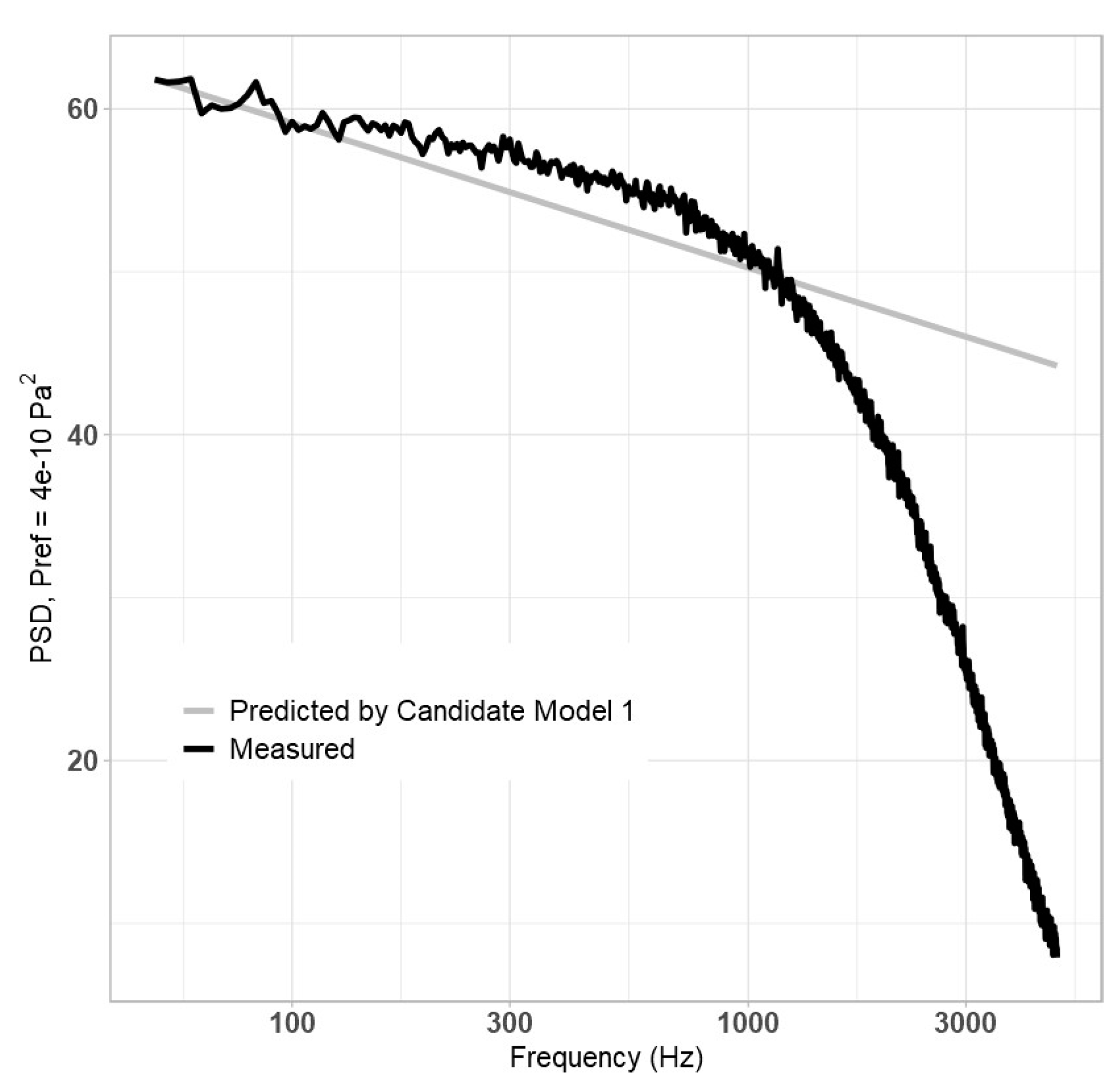
Table 4 later in this section. The resulting plot is shown in
Figure 1, below.
Clearly, Equation (16) is unable to adequately predict high-frequency behaviour and could benefit from improvement at predicting initial values in the low-frequency region. It was hypothesized that adding a large, non-dimensional parameter, such as a Reynolds number, to the denominator may improve high-frequency slope prediction, as shown in Equation (17):
For the Reynolds number,
Reτ,
ReT,
Reθ, and
Re were all considered (referred to as Candidate Models 2A, 2B, 2C, and 2D, respectively), while all pressure, speed, and distance values were also considered. Ultimately, the model performed best when
q,
Uτ,
δ, and
ReT were used (2B), in which case
A = 5.0679 × 10
−6,
b = 1.611, and
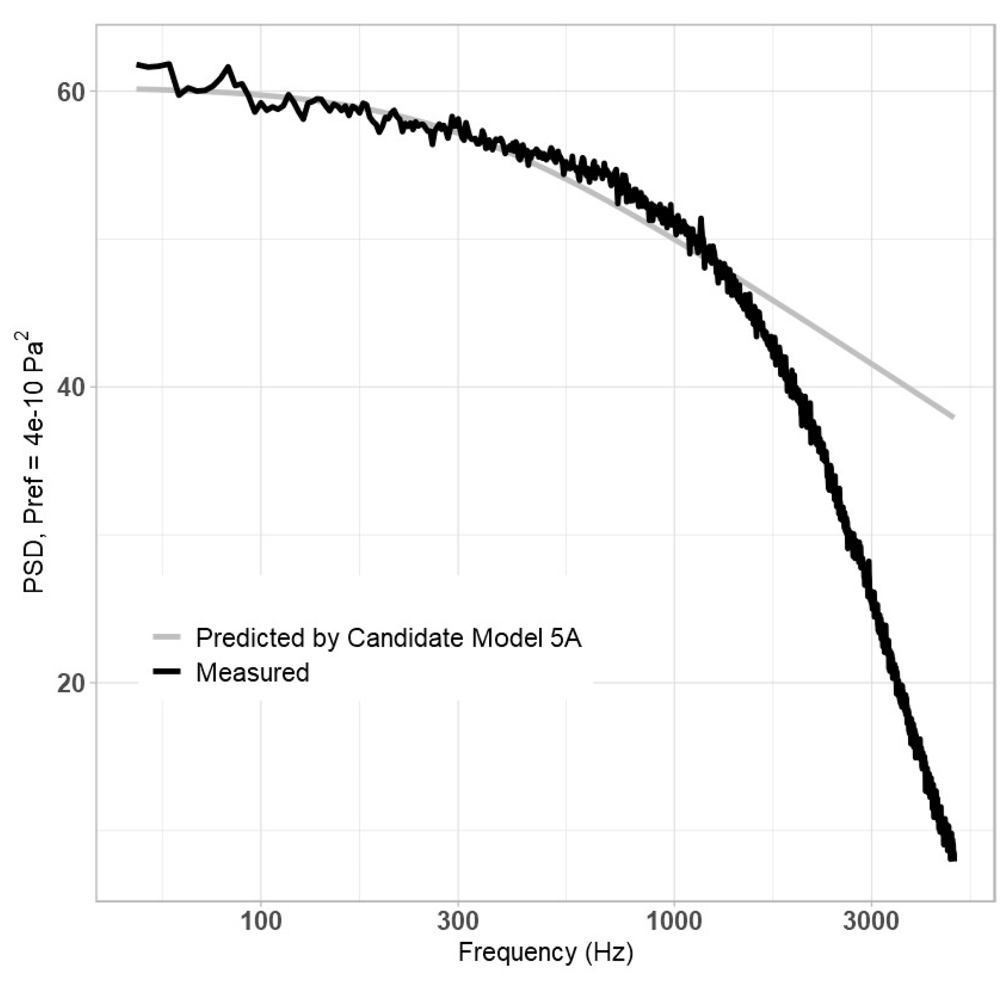
c = 0.60254. The resulting plot is shown in
Figure 2, below.
While Equation (17) did little to improve the high-frequency behaviour, it appeared to improve low-frequency behaviour. It was apparent by this point that the best way to predict the high frequency’s slope was by maximizing the exponent
b on the
St term. It was hypothesized that adding another non-dimensional parameter, either to the numerator (Equation (18a), Candidate Model 5A) or the denominator (Equation (18b), Candidate Model 5B), would free up the model to predict a higher value for exponent
b:
For the dimensionless parameter,
Cf,
M,
Re,
ReT,
Reτ,
Reθ,
Fr,
We, and
fv/
Uτ2 were considered, along with all terms from previous models. Ultimately, (18a) performed best when
q,
Uτ,
δ, and
ReT were used for the Reynolds number, and
Re was used for the dimensionless parameter. In this case,
A = 2.922 × 10
−15,
b = 2.657,
c = 1.4447, and
d = 1.7377. The resulting plot is shown in
Figure 3, below.
Equation (18a) demonstrated improvement over previous models, as it maintained accurate prediction of PSD for much longer into higher frequency regions; however, improvement was still required. By this point it had become evident that a high exponent b on St would be necessary to adequately model high-frequency behaviour, as aside from the Goody parameter, which was not compiled in the algorithm, no other candidate variables varied with frequency. As such, Equation (18a) was modified in two parts. First, in the high-frequency range, Equation (19) was fitted to the data:
Three definitions of “high frequency” were used:
f ≥ 500 Hz,
f ≥ 300 Hz, and
f ≥ 1000 Hz. At 500 Hz, the NLS algorithm predicted that
b = 4.1743; at 300 Hz,
b = 5.2179; and at 1000 Hz,
b = 3.6339. Next, keeping those exponents constant, Equation (18a) was re-fitted to create Candidate Models 6A, 6B, and 6C. As was the case before, all pressures, velocities, distances, Reynolds numbers, and non-dimensional parameters were reconsidered. The model performed best when
f ≥ 500 Hz (
b = 4.1743) was used, along with
q,
Uτ,
δ, and
ReT being used for the Reynolds number, and
Reθ was used as the non-dimensional parameter. The resulting equation (Candidate Model 6B) is shown as Equation (20), below:
In this case,
A = 7.2018 × 10
−5,
c = 2.3973, and
d = 2.4624. The resulting plot is shown in
Figure 4, below.
This model performs better in the high-frequency region than earlier models. Interestingly, it appears to perform slightly worse at low frequencies. It was theorized that the large exponent of St caused it to “dominate” behaviour at all frequencies, and thus, adding a small (much less than zero) coefficient to the St would allow the numerator to instead dominate early behaviour, as in Equation (21), Candidate Model 7, below:
This model was otherwise derived as Equation (20), with each of the three values for
b, along with all parameters, being reconsidered. The model performed best when
q was used for pressure,
Uτ was used for speed,
δ for distance,
ReT for the Reynolds number, and
M for the dimensionless parameter. The model performed similarly well when
b = 4.1743 (
f ≥ 500 Hz; Candidate Model 7A) and
b = 5.2179 (
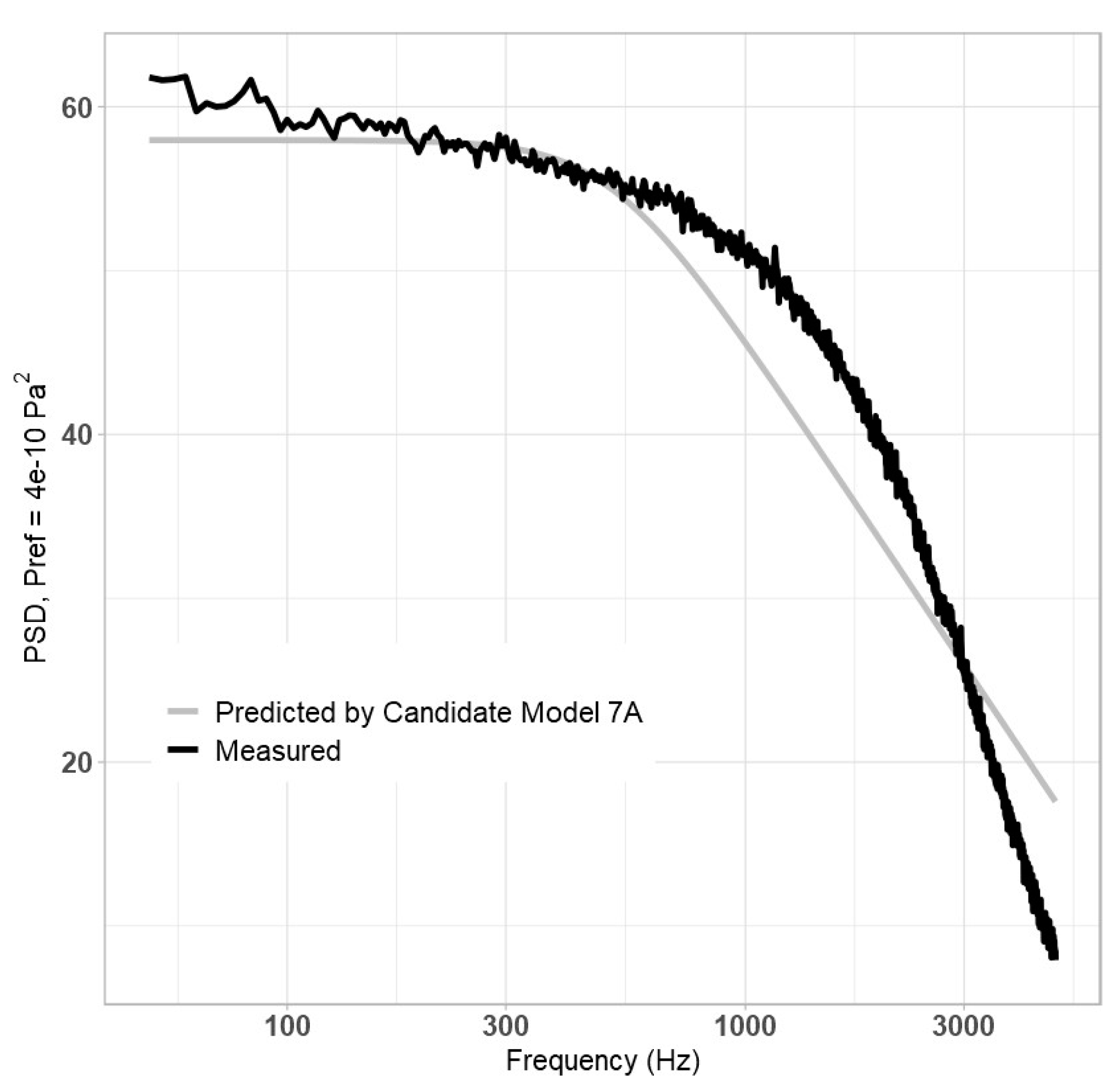
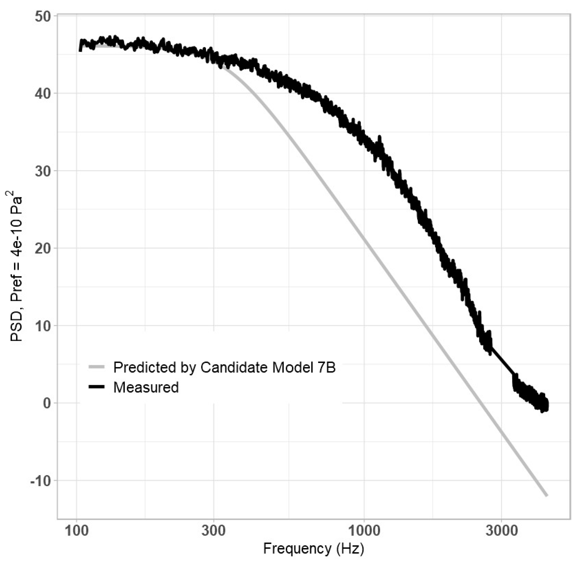
f ≥ 300 Hz; Candidate Model 7B). The results are shown in
Figure 5 and
Figure 6, below.
For the b = 4.1743 case, A = 0.39031, c = 1.3968, d = 2.6241, and E = 0.019972; for the b = 5.2179 case, A = 0.37047, c = 1.3697, d = 2.6574, and E = 0.0013168. As can be seen in the figures, improvement was minimal in comparison to Equation (20). Further attempts to modify the model either offered negligible performance improvements or could not compile due to limitations with the NLS algorithm.
The
MSPE,
AIC, and
BIC scores of each model are presented in
Table 4, below.
According to the MSPE statistical test, (21) performs best, particularly for Candidate Model 7B (when
b = 5.2179 is used), followed by the model generated from Equation (20). These models were particularly accurate at high frequencies, while earlier models were similarly accurate at lower frequencies. This distinction is important, given that a main practical application of this model would be to estimate passenger aircraft cabin noise levels—human ears are most sensitive to noises between 500 and 4000 Hz [
35]. Thus, a model that can adequately predict high-frequency PSD, but not low-frequency PSD, is more useful than a model that does the opposite. Since Equation (21), particularly the
b = 5.2179 case, best modeled high-frequency PSD, it was selected as the final model:
Next, the model validation step was performed (recall from
Section 2 that this involved comparing data performance against the testing data and outside data). Equation (22) showed a better agreement with the testing dataset—as depicted in
Figure 7, below—with the most notable inaccuracy being that the high frequency’s downslope starts too early.
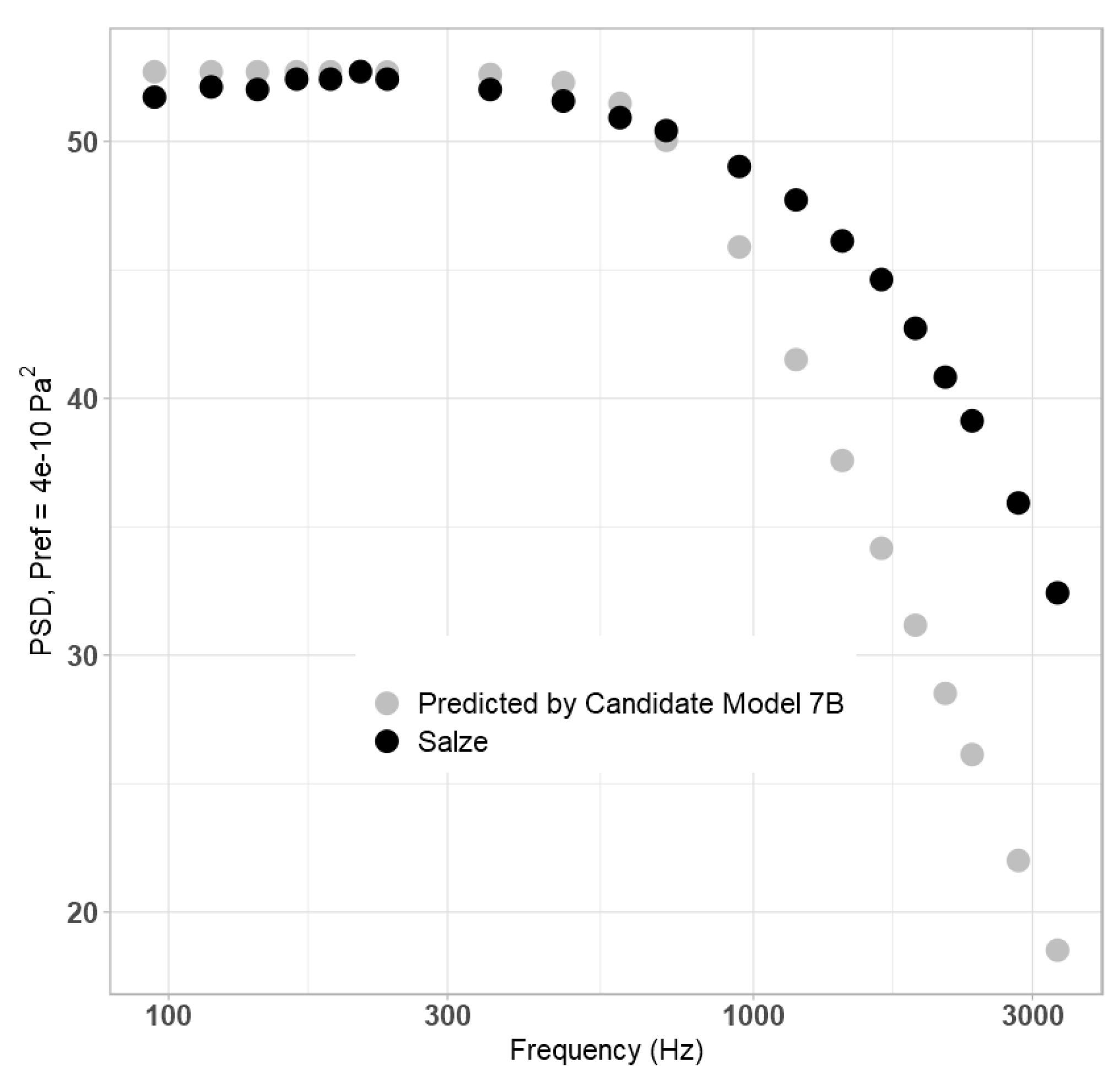
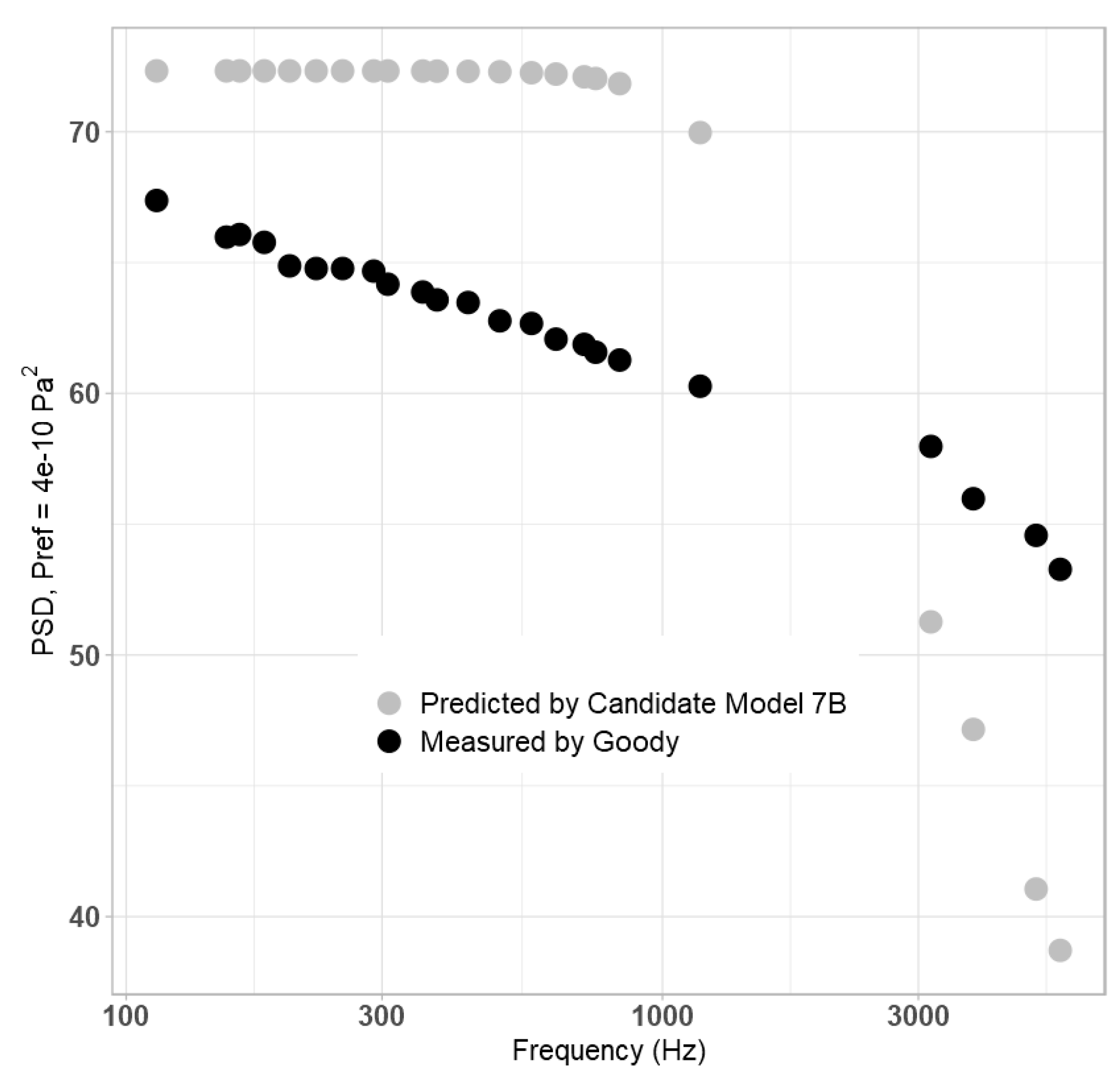
For the outside data, three datasets were considered: Gravante (Gravante2953w) [
36], which was at a higher Reynolds number and lower freestream velocity to the training/testing datasets; Salze (Salze1642w) [
37], which was comparable in both cases; and Goody (Goody7300w) [
38], which was at higher values for both. The values of frequency, PSD, and flow parameters (for example,
δ and
Re) were estimated and/or calculated at several key points by Thomson and Rocha, several of which are summarized in
Table 5, below. To ensure consistency from experiment to experiment, and to make up for missing data, Thomson and Rocha used only the listed Mach number, stream-wise location, pressure, and temperature from the original studies. All other values were calculated using consistent formulas (please refer to Appendix B in [
39] for more information). Thomson and Rocha reported more values than were present in the original studies [
39]. The values from Thomson and Rocha are reported in
Table 5.
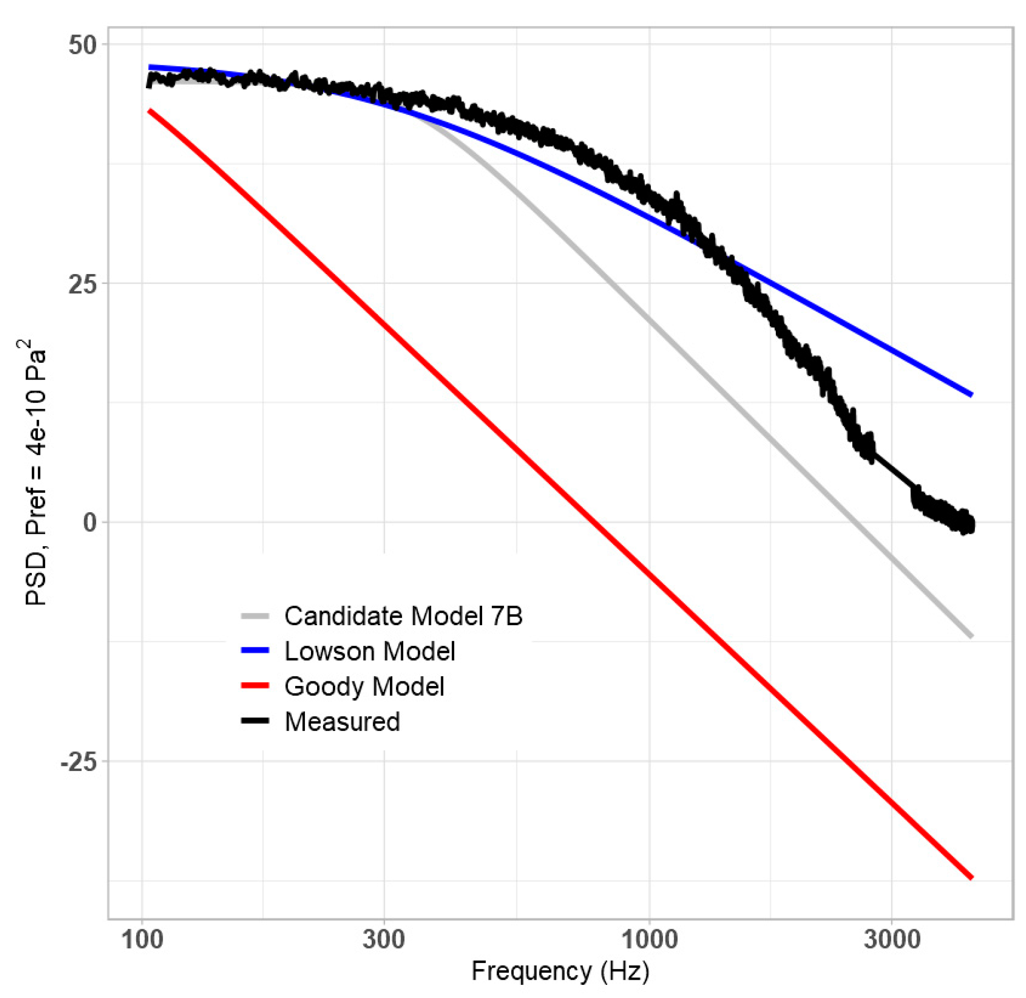
Additionally, a plot of the final model’s prediction of measured data (grey) vs. the predictions of the Lowson (blue) and Goody (red) models has been included in
Figure 11. The proposed final model provides the most accurate prediction of the three.
Based on these figures, the proposed model is accurate under its design conditions, along with the lower airspeed presented by the Gravante dataset, but is less accurate against the Goody dataset. It is theorized that this struggle is due to the lack of parameters that vary with frequency in the training dataset, as it effectively required the downslope to be entirely predicted by the St term, along with the relative lack of unique data conditions. This is problematic for two reasons: first, it is well documented in literature that the dependence of PSD on
St varies with frequency [
37,
38].
If more frequency-varying parameters were present, a model could be designed, for example, to have a very small coefficient but an exponent of −7.6 on
St, such that it dominates at high frequencies, but not at mid and low frequencies. However, practical limitations require the exponent to be smaller to, at minimum, accurately model the overlap region [
40,
41]. Similarly, the limited variation in training data does not permit the model to even consider the possibility of unique high-frequency behaviour, such as in the case of the Goody data, in which there is relatively little downslope.
However, beyond the accuracy, the method used in this paper presents several advantages and conclusions. First, its iterative nature allowed 186 different model forms to be tested and statistically assessed. This number is unmatched in the previous literature, except, perhaps, by the Dominique model. However, the black box nature of ANNs meant that the Dominique model did not provide the same level of insight into each case [
22]. A significant secondary advantage of generating 186 different model forms is that it allowed for a database consisting of all results to be published in [
42]. Future researchers should strongly consider incorporating any of these models into their research and analysis, as it is expected that certain alternative models will perform better at novel airspeed and turbulence conditions. Furthermore, as the model generation procedure did not rely on TBL-specific physics, it can be more broadly applied to other scientific and engineering applications. Even within the field of TBL-PSD modelling itself, future researchers may consider applying it to data cases not covered in this paper, such as adverse and favourable pressure gradients. Finally, the open nature of the procedure offers evidence answering several open-ended questions in TBL-PSD modelling. For example, this paper demonstrates that the most accurate models were generated when Re
T is the Reynolds number used in the denominator, and similar evidence that the optimum combination of variables to use in the velocity/time term is U
τ and δ.
