Minimum-Data-Driven Guidance for Impact Angle Control

Abstract

This paper investigates the impact-angle-control guidance problem for varying-speed flight vehicles with constrained acceleration. A learning-based bias proportional navigation guidance (L-BPN) law is proposed to achieve impact-angle-constrained impact by constructing a deep neural network (DNN) for nonlinear mapping between the impact angle and the bias term. During the process of dataset establishment, the impact of state variables is evaluated by sensitivity analysis to minimize the quantity of training data. This approach also effectively accelerates sample generation and improves the training efficiency. The simulation results verify the effectiveness of the proposed L-BPN law and demonstrate its advantages over the existing algorithms.

1. Introduction

Impact-angle-control guidance (IACG) [1,2,3] is an important flight vehicle guidance technology and is of great significance for improving the flight accuracy and effectiveness of a flight vehicle to cope with complex targets and environments as well as for enhancing the flexibility of guidance systems [4,5,6].

For IACG problems, trajectory-shaping guidance (TSG) [7,8] is commonly used. This method is based on optimal control theory and realizes impact angle control according to the time to go. Subsequent studies [9,10] have been improved on the basis of TSG, thereby solving problems such as extending to three-dimensional planes or adding bias terms, and solving constraints such as impact time. Subsequently, nonlinear control methods, such as sliding mode control [11,12,13], were also applied to IACG problems to design non-singular terminal guidance laws to effectively realize angle control. The above guidance laws to realize the precise control of the impact angle are inseparable from the current time to go, which can be obtained by making calculations according to the current distance. However, infrared, laser semi-active, and other guides cannot measure distance information directly, meaning that the time to go cannot be estimated. In view of the above problems, the application of the bias proportional navigation guidance (BPNG) law poses a wider range of difficulties than expected [14,15,16]. Among them, constant bias proportional navigation guidance (CBPNG) [17,18] adds impact angle constraint bias terms on the BPNG, which only needs the angle rate of the visual line of sight and the flight vehicle velocity information to realize the impact angle constraint. The guidance structure is simple, and it has the potential for certain applications in engineering. This study thus carries out research on the basis of this guidance law. However, the analytical solution that has been obtained assumes constant speed, and because speed varies in actual flight, the result does not reach the desired impact angle. Additionally, the acquisition of the bias term requires an integral operation that is large and time-consuming.

The analysis of the analytical solution formulas shows that there Is a strong nonlinear mapping relationship between the bias term and the terminal impact angle of the flight vehicle, and deep neural networks (DNNs) have been shown to be able to accurately respond to this type of mapping relationship with low computational effort [19,20,21,22]. Hypersonic vehicle re-entry multi-constraint guidance based on a predictive correction guidance framework, where the prediction module of the predictive correction is implemented by a DNN, is implemented in [19]. A functional relationship between the expression of the optimal guidance law and the relative state of the flight vehicle was established in [20] and achieved by training a DNN. Although the exact guidance equation cannot be obtained, it is possible to obtain the guidance law by training another DNN with a set of termination conditions. An online neural network guidance law that considers the randomness of perturbations during flight vehicle flight was designed in [21], allowing for online compensation once the perturbation appears. A model-based deep learning method was proposed in [22], where the structure of the guidance law was first obtained based on the model’s predictive control, and then a DNN was used to approximate the predictive model of the guidance dynamics and incorporate it into the model predictive path–integral control framework, enabling the designed guidance law to adapt to complex environments. Although DNNs are better suited to solving mapping relations in guidance control, the amount of training samples required is generally larger. The cost of obtaining data is also extremely high, and the minimum amount of data possible needs to be applied for training.

In order to solve the problems of the high cost of acquiring data and the large arithmetic volume of DNNs, this study proposes a minimum-data-based approach that uses the least amount of data possible while ensuring the accuracy of DNN training. In optimization theory, sensitivity analysis [23,24,25] can determine how changes in input parameters affect the output or performance of the system or model, providing the degree of influence of each parameter on the objective function or constraints. This helps to identify the parameters that have little effect on the system, thus reducing the data required for training. Based on the above theory, first, a mapping relationship between the bias terms and the flight vehicle state quantities is derived from the analysis of the analytical solution. Second, the sensitivity analysis of each state parameter is carried out, i.e., when observing a certain parameter, the rest of the states are fixed, and the degree of influence on the bias term is analyzed according to its change. According to the degree of influence of each parameter, the samples are established. That is, when the sensitivity is small, the sampling interval is large and the sample size is selected to be low, and vice versa. Based on this method, the amount of data can be minimized while also ensuring training accuracy.

The main contribution of this paper is twofold. Firstly, the amount of data required is minimized. A sensitivity analysis is performed on the state parameters to determine how much they affect the bias constants. This analysis helps to minimize the sample size on which the database is built. Secondly, the mapping relationship between the bias term and desired impact angle is derived and proved, which provides a theoretical basis for the application of the DNN.

The rest of this paper proceeds as follows: Section 2 discusses issues with traditional methods for calculating the bias constant and analyzes the disadvantages of the current methods for estimating the total flight time under varying-speed conditions. Section 3 demonstrates the nonlinear mapping relationship between the bias term and parameters and analyzes the sensitivity of each state variable to minimize the amount of data. In Section 4, we describe how the training of samples was carried out, followed by the numerical simulations in Section 5. Finally, Section 6 provides the conclusions.

2. Prerequisites and Background

2.1. Flight Dynamics

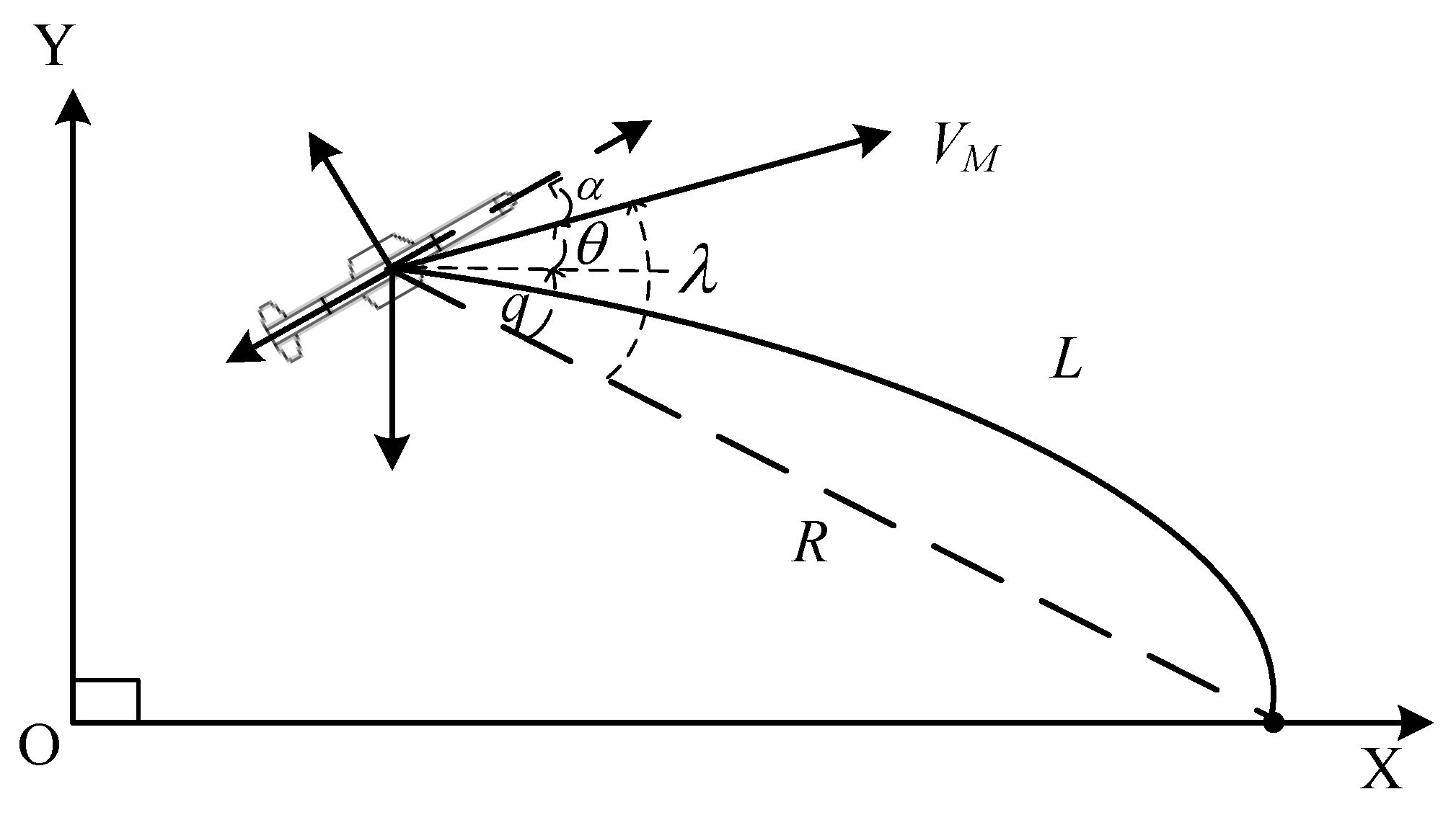
A flight vehicle maneuvers mainly in the vertical plane to regulate its range by gliding. The spatial guidance problem can generally be divided into two orthogonal planar cases with the well-known separation concept, and this paper mainly investigates the guidance problem in the vertical plane, as shown in Figure 1. The variables $\theta$, $q$, and $\lambda$ represent the flight path angle, line-of-sight (LOS) angle, and lead angle, respectively. The notation $R$ denotes the range, representing the length of the trajectory. And $V_M$ stands for the velocity. The drag, lift, and gravity forces imposed on the flight vehicle are denoted by $F_x$, $F_y$, and $F_G$, respectively.

The kinematic differential equations of the flight vehicle can be expressed as

$${\dot{V}}_M=\frac{-F_x-F_G\sin \theta }{m}$$

(1)

$$\dot{\theta }=\frac{a_M}{V_M}$$

(2)

$$\dot{R}=-V_M\cos \lambda$$

(3)

$$\dot{q}=-\frac{V_M\sin \lambda }{R}$$

(4)

where $a_M$ is the lateral acceleration command, and the aerodynamic forces imposed on the flight vehicle can be formulated as

$$F_x=C_{x}QS$$

(5)

$$F_y=C_{y}QS$$

(6)

$$F_G=mg$$

(7)

where $C_x$ and $C_y$ are for the lift and drag coefficients, respectively; $S$ is the reference area of the flight vehicle; $m$ is the mass of the flight vehicle; $g$ is gravitational acceleration; and $Q$ is the dynamic pressure, which is formulated as

$$Q=\frac{1}{2}\rho V_M^2$$

(8)

where $\rho$ is the air density, which can be obtained from [26]. The terminal constraints of the flight vehicle are

$$x(t_f)=x_T,y(t_f)=y_T$$

(9)

$$\theta (t_f)={\theta }_d$$

(10)

where ($x_T$, $y_T$) represents the target position, and ${\theta }_d$ is the desired impact angle. Hence, the guidance problem explored in this paper can be formulated as a finite-horizon problem governed by the differential Equations (1)–(4) with the terminal constraint Equations (9) and (10).

2.2. CBPNG Law Analysis

To satisfy Equation (9), the most widely applied guidance method currently is the PNG law, especially in engineering applications. As long as the flight vehicle’s seeker can measure the flight vehicle–target LOS angular rate, or the flight vehicle’s onboard equipment can calculate this angular rate based on the relative motion of the flight vehicle and the target, PNG can be used. The structure of PNG is simple, making it is easy to implement in engineering projects, and it is effective against stationary or slowly moving targets, for which its specific form is as follows:

$$a_N=V_{M}N\dot{q}$$

(11)

where $N$ is the proportional constant. However, traditional PNG cannot satisfy Equation (10); therefore, BPNG is proposed. The original intention is to add an angular control bias term to the basis of PNG, thereby achieving constraints on the impact angle. Among BPNG laws, CBPNG only requires the accurate calculation of the bias term constant to obtain the corresponding desired impact angle, which has the following form:

$$a_M=a_N+a_b=V_{M}N\dot{q}+V_{M}b$$

(12)

where $b$ is the constant bias term for impact angle control, and $a_b$ is the bias term, which can converge the terminal impact angle to the desired value. Integrating Equation (12) yields

$$\theta (t)-{\theta }_0=N(q(t)-q)+{\displaystyle {\int }_0^{t}bdt}$$

(13)

where ${\theta }_0$ is the initial flight path angle. When time $t$ becomes the terminal time $t_f$, Equation (13) becomes

$${\theta }_f={\theta }_0+N(q_f-q_0)+{\displaystyle {\int }_0^{t_f}bdt}$$

(14)

where $q_f$ is terminal LOS angle. For ground targets, when the terminal velocity direction points towards the LOS to the target ${\theta }_f=q_f$, by substituting into Equation (14), the terminal impact angle can be obtained as follows:

$${\theta }_f=\frac{N{q}_0-{\theta }_0-{\displaystyle {\int }_0^{t_f}bdt}}{N-1}$$

(15)

From Equation (15), if ${\displaystyle {\int }_0^{t_f}bdt}$ is accurately estimated, the solution for ${\theta }_f$ is analytical. We see that when the initial conditions are determined, ${\theta }_f$ can be achieved by adjusting the magnitude of ${\displaystyle {\int }_0^{t_f}bdt}$. If full-course CBPNG is used, we need to estimate the total flight time $t_f$. However, the traditional methods [27,28] cannot accurately estimate this, and they are only applicable under the assumption of constant velocity. Under varying-speed conditions, they are not able to achieve the desired impact angle. Clearly, from Equation (15), ${\displaystyle {\int }_0^{t_f}bdt}$ has a mapping relationship with other parameters. Furthermore, neural networks have the advantages of high solution accuracy and fast computation speed in dealing with mapping relationship problems; therefore, this paper proposes a learning-based method to accurately solve ${\displaystyle {\int }_0^{t_f}bdt}$.

3. Offline Database Building

In this section, the construction of samples required for neural network training is presented. First, we conduct a mapping analysis to provide theoretical support for obtaining samples through simulation. Second, we perform a sensitivity analysis, which can achieve sample reduction while ensuring accuracy, thereby reducing computational costs during training. Finally, we establish a sample database based on the above analyses.

3.1. Mapping Analysis

From Equation (15), the relationship between the constant bias term and the terminal impact angle can be expressed as

$$b=\frac{N{q}_0-{\theta }_0-(N-1){\theta }_f}{t_f-t_0}$$

(16)

and Equation (16) can be transformed into

$${\theta }_f=\frac{N{q}_0-{\theta }_0-(t_f-t_0)b}{N-1}$$

(17)

The errors in the above formulas are due to the small-angle assumption and the inaccurate estimation of the flight time, and compensation can be carried out by introducing deviation terms $\Delta \eta$ and $\Delta t$ for angles and time, respectively, to account for the actual correspondence. For computational convenience, we adopt the method of Equation (15) and incorporate $\Delta \eta$ and $\Delta t$:

$${\theta }_f=\frac{N{q}_0-{\theta }_0+\Delta \eta -\left(\frac{R_0}{V_{M0}}+\Delta t\right)b}{N-1}$$

(18)

where $R_0$ and $V_{M0}$ are the initial distance and flight vehicle velocity, respectively. In Equation (18), the initial parameters such as $N$, $q_0$, ${\theta }_0$, $R_0$, and $V_{M0}$ are known and treated as constants, i.e., fixed values. ${\theta }_f$ is typically taken as a negative value, such that Equation (18) becomes the following:

$$|{\theta }_f|=\frac{\left(\frac{R_0}{V_{M0}}+\Delta t\right)b-N{q}_0-{\theta }_0+\Delta \eta }{N-1}$$

(19)

Even though the specific values of $\Delta \eta$ and $\Delta t$ are unknown, they do not affect the signs of the parameters. Therefore, the numerator term $\left(R_0/V_{M0}+\Delta t\right)b-N{q}_0-{\theta }_0+\Delta \eta$ is positive. From Equation (19), we infer that $\left|{\theta }_f\right|$ is a strictly monotonic increasing function with respect to $b$. Exactly monotonic functions have one-to-one mapping relationships. Therefore, when the other initial parameters in Equation (19) are given, we can prove that $\left|{\theta }_f\right|$ and $b$ have a one-to-one mapping relationship. The relationship between $\left|{\theta }_f\right|$ and $b$ can be expressed as follows:

$${\theta }_f=f(R_0,V_{M0},N,q_0,{\theta }_0,b)$$

(20)

Theorem 1.

Let $y=f(x)$, where $x\in D$ is strictly increasing or decreasing. Then, function $f$ must have an inverse function $f^{-1}$, which is also a purely monotonic function with respect to $f(x)$ within its domain.

Proof of Theorem 1.

Since f is strictly increasing over $D$, for any $y\in f(D)$, there exists an $x\in D$ such that $f(x)=y$.

Assume $c=d$, where $d$ is strictly increasing. Let $y\in f(D)$, and show that there exists $x\in D$ such that $f(x)=y$

Since $y\in f(D)$, there exists some $x’\in D$ such that $f(x’)=y$. Since $f$ is strictly increasing, for any $x>x’$, $f(x)>f(x’)$. Similarly, for any $x<x’$, $f(x)<f(x’)$.

Consider the case where $d=x’$. Since $c=d$, $f(c)=f(d)=y$. Thus, $x=c=d$ such that $f(x)=y$.

Now, consider the case where $d>x’$. Since $d$ is strictly increasing, $c<d$ and $f(c)=y$. Since $f$ is strictly increasing, for any $x>d$, $f(x)>f(d)=y$. Similarly, for any $x<c$, $f(x)<f(c)=y$. Thus, there is an $x$ such that $c<x<d$ and $f(x)=y$.

Consider the case where $d<x’$. Since $d$ is strictly increasing, there exists some a such that $c>d$ and $f(c)=y$. Similarly, for any $x<d$, $f(x)<f(d)=y$. Thus, there is an $x$ such that $d<x<c$ and $f(x)=y$.

In all cases, for any $y\in f(D)$, an $x\in D$ such that $f(x)=y$ exists. Therefore, function f is inverse, and it is a strictly monotonic function with respect to $d$ within its domain. This completes the proof of Theorem 1. □

According to Theorem 1, the inverse function of Equation (20) is also strictly increasing. Therefore, a one-to-one mapping relationship exists between $\left|{\theta }_f\right|$ and $b$, as shown below:

$$b=f^{-1}(R_0,V_{M0},N,q_0,{\theta }_0,{\theta }_f)$$

(21)

Equations (20) and (21) can be approximated as inverse transformations. In ideal conditions, the inversion is exact. However, inversion errors may occur in the inverse process because of approximation transformations or parameter changes. A neural network can be used to represent this nonlinear inverse transformation. During offline training, an accurate mathematical model can provide an approximate inversion that adapts to the total flight envelope. This allows the neural network to compensate for the inversion errors online.

For R and $q_0$ in Equation (20), according to the trigonometric relationship, we replace them in the form of $x_0$ and $y_0$. This has the advantage of reducing the amount of calculation. The coordinate information of the flight vehicle is directly available, while R and $q_0$ need to be calculated. Additionally, based on the analysis in the previous section, limited acceleration has a significant impact on the impact angle. Hence, the mapping relationship between $\left|{\theta }_f\right|$ and b can be transformed as follows:

$$b=f^{-1}(x_0,y_0,V_{M0},N,a_{\max },{\theta }_0,{\theta }_f)$$

(22)

Subsequently, Equation (22) represents the mapping relationship in this paper, replacing Equation (21). Suppose all data from each dimension in the input are used as a sample. In that case, this approach results in many samples, significantly increasing computational complexity. Moreover, each dimension may have a different influence on $b$. Therefore, conducting sensitivity analysis on each dimension, selecting appropriate sample intervals, and employing different sampling strategies can help reduce the computational burden while maintaining accuracy.

Sensitivity analysis performed on each dimension identifies those that significantly impact the mapping relationship. A smaller sample interval is selected for these dimensions to capture variations more accurately. Conversely, a larger sample interval is chosen for dimensions with a relatively minor impact, reducing the number of samples without sacrificing accuracy significantly. These strategies effectively reduce the overall sample count while capturing an accurate mapping relationship between the input dimensions and $b$.

3.2. Sensitivity Analysis

In optimization theory, sensitivity analysis is often used to study the stability of the optimal solution when the original data are inaccurate or changes occur. The influence of parameters on the system or model can be quantified by conducting this sensitivity analysis, which helps explain how changes in input parameters affect the output or performance of the system or model. It provides insights into which parameters significantly impact the objective function or constraints and to what extent. This information is valuable for decision making, model validation, and robustness analysis. By evaluating the sensitivity of the system or model to parameter variations, we can identify critical parameters that require accurate estimation or control. Sensitivity analysis also helps identify parameters with little influence on the system, enabling simplifications or reducing the computational burden.

This subsection mainly analyzes the sensitivity of the constant bias term to variations in the parameters for sample reduction in Equation (22). To do this, Equation (22) is adjusted with respect to the parameters, resulting in the following:

$$\dot{b}={\dot{f}}^{-1}(x_0,y_0,V_{M0},N,a_{\max },{\theta }_0,{\theta }_f)$$

(23)

Based on the analysis in the previous section, a mapping relationship exists between $b$ and the parameters, indicating a functional relationship. Therefore, Equation (23) can be expanded as follows:

$$\partial b=\frac{\partial b}{\partial x_0}\frac{\partial x_0}{\partial t}+\frac{\partial b}{\partial y_0}\frac{\partial y_0}{\partial t}+\frac{\partial b}{\partial V_{m0}}\frac{\partial V_{m0}}{\partial t}+\frac{\partial b}{\partial N}\frac{\partial N}{\partial t}+\frac{\partial b}{\partial a_{\max }}\frac{\partial a_{\max }}{\partial t}+\frac{\partial b}{\partial {\theta }_0}\frac{\partial {\theta }_0}{\partial t}+\frac{\partial b}{\partial {\theta }_f}\frac{\partial {\theta }_f}{\partial t}$$

(24)

In Equation (23), the partial derivatives of the $x_0,y_0,V_{M0},N,a_{\max },{\theta }_0$ terms can be obtained through numerical integration methods. According to Equation (19), the partial derivatives of the ${\theta }_f$ term involve unknown parameters such as $\Delta \eta$ and $\Delta t$, making an analytical solution to Equation (24) challenging. Simulation-based validation can be used to assess the impact of variations in each parameter on $b$. By conducting simulations with different parameter values and observing the resulting changes in $b$, the sensitivity and magnitude of each parameter’s influence on $b$ can be determined. This empirical analysis can thus provide valuable insights into the relationship between the parameters and $b$.

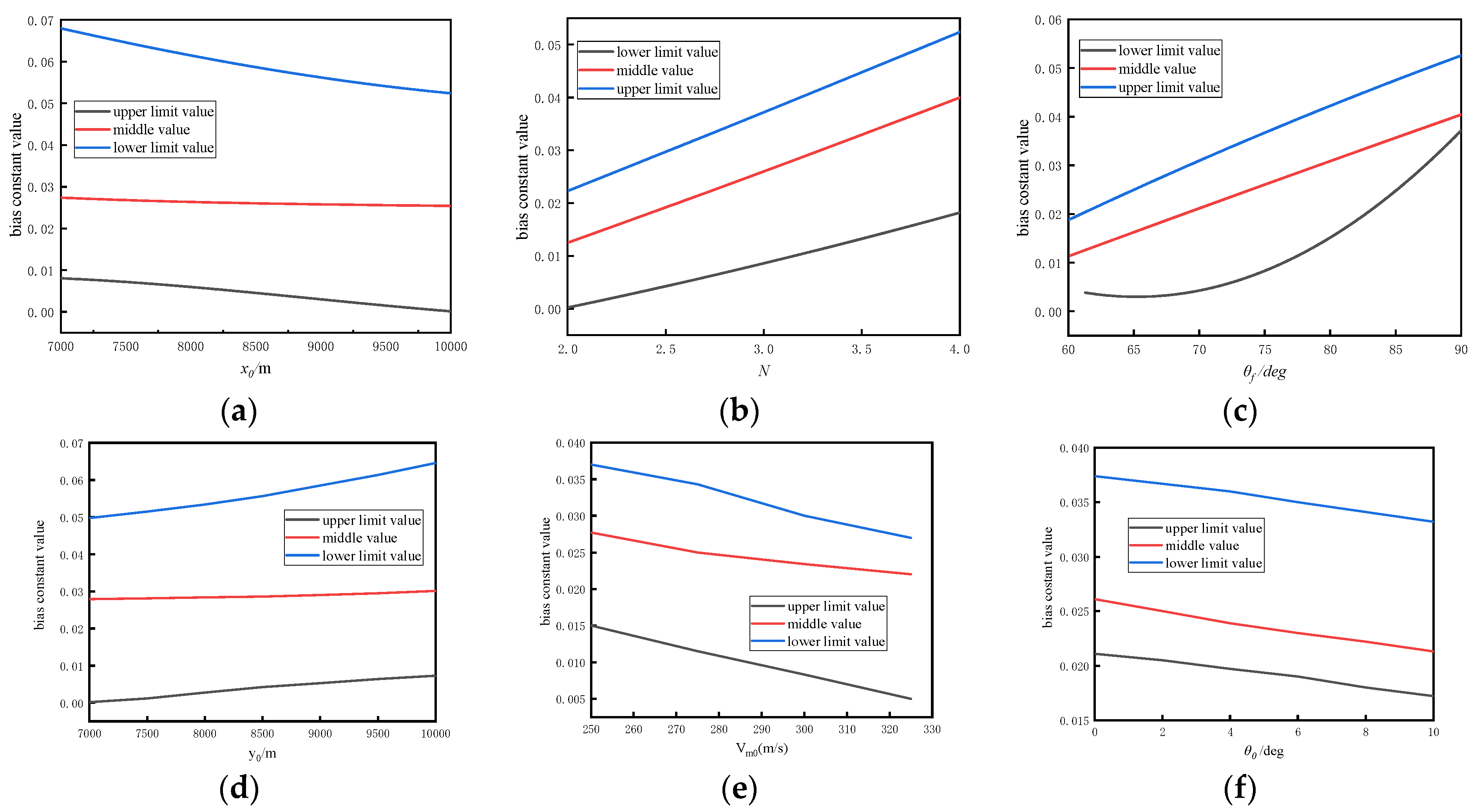
To establish a database and provide the boundaries for each dimension in Equation (22), such as $x_0\in \left(-\mathrm{10,000},-7000\right)m$, $y_0\in \left(7000,\mathrm{10,000}\right)m$, $V_{m0}\in \left(250,350\right)m/s$, $N\in (2,4)$, $a_{max}\in (2,4)g$, ${\theta }_0\in (0,10)deg$, and ${\theta }_f\in (-60,-90)deg$, we performed sensitivity analysis on each parameter on three levels: upper limit, middle value, and lower limit, which encompass the variations in all parameters and capture their trends.

First, when analyzing $x_0$ and $y_0$, since both represent the influence on distance, we only need to explore one. We define the three levels as $f^{-1}(x_1)$, $f^{-1}(x_2)$, and $f^{-1}(x_3)$, with parameter values of $(300, 2, 20, 0,-60)$ for the lower limit,$(300, 3, 30, 0,-75)$ for the middle value, and $(300, 4, 40, 0,-90)$ for the upper limit. Simulations were conducted for these three cases, and the results are shown in Figure 2a.

Based on the figure, whether considering the lower limit, middle value, or upper limit, the variation in $x_0$ has a relatively small impact on $b$, i.e., a low sensitivity. However, an overall decreasing trend is present. Therefore, when $x_0$ has smaller values, a larger sample interval should be chosen. On the other hand, when $x_0$ has larger values, a smaller sample interval should be selected.

Secondly, when analyzing $N$, we designated the three levels as $f^{-1}(N_1)$, $f^{-1}(N_2)$, and $f^{-1}(N_3)$, with parameter values of $(7000, 300,20,0,-60)$ for the lower limit, $(8500, 300,30,0,-75)$ for the middle value, and $(\mathrm{10,000}, 300,40,0,-90)$ for the upper limit. The results of the simulations for these three cases are shown in Figure 2b.

Based on the figure, in consideration of the lower limit, middle value, and upper limit, the variation in $N$ has a relatively significant impact on the value of $b$, and an overall increasing trend is present. Therefore, a smaller sample interval should be chosen, especially when $N$ is larger.

Finally, when analyzing ${\theta }_f$ for ease of analysis, we select $\left|{\theta }_f\right|$ as the analysis value. We designate the three levels as $f^{-1}({\theta }_{f1})$, $f^{-1}({\theta }_{f2})$, and $f^{-1}({\theta }_{f3})$, with parameter values of $(7000, 300, 2, 20, 0)$ for the lower limit, $(8500, 300, 3, 30, 0)$ for the middle value, and $(\mathrm{10,000}, 300, 4, 40, 0)$ for the upper limit. Simulations will be conducted for these three cases, and the results are shown in Figure 2c. The results show that regardless of the level considered, the variation in ${\theta }_f$ had a relatively significant impact on $b$, exhibiting an overall increasing trend. Therefore, a smaller sample interval should be chosen, especially when ${\theta }_f$ is larger. Additionally, from the lower limit curve, because, at larger desired impact angles, the acceleration capacity is limited, there is a slower response to the impact angle term and a steep increase in $b$. Hence, this experiment demonstrates the strong correlation between the desired impact angle term and acceleration capacity. Analyzing the limited acceleration and incorporating it as an input is crucial for accurate guidance.

For parameters such as $V_{m0}$ and ${\theta }_0$, the analysis methods are similar to those mentioned above, so these analyses are omitted. Furthermore, $a_{max}$ is already analyzed through the impact angle, resulting in the recommendation of a smaller sample interval. The analyses presented above provide a basis for establishing a strategy of evenly distributed sampling.

For sensitivity analysis, we mainly analyze its sensitivity level, because parameters with higher sensitivity have a greater impact on the output. At this point, the step size refers to the sampling step size, which is significantly different from the step size in general programs. Alternatively, it is more appropriate to use more sampling points for those that have a greater impact on the output and require more sampling points to ensure its accuracy. For those that have a smaller impact on the output, fewer sampling points can be used.

3.3. Sample Establishment

According to Equation (22), we consider different values for parameters as inputs for the samples. After training the neural network, $b$ is obtained for each state. The sample input form is as follows:

$$n_i=(n_i^{x_0},n_i^{y_0},n_i^{V_{m0}},n_i^N,n_i^{a_{\max }},n_i^{{\theta }_0},n_i^{{\theta }_f})\begin{array}{cc}& i=1,2,\dots n\end{array}$$

(25)

where $n_i$ represents the input vector at the $i$th time step, with the superscripts corresponding to the above-mentioned input quantities, and $n$ denotes the number of input steps.

Based on the analysis results from the previous section and to maintain accuracy while reducing the training sample size and saving training time, we reclassified the sampling interval. We sample $x_0$ and $y_0$ within the range of 7000–8500 m with a step size of 200 m and within the range of 8500–10,000 m with a step size of 200 m. In addition, $V_{m0}$ is sampled with a step size of 10 m/s; $N$ is chosen as 2, 3, and 4; $a_{max}$ is tested with a step size of 0.1 g; ${\theta }_0$ is sampled with a step size of 1°; and ${\theta }_f$ is sampled with a step size of 0.5°.

4. Offline Database Training

Based on the analysis in the previous section, different state parameters have varying effects on the bias term value. Their degrees of influence were examined, providing a reference for establishing samples in the next stage of the work. In the following section, we outline how a DNN was applied for training. Its overall architecture is analyzed and discussed, taking into account the boundedness of $b$. Our approach further demonstrates the stability of the guidance law, even with the bias term constant obtained by training the neural network.

4.1. Database Training

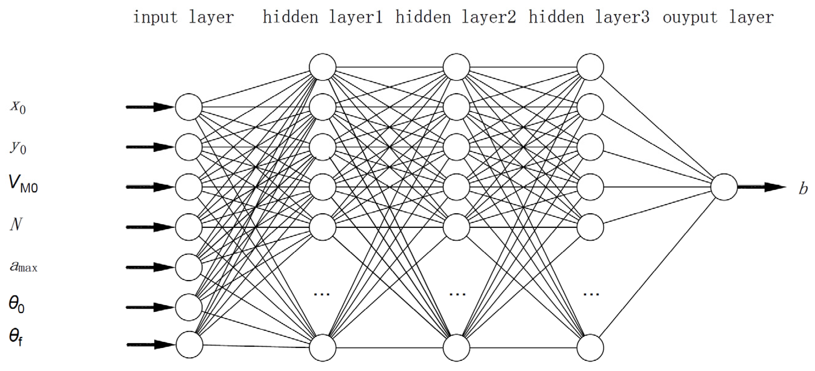
Neural networks are powerful mathematical models with strong nonlinear fitting capabilities. They can solve problems with which traditional reasoning models may struggle. By extracting, learning, and training on hidden patterns within training data and adjusting the weights of each node, neural networks can output values that tend to match those that are desired. Equation (22) indicates that the action is mathematically dependent on the current state and not on past moments. Therefore, this study applied a DNN to train the samples and learn the optimal state action relationships from the generated data. A DNN architecture [29] was designed with different layers and neurons per layer. Specifically, it comprised an input layer, an output layer, and three fully connected hidden layers, with each layer consisting of 20 neurons. The structure of the DNN is shown in Figure 3.

Data transfer between two layers is achieved through weighted connections. The mathematical model for the neurons used in this architecture is as follows:

$$\sigma =f\left({\displaystyle \sum _{i=1}^n{d}_i{\omega }_i+\delta }\right)$$

(26)

where $d_i$ is the input to the neuron; ${\omega }_i$ and $\delta$ are the weights and thresholds, respectively, of the corresponding neuron; $f(·)$ represents the activation function; and $\sigma$ denotes the output of the neuron. The rectified linear unit (ReLU) is the activation function for the input layer and hidden layers:

$$f(d)=\max (0,d)$$

(27)

In this study, we choose the minimum mean square error as the loss function. This involves computing the average squared difference between the desired output data and the actual output data:

$$E\left(\sigma ,\widehat{\sigma }\right)=\frac{{\displaystyle {\sum }_{i=1}^n{\left(\sigma -\widehat{\sigma }\right)}^2}}{n}$$

(28)

where $\widehat{\sigma }$ represents the bias term constant. The error obtained by subtracting the actual output data from the bias term constant data is propagated through the DNN. All network training continues until convergence using stochastic gradient descent. During the training process, error propagation is required if the error exceeds a predefined threshold. Taking the parameter ${\omega }_{hj}$ as an example for the backpropagation update process, given the error $E_k$ and learning rate $\eta$, the update $\mathsf{\Delta }{\omega }_{hj}$ equation is as follows:

$$\mathsf{\Delta }{\omega }_{hj}=-\eta \frac{\partial E_k}{\partial {\omega }_{hj}}$$

(29)

For Equation (29), according to the chain rule,

$$\frac{\partial E_k}{\partial {\omega }_{hj}}=\frac{\partial E_k}{\partial {\widehat{\sigma }}_j^k}\cdot \frac{\partial {\widehat{\sigma }}_j^k}{\partial {\beta }_j}\cdot \frac{\partial {\beta }_j}{\partial {\omega }_{hj}}$$

(30)

where ${\beta }_j$ is ${\displaystyle \sum _{i=1}^q{x}_h{\omega }_{hj}}$, and k is the number of neurons in the hidden layer. Parameter ${\omega }_{hj}$ can be updated as follows:

$${\omega }_{hj+1}={\omega }_{hj}-\eta \times \frac{\partial E_k}{\partial {\omega }_{hj}}$$

(31)

The training process of the DNN involves the continuous optimization of the network parameters through the backpropagation above and gradient descent algorithms to minimize the sum of squared errors. When the error reaches the desired level, Equation (31) is no longer updated, and the training is completed. The learning rate in Equation (29) remains constant, resulting in slow convergence. Therefore, in this study, we utilize the Adam learning method, which enables adaptive learning rate adjustment, to accelerate network convergence. The optimized parameters are denoted as follows:

$$E{\left(\sigma ,\widehat{\sigma }\right)}_{new}=E{\left(\sigma ,\widehat{\sigma }\right)}_{old}-\eta \nabla E\left(\sigma ,\widehat{\sigma }\right)$$

(32)

Since the learning rate in Equations (29) and (32) is an initial preset value used for training, the Adam optimizer [30] adaptively adjusts this parameter during the DNN training.

4.2. Overall Architecture and Boundedness of the Constant Bias Term

A neural network’s structure, scale, computational complexity, and solution accuracy are closely related. Accordingly, based on the sample sampling strategy derived from sensitivity analysis in the previous section, mathematical simulations are performed to generate batches of samples. After training, the DNN can be used online. The technical architecture of this study is illustrated in Figure 4.

We now discuss the boundaries of the bias term $b$. For the last layer of the neural network,

$$\begin{array}{l}h=f\left(\omega \cdot x+c\right)\\ o=\omega \cdot h+c\end{array}$$

(33)

where $\omega$ and $c$ represent the weights and biases of the neurons, respectively, and $o$ is the output value. Equation (33) can be written in a norm form as follows:

$$\Vert o\Vert =\Vert \omega \cdot h+c\Vert$$

(34)

The right-hand side of the equation can be further bounded using the triangle inequality for norms:

$$\Vert \omega \cdot h+c\Vert \le \Vert \omega \cdot h\Vert +\Vert c\Vert$$

(35)

For the input $h$ of the last layer of the neural network, which is the previous layer’s output, the activation function used in this paper is the ReLU function, with a range of $[0,1)$. Consequently, $\Vert \omega \cdot h\Vert \le \Vert \omega \Vert$, and the equation can be rewritten as follows:

$$\Vert \omega \cdot h+c\Vert \le \Vert \omega \Vert +\Vert c\Vert$$

(36)

According to the properties of the neural network, the values in $\omega$ and $c$ are network parameters. As long as the trained network parameters are bounded, according to Equation (36), the neural network’s output, i.e., the bias term $b$, is also determined. As such, the guidance law is considered stable. Therefore, after training the neural network, stability testing on the network parameters is needed. In this study, the weight of the last layer satisfies $\left|\right|\omega \left|\right|\le 10$ and $\left|\right|c\left|\right|\le 10$.

5. Simulations Results

In this study, we select a flight vehicle model. The reference area of the flight vehicle is S = 0.05 m² and the mass m is 100 kg. The gravitational acceleration g is assumed to be 9.81 m/s² and the navigation coefficient N = 3. The control input is chosen as the balanced angle of attack, $\alpha$. Since $\alpha$ is a small variable, the aerodynamic coefficients can be approximated as

$$\{\begin{array}{l}{C}_x=C_x^0+C_x^{{\alpha }^2}{\alpha }^2\\ C_y=C_y^{\alpha }\alpha \end{array}$$

(37)

where $C_x^0$ denotes the coefficient of parasite drag, and the coefficients with superscripts, $\alpha$ and ${\alpha }^2$, indicate the first- and second-order derivatives with respect to $\alpha$, respectively. The relationship between $\alpha$ and the guidance command is as follows:

$$\alpha =m{a}_M/(C_y^{\alpha }QS)$$

(38)

The control of the acceleration command can be converted into the control of $\alpha$ based on the above formula. The basic aerodynamic coefficients used in this study are shown in

Table 1. Basic aerodynamic coefficients.

Mach	${\mathit{C}}_{\mathit{x}}^0$	${\mathit{C}}_{\mathit{x}}^{\mathit{\alpha }}/\mathit{r}\mathit{a}{\mathit{d}}^{-1}$	${\mathit{C}}_{\mathit{y}}^{\mathit{\alpha }}/\mathit{r}\mathit{a}{\mathit{d}}^{-2}$
0.4	0.414	33.20	35.16
0.6	0.417	33.55	35.32
0.8	0.421	34.68	36.32
0.9	0.429	35.16	37.56

.

The subsequent simulations in this study use the above-mentioned flight vehicle coefficients. The simulation verification consists of five parts. In the first part, the fitting accuracy of the DNN is validated. The second part focuses on validating the model’s accuracy using a set of experimental data for simulation. The third part involves conducting Monte Carlo simulation experiments. In the fourth part, we compare the proposed method with traditional methods for calculating the total flight time. Finally, we examine the model’s robustness when considering the guidance system’s uncertainty.

5.1. Minimum-Data-Driven and Data-Driven Comparative Simulation

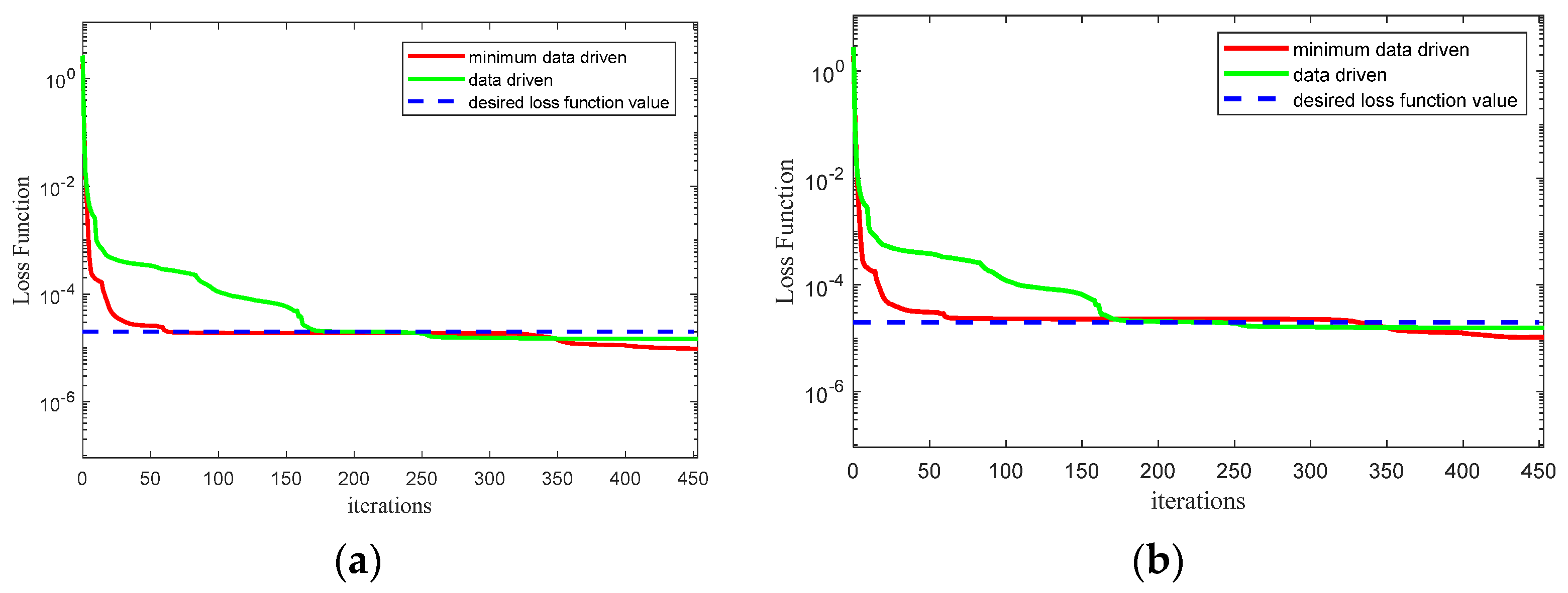
In this study, we utilized TensorFlow-2.12.0 to build the neural network model. Adam optimization was employed as the training algorithm, with a learning rate of 0.001. The hardware used for training included an Intel i5-12600k CPU and an NVIDIA RTX 3060ti 6G graphics card. The neural network model consisted of seven inputs and one output. It contained three hidden layers, each composed of 50 neurons. The simulation results were divided into training and testing sets, and the data were normalized. Based on the range specified in Section 2.2 and the sensitivity analysis of the parameters, 13,000 trajectories were collected. Among these, 12,500 trajectories were used for training, and 500 trajectories were used for testing. The two cases are compared by training set and test set, respectively. The results are shown in Figure 5 and

Table 2. The value of mean square error.

Data Processing Methods	Training Set	Test Set
Data-driven	0.0177	0.0083
Minimum-data-driven	0.0092	0.0116

.

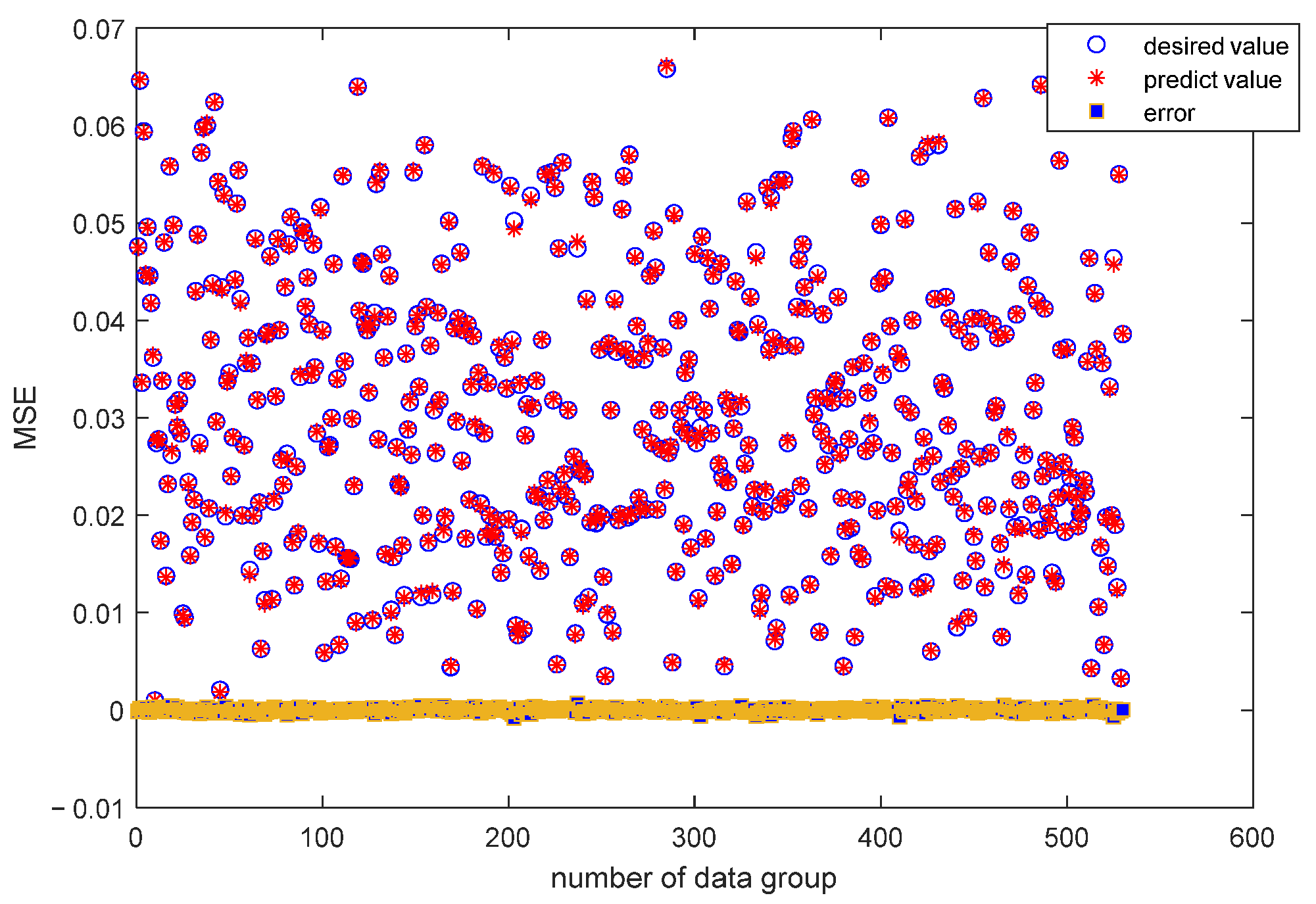
Set the loss function to 0.00001 or stop training when the number of iterations reaches 5000. As shown in Figure 1 and Table 1, there is a significant decrease in the loss function of the minimum data in the 52nd generation, which means that convergence has already begun since the 52nd generation. For those without data processing, convergence only begins in the 159th generation, indicating that the convergence speed is accelerated after minimum data processing. At the same time, training stopped in the 453rd generation after minimizing data processing, while training stopped in the 1172nd generation without minimizing data processing. The reason is that there is a large amount of data without data processing, resulting in overfitting. Whether it is the training set or the test set, the loss function values of the two are almost the same, both around 0.01, which proves that minimizing the amount of data processing also ensures training accuracy. Therefore, it can be further demonstrated that the data after minimization not only ensure training accuracy but also accelerate training speed, reduce training volume, and thus reduce training costs. The trained neural network was tested using 500 trajectories from the test set, and the predicted bias constant is shown in Figure 6.

Figure 6 shows that the predicted bias term values from the model are close to the actual values. The absolute error is 0.0014, and the mean squared error is 0.0034. This indicates that the trained model can achieve the desired impact angle.

5.2. DNN Model Accuracy

In this section, the accuracy of the trained model is validated. Three different initial conditions are selected for simulation. For ease of analysis, we set the initial velocity to $300 \mathrm{m}/\mathrm{s}$ and the target coordinates to $(0,0)$. The remaining simulation parameters are shown in

Table 3. Initial flight vehicle conditions.

Initial Flight Vehicle Position/m	Navigation Gain	Maximum Acceleration (m/s2)	Initial Flight Path Angle/°	Desired Impact Angle/°
(−10,000, 10,000)	3	20	0	−60
(−7000, 7000)	2	30	0	−70
(−8500, 8500)	4	40	0	−90

. The simulation results are shown in Figure 7.

The miss distance and actual impact angle for the three scenarios are shown in

Table 4. Miss distance and impact angle.

Scenario	Miss Distance/m	Impact Angle/°
1	0.06	−60.12
2	0.05	−69.80
3	0.26	−89.84

.

Figure 7 and Table 4 show that all three scenarios hit the target, and the difference between the actual impact angle and the desired impact angle is within $0.2°$. This indicates that the DNN model designed in this study has a high level of accuracy.

5.3. Monte Carlo Simulation

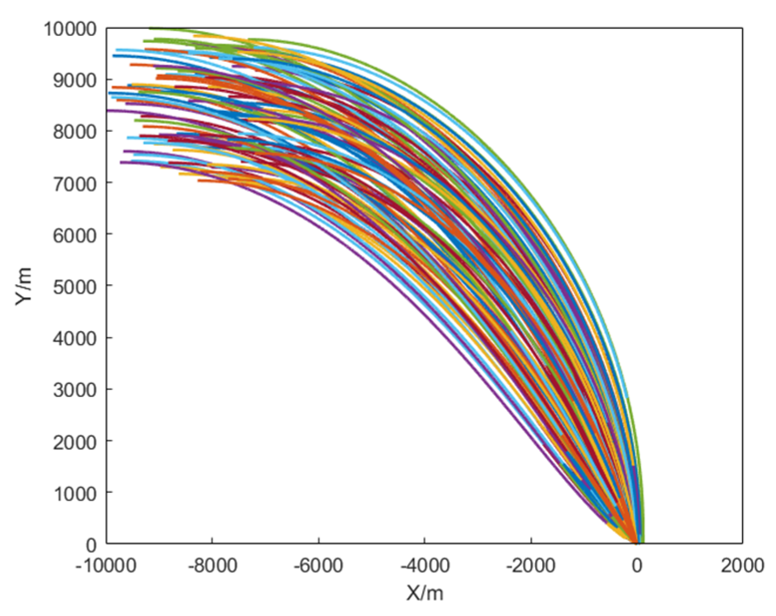
Monte Carlo simulation experiments were conducted to validate the DNN’s accuracy further. For illustration purposes, we randomly selected 100 sets of initial positions within the range of $(-7000, 7000)$ to $(-\mathrm{10,000}, \mathrm{10,000})$ and desired descent angles ranging from −60° to −90° while keeping the other parameters constant. The remaining parameters were set as follows: an initial velocity of 300m/s, target coordinates at $(0,0)$, an initial pitch angle ${\theta }_0$ of $0°$, a navigation gain $N$ of $2$, and maximum acceleration of 2 g. The flight vehicle’s trajectory for the randomly selected 100 sets of initial positions is shown in Figure 8, which shows that all 100 Monte Carlo simulation experiments resulted in hitting the target. The difference between the actual impact angle and the desired impact angle is shown in Figure 9.

Figure 9 shows that the minimum error in the desired impact angle is $0.02°$, the maximum error is $0.94°$, and the variance is $0.0833°$. The maximum relative error is less than $0.1\%$. Therefore, the DNN model designed in this study has low error, meeting the requirements for the desired impact angle.

5.4. Simulation Comparative Verification

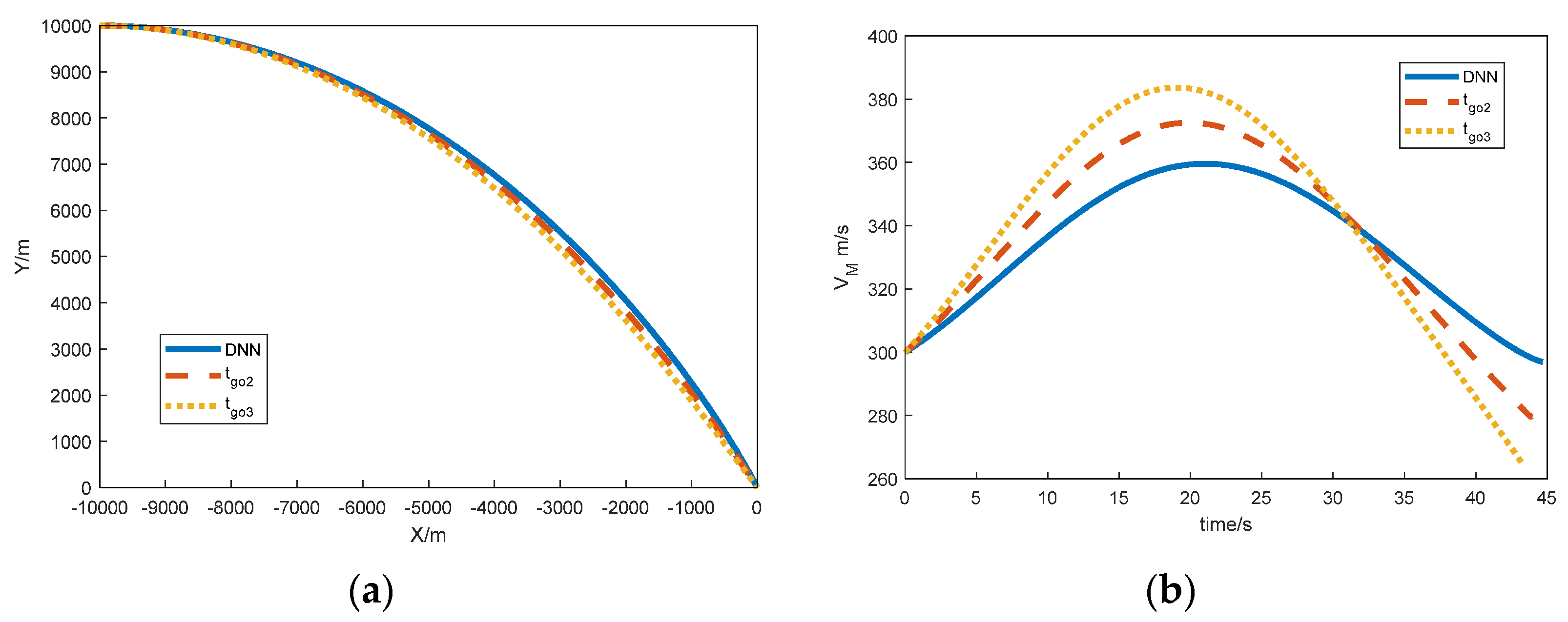
To verify the significant advantages of the bias term estimated by the DNN model compared to the traditional methods, different solution forms were tested for calculating the total flight time, as shown below:

$$t_2=\frac{R}{V_M}[1+\frac{\sin {\lambda }^2}{2(2N-1)}]$$

(39)

$$t_3=\frac{R}{V_M}(1+\frac{2{\lambda }^2+\lambda (q_f-q)+2{(q_f-q)}^2}{30})$$

(40)

The initial velocity was set to $300 \mathrm{m}/\mathrm{s}$, and the target coordinates were $(0,0)$. The remaining simulation parameters are shown in

Table 5. Initial flight vehicle conditions.

Initial Flight Vehicle Position/m	Navigation Gain	Maximum Acceleration (m/s2)	Initial Flight Path Angle/°	Desired Impact Angle/°
(−10,000, 10,000)	3	20	0	−70

.

The simulation results are shown in Figure 10.

The miss distance and actual impact angle for the three scenarios are shown in

Table 6. Miss distance and impact angle.

Scenario	Miss Distance/m	Final Impact Angle/°
DNN	0.04	−69.87
$t_{go2}$	0.11	−65.62
$t_{go3}$	0.02	−62.06

.

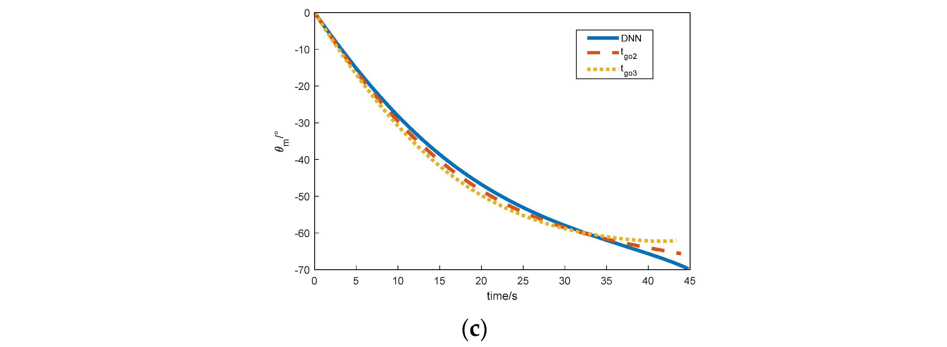
Figure 10 and Table 6 show that although all three cases hit the target, and the final impact angle obtained by the DNN model designed in this study is closer to the desired impact angle than the traditional method, the difference is only 0.13°. This indicates that the accuracy of the estimated bias term of DNN model was higher. Next, we will compare and simulate with the varying-speed method to further verify the advantages of the proposed method in this paper. A method for varying-speed estimation is proposed in [31].

$$t_4=\frac{R}{\overline{V}(x)}\left[1+\frac{{\lambda }^2}{2(2N-1)}\right]$$

(41)

where

$$\begin{array}{cc}\overline{V}(x)& =\frac{1}{x_{\mathrm{f}}-x_0}{\displaystyle {\int }_{x_0}^{x_{\mathrm{f}}}V(x)dx}\hfill \\ & =\frac{1}{4}{h}_1{\left(x_{\mathrm{f}}-x_0\right)}^3+\frac{1}{3}{h}_2{\left(x_{\mathrm{f}}-x_0\right)}^2+\frac{1}{2}{h}_3\left(x_{\mathrm{f}}-x_0\right)+h_4\hfill \end{array}$$

(42)

The meanings represented by each parameter are explained in [31] and will not be elaborated here. The specific simulation parameters are shown in

Table 7. Initial flight vehicle conditions.

Initial Flight Vehicle Position/m	Navigation Gain	Maximum Acceleration (m/s2)	Initial Flight Path Angle/°	Desired Impact Angle/°
(−8500, 8500)	3	20	0	−70

.

The simulation results are shown in Figure 11.

The simulation results for the two scenarios are shown in

Table 8. Simulation results.

Scenario	Miss Distance/m	Final Impact Angle/°	Final Velocity (m/s)	Operation Step Size/s
DNN	0.08	−69.85	320	0.002
$t_{go4}$	0.20	−71.49	325	0.9

.

From Figure 11 and Table 8, it can be seen that both methods can hit the target. Although the method proposed in this paper is closer to the desired impact angle compared to the method in [31], the difference is not significant. The advantage of this paper mainly lies in the fact that, as shown in Equation (4), the integral operation equation was used to calculate $\overline{V}(x)$, which requires a large amount of computation. The simulation results were also conducted on the simulation platform in Section 5.1. The calculation time for each step using the method described in this article is 2 ms, while in [31], this is 900 ms. It is obvious that this cannot be achieved on flight-vehicle-borne computers. Therefore, the method proposed in this article can reduce the computational load of flight-vehicle-borne computers and lower computational costs.

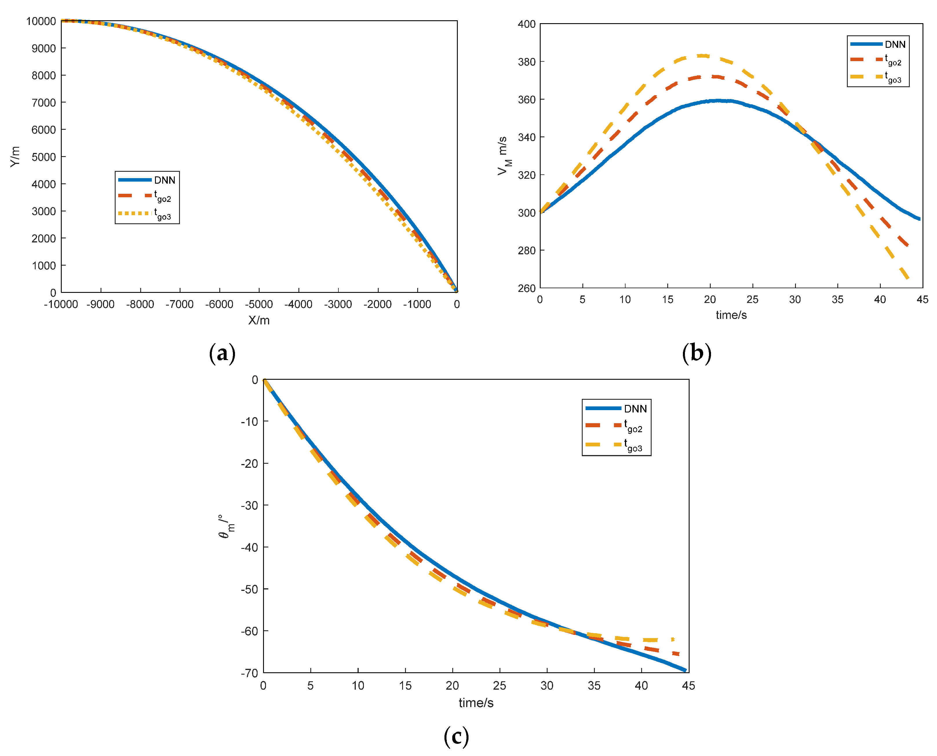
5.5. Comparison under Noise Interference

When considering the angle measurement from the seeker, the seeker’s uncertainty needs to be considered. Taking a typical radar seeker as an example, the uncertainty of the seeker mainly includes flicker noise and receiver noise. In general, this can be considered as Gaussian white noise. Based on the simulation parameters in Section 5.4, white noise with a mean of 0 and a variance of 0.6°/s was introduced in the seeker measurement information. The simulation results with the same parameters as in Section 5.2 are shown in Figure 12.

The miss distance and actual impact angle for the three scenarios are shown in

Table 9. Miss distance and impact angle.

Scenario	Miss Distance/m	Impact Angle/°
DNN	0.07	−69.58
$t_{go2}$	0.05	−66.12
$t_{go3}$	0.01	−61.54

.

Figure 12 and Table 9 show that although all three cases hit the target, and the final impact angles obtained by the DNN model designed in this study were closer to the desired impact angles than those by the traditional methods, the difference is only $0.42°$. This result demonstrates that the DNN model in this paper provides higher precision in estimating the bias term. Compared to the case without noise, although the actual impact angles are greater, the difference is only $0.29°$, demonstrating the robustness of the DNN model designed in this study.

6. Conclusions

This paper proposes an L-BPN method that uses the minimum amount of data possible for IACG. The key to the method is to maintain high prediction accuracy and validity while applying the minimum amount of data. In this paper, the mapping relationship between the bias term and the terminal fall angle is theoretically derived and proved. Through sensitivity analysis, the minimum amount of data can be applied to reduce training time while ensuring accuracy. Furthermore, the application of DNN for offline training and its capability for online deployment are explored. The simulation results show that the method can obtain more accurate impact angles with less errors than the traditional method.

References

1. Ratnoo, A.; Ghose, D. Impact angle constrained interception of stationary targets. J. Guid. Control. Dyn. 2008, 31, 1817–1822. [Google Scholar] [CrossRef]
2. Li, Q.; Yan, T.; Gao, M.; Fan, Y.; Yan, J. Optimal Cooperative Guidance Strategies for Aircraft Defense with Impact Angle Constraints. Aerospace 2022, 9, 710. [Google Scholar] [CrossRef]
3. Wang, Y.; Wang, W.; Lei, H.; Liu, J.; Chen, B.; Yin, Z. Observer-based robust impact angle control three-dimensional guidance laws with autopilot lag. Aerosp. Sci. Technol. 2023, 141, 108505. [Google Scholar] [CrossRef]
4. Li, H.; Wang, J.; He, S.; Lee, C.H. Nonlinear optimal impact-angle-constrained guidance with large initial heading error. J. Guid. Control. Dyn. 2021, 44, 1663–1676. [Google Scholar] [CrossRef]
5. Li, B.; Tang, P.; Xu, H.; Zheng, D. Terminal Impact Angle Control Guidance Law Considering Target Observability. Aerospace 2022, 9, 193. [Google Scholar] [CrossRef]
6. Lee, C.H.; Kim, T.H.; Tahk, M.J.; Whang, I.H. Polynomial guidance laws considering terminal impact angle and acceleration constraints. IEEE Trans. Aerosp. Electron. Syst. 2013, 49, 74–92. [Google Scholar] [CrossRef]
7. Zhang, Y.; Wang, X.; Ma, G. Impact time control guidance law with large impact angle constraint. Proc. Inst. Mech. Eng. Part G J. Aerosp. Eng. 2015, 229, 2119–2131. [Google Scholar] [CrossRef]
8. Chen, X.; Wang, J. Optimal control based guidance law to control both impact time and impact angle. Aerosp. Sci. Technol. 2019, 84, 454–463. [Google Scholar] [CrossRef]
9. Dong, W.; Wang, C.; Liu, J.; Wang, J.; Xin, M. Three-dimensional vector guidance law with impact time and angle constraints. J. Frankl. Inst. 2023, 360, 693–718. [Google Scholar] [CrossRef]
10. Chen, Z.; Chen, W.; Liu, X.; Cheng, J. Three-dimensional fixed-time robust cooperative guidance law for simultaneous with impact angle constraint. Aerosp. Sci. Technol. 2021, 110, 106523. [Google Scholar] [CrossRef]
11. Kumar, S.R.; Rao, S.; Ghose, D. Nonsingular terminal sliding mode guidance with impact angle constraints. J. Guid. Control. Dyn. 2014, 37, 1114–1130. [Google Scholar] [CrossRef]
12. Chen, S.; Wang, W.; Fan, J.; Ji, Y. Impact angle constraint guidance law using fully-actuated system approach. Aerosp. Sci. Technol. 2023, 136, 108220. [Google Scholar] [CrossRef]
13. Wang, X.; Lan, G.; Yang, Y.; Lu, H.; Huang, X. Terminal angle constrained time-varying sliding mode guidance law with autopilot dynamics and input saturation. Asian J. Control 2023, 25, 1130–1144. [Google Scholar] [CrossRef]
14. Kim, T.H.; Park, B.G.; Tahk, M.J. Bias-shaping method for biased proportional navigation with terminal-angle constraint. J. Guid. Control. Dyn. 2013, 36, 1810–1816. [Google Scholar] [CrossRef]
15. Ratnoo, A. Analysis of two-stage proportional navigation with heading constraints. J. Guid. Control. Dyn. 2016, 39, 156–164. [Google Scholar] [CrossRef]
16. Wang, Y.; Wang, H.; Lin, D.; Wang, W. Nonlinear modified bias proportional navigation guidance law against maneuvering targets. J. Frankl. Inst. 2022, 359, 2949–2975. [Google Scholar] [CrossRef]
17. Cho, N.; Kim, J.; Lee, S.; Kim, Y. Generalized analysis of biased proportional navigation guidance with fractional power error feedback. J. Guid. Control. Dyn. 2022, 45, 1598–1613. [Google Scholar] [CrossRef]
18. Su, W.; Yao, D.; Li, K.; Chen, L. A novel biased proportional navigation guidance law for close approach phase. Chin. J. Aeronaut. 2016, 29, 228–237. [Google Scholar] [CrossRef]
19. Cheng, L.; Jiang, F.; Wang, Z.; Li, J. Multiconstrained real-time entry guidance using deep neural networks. IEEE Trans. Aerosp. Electron. Syst. 2020, 57, 325–340. [Google Scholar] [CrossRef]
20. Song, E.J.; Lee, H.; Tahk, M. On-line suboptimal midcourse guidance using neural networks. In Proceedings of the 35th SICE Annual Conference. International Session Papers, Tottori, Japan, 24–26 July 1996; pp. 1313–1318. [Google Scholar]
21. Filici, C.; Peña, R.S.S. Online guidance updates using neural networks. Acta Astronaut. 2010, 66, 477–485. [Google Scholar] [CrossRef]
22. Liang, C.; Wang, W.; Liu, Z.; Lai, C.; Zhou, B. Learning to guide: Guidance law based on deep meta-learning and model predictive path integral control. IEEE Access 2019, 7, 47353–47365. [Google Scholar] [CrossRef]
23. Christopher Frey, H.; Patil, S.R. Identification and review of sensitivity analysis methods. Risk Anal. 2002, 22, 553–578. [Google Scholar] [CrossRef]
24. Zhang, T.; Su, J.; Liu, C.; Chen, W.H. State and parameter estimation of the AquaCrop model for winter wheat using sensitivity informed particle filter. Comput. Electron. Agric. 2021, 180, 105909. [Google Scholar] [CrossRef]
25. Borgonovo, E.; Plischke, E. Sensitivity analysis: A review of recent advances. Eur. J. Oper. Res. 2016, 248, 869–887. [Google Scholar] [CrossRef]
26. Tipàn, S.; Theodoulis, S.; Thai, S.; Proff, M. Nonlinear dynamic inversion flight control design. J. Guid. Control. Dyn. 2020, 43, 975–980. [Google Scholar] [CrossRef]
27. Ryoo, C.K.; Cho, H.; Tahk, M.J. Time-to-go weighted optimal guidance with impact angle constraints. IEEE Trans. Control. Syst. Technol. 2006, 14, 483–492. [Google Scholar] [CrossRef]
28. Dhananjay, N.; Ghose, D. Accurate time-to-go estimation for proportional navigation guidance. J. Guid. Control. Dyn. 2014, 37, 1378–1383. [Google Scholar] [CrossRef]
29. Liu, C.; Fan, W.; Li, J.; Zhu, Z. Desired Impact Time Range Based on BP Neural Network. In Proceedings of the China Conference on Command and Control, Nanjing, China, 25–27 November 2023; Springer Nature: Singapore, 2023; pp. 171–181. [Google Scholar]
30. Liu, Z.; Wang, J.; He, S.; Shin, H.S.; Tsourdos, A. Learning prediction-correction guidance for impact time control. Aerosp. Sci. Technol. 2021, 119, 107187. [Google Scholar] [CrossRef]
31. Guoxin, S.; Qiuqiu, W.; Zhiqiang, X.; Qunli, X. Impact time control using biased proportional navigation with varying velocity. Chin. J. Aeronaut. 2020, 33, 956–964. [Google Scholar]
Figure 1. Relative motion model of flight vehicle and target.
Aerospace 11 00376 g001
Figure 2. The impact of parameter on b . (a) The impact of x 0 on b ; (b) the impact of N on b ; (c) the impact of θ f on b ; (d) the impact of y 0 on b ; (e) the impact of V m 0 on b ; (f) the impact of θ 0 on b .
Aerospace 11 00376 g002
Figure 3. DNN structure.
Aerospace 11 00376 g003
Figure 4. Overall architecture.
Aerospace 11 00376 g004
Figure 5. Comparison of two cases. (a) Comparison of training set; (b) comparison of test set.
Aerospace 11 00376 g005
Figure 6. Accuracy on the test set.
Aerospace 11 00376 g006
Figure 7. Accuracy on the test set. (a) Flight trajectory; (b) velocity curve; (c) flight path angle.
Aerospace 11 00376 g007aAerospace 11 00376 g007b
Figure 8. Flight trajectory.
Aerospace 11 00376 g008
Figure 9. Monte Carlo simulation results.
Aerospace 11 00376 g009
Figure 10. Simulation results comparing the three methods. (a) Flight trajectory; (b) velocity curve; (c) flight path angle.
Aerospace 11 00376 g010aAerospace 11 00376 g010b
Figure 11. Simulation results comparing the two methods. (a) Flight trajectory; (b) velocity curve; (c) flight path angle.
Aerospace 11 00376 g011
Figure 12. Simulation results comparing the three methods. (a) Flight trajectory; (b) velocity curve; (c) flight path angle.
Aerospace 11 00376 g012