Article

Fault-Tolerant Control for Multi-UAV Exploration System via Reinforcement Learning Algorithm

1
School of Aeronautics and Astronautics, Zhejiang University, Hangzhou 310027, China
2
Department of Mathematics, The University of Manchester, Manchester M13 9PL, UK
*
Author to whom correspondence should be addressed.
Aerospace 2024, 11(5), 372; https://doi.org/10.3390/aerospace11050372
Submission received: 21 March 2024 / Revised: 24 April 2024 / Accepted: 6 May 2024 / Published: 8 May 2024
(This article belongs to the Section Aeronautics)

Abstract

:
In the UAV swarm, the degradation in the health status of some UAVs often brings negative effects to the system. To compensate for the negative effect, we present a fault-tolerant Multi-Agent Reinforcement Learning Algorithm that can control an unstable Multiple Unmanned Aerial Vehicle (Multi-UAV) system to perform exploration tasks. Different from traditional multi-agent methods that require the agents to remain healthy during task execution, our approach breaks this limitation and allows the agents to change status during the task. In our algorithm, the agent can accept both the adjacency state matrix about the neighboring agents and a kind of healthy status vector to integrate both and generate the communication topology. During this process, the agents with poor health status are given more attention for returning to normal status. In addition, we integrate a temporal convolution module into our algorithm and enable the agent to capture the temporal information during the task. We introduce a scenario regarding Multi-UAV ground exploration, where the health status of UAVs gradually weakens over time before dropping into a fault status; the UAVs require rescues from time to time. We conduct some experiments in this scenario and verify our algorithm. Our algorithm can increase the drone’s survival rate and make the swarm perform better.

1. Introduction

Unmanned Aerial Vehicles (UAVs) have become widely used in our daily lives and industry applications [1]. Multi-UAV exploration [2] is one of the most important applications in the UAV industry. It can be used to measure forest cover, wildlife migration, and natural disaster assessment. UAVs have broad prospects in the field of exploration.
In large-scale exploration, the UAV swarm plays an important role [3] in enhancing exploration efficiency and mission reliability. However, UAV swarm exploration needs to deal with a lot of challenges, such as Multi-UAV coordination and fault handling. Because of the large number of UAVs, there are some UAVs that may encounter errors (like poor battery, among others), and there are more challenges to cooperate between UAVs.
Some studies are approaching this problem with respect to the collaboration between multiple UAVs [4,5]. For instance, reference [6] investigated aerial combat scenarios involving multiple UAV collaboration; the authors used the Ray framework to train a MAPPO algorithm, which achieved excellent performance in aerial combat scenarios. The authors in [7] explored the possibility of swarm cooperation in an environment where the channel is noisy and communication is interrupted. The authors of [8] proposed a hierarchical group communication model, which uses prior domain knowledge to schedule and control heterogeneous agent swarms. The work of [9] investigated the impact of partial agent loss on the collective behavior of multi-agent systems. The work of [10] investigated a fault-tolerant approach that can deal with agents with malicious behavior in the swarm. The work of [11] presentd a fault-tolerant control approach, which can predict actuator failures in UAVs and provide a control strategy. The work of [12] investigated adaptive strategies for UAV formations when tracking targets in the event of UAV failure or loss. The work of [13] proposed a robust control of the UAV: the controller can control the tracking flight of a UAV in an uncertain and external disturbances environment. The work of [14] proposed a control approach for agent swarms in extremely noisy environments. The work of [15] proposed a multi-agent algorithm that can evaluate the credibility of an agent’s observation and tolerate the inaccurate information observed by the agent. The work of [16] investigated how to control a multi-agent systems when the links between agents are lost. The work of [17] investigated the reconstruction of communication topology for UAV swarms with a minimal cost in the case of UAV loss. The authors of [18] discussed the methods to maintain the stability of a UAV swarm in the case of actuator failures or communication disruption. The authors of [19] developed a fault-tolerant cooperation framework for UAVs, which can reassign the tasks to make the swarm of UAVs more robust to uncertainties. The work of [20] proposed a fault-tolerant cooperative control strategy that can decrease the effects of the changed formation and reassign the faulty UAV’s tasks to the healthy ones. The authors of [21] proposed a priority-based strategy for finding a substitute UAV in the swarm when a UAV is lost.
The existing publications focus on how to keep the balance of the system when some agents meet failure in the swarm. However, they designed fault-tolerant algorithms that only focus on the healthy agents and do not use the valuable information from faulty agents. We use the information not only from the healthy agents but also from the faulty agent to make decisions. During the process of aggregating information, most of the algorithms consider the type of neighboring agents, but we also consider the health status of the neighboring agents; this makes our work more targeted in fault-tolerant scenarios. In many designs, the faulty agents can only leave the swarm and abort the task, but in our design, we preserve the possibility of faulty agents reverting to the missions.
In this paper, we apply our algorithm in the scenario of large-scale UAV swarm exploration in the forest. A swarm of UAVs needs to cover a certain area and complete the exploration mission. In large-scale UAV swarms, some UAVs would be unhealthy and meet some malfunctions during the tasks; these kinds of UAVs would be unable to continue executing the task. The health status of UAVs becomes weak with the consumption of batteries in the tasks. When the energy drops below the threshold, the drone will enter a “tired” failure state (the Error State). They need to land and repair (such as recharge) before continuing the task. The faulty agents need the healthy agents’ help to return to the task. The fault-tolerant multi-agent scenario with abnormal states of agents is shown as Figure 1.
We study UAV swarm exploration with heterogeneous health status. We apply machine learning to the task of Multi-UAV exploration. We propose a kind of novel network model named Error-Resilience Graph Network (ERGN), which can tolerate the failure status in the UAV swarm and combine it with the health status of UAVs to inspire the collaborative capability of the UAV swarm.
The main contributions of this paper are as follows:
(1)
We simulate a Multi-UAV exploration scenario in a grid world. Faulty UAVs will occur in the scenario, which are used to verify the performance of our algorithm.
(2)
We propose a novel network model named Error-Resilience Graph Network (ERGN); it can receive the agent health status and conduct a scheduling policy to reduce the impact that faulty agents bring to the swarm target.
(3)
We integrate a temporal convolution module into the algorithm, which enables the agents to capture the temporal information and achieve better performance.

2. Methods

2.1. Dependence

2.1.1. Multi-Agent Reinforcement Learning (MARL)

Multi-Agent Reinforcement Learning (MARL) is an active research area [22]. It focuses on using reinforcement learning to make the agents learn to cooperate with neighbors for the global target [23]. MARL is widely used in different areas, such as traffic management, UAVs scheduling, etc. In different frameworks, agents adopt different decision-making methods [24]. Some agents use a centralized decision-making approach, while others employ a distributed decision-making method. Additionally, some agents utilize a hierarchical decision-making approach [25]. In terms of implementation, reinforcement learning can be classified into two main categories based on different learning patterns. The first one is Value-Based reinforcement learning, and the second one is Policy Gradient reinforcement learning. The first one is based on the value function to learn the strategy: when you input a state, the neural network will calculate the value for each possible selected action. Then, the policy chooses the highest value action to execute. During the training process, the agent will gradually learn the value distribution of selecting different actions in the states. After training, the agent will learn an accurate value, which can help the agent to obtain the highest reward. The second method is Policy Gradient reinforcement learning [26]; it receives the state of the agent and outputs action for the agent. The policy network will use the state to generate a distribution of probability for different actions; the better action has a higher probability of being chosen. In this way, the policy can choose effective actions. During the learning process, the policy uses the reward to optimize the probabilities of selecting actions. Positive behaviors are more likely to be chosen in the next iteration, while negative behaviors are less likely to be selected. After training, the probability distribution generated by the policy will be sufficiently efficient.
Applying reinforcement learning to multi-agent systems [27] is an extension of the learning approach for single agents. Of course, a single policy can also be used to control multiple agents with joint actions [28]. However, this approach is less commonly applied because of its weakness, it is difficult for the policy to make decisions independently for different agents, and the high dimensional output of the policy makes the training process very difficult. Multi-agent reinforcement learning is primarily based on single-agent reinforcement learning through establishing parameter sharing or parameter-independent mechanisms to reduce training difficulty. The parameter-independent mechanism [29,30] allows each agent to have an independent policy. During the training process, each agent updates its own policy until it learns how to cooperate with neighbors for the global target. The parameter sharing mechanism [31] uses the same policy for every agent: each agent collects the experience data and pushes them into the buffer. When the buffer has enough experience data, the policy network optimizes the network parameters periodically. After the training process, the policy will be distributed to different agents independently. The centralized training with a distributed execution approach has several advantages in the system, where each agent has identical functions and can accelerate convergence. On the other hand, it exhibits higher flexibility during distributed deployment, which can be suitable for systems with different numbers of agents. Our work is based on the parameter sharing mechanism and uses the DQN as the foundational algorithm to construct multi-agent reinforcement learning. In order to improve the performance, some multi-agent reinforcement learning algorithms combine with the communication mechanisms, thereby obtaining the neighbor’s information through communication to achieve collaboration purposes. In this aspect, our predecessors have accomplished an amount of work, which includes the graph attention mechanism [32], soft–hard attention mechanism [33], and GraphSAGE [34] as the aggregator. In the attention mechanism, the agent collects the neighbor’s information and judges the importance of the information. The important information will be given more weight, and the unimportant information will be given less weight. GraphSAGE deals with the problem in a similar way, but it takes individual agents as the smallest units. It uses the pooling layer to distribute different weights to different agents. The soft–hard attention is a compromise between these two strategies; it can exhibit better performance in some situations.

2.1.2. Deep Q Network (DQN)

DQN is a decision policy based on value functions in reinforcement learning [35]. It can deal with continuous and complex state spaces, but DQN does not output the action directly. DQN outputs the value of different actions that can be taken in the state, and it selects the action to be executed based on the value of each action. DQN uses the Q network to output the value of each action. The learning process is to optimize the Q network and use the Q network to make decisions; the decision policy can be described as π ( s ) = argmax a Q π ( s , a ) . There are two kinds of methods to optimize the Q network: the first one is the Monte Carlo (MC) optimization method, and the other is the Temporal Difference (TD) optimization method. In the training process, the TD method is more popular because of its stable convergence. On the other hand, the MC method needs to finish the episode and use the full trajectory of the agent to optimize the Q network, which has a greater randomness and leads to unstable training. The optimization process of the TD method can be shown like this: Q π s t , a t r t + Q π s t + 1 , π s t + 1 . In ideal cases, the left side of the equation equals the right side. However, in practice, there will be biases in the network’s predictions; we utilize these biases to calculate the loss and optimize the network. We use the results calculated on the right side as the optimization objective, Q t a r g e t = r t + Q π s t + 1 , π s t + 1 , and the left side is calculated as the prediction: Q e x p e c t = Q π s t , a t . The calculation of loss is L o s s = ( Q t a r g e t Q e x p e c t ) 2 .

2.1.3. Graph Attention Networks (GATs)

Graph Attention Networks are primarily used for processing information in the spatial domain; they can be used to deal with the information data with graph topology relationships [36]. GATs assign different weights to different nodes in the graph topology and aggregate valuable information to form a feature vector. After that, the policy network uses the feature vector for decision making. GATs use the attention mechanism to assign weights to neighbor nodes; the important neighbor nodes are given higher attention weights. GATs obtain the observation for each agent as x i and use an embedding layer to convert them into a i . Then, the neural networks are based on a i to generate q i , k i , and v i . The q and k are paired keys that work together to generate attention weights, which are defined as α i , j = q i T · k j d q , k . In order to keep the attention weights α i , j in the range of 0–1, we also apply a softmax operation to them, which is defined as α ^ i , i = Softmax α i , i . Then, the GAT multiplies α i , j and v j to generate the feature vector b i , b i = j = 1 T α ^ i , j · v j , for decision making.

2.1.4. Long Short-Term Memory (LSTM)

Long Short-Term Memory has widespread applications in the field of deep learning, especially in areas such as natural language processing and time series prediction. LSTM is a recurrent neural network used to integrate historical information in a temporal sequence [37]. In comparison to traditional Recurrent Neural Networks, LSTM includes an additional temporal chain to capture long-term information. The long-term chain and short-term chain interact with each other, thus allowing the short-term chain to modify the content on the long-term chain based on the input information. The deletion operation is implemented through a formula, f 1 = sigmoid ( w 1 [ h t 1 , x t ] + b 1 ) , where h t 1 is the output of the short-term memory chain from the previous time step, and x t is the input at the current time step. The addition operation is implemented through this formula: f 2 = sigmoid ( w 2 [ h t 1 , x t ] + b 2 ) tanh ( w ^ 2 [ h t 1 , x t ] + b ^ 2 ) . Finally, the long-term feature vector is generated by c t = c t 1 f 1 + f 2 , and the short-term feature vector is generated by h t = tanh ( w 3 c t + b 3 ) sigmoid ( w ^ 3 [ h t 1 , x t ] + b ^ 3 ) . The c t and h t will transfer to the next inference cycle. With the help of long-term memory c t and short-term memory h t , the policy network can make decisions considering both the current state and historical state.

2.2. System Model

2.2.1. Ground Exploration Scenario

In this section, we propose the UAV ground exploration task and detail the design of the ground exploration scenario. Ground exploration is one of the important applications of UAVs. UAVs equipped with sensing devices are deployed and conducted to scan the ground areas within a limited time. This method assists the command center to obtain the information about the terrain conditions or equipment deployment in these areas. When carrying out these missions, the work teams dispatch UAV swarms to conduct joint operations to ensure the efficiency of mission execution. We designed a scenario for the exploration mission, which consists of an L*L grid area. The UAVs conduct exploration missions in the area; when the UAV reaches a grid, it completes the exploration of the grid, and there is no additional benefit for repeated exploration. At the same time, the UAVs can establish communications with each other, and they can exchange information if they are within communication range of each other. Each one has a health status that decreases as the battery energy is consumed, and when the health status drops below a threshold the drone will fall into a faulty status, and then the UAV needs to land and repair for the next flight. Affected by the exploration terrain, the faulty UAV requires assistance from other UAVs to resume flight. When the neighboring UAVs approach the faulty UAV, they repair the faulty UAV and share the environmental information. The faulty UAV can take off and recover to the exploration mode. In many cases, the appearance of faulty UAVs would lead to the ineffective execution of the decision policy. How to deal with the faulty UAVs becomes the key to improve the task completion. The exploration process is shown in Figure 1.

2.2.2. Observation Space and Action Space

Each UAV has its own observation space and action space; the observation content coming from the environment will be used as the input of the policy network to make action decisions. The observation space consists of several components, including the UAV’s health status, binary encoding of its x-axis position and y-axis position, the encoding of observation information, and the encoding of information about the distribution of the neighboring UAVs within the communication range. The health status refers to the battery level of the UAV. The action space is discrete: each UAV has five action options, which include forward, backward, leftward, rightward, and hover movements. At each time step, the UAV can obtain a set of observational space information and a set of action space information. What is more, we also designed a matrix to describe the communication relationships between the UAVs and a vector to describe the health status of the UAVs. The communication matrix is an n × n matrix (n means the number of the UAVs), and each element of the matrix means the connectivity. If the element is 1, these two UAVs are able to share information with each other; if the element is 0, there is no communication channel between these two UAVs. The health vector is an n-dimensional vector, which is used to describe the health status of the UAVs—normal or fault. When the health status of the UAV is dropped below the threshold, the UAV will enter into a faulty status, and the flag in the vector will be set to 0; otherwise, the flag in the vector is 1. When the flag is 0, the corresponding UAV will lose the ability to move, and the action space will be invalid. The communication matrix and the health status vector are also updated at each time step.

2.2.3. Evaluation Metrics

The quality of the UAVs’ performance of exploration is decided by the efficiency of the UAVs. In the limited time steps, the more areas that the UAV explored, the better the performance. The exploration performance of the UAVs is determined by both the individual reward and the global reward. Individual performance means the number of new areas detected by a single UAV at a time step. The UAVs are encouraged to explore new areas instead of staying in the same place. When the agent explores a new area, the reward will increase by 10 points.
individual _ reward = ( new _ areas ) 10
At the same time, the UAV also needs to learn to consider the global benefit by exploring more areas by cooperating with each other. In this aspect, the global performance is considered in the reward function.
global _ reward = ( total _ areas + expored _ areas ) / 100
The more explored areas, the higher the global reward. Flying out of the mission areas is not supported, so we designed a penalty factor.
penalty _ factor = ( hit _ barriers ) 10
If the UAV tends to get out of the mission areas, the agent will be punished. Overall, the reward of the agent consists of the individual reward, global reward, and the penalty factors.
reward = individual _ reward + global _ reward + penalty _ factor

2.3. Error-Resilient Graph Network

Many existing algorithms only consider the health agents. In other words, the agents never meet accidents throughout the whole task execution. However, in some cases, the agent will go into the faulty status with the decline of its health status. We propose the Error-Resilient Graph Network (ERGN). The ERGN can deal with the different status levels of the agents, and the network model can not only receive the adjacency matrix about the agent communication but also receive the vector about the agent health status.
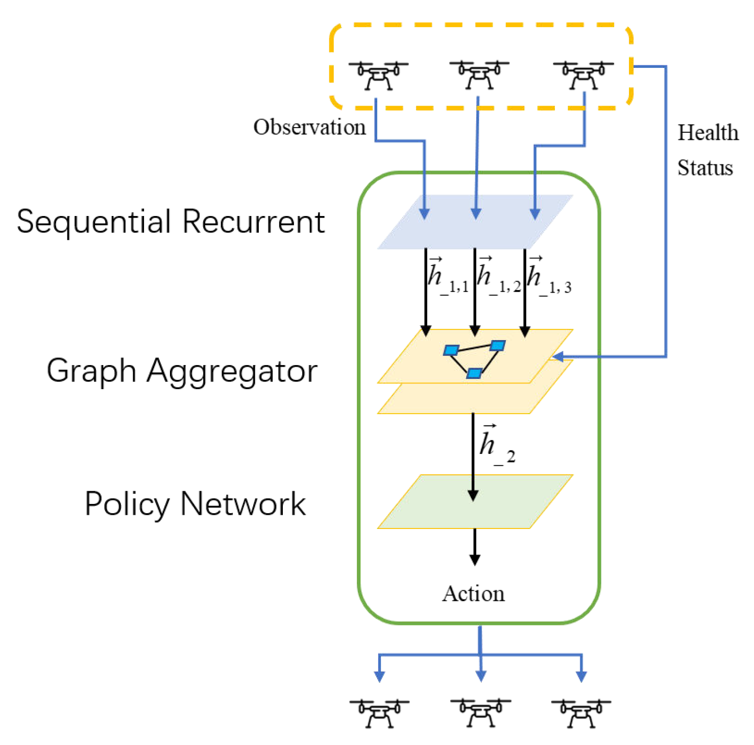
The policy will adopt different behavioral strategies as the agent status changes. The ERGN employs a novel approach to process the neighbor relationship matrix. The relationship matrix between agents will be adjusted along with the health status of the agent. When an agent falls into a faulty status, the neighbor agents will establish a rescue team and pay more attention to the faulty agent. They work together to repair the faulty agent. In the following sections, we will introduce our network from two perspectives: the processing of spatial information and the processing of temporal information. The framework of the ERGN is depicted in Figure 2. The h _ t , i in the figure means the hidden state of agent i in step t.

2.3.1. Spatial Information Aggregation

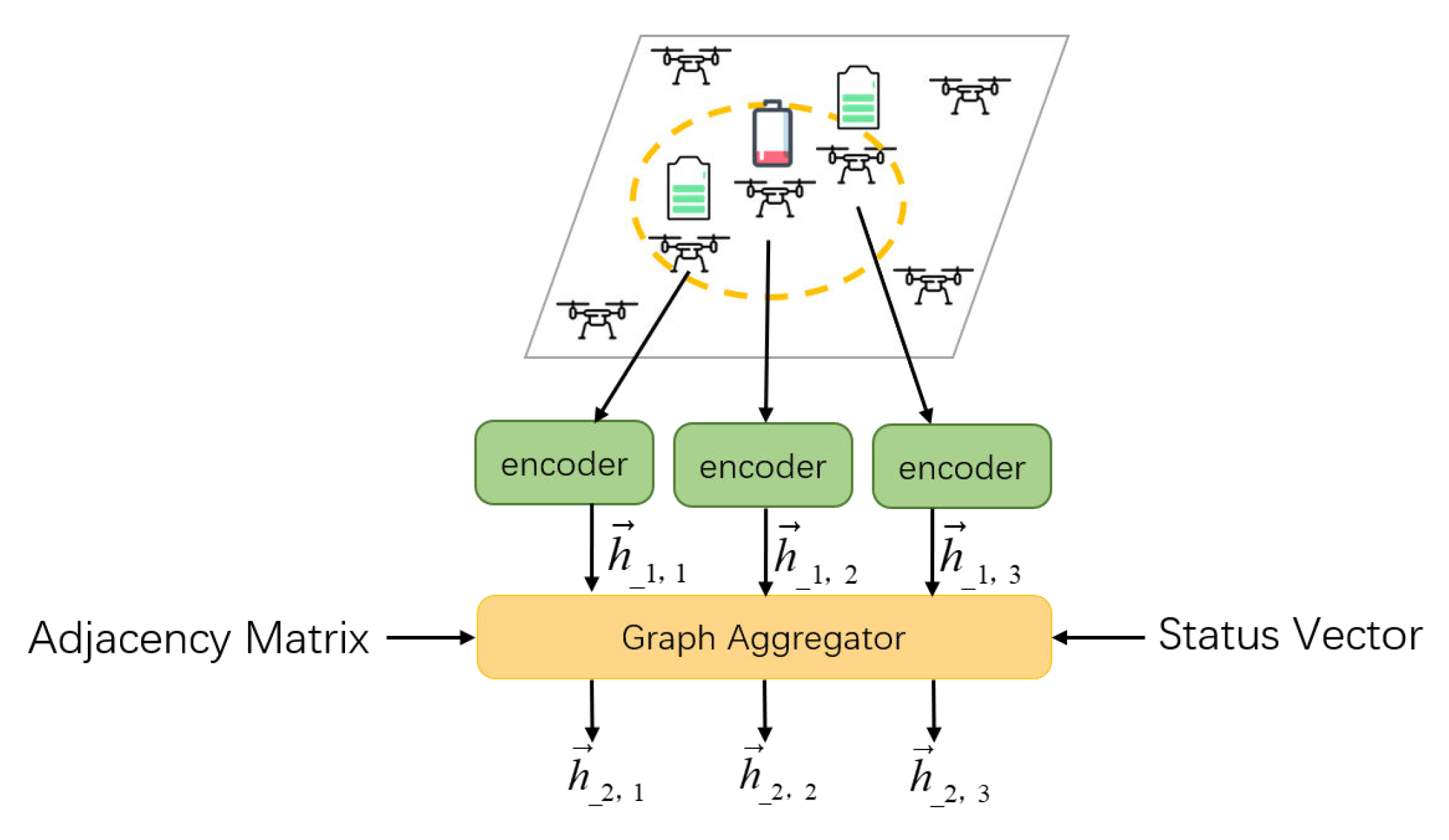
In our ERGN model, the spatial information is aggregated by the GAT module. In this scenario, the UAV has the ability to communicate with its companions. The agent can not only sense the local observations but also utilize the neighbor observations through the communication channels. The aggregated results will be used for decision making. The aggregator module receives information from three sources, including the observation encoding, the communication matrix, and the vector of the agents health status, as shown in Figure 3.
The encoder module encodes the information from the observations of agents, compresses observations, and extracts feature vectors to a uniform dimension as h . The process can be shown as follows, where x is the observation of agents, and W is an MLP with 32 dimensions of input and 128 dimensions of output.
h i = R e L U W x i
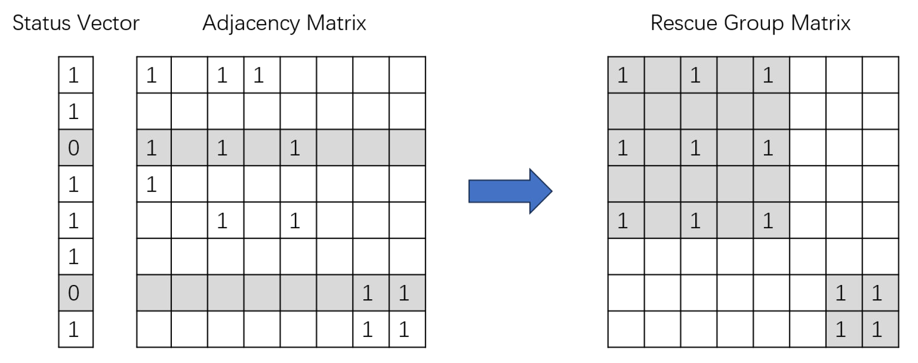
After that, the Graph Aggregator receives the information from three sources to aggregate a new feature vector. When all of the elements in the status vector are 1, it means that all agents are staying at the normal status. However, when some elements in the state vector are 0, it means some agents fall into a faulty status; the aggregator will use the adjacency matrix and status vector to generate a new mask matrix, and the new mask matrix can help the normal agents within the communication range of the faulty agent to establish a rescue team to restore the status of the faulty agent.
A = { a 1 , a 2 , , a n } a i f a u l t _ a g e n t
G = { g r o u p { a i } } a i A
g r o u p { a i } = a j j = { j N a i , j = 1 }
p a i r s { a i } = ( a x , a y ) a x g r o u p { a i } , a y g r o u p { a i }
R e s c u e _ G r o u p _ M a t r i x = M , M ( x , y ) = 1 ( x , y ) p a i r s { a i }
This process is generated by the adjacency matrix and the status vector, which are shown in Figure 4. For example, agent 3 is in the faulty state and it has two neighbors (agent 1 and agent 5); thus, agents 1, 3, and 5 build up a rescue group (the shadow block in the upper left corner of the rescue matrix), and agents staying in the same group can communicate with each other with the help of agent 3. The rescue group matrix describes the communication between the agents in rescue groups, which contains the multi-hop communication with the help of agents waiting for rescue. In this way, the normal agent will abandon the information of neighboring agents and enhance the connections with other agents within the rescue team.
The aggregate process between the adjacency matrix and status vector can be described as follows: we can fetch the index of the faulty agents using a status vector and use the adjacency matrix to find out the index of the corresponding neighbor agents for the faulty agents to adjust the adjacency of the neighbor agents in the rescue group. The agents staying in the same group can share their information with each other. If one agent appears in two groups at the same time, these two groups will merge into one group, and agents within the group establish adjacency with each other. In this way, we rebuild the adjacency matrix through the adjacency relationship. This matrix will be used as input to the GAT module; the GAT aggregator then outputs the feature vectors for each agent. They are used to determine which action will be taken. The aggregate process can be shown as follows, where W is an MLP with 128 dimensions of input and 128 dimensions of output.
q i = W q h i ; k i = W k h i ; v i = W v h i
α i , j = q i T · k j d q , k ; α = α m a s k
α ^ i , j = Softmax α i , j ; b i = j = 1 T α ^ i , j · v j
h i = R e L U W b i

2.3.2. Temporal Information Aggregation

History information is also important for agents. While an intelligent agent is moving forward, some unknown areas along the way are discovered. However, it may not be possible to reach them at once due to the path planning. It is necessary to return and supplement after exploring other areas. Thus, we integrate the LSTM into our algorithm to further improve the performance. We use the LSTM module to convolve the observation for each step, which can help the policy to make decisions not only depending on the current states but also using the history information. The LSTM module receives current states h along with the hidden state from the last time step { H t 1 , C t 1 } and outputs the hidden state of the current step { H t , C t }. The current hidden state will be used for decision making at this time step and prepared for the next convolution. This process can be shown as follows:
f 1 = Sigmoid W 1 H t 1 , h t + b 1
f 2 = Sigmoid W 2 H t 1 , h t + b 2 tanh W ^ 2 H t 1 , h t + b ^ 2
C t = C t 1 f 1 + f 2
f 3 = tanh W 3 C t + b 3 Sigmoid W ^ 3 H t 1 , h t + b ^ 3
H t = f 3 ; h t = f 3
The decision-making process of the strategy network is shown in Figure 5. Graph Aggregator concats the long memory feature C and short memory feature H to produce a new feature vector. And the MLP layer uses the new feature vector to generate the value distribution of actions.

2.4. Training Process

During the training process of the neural network, we combine it with the simulated annealing algorithm. As the training process progresses, we continuously reduce the noise to reach a balance between exploration and exploitation. Our ERGN outputs deterministic action values, and deterministic action values can lead the agent to a lack of ability to explore, thus causing the training process to fall into a local optimum. Hence, we integrate some noise into the algorithm, and the noise will reduce gradually. At the first time, the probability of noise is 90%; only one in ten times will follow the action given by the policy network. More actions are generated randomly in order to encourage the agent exploration and collect the abandoned experience. Introducing too much noise can make the training process of the network difficult to converge. Therefore, we adopt the simulated annealing algorithm, and the added noise continuously decays with the training process until it reaches a lower level. When the noise reaches a lower level, the agent follows the instructions of the policy network, and the agent can complete the tasks effectively.
ϵ = ϵ δ for each episode
a c t i o n i = random action a i if x U ( 0 , 1 ) ; x < ϵ max a E R G N o b s , a d j , s t a t u s , h i d d e n _ s t a t e if x U ( 0 , 1 ) ; x ϵ
e x p e c t _ Q = E R G N ( o b s , a d j , s t a t u s , h i d d e n _ s t a t e ) t a r g e t _ Q = E R G N ( o b s , a d j , s t a t u s , h i d d e n _ s t a t e )
L o s s = ( e x p e c t _ Q a c t i o n ( r e w a r d + γ m a x t a r g e t _ Q ) ) 2
where ϵ is the probability of not following the policy network; this probability continuously decreases as the training process progresses. The ERGN obtains the observations, status of agents, neighbor matrix and hidden_state combined with history information to make decisions for each agent. o b s , a d j , s t a t u s , h i d d e n _ s t a t e means the next step information. Finally, we use the Q value of the action selected in the current time step and the Q value of the best action in the next time step to calculate the L o s s and optimize the neural network.
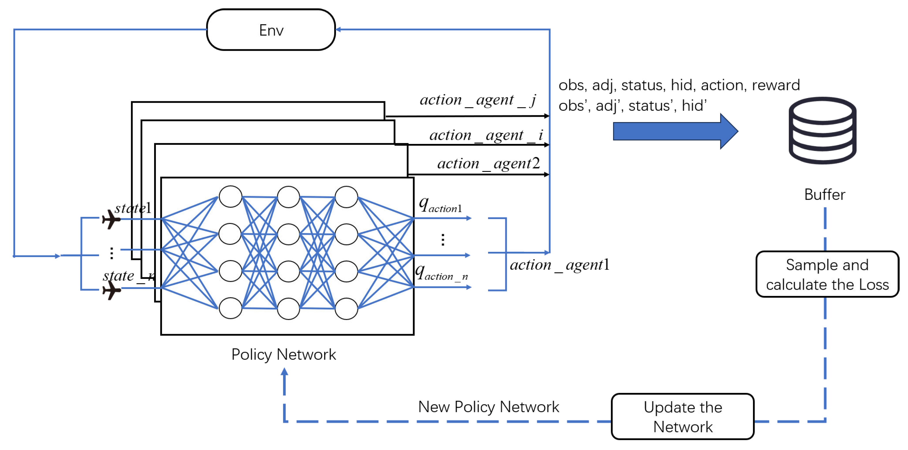
The training process is visualized in Figure 6. Firstly, we initialize the replay buffer, which is used to collect the experience data generated during the interaction between the agents and the environment. After that, we initialize the policy network; the policy network is used to generate actions for the agent. It takes the observations and status information of the agents as input and outputs the value weights for each action. Then, based on probabilities, it selects one action to execute. Finally, each agent receives an action for execution. These actions are transmitted to the environment and interact with the environment, and agents receive the state information of the next step. This iterative process continuously generates experience data. The experience data are pushed into the replay buffer in order to optimize the policy network. When the buffer contains enough data, the optimizer periodically samples some data to calculate the loss for optimizing the policy network. After that, the new policy replaces the original one to make decisions for the swarm. This process iterates until the policy network achieves good performance. Algorithm 1 describes the process of the ERGN:
Algorithm 1 Error-Resilient Graph Network
1:
Initialize replay buffer
2:
Initialize weights for ERGN, including graph aggregator, recurrent network, and policy networks
3:
Initialize weights for target ERGN , ERGN = ERGN
4:
for episode e p i = 1 to T do
5:
    Reset the environment and initialize the hidden state ( H i , C i ) for each agent i
6:
    for time steps t = 1 to episode length do
7:
        for agent i = 1 to N do
8:
            ( H i t , C i t ) L S T M ( o b s i t , ( H i t 1 , C i t 1 ) )
9:
            m a s k A G G R E G A T E ( a d j , s t a t u s )
10:
            h i G A T ( c o n c a t ( H i t , C i t ) , m a s k )
11:
           With probability ϵ select a random action a t
12:
           Otherwise select a i = argmax a Q π ( h i , a )
13:
           Execute agent’s action a i to the environment
14:
           Obtain r e w a r d , o b s , a d j , s t a t u s , h i d d e n _ s t a t e
15:
        end for
16:
        Collect the experience
17:
         e x p = [ a c t i o n , r e w a r d , o b s , o b s , a d j , a d j , s t a t u s , s t a t u s , h i d d e n _ s t a t e , h i d d e n _ s t a t e ]
18:
        Push the experience into the replay buffer
19:
         o b s = o b s , a d j = a d j , s t a t u s = s t a t u s , h i d d e n _ s t a t e = h i d d e n _ s t a t e
20:
    end for
21:
     ϵ = ϵ δ
22:
    for update epoch e p o c h = 1 to update times do
23:
        Sample a batch of experiences from the replay buffer
24:
         e x p e c t _ Q = E R G N ( o b s , a d j , s t a t u s , h i d d e n _ s t a t e )
25:
         t a r g e t _ Q = E R G N ( o b s , a d j , s t a t u s , h i d d e n _ s t a t e )
26:
         L o s s = ( e x p e c t _ Q a c t i o n ( r e w a r d + γ m a x t a r g e t _ Q ) ) 2
27:
        Update weights for ERGN network
28:
    end for
29:
    From time to time copy weights into the target network
30:
end for

2.5. Training Settings

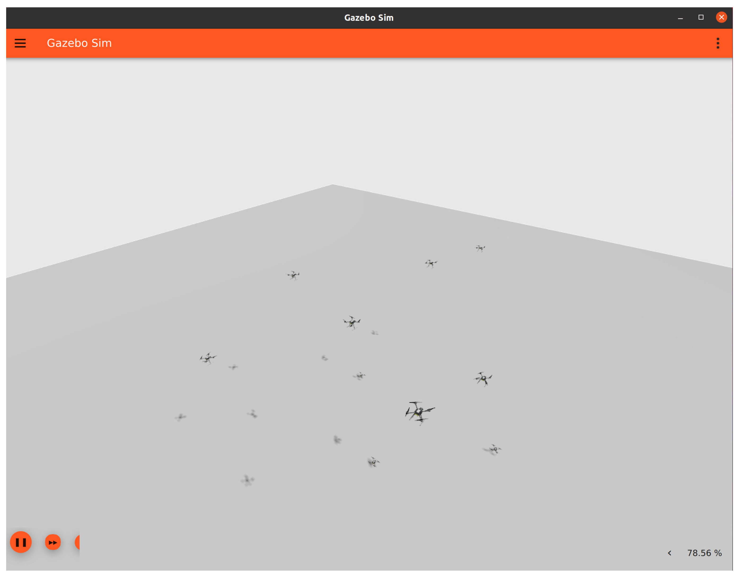
We deployed our model on a Ubuntu 22.04.1 server with 1 NVIDIA GeForce RTX 4090 GPU and 1 AMD Ryzen 9 5950X CPU, and the experiment was conducted in a Python 3.7.10, Pytorch 1.12.1, and CUDA 12.0 environment. Our algorithms can be applied on the Gazebo Garden simulation with drone model gz_x500, as shown in Figure 7, but the training process is too slow because of some limitations of Gazebo simulation. As a result, we trained our algorithms in a grid world as a way to be more efficient.
In our experiments, we used the ERGN as the decision-making agent for UAV mission execution. During the execution of exploration tasks, our agents need to control the UAVs and try to survey more ground areas in the limited time steps. Communication between the UAVs can be established within a certain range; we consider this topological relationship between the UAVs as an adjacency matrix. The UAV’s power situation is defined as a health status vector; our model can accept both adjacency matrics and state vectors to help agents make an action decision. We included the Deep Q Network (DQN) and Deep Graph Network (DGN) as baselines for comparative analysis. The DQN is the baseline for Multi-UAV performance in ground exploration missions without communications, and the DGN is a baseline for communications without fault tolerance. Then, we applied the ERGN to the experiment to examine the difference between it and other algorithms. We designed two sets of experiments for the ERGN: one set is the normal ERGN, and the other set is an advanced ERGN with a time-sequential recurrent neural network—LSTM. Following the experiments, we summarize and discuss the advantages of our proposed algorithms.

2.6. Training Scenarios

In this section, we describe the mission details for the exploration scenario. We designed an exploration scenario with 10 UAVs. The swarm of UAVs needs to explore ground areas with 30 × 30 units. The UAV has a communication range of four units and an explore coverage of one unit. At each time step, the UAV can move one unit in the playground. The more areas explored by the UAVs, the higher the UAV scores. At the beginning of the episode, there are 10 UAVs separated in different locations. Each UAV is randomly initialized with an energy level between 20 and 40. The UAV consumes one unit of energy at each time step. If the UAV runs out of energy, it will drop into a faulty status, and it is immovable. The UAV needs to wait for other companions to rescue it; when another UAV approaches one unit of distance, the faulty one is considered to be successfully rescued, and the successful rescue UAV will recover 20 energy units to continue the mission. Each episode consists of 200 time steps.

3. Results and Discussion

In this section, experiments have been conducted on the ERGN algorithm proposed above to test its efficiency in Multi-UAV exploration missions. Then, we compare with the baseline algorithm to evaluate the performance of the algorithm. These items are included in the analysis list, including reward convergence, the number of areas explored, and the number of rescue occurrences.
In the experiments, we chose the DQN as the baseline and tested the performance of the ERGN. The experimental results indicate that our algorithms had better performance in the task. As shown in Figure 8 through the convergence of the reward curves, it can be seen that the new algorithm exhibited better performance improvement.
We recorded the reward index every 20 episodes in the experiments; the result shows that the DQN algorithm converged at the level of −100 points, and the DGN algorithm converged at the level of −60 points. After that, our ERGN algorithm converged to the level of −50 with the help of fault tolerance. At the same time, the convergence was faster, and the convergence process was as stable as other algorithms. Beyond that, we integrated the LSTM temporal memory into the ERGN, and the performance was better. We can find the result in the Figure 8. The ERGN algorithm with LSTM achieved a higher level, about −40 points. What is more, the convergence process was much faster. Moreover, at 4000 episodes, the reward temporarily exceeded the level of −40 points. It was stronger than the ERGN alone and significantly better than the DQN and DGN.
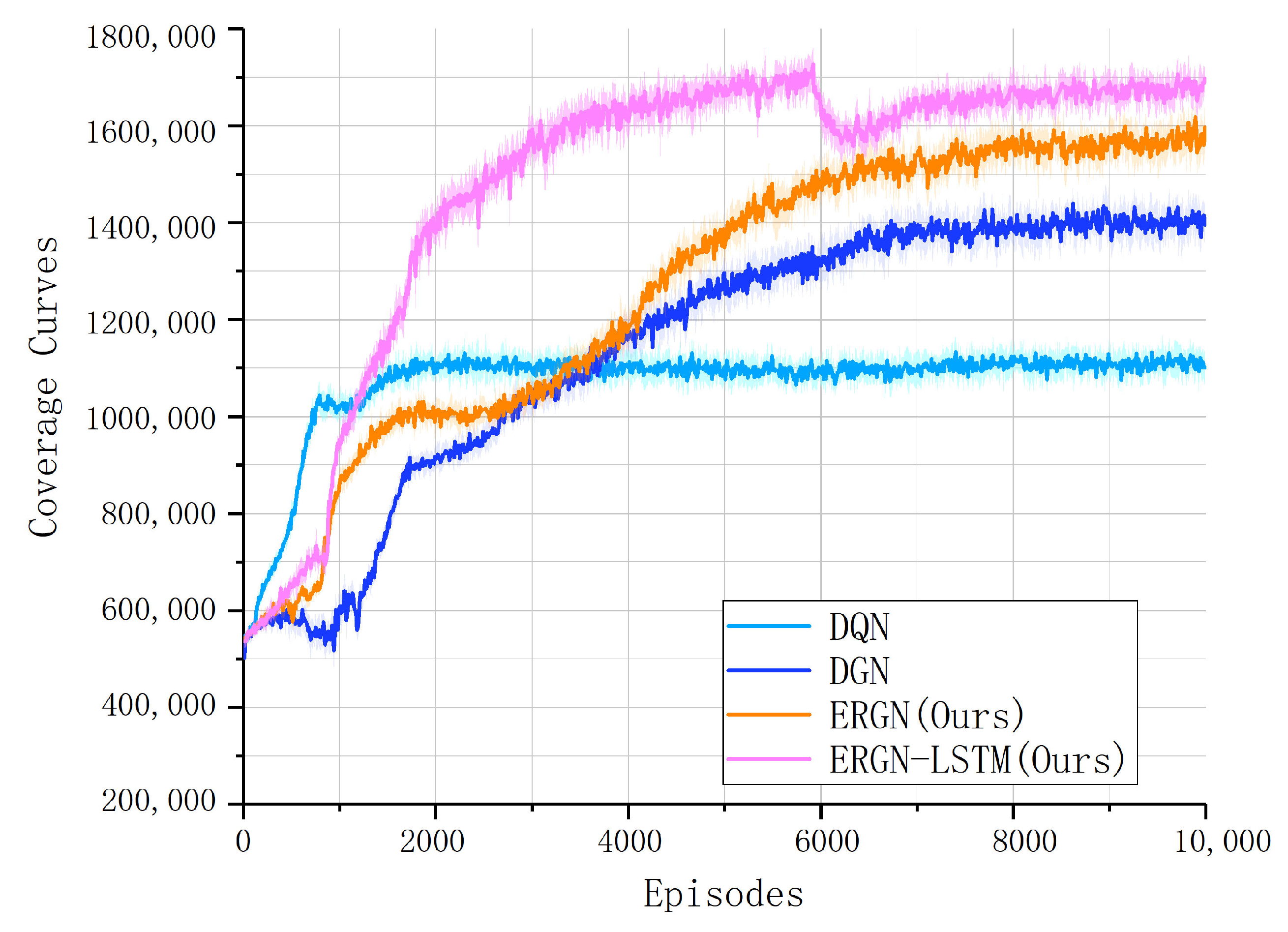
We recorded the coverage index during the experience every 20 episodes; it can reflect the number of explored areas in the real missions. Figure 9 depicts the coverage indexes. We can find from Figure 8 and Figure 9 that the exploration coverage of the UAV swarms expanded as training progressed, and the agents gradually learned to cooperate to explore more areas in the limited time steps. The change in coverage curves during training was consistent with the reward curves, which confirms the effectiveness of the training process. The best algorithm was the ERGN-LSTM, because it had the highest reward and coverage index, and the second one was the ERGN; following them were the DGN and DQN. This indicates that the collaborative approach of our self-organized rescue group plays a certain role in the joint exploration mission of UAVs. This indicates that our algorithm is effective in the exploration tasks.
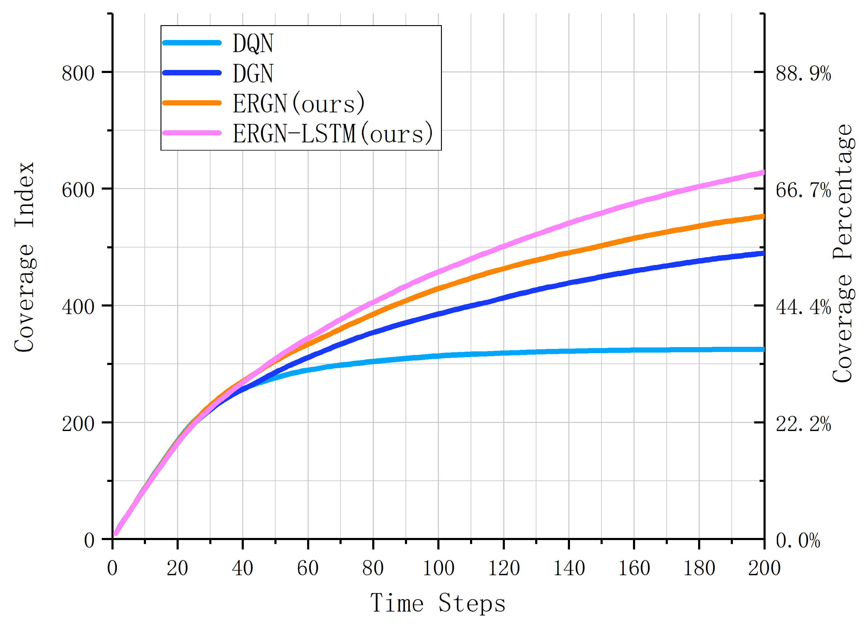
In order to find out the exploration process over time, we conducted 100 repeated experiments with the trained model and took the averages to view the exploration process of the UAV swarm. Figure 10 shows the result of the experiments. Over 200 time steps, the exploration area of the UAV swarm continuously expanded. We can find that the DQN algorithm reached its maximum exploration ranges at 60 time steps, or about 300 units of area. The DGN had a better performance, thus reaching a level of 500 units of area, but the curve was relatively flat, with little potential. The ERGN algorithm could reach a level of about 550 unit areas when proceeding to 200 time steps. The ERGN-LSTM algorithm expanded continuously and reached a unit level of 600 unit areas in the end. The score was continuously expanding, and more time steps would have had a greater exploration potential. The curve of the ERGN-LSTM rose rapidly, which indicates that it has greater potential.
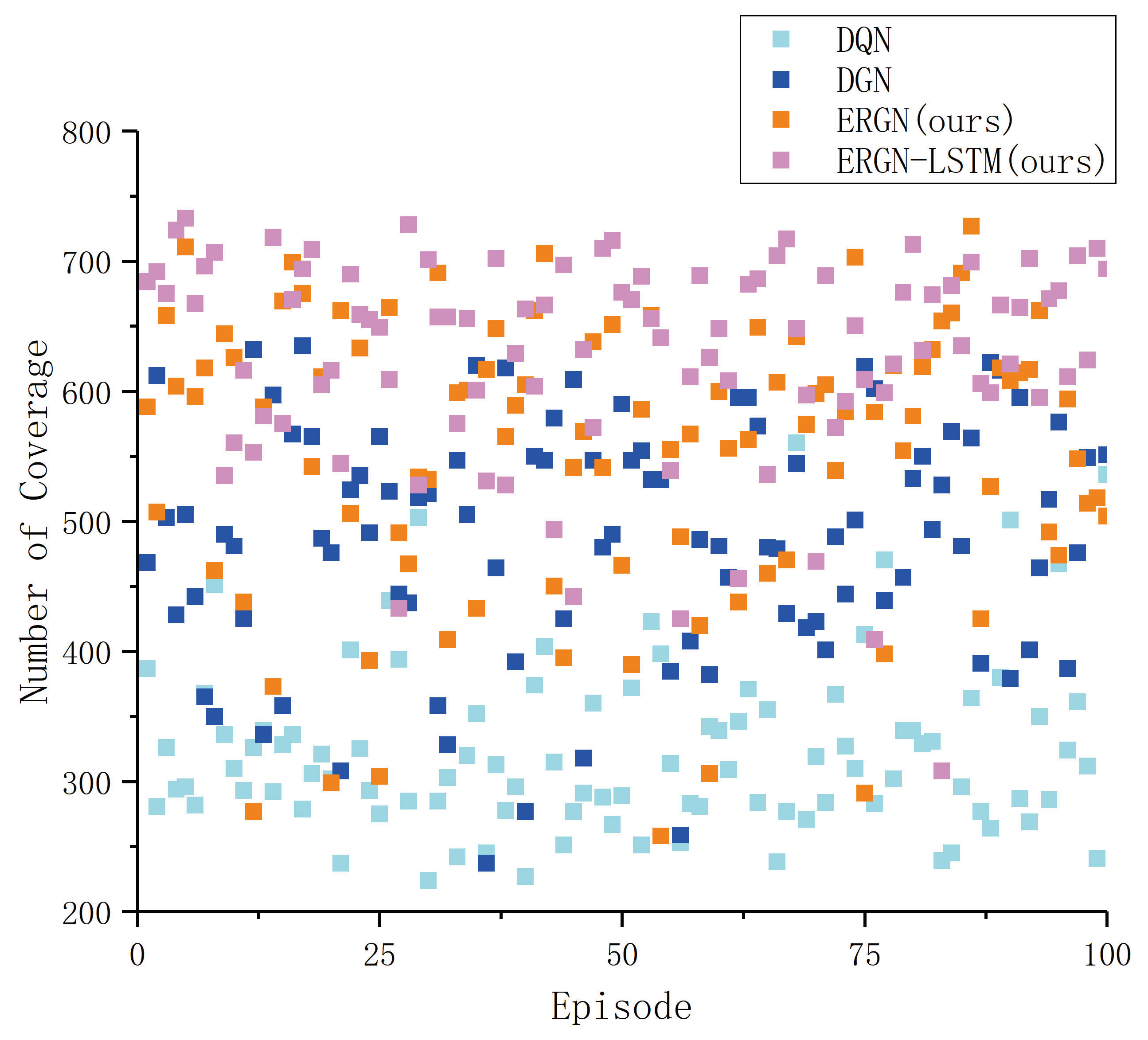
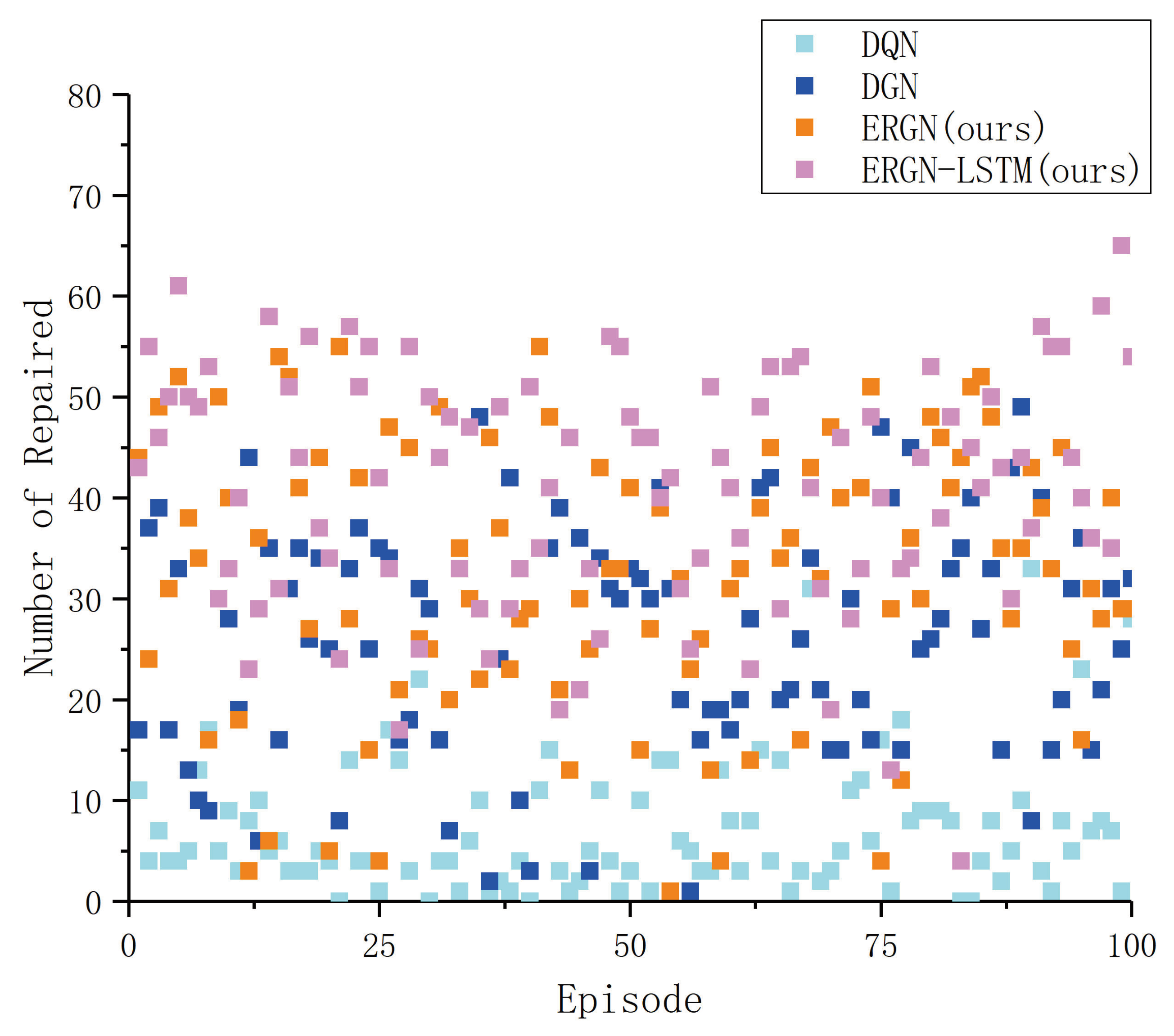
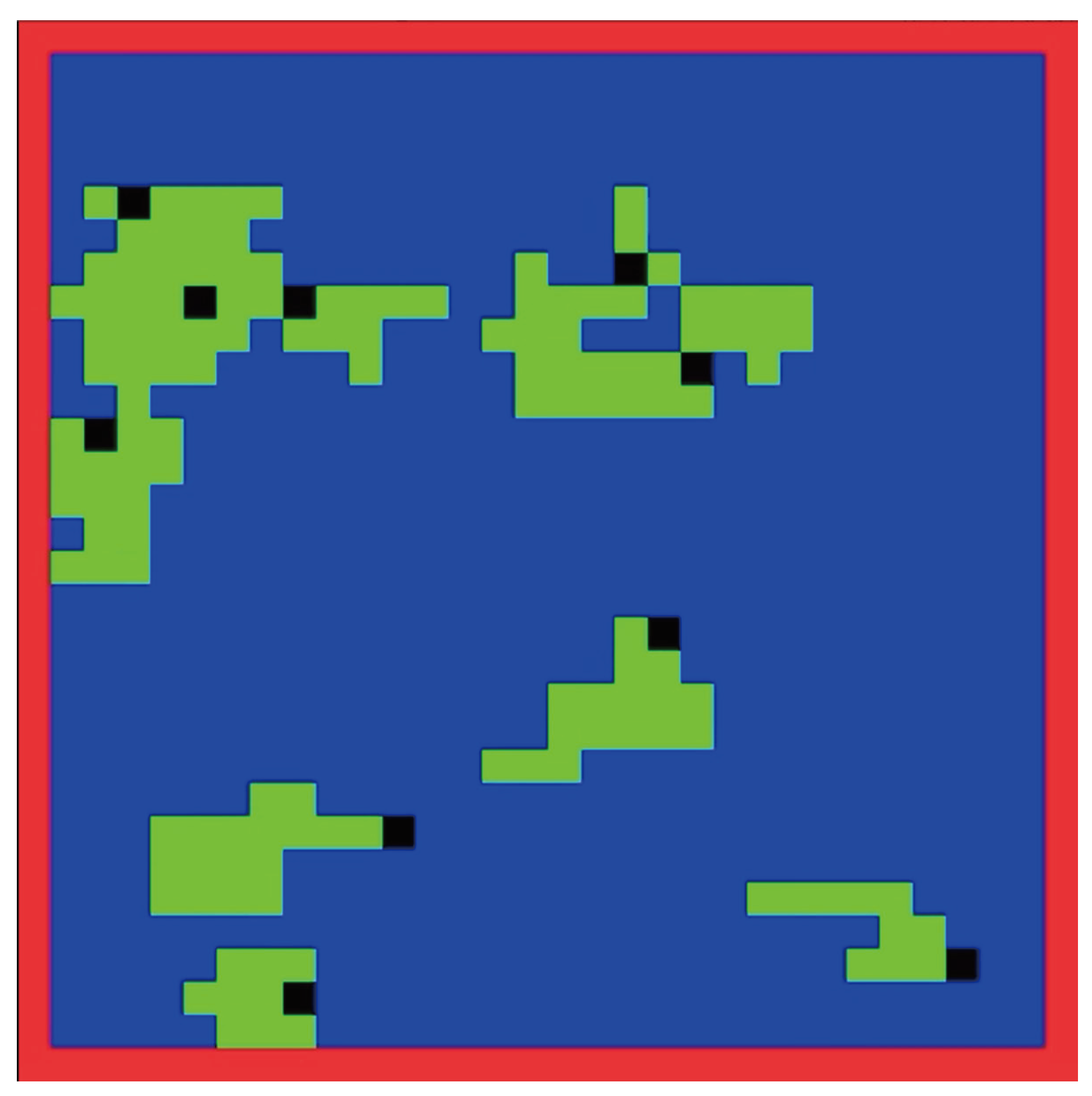
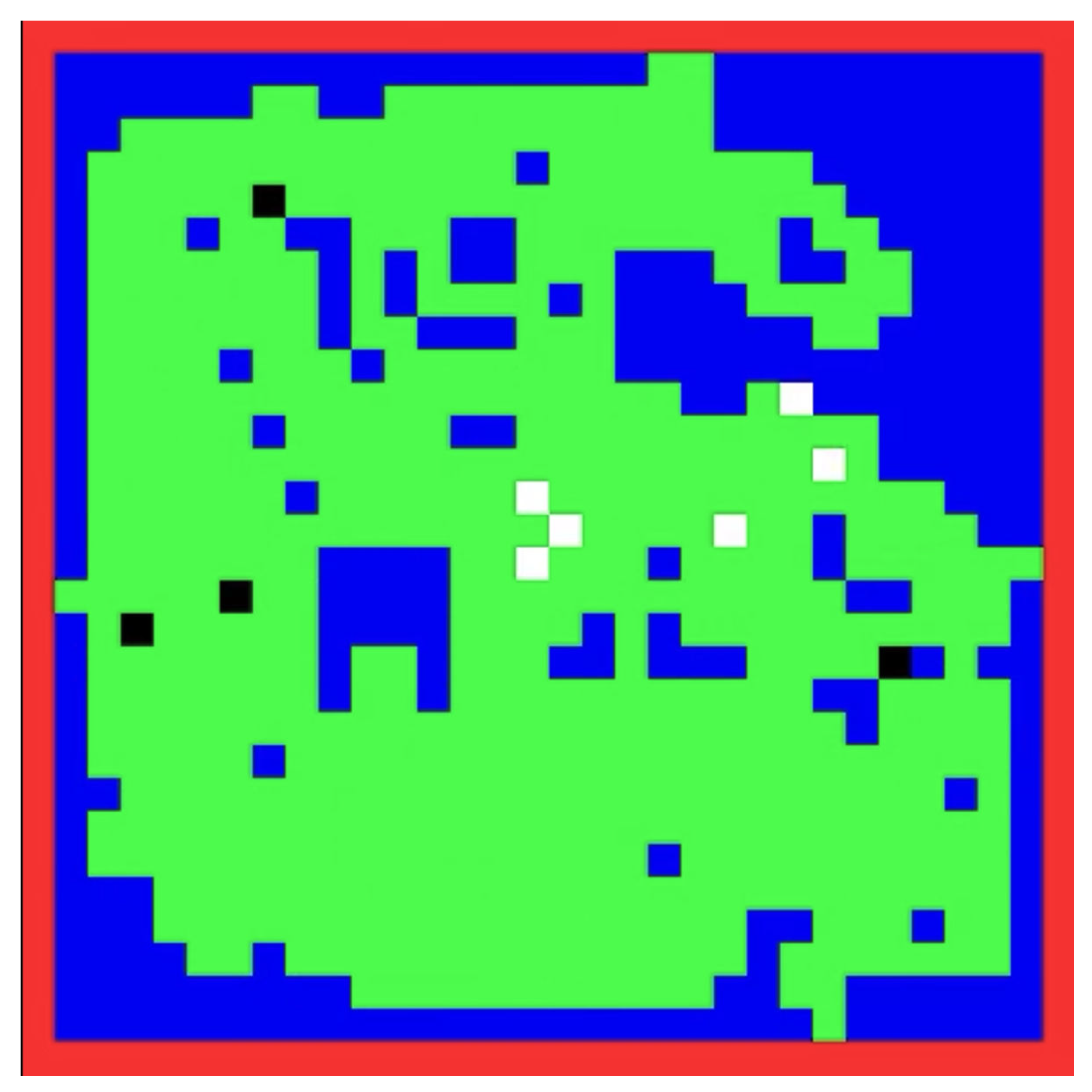
The following figures (Figure 11 and Figure 12) represent the number of exploration areas and the number of repaired UAVs in these 100 experiments. The ERGN-LSTM model could schedule the UAVs to reach a level of approximately 600 units of exploration areas, show as Figure 13 and Figure 14; the scores may have varied depending on the initial position and health status of the UAVs. The DQN model could only maintain the exploration level at around 300 units of areas. The performance of the other algorithms fell between these two extremes. We can find that there is a strong relationship between the number of exploration areas and the number of repaired UAVs through Figure 11 and Figure 12. Models with high rescue rates for faulty UAVs have correspondingly higher exploration efficiencies. In the DQN model, the number of repaired UAVs numbered less than 10 in an episode, whereas our proposed ERGN-LSTM algorithm could reach more than 50 in an episode or even higher. This result is consistent with our intuition that the higher the number of surviving agents, the higher the level of exploration. The performance of the algorithm is correlated with the initialization of the scenario.
In the future, we also need to enhance the robustness of the algorithms. In our algorithms, the initial positions of the drones will influence the efficiency of cooperation and affect the performance of the algorithms. We initialized the agent positions randomly, and the performance of the algorithm fluctuates when the agents initiate in different positions. We are trying to optimize these problems. Overall, our algorithms have a better performance compared with the DQN and other normal algorithms when the faulty agents appear in the playground. In exploration missions, it can help the agents learn to cooperate and go to rescue the faulty agent; they can maintain the ability of swarm and achieve beautiful performance.

4. Conclusions

In this paper, we designed an algorithm called the ERGN. The ERGN can manage UAVs in different states during explore missions. It can schedule the swarm toward the mission target. We verified the performance of our algorithm in the scenario of Multi-UAV exploration. After the training process, our algorithm learned to control the UAV swarm; it could overcome the difficulties posed by faulty UAVs and dispatch the UAVs toward the mission target. The UAVs learned to work together and support assistance when a partner met a breakdown. We also integrated the temporal module to enhance the performance of the ERGN. Our algorithm shows a clear improvement in the exploration task compared to traditional algorithms.

Author Contributions

Conceptualization, Z.J. and G.S.; methodology, Z.J.; software, Z.J.; validation, Z.J. and G.S.; formal analysis, Z.J.; investigation, Z.J.; resources, G.S.; data curation, Z.J.; writing—original draft preparation, Z.J. and T.S.; writing—review and editing, Z.J., B.Y. and G.S.; visualization, Z.J. and T.S.; supervision, G.S.; project administration, G.S.; funding acquisition, G.S. All authors have read and agreed to the published version of the manuscript.

Funding

This research was funded by the National Natural Science Foundation of China under Grant No. 62236007.

Data Availability Statement

The raw data supporting the conclusions of this article will be made available by the authors on request.

Conflicts of Interest

The authors declare no conflicts of interest.

Abbreviations

The following abbreviations are used in this manuscript:
MARLMulti-Agent Reinforcement Learning
UAVUnmanned Aerial Vehicle
DQNDeep Q Network
DGNDeep Graph Network
ERGNError-Resilient Graph Network
GATsGraph Attention Networks
LSTMLong Short-Term Memory
MLPMulti-Layer Perceptron

References

  1. Fan, B.; Li, Y.; Zhang, R.; Fu, Q. Review on the technological development and application of UAV systems. Chin. J. Electron. 2020, 29, 199–207. [Google Scholar] [CrossRef]
  2. Ravankar, A.A.; Ravankar, A.; Kobayashi, Y.; Emaru, T. Autonomous mapping and exploration with unmanned aerial vehicles using low cost sensors. Multidiscip. Digit. Publ. Inst. Proc. 2018, 4, 44. [Google Scholar]
  3. Zhou, B.; Xu, H.; Shen, S. Racer: Rapid collaborative exploration with a decentralized multi-uav system. IEEE Trans. Robot. 2023, 39, 1816–1835. [Google Scholar] [CrossRef]
  4. Jiang, Z.; Chen, Y.; Wang, K.; Yang, B.; Song, G. A Graph-Based PPO Approach in Multi-UAV Navigation for Communication Coverage. Int. J. Comput. Commun. Control 2023, 18, 5505. [Google Scholar] [CrossRef]
  5. Jiang, Z.; Chen, Y.; Song, G.; Yang, B.; Jiang, X. Cooperative planning of multi-UAV logistics delivery by multi-graph reinforcement learning. In Proceedings of the International Conference on Computer Application and Information Security (ICCAIS 2022), Wuhan, China, 23–24 December 2022; Volume 12609, pp. 129–137. [Google Scholar]
  6. Zhan, G.; Zhang, X.; Li, Z.; Xu, L.; Zhou, D.; Yang, Z. Multiple-uav reinforcement learning algorithm based on improved ppo in ray framework. Drones 2022, 6, 166. [Google Scholar] [CrossRef]
  7. Rezaee, H.; Parisini, T.; Polycarpou, M.M. Almost sure resilient consensus under stochastic interaction: Links failure and noisy channels. IEEE Trans. Autom. Control 2020, 66, 5727–5741. [Google Scholar] [CrossRef]
  8. Jiang, H.; Shi, D.; Xue, C.; Wang, Y.; Wang, G.; Zhang, Y. Multi-agent deep reinforcement learning with type-based hierarchical group communication. Appl. Intell. 2021, 51, 5793–5808. [Google Scholar] [CrossRef]
  9. Mann, V.; Sivaram, A.; Das, L.; Venkatasubramanian, V. Robust and efficient swarm communication topologies for hostile environments. Swarm Evol. Comput. 2021, 62, 100848. [Google Scholar] [CrossRef]
  10. Gu, S.; Geng, M.; Lan, L. Attention-based fault-tolerant approach for multi-agent reinforcement learning systems. Entropy 2021, 23, 1133. [Google Scholar] [CrossRef]
  11. Xing, Z.; Jia, J.; Guo, K.; Jia, W.; Yu, X. Fast active fault-tolerant control for a quadrotor uav against multiple actuator faults. Guid. Navig. Control 2022, 2, 2250007. [Google Scholar] [CrossRef]
  12. Muslimov, T. Adaptation Strategy for a Distributed Autonomous UAV Formation in Case of Aircraft Loss. In Proceedings of the International Symposium on Distributed Autonomous Robotic Systems, Montbéliard, France, 28–30 November 2022; pp. 231–242. [Google Scholar]
  13. Bianchi, D.; Di Gennaro, S.; Di Ferdinando, M.; Acosta Lùa, C. Robust control of uav with disturbances and uncertainty estimation. Machines 2023, 11, 352. [Google Scholar] [CrossRef]
  14. Kilinc, O.; Montana, G. Multi-agent deep reinforcement learning with extremely noisy observations. arXiv 2018, arXiv:1812.00922. [Google Scholar]
  15. Luo, C.; Liu, X.; Chen, X.; Luo, J. Multi-agent Fault-tolerant Reinforcement Learning with Noisy Environments. In Proceedings of the 2020 IEEE 26th International Conference on Parallel and Distributed Systems (ICPADS), Hong Kong, China, 2–4 December 2020; pp. 164–171. [Google Scholar]
  16. Abel, R.O.; Dasgupta, S.; Kuhl, J.G. The relation between redundancy and convergence rate in distributed multi-agent formation control. In Proceedings of the 2008 47th IEEE Conference on Decision and Control, Cancun, Mexico, 9–11 December 2008; pp. 3977–3982. [Google Scholar]
  17. Wang, G.; Luo, H.; Hu, X.; Ma, H.; Yang, S. Fault-tolerant communication topology management based on minimum cost arborescence for leader–follower UAV formation under communication faults. Int. J. Adv. Robot. Syst. 2017, 14, 1729881417693965. [Google Scholar] [CrossRef]
  18. Han, B.; Jiang, J.; Yu, C. Distributed fault-tolerant formation control for multiple unmanned aerial vehicles under actuator fault and intermittent communication interrupt. Proc. Inst. Mech. Eng. Part I J. Syst. Control Eng. 2021, 235, 1064–1083. [Google Scholar] [CrossRef]
  19. Hu, J.; Niu, H.; Carrasco, J.; Lennox, B.; Arvin, F. Fault-tolerant cooperative navigation of networked UAV swarms for forest fire monitoring. Aerosp. Sci. Technol. 2022, 123, 107494. [Google Scholar] [CrossRef]
  20. Ghamry, K.A.; Zhang, Y. Fault-tolerant cooperative control of multiple UAVs for forest fire detection and tracking mission. In Proceedings of the 2016 3rd Conference on Control and Fault-Tolerant Systems (SysTol), Barcelona, Spain, 7–9 September 2016; pp. 133–138. [Google Scholar]
  21. Huang, S.; Teo, R.S.H.; Kwan, J.L.P.; Liu, W.; Dymkou, S.M. Distributed UAV loss detection and auto-replacement protocol with guaranteed properties. J. Intell. Robot. Syst. 2019, 93, 303–316. [Google Scholar] [CrossRef]
  22. Oroojlooy, A.; Hajinezhad, D. A review of cooperative multi-agent deep reinforcement learning. Appl. Intell. 2023, 53, 13677–13722. [Google Scholar] [CrossRef]
  23. Kim, W.; Park, J.; Sung, Y. Communication in multi-agent reinforcement learning: Intention sharing. In Proceedings of the International Conference on Learning Representations, Addis Ababa, Ethiopia, 30 April 2020. [Google Scholar]
  24. Zhang, K.; Yang, Z.; Başar, T. Multi-agent reinforcement learning: A selective overview of theories and algorithms. In Handbook of Reinforcement Learning and Control; Springer: Berlin/Heidelberg, Germany, 2021; pp. 321–384. [Google Scholar]
  25. Zhang, Y.; Yang, Q.; An, D.; Zhang, C. Coordination between individual agents in multi-agent reinforcement learning. In Proceedings of the AAAI Conference on Artificial Intelligence, virtually, 2–9 February 2021; Volume 35, pp. 11387–11394. [Google Scholar]
  26. Yu, C.; Velu, A.; Vinitsky, E.; Gao, J.; Wang, Y.; Bayen, A.; Wu, Y. The surprising effectiveness of ppo in cooperative multi-agent games. Adv. Neural Inf. Process. Syst. 2022, 35, 24611–24624. [Google Scholar]
  27. Yang, X.; Huang, S.; Sun, Y.; Yang, Y.; Yu, C.; Tu, W.W.; Yang, H.; Wang, Y. Learning Graph-Enhanced Commander-Executor for Multi-Agent Navigation. arXiv 2023, arXiv:2302.04094. [Google Scholar]
  28. Egorov, M. Multi-agent deep reinforcement learning. In CS231n: Convolutional Neural Networks for Visual Recognition; Stanford.edu: Stanford, CA, USA, 2016; pp. 1–8. [Google Scholar]
  29. de Witt, C.S.; Gupta, T.; Makoviichuk, D.; Makoviychuk, V.; Torr, P.H.; Sun, M.; Whiteson, S. Is independent learning all you need in the starcraft multi-agent challenge? arXiv 2020, arXiv:2011.09533. [Google Scholar]
  30. Tan, M. Multi-agent reinforcement learning: Independent vs. cooperative agents. In Proceedings of the Tenth International Conference on Machine Learning, Amherst, MA, USA, 27–29 June 1993; pp. 330–337. [Google Scholar]
  31. Chu, X.; Ye, H. Parameter sharing deep deterministic policy gradient for cooperative multi-agent reinforcement learning. arXiv 2017, arXiv:1710.00336. [Google Scholar]
  32. Brody, S.; Alon, U.; Yahav, E. How attentive are graph attention networks? arXiv 2021, arXiv:2105.14491. [Google Scholar]
  33. Liu, Y.; Wang, W.; Hu, Y.; Hao, J.; Chen, X.; Gao, Y. Multi-agent game abstraction via graph attention neural network. In Proceedings of the AAAI Conference on Artificial Intelligence, New York, NY, USA, 7–12 February 2020; Volume 34, pp. 7211–7218. [Google Scholar]
  34. Hamilton, W.; Ying, Z.; Leskovec, J. Inductive representation learning on large graphs. Adv. Neural Inf. Process. Syst. 2017, 30, 1025–1035. [Google Scholar]
  35. Mnih, V.; Kavukcuoglu, K.; Silver, D.; Rusu, A.A.; Veness, J.; Bellemare, M.G.; Graves, A.; Riedmiller, M.; Fidjeland, A.K.; Ostrovski, G.; et al. Human-level control through deep reinforcement learning. Nature 2015, 518, 529–533. [Google Scholar] [CrossRef] [PubMed]
  36. Veličković, P.; Cucurull, G.; Casanova, A.; Romero, A.; Lio, P.; Bengio, Y. Graph attention networks. arXiv 2017, arXiv:1710.10903. [Google Scholar]
  37. Shi, X.; Chen, Z.; Wang, H.; Yeung, D.Y.; Wong, W.K.; Woo, W.c. Convolutional LSTM network: A machine learning approach for precipitation nowcasting. Adv. Neural Inf. Process. Syst. 2015, 28. [Google Scholar]
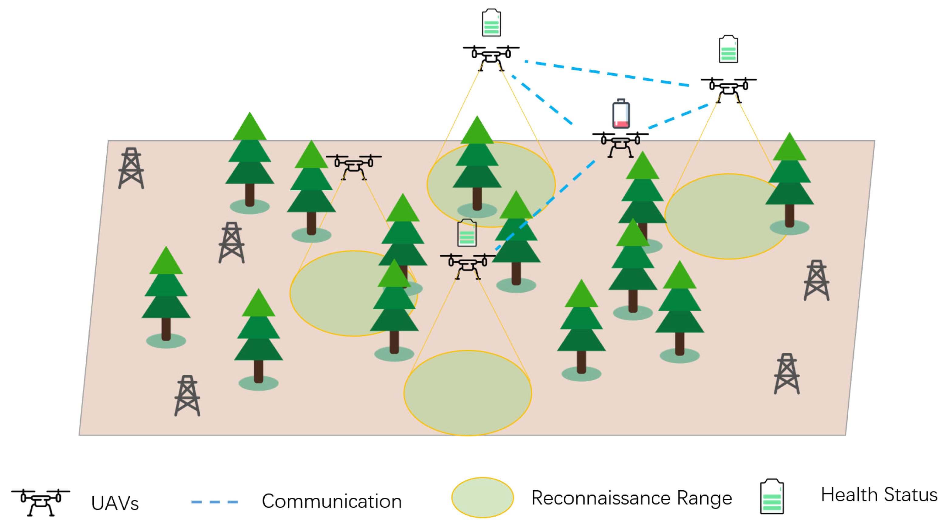
Figure 1. The task of Multi-UAV ground exploration.
Aerospace 11 00372 g001
Figure 2. The framework of ERGN.
Aerospace 11 00372 g002
Figure 3. Graph Aggregator.
Aerospace 11 00372 g003
Figure 4. Formation of rescue groups.
Aerospace 11 00372 g004
Figure 5. Policy network.
Aerospace 11 00372 g005
Figure 6. Policy network training process.
Aerospace 11 00372 g006
Figure 7. Gazebo Garden simulation with ROS2.
Aerospace 11 00372 g007
Figure 8. Reward curves.
Aerospace 11 00372 g008
Figure 9. Coverage curves.
Aerospace 11 00372 g009
Figure 10. Coverage with time step.
Aerospace 11 00372 g010
Figure 11. Coverage with episode.
Aerospace 11 00372 g011
Figure 12. Repaired drones with episode.
Aerospace 11 00372 g012
Figure 13. Performance before training.
Aerospace 11 00372 g013
Figure 14. Performance after training.
Aerospace 11 00372 g014
Disclaimer/Publisher’s Note: The statements, opinions and data contained in all publications are solely those of the individual author(s) and contributor(s) and not of MDPI and/or the editor(s). MDPI and/or the editor(s) disclaim responsibility for any injury to people or property resulting from any ideas, methods, instructions or products referred to in the content.