Article

A Short-Term Traffic Flow Prediction Method for Airport Group Route Waypoints Based on the Spatiotemporal Features of Traffic Flow

1
College of Civil Aviation, Nanjing University of Aeronautics and Astronautics, Nanjing 211106, China
2
State Key Laboratory of Air Traffic Management System, Nanjing 211106, China
3
College of General Aviation and Flight, Nanjing University of Aeronautics and Astronautics, Nanjing 211106, China
4
College of Computer Science and Technology, Nanjing University of Aeronautics and Astronautics, Nanjing 211106, China
5
The Second Research Institute of CAAC, Chengdu 610041, China
*
Author to whom correspondence should be addressed.
Aerospace 2024, 11(4), 248; https://doi.org/10.3390/aerospace11040248
Submission received: 3 February 2024 / Revised: 9 March 2024 / Accepted: 21 March 2024 / Published: 22 March 2024

Abstract

:
To fully leverage the spatiotemporal dynamic correlations in air traffic flow and enhance the accuracy of traffic flow prediction models, thereby providing a more precise basis for perceiving congestion situations in the air route network, a study was conducted on a traffic flow prediction method based on deep learning considering spatiotemporal factors. A waypoint network topology graph was constructed, and a neural network model called graph convolution and self-attention-based long short-term memory neural network (GC-SALSTM) was proposed. This model utilized waypoint flow and network efficiency loss rate as input features, with graph convolution extracting spatial features from the waypoint network. Additionally, a long short-term memory network based on a self-attention mechanism was used to extract temporal features, achieving accurate prediction of waypoint traffic. An example analysis was performed on a typical busy sector of airports in the Central and Southern China region. The effectiveness of adding the network efficiency loss rate as an input feature to improve the accuracy of critical waypoint traffic prediction was validated. The performance of the proposed model was compared with various typical prediction models. The results indicated that, with the addition of the network efficiency loss rate, the root mean square error (RMSE) for eight waypoints decreased by more than 10%. Compared to the historical average (HA), autoregressive integrated moving average (ARIMA), support vector regression (SVR), long short-term memory (LSTM), and graph convolution network and long short-term memory network (GCN-LSTM) models, the RMSE of the proposed model decreased by 11.78%, 5.55%, 0.29%, 2.53%, and 1.09%, respectively. This suggests that the adopted network efficiency loss rate indicator effectively enhances prediction accuracy, and the constructed model exhibits superior predictive performance in short-term waypoint traffic forecasting compared to other prediction models. It contributes to optimizing flight paths and high-altitude air routes, minimizing flight delays and airborne congestion to the greatest extent, thus enhancing the overall efficiency of the entire aviation system.

1. Introduction

To adapt to the construction and development of world-class airport groups in China and meet the rapid growth in aviation transport demand within the airport group, the structural layout and operational modes of the route network under the jurisdiction of the airport group have become increasingly complex. As time progresses, the strong coupling and correlation among multiple traffic flows running between various waypoints become evident, leading to spatial-temporal cascading reactions that extend to larger scales. This results in a complex and variable operational situation, making it difficult to grasp short-term changes in traffic flow patterns. Consequently, sudden capacity and flow imbalances occur frequently, posing significant safety risks on the airspace operation of the airport group. Accurate exploration of congestion patterns in the airport group requires urgent attention. To gain a scientific understanding of the sudden changes in capacity and flow imbalances at various waypoints within the group, it is crucial to study the spatiotemporal characteristics of traffic data at specific waypoints within an airport group. This research aims to develop short-term forecasting methods for traffic flow at waypoints within an airport group.
Currently, research on air traffic flow forecasting both domestically and internationally is mainly focused on two aspects. Firstly, it involves predicting traffic flow based on the four-dimensional trajectories of aircraft, targeting different airspace units such as waypoints, air segments, sectors, and airports. This is primarily carried out using flight plan data and employing trajectory matching algorithms, adaptive trajectory clustering algorithms, planned trajectory, and radar trajectory matching and correlation algorithms. These methods perform four-dimensional trajectory prediction and forecast traffic flow in airspace units [1,2,3]. Secondly, it relies on statistical analysis of historical traffic data for different airspace units such as waypoints, air segments, sectors, and airports. This includes classical models primarily based on historical average (HA) model, autoregressive integrated moving average (ARIMA) model, machine learning methods dominated by support vector machines (SVM) [4], and deep learning methods that perform better in multidimensional data processing and spatiotemporal feature extraction [5,6]. These deep learning methods utilize various models such as T-GCN [7], STS-DGCN [8], Location-GCN [9], AFMSTGCN [10], DGC-GRU [11], Bi-AGGCN [12], ConvLSTM [13], SCLN-TTF [14], AG2S-Net [15], AAGC-GRU [16], improved Cao method [17], ATFPNet [18], etc. By considering issues, such as spatiotemporal dynamic correlation mining of traffic flow [19] and external factors (weather [20], holidays), these methods construct congestion indices [21], delay indices [22], and employ various techniques to predict traffic flow [23] and congestion indices.
In traditional research, the focus has primarily been on different spatial units, predicting traffic by individual aircraft trajectories or statistical analysis of historical data. However, superior deep learning methods target a broader spatial domain, including airspace grids, route networks, and airport networks. These methods, based on indicators like flight delays and congestion indices, often overlook the inherent complex network characteristics of airport group systems and the spatial correlations of traffic flow with distance at route points. Additionally, they tend to neglect the similarity in traffic flow characteristics of non-adjacent but functionally similar route points. In light of this, our study focuses on route points in typical busy sectors within airport groups. Considering the spatiotemporal features and correlations of traffic flow at each route point, we selected traffic flow and network efficiency loss rate as indicators. We constructed a short-term traffic flow prediction model based on the GC-SALSTM model. The method was validated and analyzed using route points in typical sectors of the airport group airspace system in the Central and Southern China region. The research findings can contribute to ensuring the safe operation of large busy airport group airspace, improving short-term traffic flow prediction capabilities, and reducing scattered sudden imbalances in capacity and flow.
The remaining sections of the paper are organized as follows: Section 2 provides an analysis of the spatiotemporal features of air traffic flow at waypoints, covering aspects such as the construction of network topology, spatiotemporal feature analysis, and selection of indicators. Section 3 introduces the research methodology, starting with the overall framework of the prediction method and its constituent modules. Section 4 demonstrates the implementation of the method using real ADS-B data, presenting a detailed analysis of the impact of different model parameters and input indicators on the prediction of waypoint traffic flow, including a comparison with other prediction models. Finally, Section 5 concludes this paper, offering further discussions on the proposed method and suggesting possible directions for future research.

2. Analysis of Spatiotemporal Characteristics of Traffic Flow at Route Waypoints

2.1. Construction of Topological Structure for Airport Group Route Network

Using flight plan data from a typical busy sector ZGGGAR22 in the Central and Southern region airport group for the period of 1 March to 31 March 2019, a total of 15,267 flight records were analyzed for spatiotemporal traffic flow characteristics. The data includes flight numbers, departure and arrival airports, planned route points, estimated time over (ETO), actual time over (ATO), speeds, altitudes, and other relevant information. Utilizing the ATO of flights from ADS-B data, we compile the actual traffic at each route point. Route points with lower traffic (flow could be skipped) and insufficient data coverage (or a high number of missing ADS-B positions) were excluded, resulting in 15 route points chosen as prediction targets, with their geographic locations shown in Figure 1. This paper adopts the UTC+8 time zone throughout.
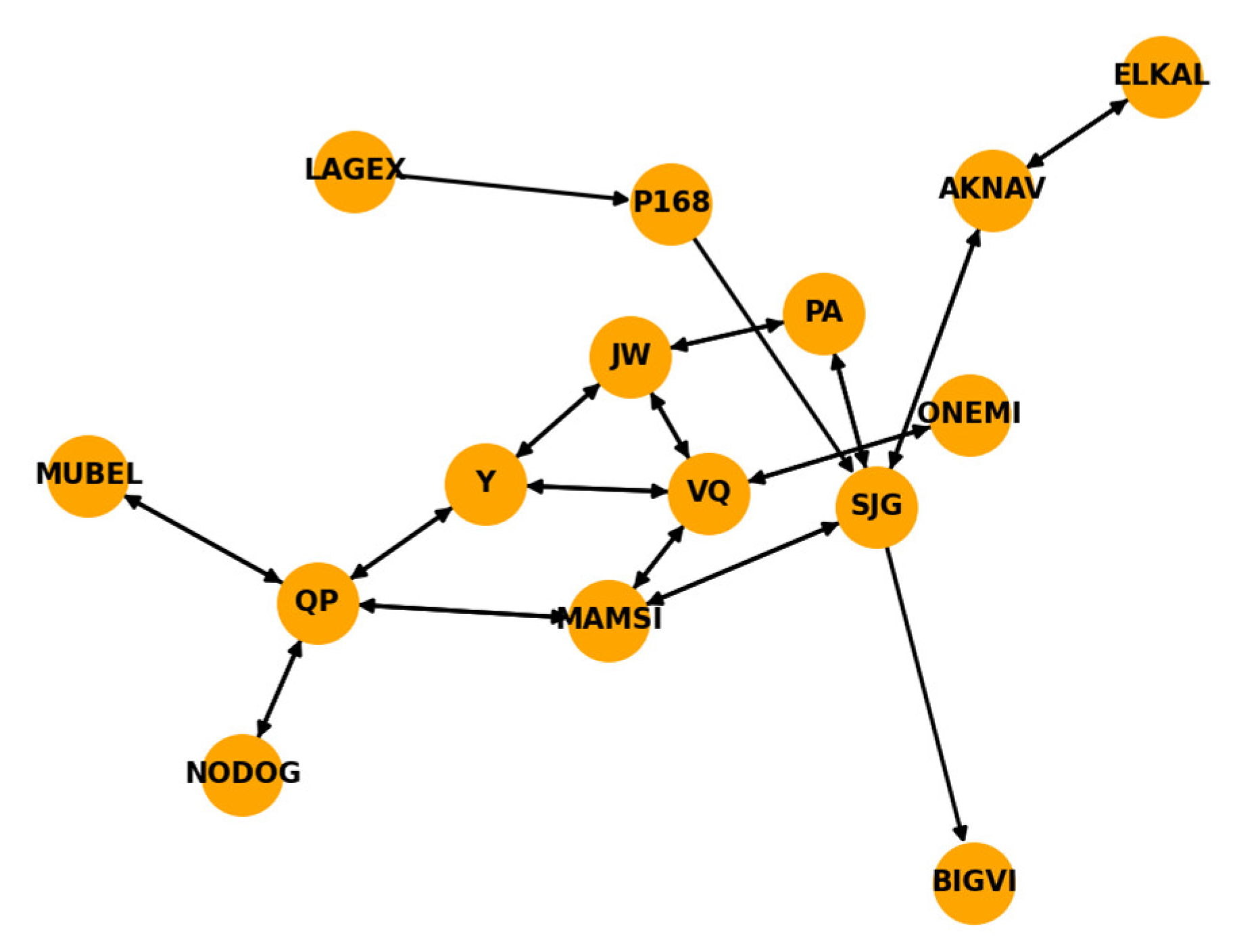
Figure 2 shows a route point network topology structure with 15 route points as nodes and connections (flight segments) between route points as edges. This diagram can be represented as G = ( V , E ) , where V is the set of nodes, denoted as V = { v i | i = 1 , 2 , M } , M represents the number of nodes in the route point network topology diagram G , M = 15 , and E is the set of directed edges, denoted as E = { e i j | i , j = 1 , 2 , , M } .
The adjacency matrix of the route point network topology diagram G is represented as A = ( a i j ) R M × M , where i and j , respectively, represent M nodes. If there is a connection between node i and node j , then a i j = 1 ; otherwise, a i j = 0 .

2.2. Spatiotemporal Analysis of Traffic Flow at Route Waypoints

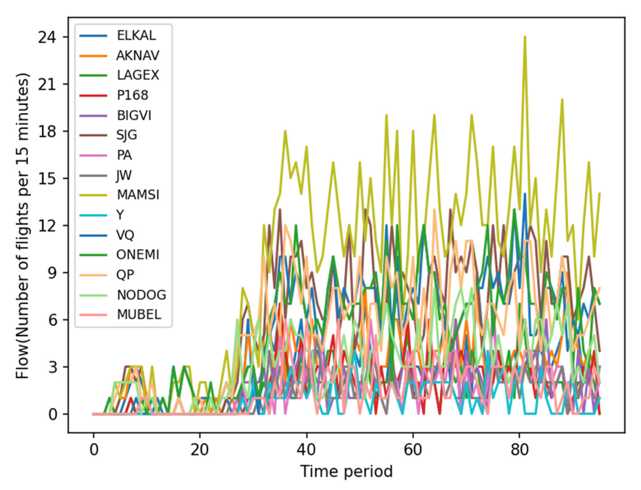
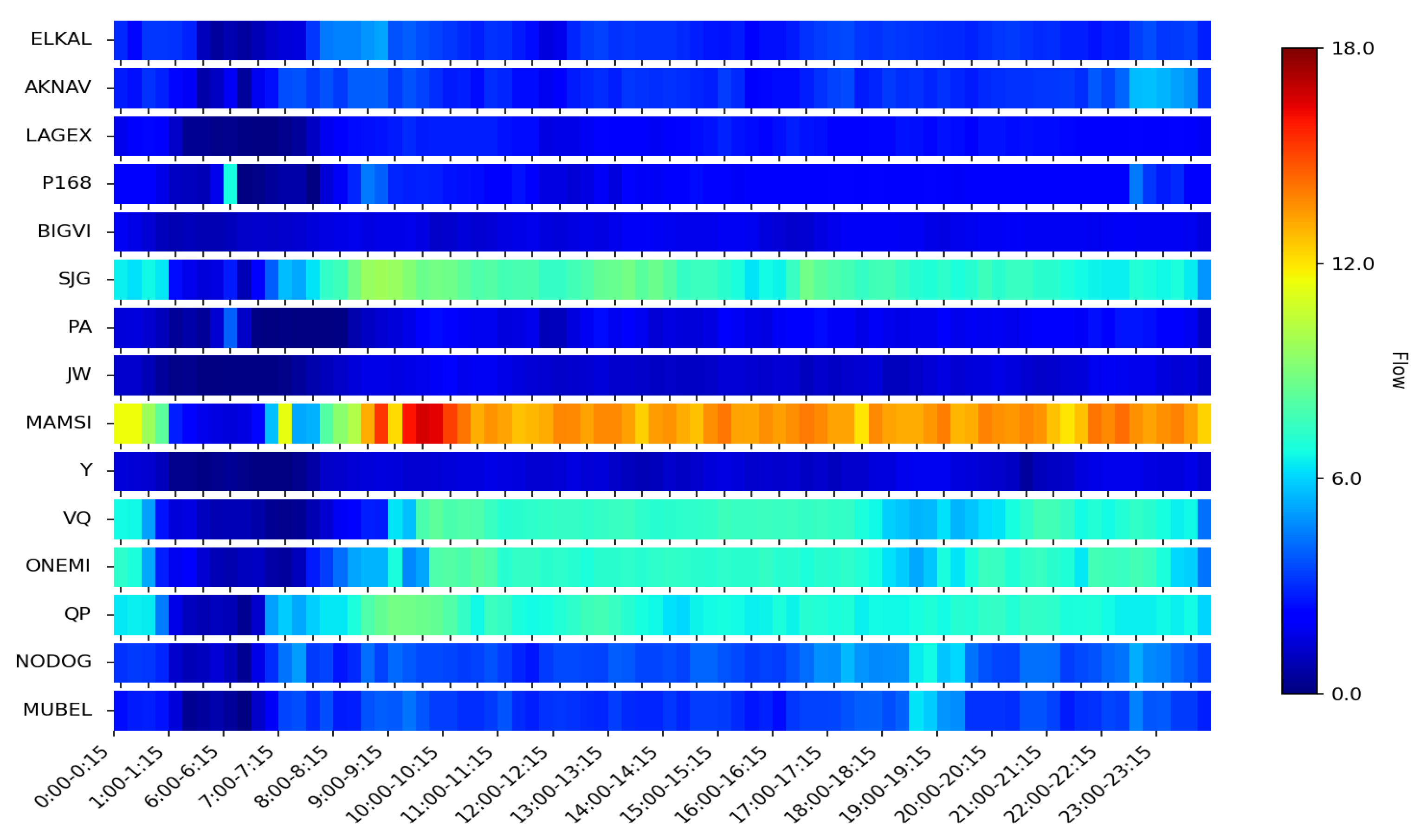
The traffic flow at each route point within the sector comprises the data that possesses both temporal and spatial attributes, displaying significant operational periodicity, spatiotemporal correlations, and other characteristics. To balance time precision and data density, we have chosen a 15 min interval to analyze traffic flow at route points. Figure 3 illustrates the distribution of traffic at 15 route points in sector ZGGGAR22 during typical days, segmented into 15 min intervals. It reveals that, in the temporal dimension, there is a similarity in the trend of traffic variation at different route points throughout the day. In the spatial dimension, significant differences exist in the traffic volume at various route points. Therefore, analyzing the spatiotemporal characteristics of traffic flow at route points is crucial for subsequent traffic predictions. For analysis, MAMSI is selected as it represents the busiest typical route point within the airspace of the Central and Southern region airport group, with nearly a thousand flights passing through daily, involving airports such as Guangzhou, Shenzhen, and Zhuhai.

2.2.1. Temporal Characteristics of Traffic Flow at Route Waypoints

Figure 4 depicts the traffic distribution of MAMSI on every Monday over four consecutive weeks in March 2019. By examining the similarity in traffic on the same day over the four weeks, there is a high degree of resemblance in the Monday traffic trends, indicating a consistent characteristic of periodicity in the traffic distribution every Monday at this route point. By analyzing the traffic variations throughout the day, the traffic distribution at MAMSI exhibits irregular fluctuations and temporal regularities. The irregular fluctuations are characterized by non-smooth variations (not following the expected smooth curve changes) between adjacent time intervals, with unpredictable moments and amplitudes of fluctuation (due to various factors such as weather conditions, airport operational status, etc.). Temporal regularities include traffic decreasing to the daily minimum level between 03:00 and 06:00, a rapid increase from 06:00 to 08:00, maintaining a high level with fluctuations until around 22:00, followed by a continuous decrease until 03:00 the next day.
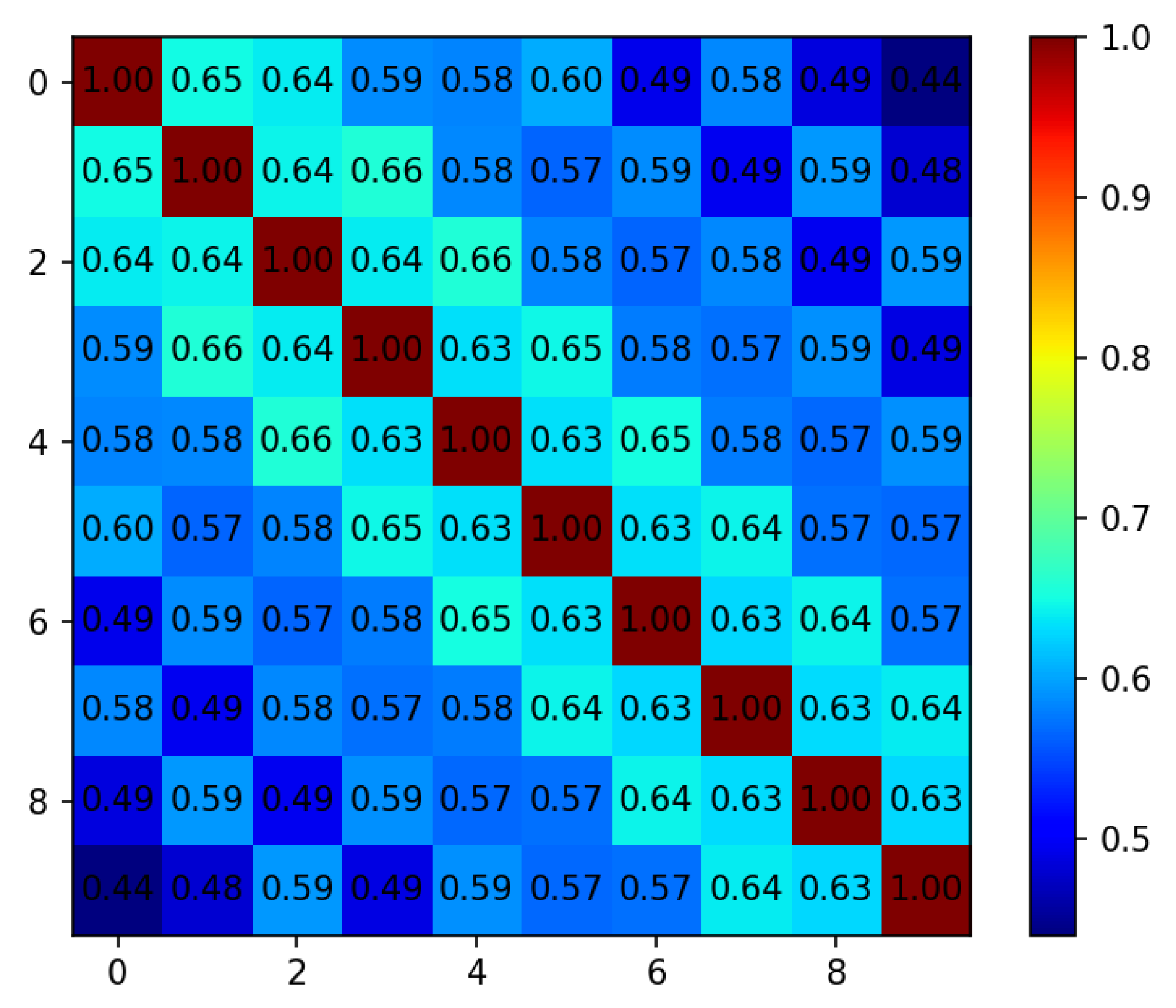
To analyze the correlation of traffic time series at different time intervals for the route point, Pearson’s correlation coefficients [24] were calculated between 10 adjacent time intervals for route point MAMSI, with each time interval spanning 15 min. For instance, when calculating the correlation between the 1st and 2nd time intervals, the two sets of traffic time series data used were X = { f l o w 1 , f l o w 2 , f l o w 96 } and Y = { f l o w 2 , f l o w 3 , f l o w 97 } . The results of the Pearson’s correlation coefficient calculations for the 10 time intervals are shown in Figure 5, indicating a strong correlation between adjacent time intervals. As the distance between time intervals increases, the correlation between traffic time series gradually weakens.

2.2.2. Spatial Characteristics of Traffic Flow at Route Waypoints

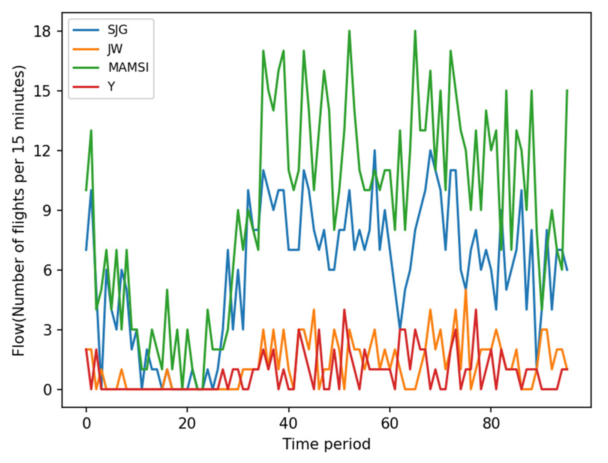
Considering the topological network structure, we selected four typical route points for spatial feature analysis. As shown in Figure 1, the four route points, SJG, MAMSI, JW, and Y, are all located near the geometric center of the sector and serve as crossing points of flight trajectories. They exhibit similarity in their physical spatial distribution. Building upon this, Figure 6 displays the traffic distribution of these four typical route points at various time intervals throughout a typical day. In Figure 6, the traffic distribution at each route point shows spatial variations, indicating differences in traffic volume and trends during different time intervals. For example, the traffic at waypoints SJG and MAMSI is significantly higher than at waypoints JW and Y. However, within these differences, there are also similarities.
We calculate Pearson’s correlation coefficients between traffic flow time series of the 15 route points within the ZGGGAR22 sector for all 96 time intervals throughout the day on 1 March 2019. We select any two waypoints, for instance, ELKAL and AKNAV, and calculate Pearson’s correlation coefficients for the traffic flow time series. The two sets of time series data used for calculation are X = { f l o w 1 E L K A L , f l o w 2 E L K A L , f l o w 96 E L K A L } and Y = { f l o w 1 A K N A V , f l o w 2 A K N A V , f l o w 96 A K N A V } . The results of Pearson’s correlation coefficients for the time series of the 15 route points are shown in Figure 7. In combination with Figure 1, it can be observed that the traffic flow time series of adjacent and directly connected route points exhibit stronger correlation. Additionally, there is a strong correlation between the traffic flow time series of route points that are not directly connected but functionally similar (different locations share similarities in their geographical features, purposes, or services), such as between ELKAL and LAGEX, despite not being directly connected, both serve as sector boundary points. Conversely, route points that are not adjacent and not directly connected tend to have weaker correlations in their traffic flow time series.

2.3. Selection of Spatiotemporal Feature Indicators

It is crucial to judiciously select the spatiotemporal feature indicators for predicting model inputs to enhance prediction accuracy. In addition to historical route point traffic, this study incorporates the route point network efficiency loss rate, a metric commonly used to gauge the importance of nodes in complex networks [25]. While historical traffic reflects temporal characteristics, the route point network adjacency matrix only considers spatial connections between route points, neglecting factors such as the length of segments connecting route points and their impact on spatial correlations of route point traffic. Therefore, this study augments the input indicators with the route point network efficiency loss rate, aiming to comprehensively incorporate spatial features of the route point network into the model. This approach aims to improve prediction accuracy, particularly for crucial bottleneck route points.

2.3.1. Traffic Flow at Route Waypoints

Route point traffic flow refers to the number of flights passing through a specific route point within a given statistical time, reflecting the traffic load at that route point. Commonly used time intervals for traffic statistics include 15 min, 30 min, and 60 min. In this context, the actual traffic flow at each route point within a 15 min interval is denoted as f .

2.3.2. Network Efficiency Loss Rate

The network efficiency loss rate is a metric used to assess the importance of node i in a network and is expressed as follows:
E i l o s s = E E i r e m a i n E
where E is the initial network efficiency, E i r e m a i n is the remaining network efficiency after removing node i and its edges, and E i l o s s is the network efficiency loss rate after removing node i . A higher network efficiency loss rate for node i indicates greater importance of the node in the network. The formula for calculating network efficiency E is as follows:
E = 1 p ( p 1 ) i j 1 D i j
where p is the total number of nodes in the network, and D i j is the shortest distance between node i and node j . If there is no edge between node i and node j , then D i j = . If there is an edge between node i and node j , D i j is calculated based on the latitude and longitude of nodes i and j using the great circle distance formula. The calculation formula is as follows:
D i j = [ arccos ( sin ( l a t i ) × sin ( l a t j ) + cos ( l a t i ) × cos ( l a t j ) × cos ( l o n j l o n i ) ] × R
where l a t i , l o n i , l a t j , and l o n j are the latitude and longitude of node i , and the latitude and longitude of nodes j , respectively, and R are comprise the radius of the Earth. The closer the distance between nodes, the higher the network transmission efficiency between nodes, and the greater the correlation between the traffic of the nodes.
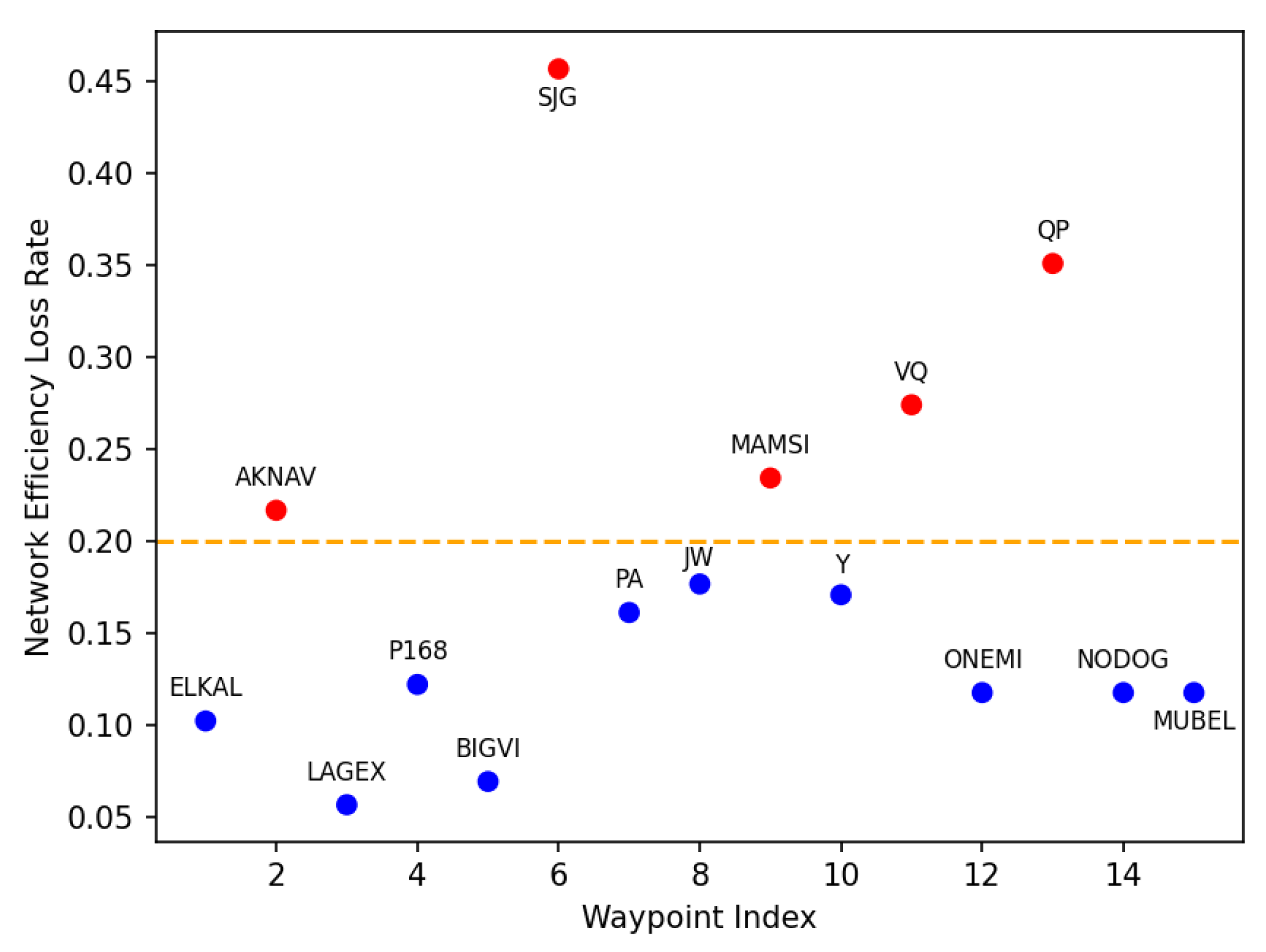
We calculate the network efficiency loss rates for each route point, as shown in Figure 8. The yellow dashed line in Figure 8 represents the boundary between the network efficiency loss rates of the first third and the last two-thirds of the nodes. It can be observed that route points SJG, QP, VQ, MAMSI, and AKNAV have relatively high network efficiency loss rates, indicating that these nodes have a significant impact on the reliability and performance of the system. They are thus considered critical nodes in the assessment of node importance. In actual operation, these route points serve as crossing points of multiple flight trajectories with a high node degree.

3. Methodology

3.1. Overall Framework of Prediction Process

Assuming a time interval of 15 min (i.e., two time steps), the node feature matrix of the route point network topology diagram G at a particular time step can be represented as follows:
X t = f 1 E 1 f M E M R M × P
where P represents the feature dimensions for each node (in this research P equals to 2), with f i and E i ( i = 1 , , M ) representing the traffic and network efficiency loss rate of the i-th node at this time step, respectively. The route point traffic prediction studied in this paper is a rolling prediction: using the spatiotemporal feature indicators of the route points from the preceding T continuous time intervals (specific indicators are detailed in Section 2.3), the route point traffic for the subsequent Q continuous time intervals is predicted.
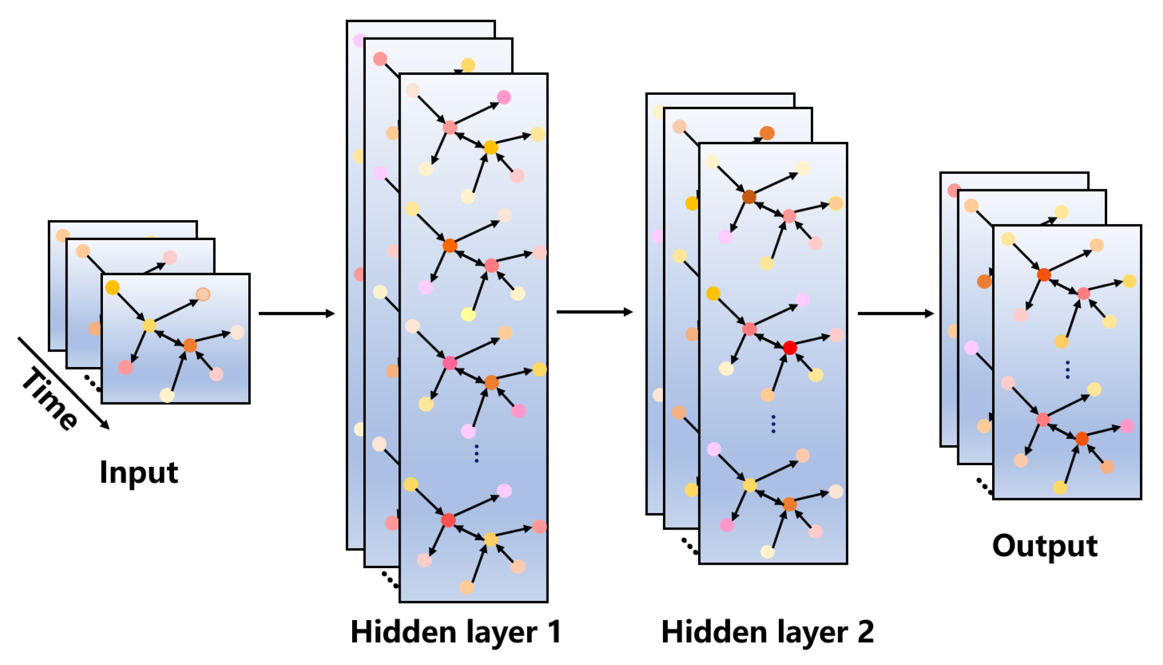
To extract the spatiotemporal features of route point traffic data more accurately, a neural network model based on graph convolutional network (GCN) and self-attention based long short-term memory network (SALSTM) is constructed, referred to as GC-SALSTM. This model is designed for short-term route point traffic prediction. The framework of the model is illustrated in Figure 9, comprising a GCN module and a LSTM module based on the self-attention mechanism. Firstly, the input consists of the route network topology diagram and the features of each route point over consecutive T time steps in the network. Then, the graph convolution module is employed to extract spatial features of the route point network. The LSTM module captures the temporal features of route point traffic, and the self-attention mechanism assigns different attention weights to each time step, further enhancing the prediction model accuracy. Lastly, a fully connected layer outputs predictions for the traffic at each route point over consecutive Q time steps.

3.2. Spatial Feature Extraction of Route Waypoint Traffic Based on GCN

A GCN is an approach for semi-supervised learning on graph-structured data and based on an efficient variant of convolutional neural networks operating directly on graphs. The input to the graph convolution module includes the route point network topology diagram G , the adjacency matrix A , and the feature matrix X t for each time step. Considering self-connection, the calculation formulas for the adjacency matrix A ˜ , the degree matrix D ˜ of route points, and the Laplacian matrix L are as follows:
A ˜ = A + I M
D ˜ = d i a g ( D ˜ 11 , D ˜ 22 , , D ˜ M M )
L = D ˜ 1 2 A ˜ D ˜ 1 2
where I M is the identity matrix, D ˜ i i = j A ˜ i j ; hence, the graph convolution formula is as follows:
H ( l + 1 ) = σ ( D ˜ 1 2 A ˜ D ˜ 1 2 H ( l ) W ( l ) )
where H ( l ) is the activation matrix for the layer l , with dimensions [ M , P ] , serving as the input to the layer l + 1 ; H ( 0 ) = X represents the initial input feature matrix of route points. W ( l ) is the trainable weight matrix used to modify the feature dimensions of route points, with dimensions [ P l , P l + 1 ] ; P l and P l + 1 are the feature dimensions of route points in the layer l and l + 1 , respectively. σ is the activation function. Additionally, in this study, the ReLU activation function [26] is employed. The graph convolution module is illustrated in Figure 10. After the graph convolution operation, spatial features of the route point network can be extracted.

3.3. Route Waypoint Traffic Prediction Based on Self-Attention LSTM

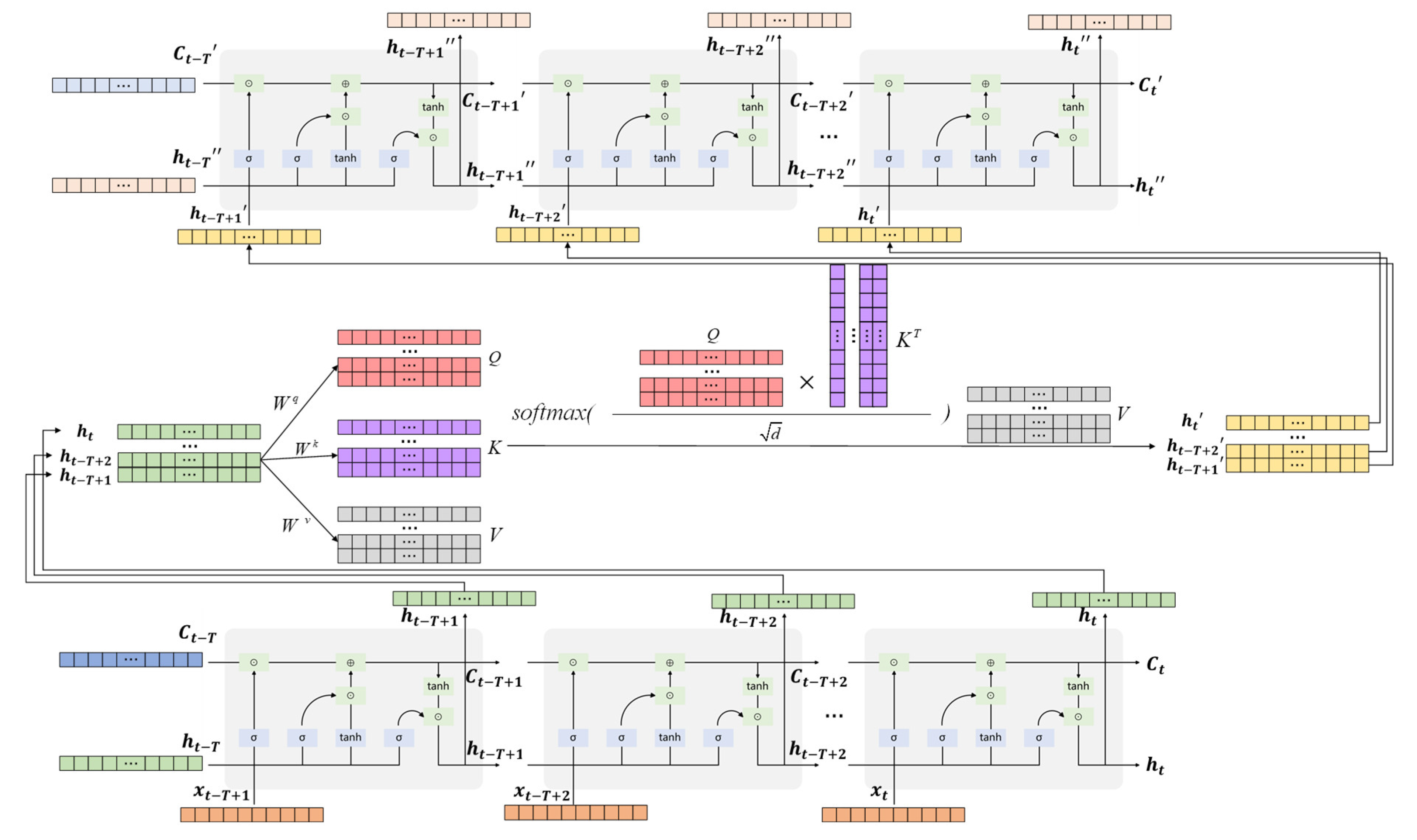
LSTM, a type of gated recurrent neural network (RNN), is effective in capturing temporal features of data and has been successfully applied to capture temporal features in traffic flow data [27,28,29,30,31]. In comparison to a traditional RNN, LSTM addresses the issues of vanishing and exploding gradients in longer time series prediction by introducing input gates, forget gates, and output gates to capture temporal dependencies over extended sequences effectively. The self-attention mechanism introduces attention at each time step of the input sequence to extract temporal correlation information from the input sequence. To enhance the accuracy of route point traffic prediction, this paper employs a route point traffic prediction method based on self-attention LSTM. Building upon the spatial features extracted via the GCN, the method focuses on extracting temporal features, as illustrated in the specific process outlined in Figure 11.
The module based on the self-attention LSTM consists of two LSTM layers and one self-attention layer. The spatial features x t at time step t , extracted using the GCN module, serve as the input to the LSTM module. Passing through the forget gate, input gate, update, and output gate, it outputs the hidden state h t and LSTM cell state C t . Subsequently, utilizing the self-attention mechanism, the attention size (i.e., the weight) between these T time steps is calculated. Based on these weights, a weighted average of the hidden states at these T time steps is obtained. This weighted hidden state is then used as the input to the next layer of LSTM for further temporal feature extraction. The formula for calculating the LSTM unit is as follows:
f t = σ ( W f [ h t 1 , x t ] + b f )
σ ( x ) = 1 1 + e x
i t = σ ( W i [ h t 1 , x t ] + b i )
C ˜ t = tanh ( W C [ h t 1 , x t ] + b C )
tanh ( x ) = e x e x e x + e x
C t = f t C t 1 + i t C ˜ t
o t = σ ( W o [ h t 1 , x t ] + b o )
h t = o t tanh ( C t )
where Equations (9) and (10) represent the forget gate of the LSTM unit, with f t representing the output of the forget gate, x t representing the input to the current state (i.e., the output of the GCN module at time t ), h t 1 representing the output of the previous hidden state, W f being the weight matrix, b f being the bias term, and σ being the sigmoid activation function. Equations (11)–(13) represent the input gate of the LSTM unit, where W i and W C are the weight matrices, b i and b C are the bias terms, and tanh is the activation function. Equation (14) is used to update the LSTM cell state, where C t 1 is the LSTM cell state from the previous time step, C t is the updated LSTM cell state at the current time step, and represents the Hadamard product. Equations (15) and (16) represent the output gate, where W o is the weight matrix and b o is the bias term.
The formula for calculating the self-attention mechanism is as follows:
h r W q = q r
h r W k = k r
h r W v = v r
a t , r = q t k r T d
a t , r = exp ( a t , r ) r exp ( a t , r )
h t = r a t , r v r
In Equations (17)–(19), h r represents the hidden state of the input time step r ( r = t T + 1 , t T + 2 , , t ) output from the LSTM module; W q , W k and W v are weight matrices. In Equations (20) and (21), d represents the variance of the matrix elements of Q × K T ; matrixes Q and K are defined as Q = ( q t T + 1 , , q t ) T and K = ( k t T + 1 , , k t ) T , respectively. a t , r denotes the attention weights from time step r to time step t . In Equation (22), h t represents the feature vector after attention weighting at time step t .
The weighted features h t from each time step are used as the input to the next layer of the LSTM network to further extract temporal features. The hidden state output from this LSTM layer is then fed into a fully connected layer, ultimately yielding the route point traffic predictions for the next consecutive Q time steps.

3.4. Definition of Loss Function

The objective of the GC-SALSTM model is to minimize the error between the predicted and actual route point traffic values. Mean square error (MSE), representing the Euclidean distance between predicted values and actual values, is employed as the model’s loss function and calculated as follows:
L o s s = 1 M n p = 1 M q = 1 n ( y ^ p , q y p , q ) 2
where M is the number of route points, n is the number of time steps, y ^ p , q is the predicted traffic value for route point p at time step q , and y p , q is the actual traffic value for route point p at time step q .

4. Experimental Analysis and Validation

4.1. Data

Air traffic and airspace data from 1 to 31 March 2019 in the Central and Southern Control Area were utilized. Traffic flow and network efficiency loss rate of 15 route points in sector 22 served as input features for the GC-SALSTM model. Experiments were conducted to validate the proposed prediction method’s effectiveness in the established environment.

4.2. Experimental Setup

The computer software and hardware configuration used for the calculations had the following specifications: operating system-Windows 11 (64-bit); processor-Intel(R) Core(TM) i7-1165G7 @ 2.80 GHz; CPU frequency-2.80 GHz; RAM-16.0 GB; programming language-Python 3.10.5; deep learning framework-TensorFlow 2.12.0.
To ensure the stability of the training process, data between 2:00 A.M. and 6:00 A.M. each day were excluded from the calculations of traffic and network efficiency loss rates. RMSProp optimizer is utilized. The specific model parameters are shown in Table 1. The division of the training set, validation set, and test set was performed using a time-series splitting method. This involved allocating the dataset into training, validation, and test sets based on the chronological order of time, following a specified ratio.
The model’s predictive performance was assessed using two metrics: mean absolute error (MAE) and RMSE.

4.3. Experiments and Analysis

4.3.1. Comparative Experiments on the Impact of Model Parameters on Prediction Performance

  • Comparison experiments for different numbers of GCN layers and dimensions
The number of convolutional layers in graph convolution and the different dimensions of each layer will affect the spatial feature extraction of the graph and the predictive performance of the model. Experiments were conducted to select parameters. The impact of different hidden layer dimensions under one layer of graph convolution and two layers of graph convolution on the model’s prediction results was tested, and the specific results are shown in Table 2.
From Table 2, it can be observed that when there is only one convolutional layer and the dimension is set to 32 (both MAE and RMSE are minimized), indicating the optimal predictive performance of the GC-SALSTM model. This is because, with a smaller dimension, there is less spatial feature extraction, resulting in poorer model prediction performance. On the other hand, with a larger dimension, although more spatial features can be extracted, it also introduces more parameters, leading to increased training time and a higher risk of overfitting, making it difficult to achieve the best predictive results.
Adding one more convolutional layer, when the dimension of the first convolutional layer is set to 32 and the second layer is set to 8, yields better prediction results. However, compared to having only one convolutional layer (with a dimension of 32), the prediction results are worse, with an increase of 12.18% in the RMSE. This suggests that, for the data used in this study, too many convolutional layers may not be suitable. A single convolutional layer can achieve good prediction results, and having too many layers may increase the risk of overfitting, thereby reducing the model’s predictive performance, which requires further research.
2.
Comparison experiments for different numbers of LSTM hidden neurons
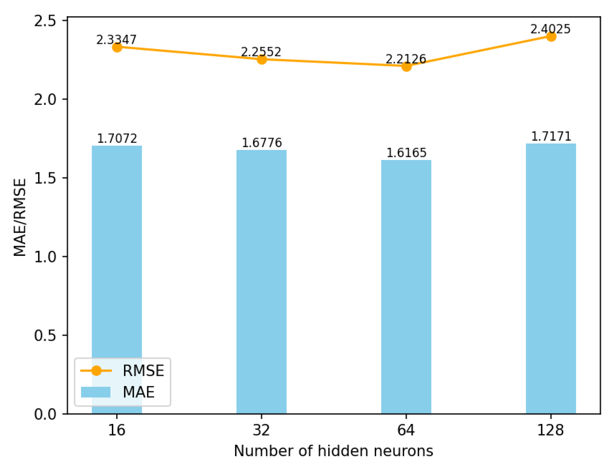
The number of LSTM hidden neurons affects the extent to which historical information is memorized, significantly impacting the model’s predictive results. To select a suitable number of LSTM hidden neurons, experiments were conducted with different numbers of hidden neurons (16, 32, 64, 128) for comparison. The results of the model’s MAE and RMSE are shown in Figure 12.
From Figure 12, it can be observed that the model achieves the best predictive results when the number of LSTM hidden neurons is set to 64. When the number of hidden neurons is less than 64 or greater than 64, the performance deteriorates. This indicates that with fewer neurons, the model’s ability to memorize historical information is poorer. On the other hand, with more neurons, the increased parameters lead to longer computation times and a higher risk of overfitting, resulting in reduced prediction accuracy.
3.
Comparison experiments for learning rate, training epochs, and batch size
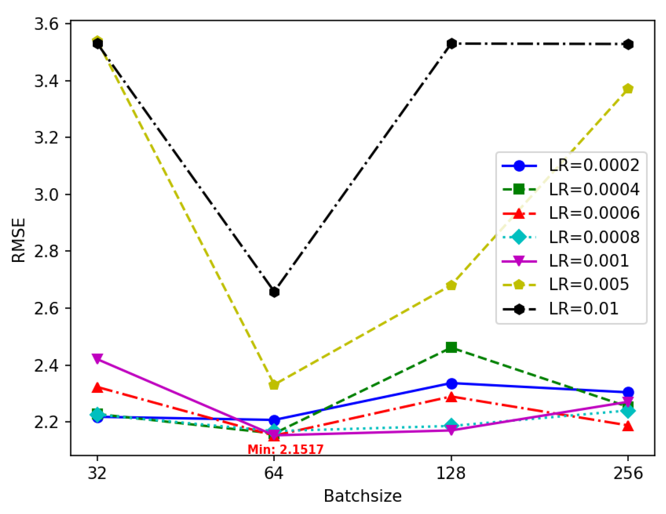
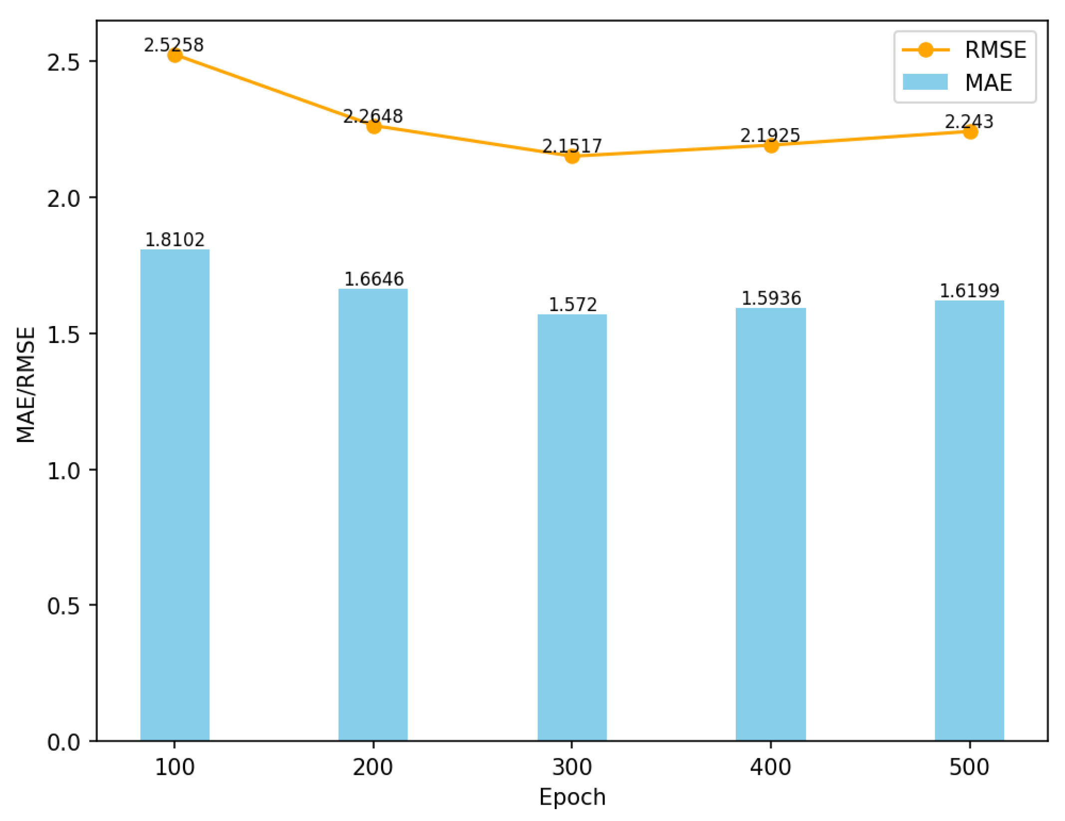
A learning rate that is too small may result in slow model convergence, while a learning rate that is too large may cause the model to oscillate near the minimum or even fail to converge. When the learning rate is small, more training epochs are needed to converge to the optimal result. However, excessively large training epochs may lead to overfitting, reducing prediction accuracy. A smaller batch size reduces the risk of overfitting, enhances generalization, but may result in lower prediction accuracy. Conversely, a larger batch size increases training time and the risk of overfitting, leading to suboptimal results on the test set. Therefore, careful selection of learning rate, training epochs, and batch size is crucial to further improve the model’s prediction accuracy.
Figure 13 shows the comparative experimental results for different learning rates and batch sizes. It can be observed that the model achieves the best prediction performance when the learning rate is 0.0006 and the batch size is 64.
Figure 14 illustrates the MAE and RMSE of the model’s predicted values for different numbers of training epochs (100, 200, 300, 400, 500). It can be observed that the prediction accuracy of the model decreases when the number of training epochs is too low or too high.
In summary, selecting appropriate learning rates, batch sizes, and training epochs plays a significant role in enhancing the predictive accuracy of the model.
4.
Experiment on input sequence length comparison
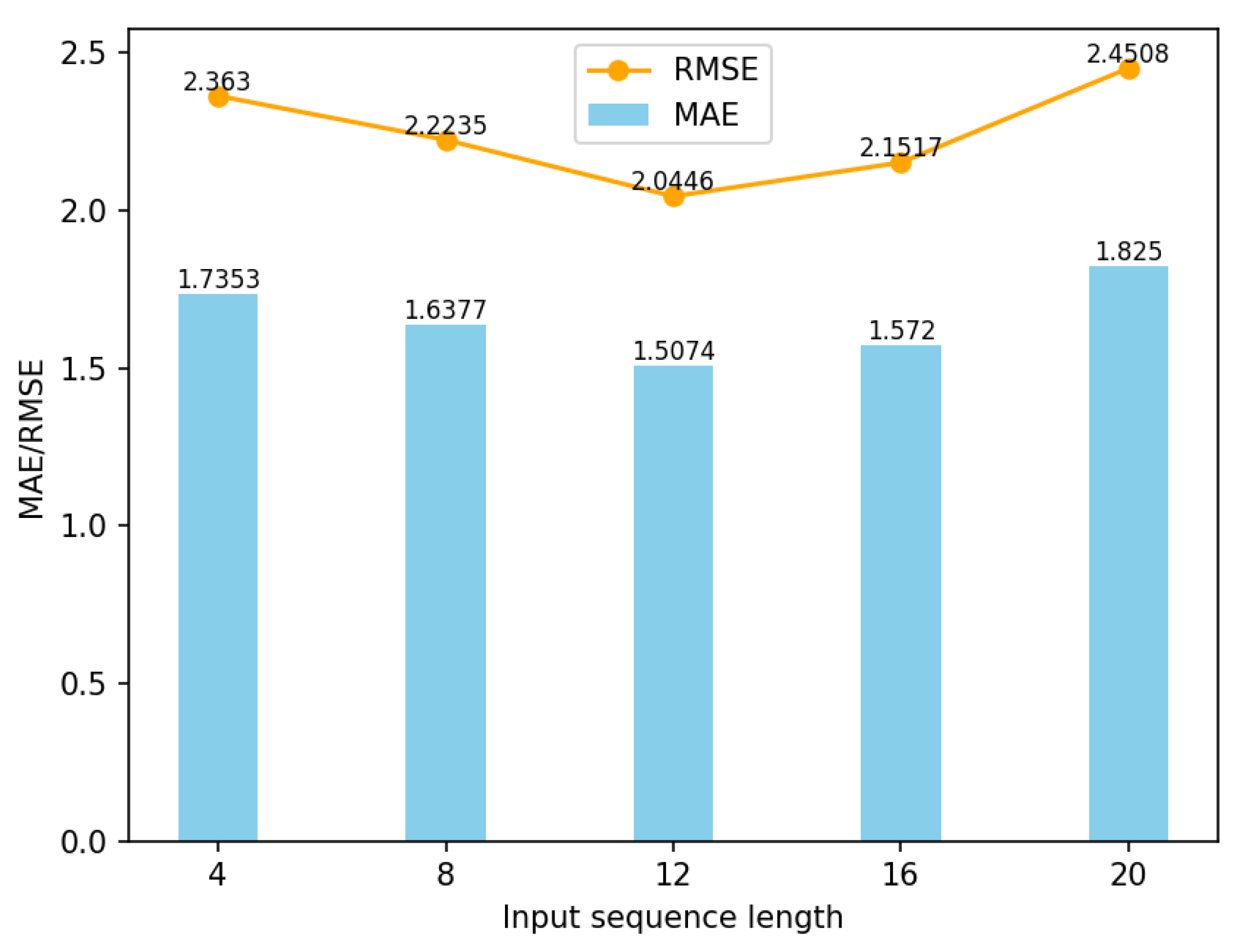
The output sequence length of the model in this paper is 4, predicting the future one-hour route point traffic flow. By testing different input sequence lengths of the model (4, 8, 12, 16, 20), it allows us to compare the prediction results to find the optimal input sequence length.
As shown in Figure 15, when the input sequence length is 12, i.e., predicting future one-hour traffic based on the past three hours of data, the model achieves the best prediction performance. With a shorter input sequence length, the prediction results are more influenced by individual data, leading to larger fluctuations and higher errors. On the other hand, with a longer input sequence length, the prediction results tend to be more averaged, making it difficult to capture fluctuations, resulting in larger errors.

4.3.2. Comparative Experiments on the Impact of Input Indicators on Prediction Performance

The input features of this model include the traffic of each waypoint and the network efficiency loss rate of waypoints. To validate the effectiveness of the network efficiency loss rate indicator, we compare the model’s prediction results when considering only traffic as input features versus when considering both traffic and network efficiency loss rate. We calculate the percentage change in RMSE after adding the network efficiency loss rate indicator.
The experimental results indicate that when adding the network efficiency loss rate indicator, the RMSE of the prediction results (2.0446) decreases by 17.42% compared to the RMSE of the predictions without this indicator (2.4760), showing a significant improvement.
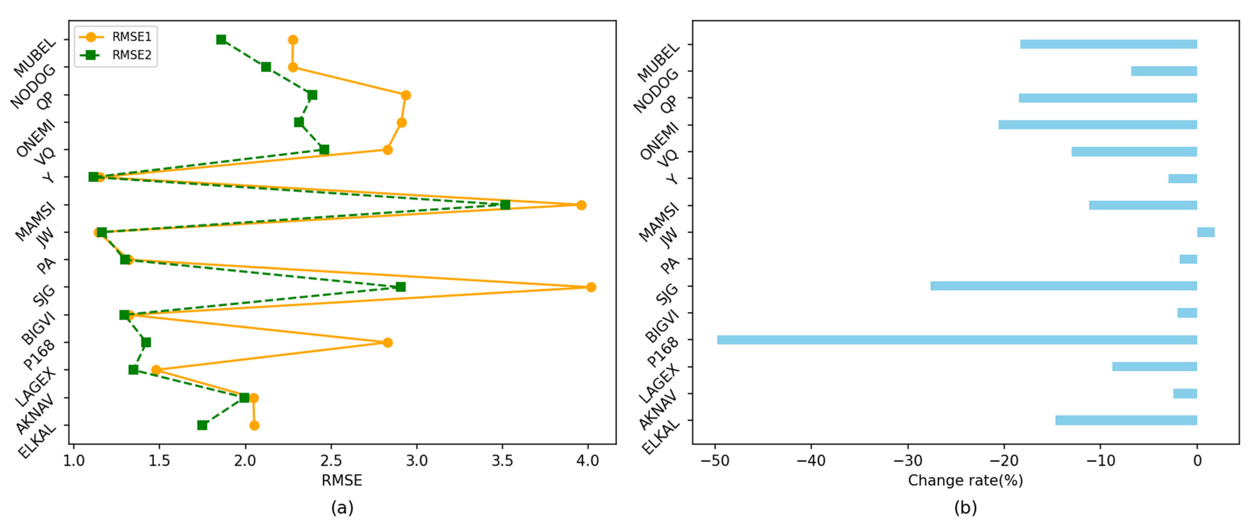
Figure 16a presents the RMSE of the model predictions at each waypoint when considering only the input parameter of flow and when considering two input parameters, namely the flow and network efficiency loss rate. Figure 16b illustrates the rate of change in the RMSE at each waypoint. In Figure 16a, RMSE1 refers to the prediction error of the model when the input metric is only the flow rate, while RMSE2 refers to the prediction error of the model when the input metrics are both the flow rate and network efficiency loss rate. It can be observed that after adding the network efficiency loss rate indicator, the RMSE of 14 route points decreases to varying degrees. Only one route point (JW) shows an increase of 1.83%, which is within an acceptable range. It is evident that adding the route point network efficiency loss rate indicator considers both the connectivity and distance factors, incorporating additional spatial correlation information extracted from the route point network, thereby enhancing the model’s prediction accuracy.
The impact of adding the network efficiency loss rate indicator on flow prediction accuracy of different route points was analyzed. The RMSE values for 8 route points decrease by more than 10%, including P168 (49.76%), SJG (27.66%), ONEMI (20.56%), QP (18.49%), MUBEL (18.30%), ELKAL (14.71%), VQ (13.02%), and MAMSI (11.20%). Among them, 5 route points have monthly traffic exceeding 10,000 flights, namely ONEMI (15,599 flights), SJG (18,193 flights), MAMSI (28,373 flights), VQ (15,757 flights), and QP (15,461 flights). There are four route points with a network efficiency loss rate exceeding 0.2, including SJG, MAMSI, VQ, and QP. If using monthly traffic exceeding ten thousand flights and a network efficiency loss rate exceeding 0.2 as criteria to identify key route points, then the key route points under this standard are SJG, MAMSI, VQ, and QP. These critical route points are the ones with a significant decrease in RMSE values after adding the network efficiency loss rate indicator. This indicates that the addition of the network efficiency loss rate indicator significantly enhances the prediction accuracy of the model, especially for critical route points. This has important implications for implementing real-time traffic management, thus optimizing slot and route resource allocation based on critical route points in air traffic. For instance, this provides more accurate traffic forecast values for resource allocation issues in flow constrained areas, etc.
Figure 17 displays the predicted traffic results for each route point throughout the day after adding the network efficiency loss rate indicator. From Figure 17, it can be observed that the MAMSI route point has significant traffic volume, with a peak prediction of 17 flights per 15 min. The VQ, ONEMI, QP, and SJG route points also have substantial traffic, with peak predictions of 9, 9, 9 and 10 flights per 15 min, respectively.

4.3.3. Comparative Experiments on Prediction Model Performance

When selecting the HA, ARIMA, SVR, LSTM, and GCN-LSTM models, a comparison of predictive performance was conducted against the GC-SALSTM model proposed in this study. The comparative results are shown in Table 3.
From Table 3, it can be observed that the GC-SALSTM model’s MAE and RMSE are reduced compared to the comparative models. Compared to the HA, ARIMA, SVR, LSTM, and GCN-LSTM models, the RMSE is reduced by 11.78%, 5.55%, 0.29%, 2.53%, and 1.09%, respectively. The MAE metric also shows a varying degree of improvement compared to the comparative models. The HA and ARIMA models, considering only temporal features and affected by the volatility of the data, exhibit relatively poor predictive performance. The SVR and LSTM models focus solely on temporal features without considering spatial features. Both the GCN-LSTM and the proposed model account for spatiotemporal correlation in traffic flow. The proposed model incorporates a self-attention mechanism, assigning different attention to different time steps, providing better modeling and prediction of spatiotemporal dependencies.
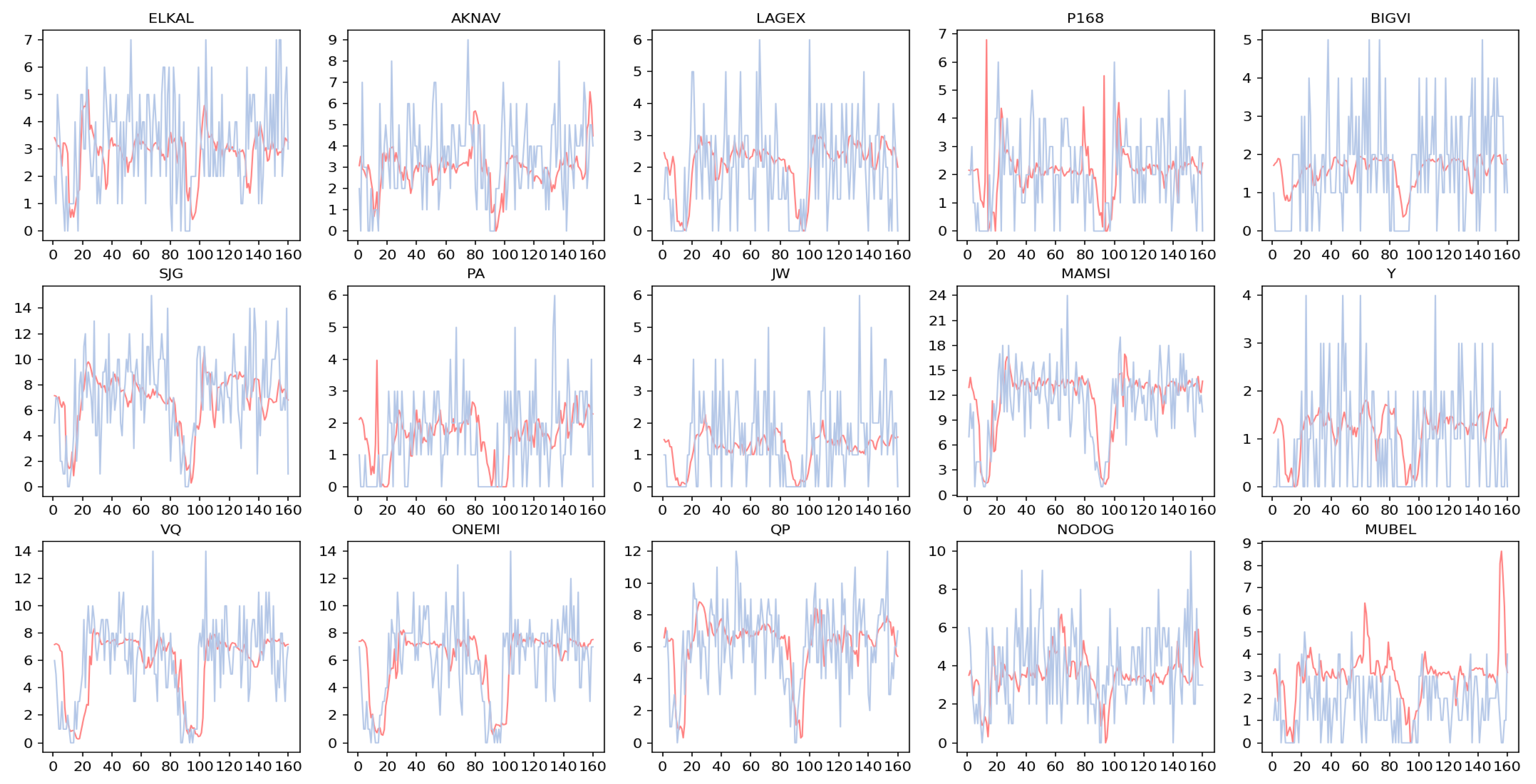
Figure 18 illustrates the comparison between the predicted traffic values using the GC-SALSTM model for 15 waypoints and the actual values, where the red line represents the predicted values, the blue line represents the actual values, the vertical axis denotes traffic flow, and the horizontal axis denotes the time steps. From the graph, it can be observed that the proposed model effectively captures the fluctuation trends in the traffic flow of the waypoints.

5. Conclusions and Further Discussion

In this paper, a neural network model combining graph convolution and self-attention long short-term memory was constructed, considering the spatial features of waypoint networks and the spatiotemporal characteristics of waypoint traffic. This model achieves the prediction of waypoint traffic for the next hour. The advantages of the model in this article are as follows. In addition to utilizing traffic flow data containing historical patterns, the input features of the model have been enhanced by incorporating the waypoint network efficiency loss rate indicator, further improving the prediction accuracy of traffic flow for critical waypoints.
By analyzing and validating the ZGGGAR22 sector waypoints in the Central and Southern region in China, the results indicate that the predictive accuracy of the GC-SALSTM model is improved compared to typical forecasting models such as the HA, ARIMA, SVR, LSTM, and GCN-LSTM models. With the addition of the waypoint network efficiency loss rate as an input feature, the RMSE for 8 waypoints has decreased by more than 10%. This provides an effective method for identifying and predicting congestion points and congested periods in the waypoint network, offering more accurate information for real-time air traffic management and resource allocation in air traffic control.
The drawbacks of the model in this article include a limited number of input indicators and a lack of consideration for external factors, such as weather conditions. Future research directions: This paper focuses on the spatiotemporal correlation features of waypoint traffic flow within the sector for waypoint flow prediction. The research scope can be further expanded by constructing a wide-area waypoint-connected traffic network topology, incorporating external factors such as weather, and effectively utilizing and integrating multi-source data into the prediction method. Considering the practical application needs of traffic flow prediction, the goal is to enhance and improve prediction effectiveness with a focus on predictive applications. In addition to traffic flow, various prediction contents, such as traffic operation speed, traffic complexity, delays, etc., can also be considered for analysis and prediction.

Author Contributions

Conceptualization, W.T. and Y.Z. (Yining Zhang); methodology, Y.Z. (Yining Zhang); software, Y.Z. (Yining Zhang) and H.C.; validation, W.T., Y.Z. (Yining Zhang) and Y.Z. (Ying Zhang); formal analysis, W.T. and Y.Z. (Yining Zhang); investigation, W.L.; resources, W.T.; data curation, W.T., Y.Z. (Yining Zhang) and Y.Z. (Ying Zhang); writing—original draft preparation, Y.Z. (Yining Zhang); writing—review and editing, W.T., Y.Z. (Ying Zhang) and H.C.; visualization, W.T. and Y.Z. (Yining Zhang); supervision, W.L.; project administration, W.T., Y.Z. (Ying Zhang) and H.C.; funding acquisition, W.T. and Y.Z. (Yining Zhang). All authors have read and agreed to the published version of the manuscript.

Funding

This research was funded by the National Key R&D Program of China, grant number 2022YFB2602403; the National Natural Science Foundation of China, grant number 71971112; the School Innovation Plan Project of Nanjing University of Aeronautics and Astronautics, grant number xcxjh20230718; and the Jiangsu Provincial Natural Science Foundation General Project, grant number BK20231447.

Data Availability Statement

Data are contained within the article.

Acknowledgments

We thank the State Key Laboratory of Air Traffic Management System for supporting this research.

Conflicts of Interest

The authors declare no conflicts of interest.

References

  1. Yang, L.; Yin, S.W.; Hu, M.H. Network flow dynamics modeling and analysis of arrival traffic in terminal airspace. IEEE Access 2019, 7, 73993–74016. [Google Scholar] [CrossRef]
  2. Pawelek, A.; Lichota, P. Arriving air traffic separations generalized model identification. Bull. Pol. Acad. Sci. Tech. Sci. 2022, 70, e140556. [Google Scholar] [CrossRef]
  3. Xu, Y.; Zhang, H.H.; Liao, Z.H.; Yang, L. A dynamic air traffic model for analyzing relationship patterns of traffic flow parameters in terminal airspace. Aerosp. Sci. Technol. 2016, 55, 10–23. [Google Scholar] [CrossRef]
  4. Yao, J.F.; He, R.; Shi, T.T.; Wang, P.; Zhao, X.M. Review on machine learning-based traffic flow prediction methods. J. Traffic Transp. Eng. 2023, 23, 44–67. [Google Scholar] [CrossRef]
  5. An, J.Y.; Fu, L.; Hu, M.; Chen, W.H.; Zhan, J.W. A novel fuzzy-based convolutional neural network method to traffic flow prediction with uncertain traffic accident information. IEEE Access 2019, 7, 20708–20722. [Google Scholar] [CrossRef]
  6. Cui, Z.Y.; Ke, R.M.; Pu, Z.Y.; Wang, Y.H. Stacked bidirectional and unidirectional LSTM recurrent neural network for forecasting network-wide traffic state with missing values. Transp. Res. Part C-Emerg. Technol. 2020, 118, 102674. [Google Scholar] [CrossRef]
  7. Zhao, L.; Song, Y.J.; Zhang, C.; Liu, Y.; Wang, P.; Lin, T.; Deng, M.; Li, H.F. T-GCN: A Temporal Graph Convolutional Network for Traffic Prediction. IEEE Trans. Intell. Transp. Syst. 2020, 21, 3848–3858. [Google Scholar] [CrossRef]
  8. Gu, Z.Y.; Chen, C.; Zheng, J.J.; Sun, D.H. Traffic Flow Prediction Based on STG-CRNN. Control Decis. 2023, 38, 3399–3408. [Google Scholar] [CrossRef]
  9. Chen, Z.J.; Lu, Z.; Chen, Q.S.; Zhong, H.L.; Zhang, Y.S.; Xue, J.; Wu, C.Z. A spatial-temporal short-term traffic flow prediction model based on dynamical-learning graph convolution mechanism. Inf. Sci. 2022, 611, 522–539. [Google Scholar] [CrossRef]
  10. Zhang, Y.J. Research on Prediction Method of Ride-Hailing Demand Based on Spatio-Temporal Graph Neural Network. Master’s Thesis, Beijing Jiaotong University, Beijing, China, 2022. [Google Scholar] [CrossRef]
  11. Cui, W.Y.; Gu, Y.L.; Zhao, S.L.; Rui, X.P. A method of Predicting Short-term Traffic Flows Based on a DGC-GRU Model. J. Transp. Inf. Saf. 2023, 41, 121–128. [Google Scholar] [CrossRef]
  12. He, W.W.; Pei, B.Y.; Li, Y.T.; Liu, X.Y.; Xu, S.B. Traffic Flow Forecasting Based on Bi-directional Adaptive Gating Graph Convolutional Networks. J. Transp. Syst. Eng. Inf. Technol. 2023, 23, 187–197. [Google Scholar] [CrossRef]
  13. Lin, Y.; Zhang, J.W.; Liu, H. Deep learning based short-term air traffic flow prediction considering temporal-spatial correlation. Aerosp. Sci. Technol. 2019, 93, 105113. [Google Scholar] [CrossRef]
  14. Yang, Z.; Tang, R.; Zeng, W.L.; Lu, J.H.; Zhang, Z.J. Short-term prediction of airway congestion index using machine learning methods. Transp. Res. Part C-Emerg. Technol. 2021, 125, 103040. [Google Scholar] [CrossRef]
  15. Bao, J.; Yang, Z.; Zeng, W.L. Graph to sequence learning with attention mechanism for network-wide multi-step-ahead flight delay prediction. Transp. Res. Part C-Emerg. Technol. 2021, 130, 103323. [Google Scholar] [CrossRef]
  16. Liu, X.L.; Guo, M.J.; Li, Z. Flight delay prediction based on attention-based adaptive graph convolution-Gated Recurrent Unit. J. Beijing Univ. Aeronaut. Astronaut. 2023, 48, 1–16. [Google Scholar] [CrossRef]
  17. Wang, L.L.; Zhao, Y.F. A Method for Predicting Air Traffic Flow Based on a Combined GA, RBF, and Improved Cao Method. J. Transp. Inf. Saf. 2023, 41, 115–123. [Google Scholar] [CrossRef]
  18. Yan, Z.; Yang, H.Y.; Li, F.; Lin, Y. A Deep Learning Approach for Short-Term Airport Traffic Flow Prediction. Aerospace 2021, 9, 11. [Google Scholar] [CrossRef]
  19. Zhong, J.; Zhang, Y.J.; Wang, J.Y.; Luo, C.; Miao, Q. Unmanned Aerial Vehicle Flight Data Anomaly Detection and Recovery Prediction Based on Spatio-Temporal Correlation. IEEE Trans. Reliab. 2021, 71, 457–468. [Google Scholar] [CrossRef]
  20. Kamo, S.; Rosenow, J.; Fricke, H.; Soler, M. Fundamental Framework to Plan 4D Robust Descent Trajectories for Uncertainties in Weather Prediction. Aerospace 2022, 9, 109. [Google Scholar] [CrossRef]
  21. Rodríguez-Sanz, Á.; Comendador, F.G.; Valdés, R.A.; Pérez-Castán, J.; Montes, R.B.; Serrano, S.C. Assessment of airport arrival congestion and delay: Prediction and reliability. Transp. Res. Part C Emerg. Technol. 2019, 98, 255–283. [Google Scholar] [CrossRef]
  22. Zhao, Z.; Yuan, J.L.; Chen, L.H. Air Traffic Flow Management Delay Prediction Based on Feature Extraction and an Optimization Algorithm. Aerospace 2024, 11, 168. [Google Scholar] [CrossRef]
  23. Chen, D.; Hu, M.H.; Zhang, H.H.; Yin, J.N.; Han, K. A network based dynamic air traffic flow model for en route airspace system traffic flow optimization. Transp. Res. Part E Logist. Transp. Rev. 2017, 106, 1–19. [Google Scholar] [CrossRef]
  24. Li, L.; Liang, Y.; Lin, N.; Yan, J.; Meng, H.; Liu, Y.Q. Data cleaning method considering temporal and spatial correlation for measured wind speed of wind turbines. Acta Energiae Solaris Sin. 2023. [CrossRef]
  25. Tian, W.; Fang, Q.; Zhou, X.F.; Song, J.J. Research on Identification Method of Key Nodes in En-route Network. J. Southwest Jiaotong Univ. 2022, 1–10. Available online: http://kns.cnki.net/kcms/detail/51.1277.U.20221124.0859.002.html (accessed on 25 November 2022).
  26. Shi, S.H.; Chu, X.W. Speeding up convolutional neural networks by exploiting the sparsity of rectifier units. arXiv 2017, arXiv:1704.07724. [Google Scholar] [CrossRef]
  27. Xiao, Y.L.; Yin, Y. Hybrid LSTM Neural Network for Short-Term Traffic Flow Prediction. Information 2019, 10, 105. [Google Scholar] [CrossRef]
  28. Afrin, T.; Yodo, N. A Long Short-Term Memory-based correlated traffic data prediction framework. Knowl.-Based Syst. 2022, 237, 107755. [Google Scholar] [CrossRef]
  29. Mou, L.T.; Zhao, P.F.; Xie, H.T.; Chen, Y.Y. A Long Short-Term Memory Neural Network Enhanced by Temporal Information for Traffic Flow Prediction. IEEE Access 2019, 7, 98053–98060. [Google Scholar] [CrossRef]
  30. Ma, C.X.; Dai, G.W.; Zhou, J.B. Short-Term Traffic Flow Prediction for Urban Road Sections Based on Time Series Analysis and LSTM_BILSTM Method. IEEE Trans. Intell. Transp. Syst. 2022, 23, 5615–5624. [Google Scholar] [CrossRef]
  31. Fang, W.W.; Zhuo, W.H.; Song, Y.Y.; Yan, J.W.; Zhuo, T.; Qin, J. Dfree-LSTM: An error distribution free deep learning for short-term traffic flow forecasting. Neurocomputing 2023, 526, 180–190. [Google Scholar] [CrossRef]
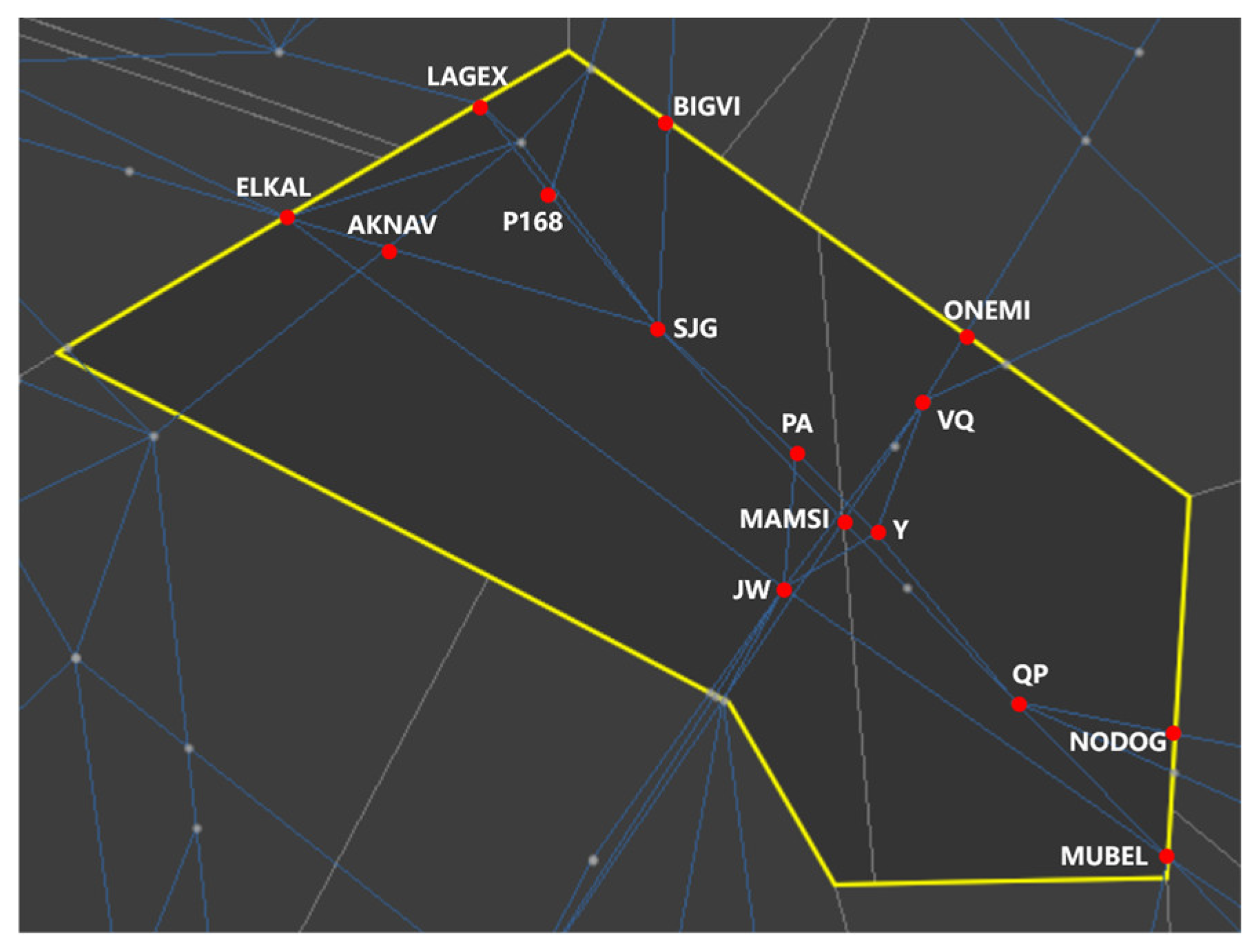
Figure 1. Diagram of typical busy sector ZGGGAR22 with route waypoints.
Aerospace 11 00248 g001
Figure 2. Waypoint network topology diagram.
Aerospace 11 00248 g002
Figure 3. Full-day traffic distribution of key waypoints in the Greater Bay Area airport group.
Aerospace 11 00248 g003
Figure 4. Traffic distribution chart for waypoint MAMSI on consecutive Mondays over four weeks.
Aerospace 11 00248 g004
Figure 5. Pearson’s coefficient of the time series traffic flow at waypoint MAMSI for each time interval.
Aerospace 11 00248 g005
Figure 6. Traffic distribution chart for different waypoints on a specific day.
Aerospace 11 00248 g006
Figure 7. Pearson’s coefficients of the traffic time series for 15 waypoints.
Aerospace 11 00248 g007
Figure 8. Efficiency loss rate for each waypoint in the network.
Aerospace 11 00248 g008
Figure 9. Framework diagram of GC-SALSTM model’s composition.
Aerospace 11 00248 g009
Figure 10. Illustration of graph convolutional module.
Aerospace 11 00248 g010
Figure 11. Illustration of a self-attention LSTM module.
Aerospace 11 00248 g011
Figure 12. Experimental results on the comparison of the number of hidden neurons in LSTM.
Aerospace 11 00248 g012
Figure 13. Experimental results on the comparison of learning rates and batch data processing sizes.
Aerospace 11 00248 g013
Figure 14. Experimental results on the comparison of training epochs.
Aerospace 11 00248 g014
Figure 15. Experimental results on the comparison of input sequence lengths.
Aerospace 11 00248 g015
Figure 16. Experimental results on the comparison of input metrics: (a) RMSE for model predictions at waypoints with flow parameter alone and with flow & network efficiency loss rate parameters; (b) rate of change in the RMSE at each waypoint.
Aerospace 11 00248 g016
Figure 17. Predicted traffic volumes for each waypoint throughout the day in different time periods.
Aerospace 11 00248 g017
Figure 18. Comparison between predicted and actual traffic values for 15 waypoints.
Aerospace 11 00248 g018
Table 1. Model parameters.
ParameterValue
Training set ratio75%
Validation set ratio5%
Test set ratio20%
Number of graph convolution layer1
Dimension of graph convolution layer32
Number of hidden neurons64
Training epochs300
Batch size64
Learning rate0.0006
Input sequence length12
Prediction sequence length4
Table 2. Comparison of performance based on different graph convolutional layer numbers and dimensions.
The First Convolutional LayerThe Second Convolutional Layer
DimensionMAERMSEDimensionMAERMSE
161.71452.328481.79852.4538
161.79622.4818
321.61112.199481.77722.4672
161.89432.5784
322.01712.8346
641.61872.215181.88832.6100
161.82842.5696
321.79892.4462
641.81892.5872
1281.66612.291281.89312.5782
161.85982.6035
321.94792.7601
641.85282.4914
1281.80192.4952
Table 3. Prediction error results for each model.
ModelMAERMSE
HA1.69282.3176
ARIMA1.75562.1647
SVR1.53672.0506
LSTM1.53062.0977
GCN-LSTM1.53862.0672
GC-SALSTM1.50742.0446
Disclaimer/Publisher’s Note: The statements, opinions and data contained in all publications are solely those of the individual author(s) and contributor(s) and not of MDPI and/or the editor(s). MDPI and/or the editor(s) disclaim responsibility for any injury to people or property resulting from any ideas, methods, instructions or products referred to in the content.