Predicting Air Traffic Congestion under Uncertain Adverse Weather

Abstract

This paper presents an approach for integrating uncertainty information in air traffic flow management at the tactical phase. In particular, probabilistic methodologies to predict sector demand and sector congestion under adverse weather in a time horizon of 1.5 h are developed. Two sources of uncertainty are considered: the meteorological uncertainty inherent to the forecasting process and the uncertainty in the take-off time. An ensemble approach is adopted to characterize both uncertainty sources. The methodologies rely on a trajectory predictor able to generate an ensemble of 4D trajectories that provides a measure of the trajectory uncertainty, each trajectory avoiding the storm cells encountered along the way. The core of the approach is the statistical processing of the ensemble of trajectories to obtain probabilistic entry and occupancy counts of each sector and their congestion status when the counts are compared to weather-dependent capacity values. A new criterion to assess the risk of sector overload, which takes into account the uncertainty, is also defined. The results are presented for a historical situation over the Austrian airspace on a day with significant convection.

1. Introduction

Air Traffic Flow and Capacity Management (ATFCM) is one of the components of the European Air Traffic Management (ATM). Its aim is to manage the balance of demand and capacity by optimizing the use of available resources and coordinating adequate responses [1]. This function is vital under an ever-growing traffic demand, and particularly during disruptive events such as adverse weather, military exercises, higher-airspace/space operations, and periods of peak demand.

Among the most disruptive events for aviation, severe convective storms are especially challenging during summertime in Europe [2]. Formed by heavy and dense clouds of great height known as cumulonimbus clouds, which may cover hundreds of kilometers and last up to several hours [3], they represent a dynamic hazard for flights because of their associated damaging phenomena, e.g., turbulence, strong winds, icing, lightning, or hail. See, for example, a recent case over Italy [4].

In the event of a thunderstorm, ATFCM, as usual, considers all possible solutions through an iterative process, from the strategic planning to the execution of operations. The various ATFCM solutions depend on the severity of the capacity shortfall, and range from optimizing the use of the available capacity, e.g., change of sector configuration, to regulating the demand, e.g., slot allocation of flights. Ideally, the earlier actions can be taken, the easier it will be to minimize the impact on the network. However, this is not always possible because the evolution of thunderstorms is very difficult to predict, particularly in the long term (beyond 2 h). While some meteorological conditions required for thunderstorm formation can be forecasted in advance, the specific location, geometry, and timing of storm cells are much harder to anticipate. This fact typically leads to a reactionary response, applied when most flights are already airborne.

Deciding which solutions to implement and how to implement them is not straightforward as some aircraft may reroute their flight plans to avoid the regulations [5] and each ATFCM solution presents many parameters to configure [6]. Furthermore, flight deviations to avoid the storm cells have a negative effect on the workload of air traffic controllers because the traffic flow becomes irregular and not easy to anticipate, radio-communications are increased, and less airspace volume is available for conflict resolution, thereby reducing sectors’ capacity.

To support justified decisions in line with the principles of safety and efficiency, the information available to the Flow Management Position (FMP)—a role within the Air Navigation Service Providers of each State, typically located at the Area Control Centres (ACCs)—should be as useful as possible. To this end, the FMP has the Collaborative Interface for Flow Management Positions (CIFLO) application [7]. CIFLO provides real-time information from the network operations systems and displays data and graphical information via maps. Nowadays, the traffic is monitored by using hourly sector entries, although the utilization of sector occupancy is becoming more widespread [8]. The values of the predicted demand incorporate the best available information about each flight: real departure time, regulations, and any subsequent updates. Nonetheless, a low adherence to filed flight plans, along with a lack of coordination, has been shown to be a persistent issue [9], with only 50% of traffic actually flying through sectors at the planned times. Therefore, there is incentive, and also room, for improvement.

Moreover, meteorological information is poorly integrated into the decision-making process. FMPs and ACC Supervisors tasked with Configuration Management brief themselves of relevant meteorological conditions on various separate briefing systems not included in CIFLO, and they convert this information into impact on sector monitoring values (MVs)—the agreed number of flights accepted into a sector [7]—and integrate them manually into the current CIFLO. The risks here are many, from the FMP not understanding the potential negative impact and causing an overload/overdelivery on the sectors, to overregulating despite having a very low intensity weather.

In view of all the above, there is a need for improving the prediction of traffic demand, particularly in a scenario of weather uncertainty, and for developing a strategy that integrates meteorological forecasts into the decision-making process. This paper seeks to address such needs.

When forecasting traffic demand, the results obtained with a probabilistic approach have proven to be better than deterministic estimations according to past studies. In particular, an improvement of 15 to 20% is found in [10], where the probabilistic demand at an airport is calculated via Monte Carlo simulations. A similar finding is obtained for the en-route traffic in [11], now with respect to the deterministic prediction of the flight plans (FPLs) at three time horizons: 3 h before flight time, 1 h before flight time, and at the time of the last filed FPL.

The preferred approach for the probabilistic methodologies considers an ensemble of probable trajectories for each flight. This is the strategy followed in [12], presenting a vision of the integration of ensemble weather forecasts in ATM decision support tools, and is also chosen, for example, for the studies conducted within the framework of the Combining Probable Trajectories (COPTRA) project [13]. Here, the researchers assume the predominance of temporal uncertainty, and, without loss of generality, use a Gaussian distribution with a standard deviation of 14.4 min to model the sector entry and exit times of each flight.

With respect to the prediction of demand–capacity imbalances in a particular airspace, the efforts made in the past can be grouped into two different approaches: the separate prediction of traffic counts and capacity values and the subsequent comparison between them, or the direct prediction of the congestion status. The first approach is the one followed by the Network Manager, and the one proposed by [14] for a probabilistic methodology. The work [15] follows the second approach to directly predict the activation of Air Traffic Flow Management (ATFM) regulations by using machine learning and historical data.

The use of Machine Learning (ML) techniques for sector demand prediction has received growing attention in recent years. One example is [16], where the authors attempt to predict the occupancy in the Maastricht Upper Area Control Centre based, among others, on a set of weather-related features (number of air-blocks containing an overshoot of storm, a high, and a very high storm severity). Another example is [17]. Here, the focus is on general aviation. The paper describes an ML-based methodology to predict the traffic demand over the Nice Cote D’Azur Terminal Control sectors, with a time horizon of 4 h.

Our preliminary work on this problem [18,19,20,21], presented at various conferences, is described next. In [18], we present preliminary results on sector demand prediction considering wind uncertainty. This work is extended in [19] considering the presence of thunderstorms. In that study, we present an ensemble-based probabilistic methodology that predicts sector occupancies with a forecasting horizon of 15 min. Supported by two technical enablers, namely, a probabilistic weather forecast and a probabilistic trajectory predictor, the resulting ensemble accounts for the uncertainty in the location of the convective cells affecting the sector and its vicinity. The outcomes show that the sector demand subject to thunderstorm uncertainties can be accurately predicted in the very short term. However, these outcomes are limited by several assumptions made—some of them inherent to the input data: the shape of all the convective cells is elliptical; the only source of uncertainty in the flight deviations is the location of such ellipses; and the sector is considered two-dimensional. The third work [20] focuses on the description of an integrated trajectory predictor developed to analyze the problem for a look-ahead time of up to 8 h. Finally, the fourth work [21] focuses on how much airspace capacity can be affected by uncertain adverse weather, also within a look-ahead time of up to 8 h.

In this paper, we present the final results for sector demand and sector congestion prediction for a look-ahead time of 1.5 h, which lies within common practice for short-term forecasting (typically up to 2 h, e.g., [22,23]). We consider a refined methodology which includes multiple spatio-temporal uncertainty sources, more realistic storm contours, and the three-dimensionality of sectors. We follow a probabilistic approach, based on an ensemble of possible scenarios, where probabilistic traffic counts and probabilistic capacity thresholds are predicted, subject to the same weather forecasts, and then compared to obtain a prediction of congestion. In particular, we are interested in the en-route problem and consider two uncertainty sources: the meteorological uncertainty inherent to the forecasting process and the uncertainty in the take-off time.

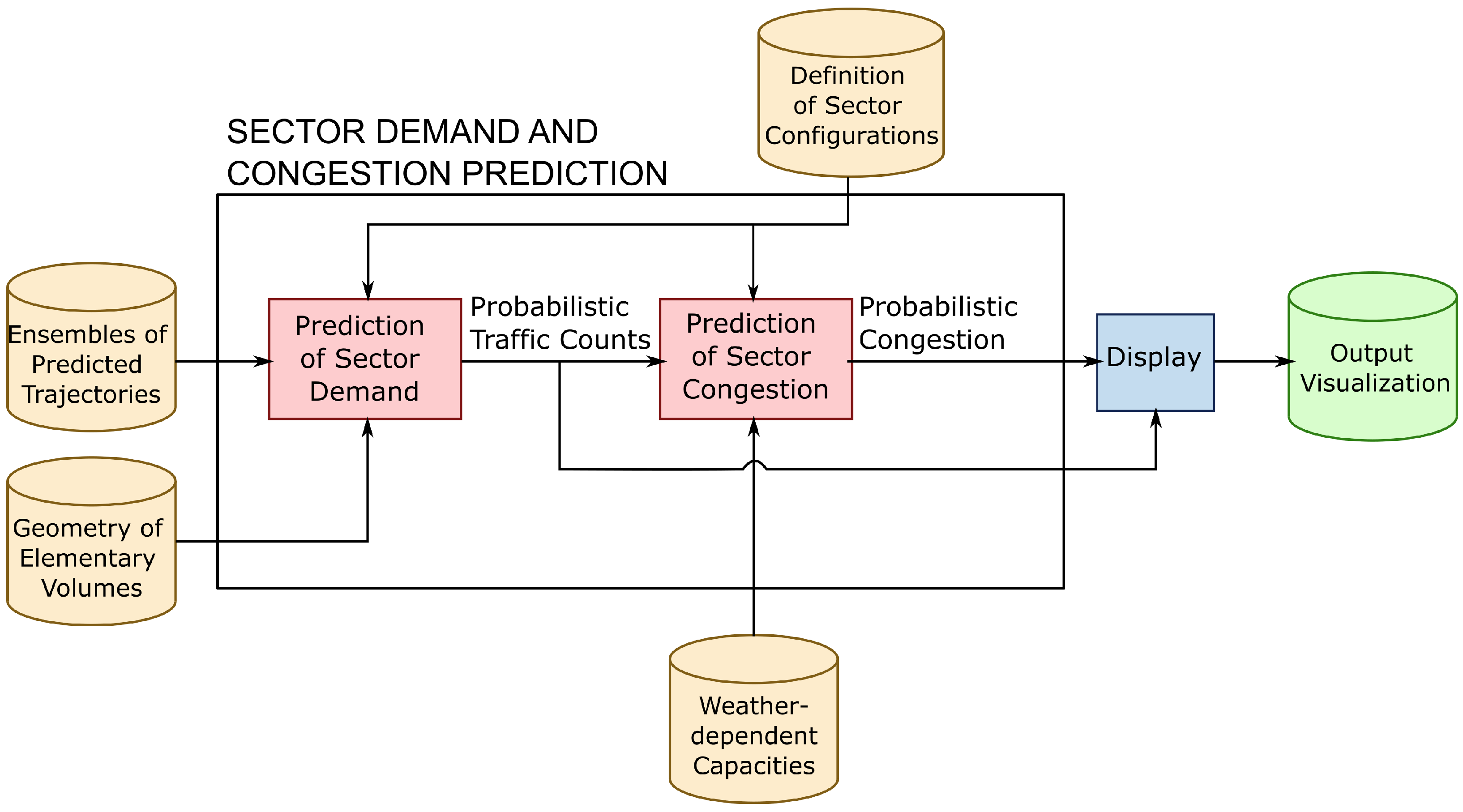
Our main contribution is the probabilistic methodologies to predict sector demand and sector congestion, including a new probabilistic criterion to assess the risk of sector overload. The sector demand is obtained in the form of probabilistic entry and occupancy counts (other authors suggest a different approach based on traffic flows, e.g., [24]). These are calculated by statistically processing the set of entry and occupancy counts associated with the ensembles of predicted trajectories. In turn, for the determination of these traffic counts, it is necessary to find the entry and exit times of each predicted trajectory in a given airspace scenario. To evaluate the sector congestion, the available capacity needs to be known. In this paper, the capacity reduction caused by adverse weather is taken as an input. The final objective is to use these predictions to evaluate the future congestion status of the sectors, similarly to how it is conducted in CIFLO, to determine whether or not applying an ATFCM measure is needed. A schematic diagram showing the required inputs is depicted in Figure 1.

This paper is structured as follows. First, the two uncertainty sources considered in this work are described in Section 2. Second, the methodologies designed to calculate probabilistic sector demand and congestion are presented in Section 3 and Section 4. Then, the previous methodologies are applied to a case study defined in Section 5. The results of the case study are shown and discussed in Section 6. Finally, Section 7 provides a summary with the main contributions of this work and a proposal for future research.

2. Uncertainty Characterization

In this work, we assume that a correct probabilistic characterization of entry and occupancy counts in a scenario of adverse weather requires the consideration of spatiotemporal uncertainties. In particular, we incorporate the uncertainty in the weather forecast, which accounts for the possible locations, extensions, and durations of storm cells, and the uncertainty in the take-off time. The latter accounts not only for possible regulations due to the existing/forecasted weather conditions, but also for the stochastic behavior of flight departures, which, to a similar degree, determine the moment when weather encounters occur, hence pilots and traffic controllers’ responses. An additional uncertainty source could be the one in the pilots’ avoidance strategy. However, the influence of non-weather related factors on pilots’ maneuvers in a scenario of meteorological hazard is not clear according to the relevant literature [25,26,27,28,29], and the only agreement seems to be that operational factors—e.g., type and density of traffic, available airspace capacity, leader/follower roles and flight delays—are less important than weather-related factors. Therefore, we decided not to include it in our study.

In this section, the considered sources of uncertainty that affect the generation of the probabilistic trajectories are analyzed. Modeling in both cases is performed by means of an ensemble-based approach. Thus, once the uncertainties are characterized, the input will be an ensemble of $N_w$ weather scenarios—hereafter identified as members—and an ensemble of $N_d$ take-off time members.

2.1. Weather Ensemble Members

Considering the time horizon of 90 min and the presence of thunderstorms, weather forecast uncertainty is given by an ensemble nowcast, composed of a number of statistically independent nowcasts –identified by the value of the index k$(k=1,\dots ,N_w)$—constituting a representative sample of the possible weather realizations, which are the result of extrapolating the latest observed state of the atmosphere.

In this work, the nowcast used is based on the Short Term Ensemble Prediction System (STEPS) methodology [30], based on radar and satellite observations, composed of 15 members, and successfully assessed near our area of interest [31]. The information contained in the nowcasts include the position, extensions, and strengths of the existing convective cells as well as the top height of their clouds (CTH). The identification of the storm cells is performed through (1) the conversion of the convective rain rate into radar reflectivity using the Marshall–Palmer relationship, and (2) the consideration of a reflectivity threshold of 38 dBz [32]. As a conservative approach, a single and deterministic CTH value was considered for all the clouds, which is the 95th percentile of the CTH values found in the nowcast coverage area.

The ensemble nowcast is completed with the information of the wind (both zonal and meridional winds) and temperature fields. Since wind and temperature are accurately predicted in short time horizons, both are considered deterministic. They are obtained as the average of the members of the EPS produced by the European Centre for Medium-Range Weather Forecasts (ECMWF).

2.2. Take-Off Time Ensemble Members

The air traffic is formed both by flights already airborne at the prediction time $T_P$ and flights scheduled to take-off within the next 90 min. The former are not affected by uncertainty in the initial conditions, because their positions at that time are supposed to be perfectly known and reported by the surveillance systems. In contrast, the latter are affected by the uncertainty in their take-off times.

The take-off time $T_{TO}$ is considered to be given by the estimated take-off time $ETOT$ filed in the FPL, plus a random variable $\Delta TOT$ representing the deviation with respect to $ETOT$, that is, the difference between the actual take-off time $ATOT$ and the $ETOT$:

$$ATOT=ETOT+\Delta TOT.$$

(1)

Because an ensemble-based approach is proposed, a set of possible values for the deviation of the take-off time is required—using the index l$(l=1,\dots ,N_d)$ to enumerate them. Note that these values are to be chosen so as to accurately characterize the uncertainty in the departure time. In particular, 10 values—equally likely by assumption—are proposed as a trade-off between accuracy and computational effort. They were facilitated by EUROCONTROL and derived from the work presented by Dalmau et al. [33]; here, they are gathered in

Table 1. Ensemble of take-off time deviations [min] ($x_i$ represents each ensemble member).

Time to EOBT [min]	${\mathit{x}}_1$	${\mathit{x}}_2$	${\mathit{x}}_3$	${\mathit{x}}_4$	${\mathit{x}}_5$	${\mathit{x}}_6$	${\mathit{x}}_7$	${\mathit{x}}_8$	${\mathit{x}}_9$	${\mathit{x}}_{10}$
(0, 15]	−11.99	−5.30	−3.00	−1.00	0.01	2.00	4.99	8.00	14.00	32.99
(15, 30]	−13.63	−6.99	−4.00	−1.99	0.99	3.01	6.01	10.01	17.69	38.00
(30, 60]	−15.21	−7.99	−4.73	−2.00	0.01	3.00	6.01	10.99	18.99	40.98
(60, 90]	−17.00	−8.98	−5.00	−2.43	0.01	3.00	6.78	11.51	20.00	43.99
(90, 120]	−17.88	−9.00	−5.00	−2.03	0.03	3.01	7.00	12.00	20.00	43.01
(120, 180]	−38.81	−12.97	−7.01	−3.36	−0.05	2.99	6.99	12.61	21.99	48.03
(180, 240]	−63.53	−16.22	−8.15	−4.04	−0.98	2.96	7.01	13.02	23.08	52.00
(240, 360]	−51.80	−11.12	−6.05	−2.98	−0.02	3.10	7.48	13.10	23.83	52.10

. Notice that the values vary depending on the time until the estimated off-block time (EOBT).

A limitation of the data presented in Table 1 is that, for those aircraft having left their stands and already taxiing, the uncertainty in the take-off time is not provided. For simplicity, we consider that these flights have no uncertainty in their take-off time. Moreover, an issue may arise for flights with a time to EOBT less than 15 min. If the time to EOBT is sufficiently small, then some of the take-off time ensemble members can lead to an ATOT in the past, which would imply that there is a chance that the flight is already airborne. This would make no sense as, by the time the prediction is being made, the aircraft is known to be on ground. To overcome this issue, those unrealistic take-off time ensemble members are eliminated from the set of possible values, leading to a reduced number of them, which will still be equally likely by assumption.

3. Forecast of Sector Demand

As explained before, the integration of weather effects can improve visualizations of interest for the FMP such as detailed insight into the situation in a specific Air Traffic Control (ATC) sector, the traffic loads of the ATC sector, and the time evolution of the demand–capacity balance for all the sector configurations of interest. The production of such improved visualizations requires the development of two consecutively applied methodologies: one for the prediction of sector demand, described in this section; and another one for the prediction of congestion, described in Section 4. A high-level description showing inputs and outputs is sketched in Figure 2.

The methodology for the prediction of sector demand receives three inputs for all flights: the ensembles of probabilistic aircraft trajectories issued by some trajectory predictor; the geometry of the so-called elementary volumes (more information in Section 3.1); and the definition of the sector configurations of interest. As a result, it yields the stochastic distributions of the traffic counts.

The description of the methodology begins with the general assumptions and some definitions, continues with the determination of the probabilistic time spent by a flight within an ATC sector, and ends with the calculation of the probability distributions of the traffic counts from the previous times.

3.1. Definitions and General Assumptions

In this work, every prediction is considered to be made at the prediction time $T_P$. This includes not only the sector demand and the congestion, but also the predicted trajectories and the weather-dependent sector capacities. Furthermore, all these predictions are obtained using the latest available data (i.e., aircraft position reports, weather forecasts, etc.). The trajectories generated by the trajectory predictor are provided as a list of discrete 4D coordinates; when needed, a linear interpolation is used to obtain the position of the flight at any time.

Additionally, for the $N_f$ different flights, it is assumed that the meteorological uncertainty is fully correlated (as they share the same weather information), whereas the uncertainty in the initial conditions is statistically independent from one flight to another.

Lastly, it is considered that the airspace under responsibility of the FMP is partitioned into a set of three-dimensional, pairwise disjoint volumes, referred to as elementary volumes. Furthermore, for any sector configuration, (complex) ATC sectors are defined by pairwise disjoint sub-sets of elementary volumes.

3.2. Time Spent inside an ATC Sector

Similarly to the procedure followed in [34], in order to obtain the time spent by each flight inside an ATC sector, we perform one intermediate step consisting in the determination of the set of entry and exit times to/from the elementary volumes. The reason behind this decision is twofold. In the first place, the elementary volumes often present a simpler geometry than the ATC sectors (the former are right prisms while the latter may present some balconies), which simplifies the geometrical computations and improves the robustness of the implementation. Secondly, the number of elementary volumes in the airspace under FMP’s responsibility is usually smaller than the number of defined sectors, which reduces the number of mathematical operations and improves the computational efficiency. The intersections with the elementary volumes are computed once and the times spent inside the sectors for all configurations are obtained by combining these results.

In general, the time spent by a flight i$(i=1,\dots ,N_f)$ for weather ensemble member k$(k=1,\dots ,N_w)$ and take-off time ensemble member l$(l=1,\dots ,N_d)$ inside an ATC sector s from some sector configuration is given by the following set of time instants

$$T_s^{[k,i,l]}=\bigcup _{q=1}^Q[t_{s,E_q}^{[k,i,l]},t_{s,X_q}^{[k,i,l]}],$$

(2)

where the trajectory is assumed to cross the sector Q times; each time, it enters at $t_{s,E_q}^{[k,i,l]}$ and exits at $t_{s,X_q}^{[k,i,l]}$. The aircraft may enter/exit the sector through either its lateral sides or its top/bottom faces.

3.3. Entry Count

The entry count for a given sector is defined as the number of flights entering the sector during a selected time period $P_j$,

$$P_j=[T_P+(j-1)\delta t,T_P+(j-1)\delta t+\Delta t),j=1,2,\dots$$

(3)

where $\delta t$ is the time step (i.e., the difference between the starting times of two consecutive time periods), and $\Delta t$ is the duration of each period (typically, a multiple of the time step, but not restricted to it). The larger the dispersion of the entry time and the smaller the values of $\Delta t$, the more likely the entry count to be uncertain. For instance, in case that the dispersion of the entry time of one flight is larger than the duration of the time period, this flight may enter the sector in two or more consecutive time periods.

When computing the entry count of a sector, it is common practice not to consider flights spending a short time within it. In fact, this can be configured in the FMP’s monitoring tool CIFLO through a parameter called Skip-In, namely, $\Delta t_{Skip-In}$. Additionally, the double-counting of re-entry flights is commonly avoided with the Skip-Out parameter, by ignoring those entries that occurred in a time smaller than $\Delta t_{Skip-Out}$ with respect to the last counted exit. According to these concepts, an entry with associated entry and exit times $t_{s,E_q}^{[k,i,l]}$ and $t_{s,X_q}^{[k,i,l]}$, respectively, is said to contribute to the entry count if the following two conditions hold:

• $t_{s,X_q}^{[k,i,l]}-t_{s,E_q}^{[k,i,l]}\ge \Delta t_{Skip-In}$.
• $t_{s,E_q}^{[k,i,l]}-t_{s,X_{q^{\prime }}}^{[k,i,l]}\ge \Delta t_{Skip-Out},\forall q>q^{\prime }$ contributing to the entry count.

It should be noticed that the previous definition must be sequentially applied, starting from the first entry (for which the Skip-Out condition is considered to hold). For convenience, the entry time associated to an entry that does contribute to the entry count will be renamed as ${\widehat{t}}_{s,E_q}^{[k,i,l]}$. Furthermore, although Skip-In and Skip-Out parameter values may be specified per sector [7], in this work, for simplicity, the same values will be considered for all sectors.

Under the aforementioned circumstances, an entry function, denoted as $E_{sj}^{[k,i,l]}$, is defined for flight i, for weather ensemble member k, for take-off time ensemble member l, for sector s, and for time period $P_j$. It takes the value 1 when the aircraft enters the ATC sector at least once during this period and the value 0 otherwise:

$$E_{sj}^{[k,i,l]}=\left\{\begin{array}{cc}1,\hfill & \mathrm{if}\exists q:{\widehat{t}}_{s,E_q}^{[k,i,l]}\in P_j;\hfill \\ 0,\hfill & \mathrm{otherwise}.\hfill \end{array}\right.$$

(4)

Observe that Equation (6) remains valid even if the aircraft does not enter the ATC sector—i.e., ${\widehat{t}}_{s,E_q}^{[k,i,l]}$ is not defined. Furthermore, if the aircraft enters the ATC sector during the same period $P_j$ more than once, which is not automatically prevented by the Skip-Out condition when $\Delta t_{Skip-Out}\le \Delta t$, then $E_{sj}^{[k,i,l]}$ is set to one, no matter how many times it does so.

In statistical terms, the event of a flight i entering the ATC sector s at period $P_j$ for weather ensemble member k can be modeled as a random variable with a Bernoulli distribution, whose parameter is the probability $p_{sj,E}^{[k,i]}$. This probability $p_{sj,E}^{[k,i]}$ is obtained from the values of the entry function, according to the following expression:

$$p_{sj,E}^{[k,i]}=\frac{1}{N_d}\sum _{l=1}^{N_d}{E}_{sj}^{[k,i,l]}.$$

(5)

The corresponding probability mass function can be formulated as follows [35]:

$$p_{sj,E}^{\left[i\right]}\left(z\right|k)=\left\{\begin{array}{cc}1-p_{sj,E}^{[k,i]},\hfill & \mathrm{if}z=0;\hfill \\ p_{sj,E}^{[k,i]},\hfill & \mathrm{if}z=1.\hfill \end{array}\right.$$

(6)

The case $z=0$ represents that the aircraft does not enter the sector, whereas $z=1$ represents that the aircraft does enter the sector.

Since the uncertainty in the initial conditions is considered to be statistically independent from one flight to another, the total amount of flights entering the ATC sector s at period $P_j$ for the weather ensemble member k is a random variable $E_{sj}^{\left[k\right]}$ following a Poisson binomial distribution. The corresponding probability mass function $p_{sj,E}\left(e\right|k)$, with $e\in \{0,1,2,\dots ,N_f\}$, is obtained from the convolution of the probability mass functions of the flights involved [36], that is, $p_{sj,E}^{\left[i\right]}\left(z\right|k)$ for $i=1,\dots ,N_f$.

Once the probability distribution of the total amount of flights entering the ATC sector s at period $P_j$ for each weather ensemble member has been computed, the marginal distribution is obtained by marginalizing (i.e., aggregating) over the weather ensemble members. Considering the general relation between the conditional and the marginal probabilities [35] and assuming the different weather ensemble members to be equally likely ($1/N_w$), one can conclude that the total amount of flights entering the ATC sector s at period $P_j$, namely, $E_{sj}$, is given by the following probability mass function:

$$p_{sj,E}\left(e\right)=\frac{1}{N_w}\sum _{k=1}^{N_w}{p}_{sj,E}\left(e\right|k).$$

(7)

3.4. Occupancy Count

The occupancy count for a given sector is defined as the number of flights inside the sector during a selected time period $P_j$. As in the case of the entry count, when computing the occupancy count, it is common practice not to consider flights spending a short time within it. Hence, a stay with entry and exit times $t_{s,E_q}^{[k,i,l]}$ and $t_{s,X_q}^{[k,i,l]}$, respectively, is said to contribute to the occupancy count if the following condition holds: $t_{s,X_q}^{[k,i,l]}-t_{s,E_q}^{[k,i,l]}\ge \Delta t_{Skip-In}$. Note that the Skip-Out condition is not applied here since its purpose was just to limit the double counting of re-entry flights, which is not an issue for the occupancy count. Again, for convenience, the entry and exit times associated to a stay that contributes to the occupancy count will be renamed as ${\tilde{t}}_{s,E_q}^{[k,i,l]}$ and ${\tilde{t}}_{s,X_q}^{[k,i,l]}$, respectively.

Analogously, an occupancy function, denoted as $O_{sj}^{[k,i,l]}$, is defined for flight i, for weather ensemble member k, for take-off time ensemble member l, for sector s, and for period $P_j$. It takes the value 1 when the aircraft is inside the ATC sector during this time period (it enters, exits, or stays in the sector in this period) and the value 0 if the aircraft is outside:

$$O_{sj}^{[k,i,l]}=\left\{\begin{array}{cc}1,\hfill & \mathrm{if}\mathrm{a}\mathrm{particular}\mathrm{condition}\mathrm{is}\mathrm{met};\hfill \\ 0,\hfill & \mathrm{otherwise}.\hfill \end{array}\right.$$

(8)

The particular condition that must be met reads $(\exists q:{\tilde{t}}_{s,E_q}^{[k,i,l]}\in P_j)\mathrm{or}(\exists q:{\tilde{t}}_{s,X_q}^{[k,i,l]}\in P_j)\mathrm{or}(\exists q:{\tilde{t}}_{s,E_q}^{[k,i,l]}<T_P+(j-1)\delta t\mathrm{and}{\tilde{t}}_{s,X_q}^{[k,i,l]}\ge T_P+(j-1)\delta t+\Delta t)$.

The event that the flight i is inside the ATC sector s at period $P_j$ for weather ensemble member k can be modeled as a random variable with a Bernoulli distribution, whose parameter is the probability $p_{sj,O}^{[k,i]}$. This probability $p_{sj,O}^{[k,i]}$ is estimated from the values of the occupancy function, according to the following expression:

$$p_{sj,O}^{[k,i]}=\frac{1}{N_d}\sum _{l=1}^{N_d}{O}_{sj}^{[k,i,l]}.$$

(9)

The corresponding probability mass function can be formulated as follows:

$$p_{sj,O}^{\left[i\right]}\left(z\right|k)=\left\{\begin{array}{cc}1-p_{sj,O}^{[k,i]},\hfill & \mathrm{if}z=0;\hfill \\ p_{sj,O}^{[k,i]},\hfill & \mathrm{if}z=1.\hfill \end{array}\right.$$

(10)

The case $z=0$ means that the aircraft does not occupy the sector, whereas $z=1$ means that the aircraft does occupy the sector.

Similarly to the reasoning to obtain the probability mass function $p_{sj}\left(e\right|k)$ for the total amount of flights entering the ATC sector (see Section 3.3), the corresponding probability mass function $p_{sj}\left(o\right|k)$, with $o\in \{0,1,2,\dots ,N_f\}$, is obtained from the convolution of the probability mass functions of the flights involved, that is, $p_{sj,O}^{\left[i\right]}\left(z\right|k)$ for $i=1,\dots ,N_f$.

Finally, also as in the case of the entry counts, by marginalizing over the weather ensemble members, one can conclude that the total amount of flights inside the ATC sector s at period $P_j$, namely, $O_{sj}$, is given by the following probability mass function:

$$p_{sj,O}\left(o\right)=\frac{1}{N_w}\sum _{k=1}^{N_w}{p}_{sj,O}\left(o\right|k).$$

(11)

4. Forecast of Sector Congestion

In this section, a methodology to compute probabilistic predictions of congestion is devised. As previously shown in Figure 2, the required inputs are the probability distributions of the traffic counts, the definition of the sector configurations, and the weather-dependent capacity values. The methodology is based on the concept of relative overload defined next.

Let us call $T{F}_{sj}$ the traffic flow (which can be either the entry count, $E_{sj}$, or the occupancy count, $O_{sj}$) for ATC sector s and time period $P_j$, and $Wx\_Ca{p}_{sj}$ is the weather-dependent capacity for the same sector and period. Accordingly, if the traffic flow is the entry count, then the capacity becomes a weather-dependent MV, $Wx\_M{V}_{sj}$; whereas if the traffic flow is the occupancy count, then it is a weather-dependent occupancy traffic monitoring value (OTMV), $Wx\_OTM{V}_{sj}$.

For sector s and period $P_j$, the relative overload is defined as

$$RO{L}_{sj}=T{F}_{sj}/Wx\_Ca{p}_{sj}.$$

(12)

This probabilistic overload enables to calculate the probability of congestion, that is, $P[RO{L}_{sj}>ϵ]$, where $ϵ$ is the threshold.

4.1. Weather-Dependent Capacity

The weather-dependent capacity estimates how the sector capacity is going to be affected by the predicted weather situation. In this work, the weather-dependent capacity is modeled by means of the so-called available sector capacity ratios (ASCRs), which are non-dimensional values ranging between 0 and 1. The value 0 represents completely blocked airspace with no usable capacity, and 1 represents an airspace without any weather-induced capacity reduction.

The ASCR values are assumed to be externally provided for each ATC sector s and weather ensemble member k at discrete times (recall that their computation is outside the scope of this work). With this information, one can create a function $ASC{R}_s^{\left[k\right]}\left(t\right)$ taking, for example, a constant value between two consecutive time instants, equal to the left side value in the discrete sequence.

Because the ASCR may take different values in one time period $P_j$, a representative value, say the mean, of the sector status in such period is needed:

$${\overline{ASCR}}_{sj}^{\left[k\right]}=\frac{1}{\Delta t}{\int }_{T_P+(j-1)\delta t}^{T_P+(j-1)\delta t+\Delta t}ASC{R}_s^{\left[k\right]}\left(t\right)dt.$$

(13)

Gathering the results for all weather members, one obtains a stochastic mean status of the sector, ${\overline{ASCR}}_{sj}$, which follows a categorical distribution; its corresponding probability mass function is $p_{sj,{\overline{ASCR}}_{sj}}\left(x\right)=1/N_w$, with $x\in \{{\overline{ASCR}}_{sj}^{\left[1\right]},{\overline{ASCR}}_{sj}^{\left[2\right]},\dots ,{\overline{ASCR}}_{sj}^{\left[N_w\right]}\}$.

The weather-dependent MV and OTMV for ensemble member k are obtained by multiplying the nominal monitoring values (often expressed per $\Delta t=60$ min and per $\Delta t=1$ min, respectively) by the mean ASCRs:

$$\begin{array}{cc}\hfill Wx\_M{V}_{sj}^{\left[k\right]}& ={\overline{ASCR}}_{sj}^{\left[k\right]}M{V}_s,\hfill \end{array}$$

(14)

$$\begin{array}{cc}\hfill Wx\_OTM{V}_{sj}^{\left[k\right]}& ={\overline{ASCR}}_{sj}^{\left[k\right]}OTM{V}_s.\hfill \end{array}$$

(15)

Finally, gathering results for all members, one can obtain the aggregated weather-dependent capacities

$$\begin{array}{cc}\hfill Wx\_M{V}_{sj}& ={\overline{ASCR}}_{sj}M{V}_s,\hfill \end{array}$$

(16)

$$\begin{array}{cc}\hfill Wx\_OTM{V}_{sj}& ={\overline{ASCR}}_{sj}OTM{V}_s.\hfill \end{array}$$

(17)

4.2. Relative Overloads

The relative overload for ATC sector s, time period $P_j$, and ensemble member k is obtained as

$$RO{L}_{sj}^{\left[k\right]}=\frac{T{F}_{sj}^{\left[k\right]}}{Wx\_Ca{p}_{sj}^{\left[k\right]}}.$$

(18)

Since $Wx\_Ca{p}_{sj}^{\left[k\right]}$ is a deterministic value, $RO{L}_{sj}^{\left[k\right]}$ is simply the random variable $T{F}_{sj}^{\left[k\right]}$ scaled by $1/Wx\_Ca{p}_{sj}^{\left[k\right]}$. Its probability mass function is

$$p_{sj,ROL}\left(r{o}^{\left[k\right]}\right|k)=p_{sj,TF}(r{o}^{\left[k\right]}Wx\_Ca{p}_{sj}^{\left[k\right]}|k),$$

(19)

with $r{o}^{\left[k\right]}\in \left\{r{o}^{[k,i]}\right\},r{o}^{[k,i]}=i/Wx\_Ca{p}_{sj}^{\left[k\right]},i=0,1,\dots ,N_f$.

Once the probability distribution of the relative overload of sector s at period $P_j$ for each weather ensemble member has been computed, the marginal distribution is obtained by marginalizing over the weather ensemble members. Again, considering the general relationship between the conditional and the marginal probabilities and assuming the different weather ensemble members to be equally likely, one can conclude that the relative overload of ATC sector s at period $P_j$, namely, $RO{L}_{sj}$, follows the probability mass function:

$$p_{sj,ROL}\left(ro\right)=\frac{1}{N_w}\sum _{k=1}^{N_w}{p}_{sj,ROL}\left(ro\right|k),$$

(20)

with $ro\in \{r{o}^{\left[1\right]},r{o}^{\left[2\right]},\dots ,r{o}^{\left[N_w\right]}\}$.

4.3. Congestion Assessment

Following usual practice, the various overload risks are linked to different colors. Nowadays, the overload risk of one sector is assessed by comparing the hourly deterministic entry count (usually known as the deterministic traffic load, TL) with the declared hourly MV. Here is a summary (check also Figure 3 left):

• If $TL\le 90\%$ of $MV$, the risk is acceptable (green);
• If $90\%$ of $MV<TL\le 100\%$ of $MV$, the risk is high (yellow);
• If $100\%$ of $MV<TL\le 110\%$ of $MV$, the risk is very high (orange);
• If $TL>110\%$ of $MV$, the risk is unacceptable (red).

However, when dealing with probabilistic demand and capacity, the current criterion is no longer valid; a new color code needs to be defined to assist the FMP in evaluating the overload risk. First of all, the prediction does not return a single count and a single reduced MV, but two probability distributions, one for demand and another one for capacity. Certainly, in an attempt to carry on with the criterion in force, one could work with representative values, say the mean or the median. Unfortunately, this is not as immediate as substituting $TL$ and $MV$ by the median of E and $Wx\_MV$, respectively. Since both probabilistic demand and capacity are correlated with the same meteorology, they have to be correctly compared, hence the definition of $ROL$. This introduces a small distinction: what is perceived as a risk is not only a high traffic load, but also a low capacity. Even though this would constitute an improvement with respect to what is conducted now, the median of $ROL$ alone cannot reflect how much uncertainty there exists. To do so, at least a second value is required. In this work, the choice has been the 95th percentile, as knowing the worst possible values is more interesting when evaluating risks. With these two values, the median ($Z_{50}$) and the 95th percentile ($Z_{95}$), the color code in Figure 3 right is proposed. Notice that the net effect of adding a second entry is to penalize the uncertainty (horizontally, the color can only become closer to red).

For little to no uncertainty, $Z_{50}$ equals $Z_{95}$, leading to the diagonal of the table. In that case, the original deterministic color is retrieved. Conversely, when enough uncertainty is present, the situation is perceived as riskier than a deterministic situation with the same mean value. Furthermore, the larger the uncertainty (which leads to a larger $Z_{95}$ for a fixed $Z_{50}$), the larger the risk.

5. Case Study

The previously described methodologies are now applied to a historical situation over the Austrian airspace on 12 June 2018, a day with significant convection between 10:30 and 22:45 UTC (note that all times below are UTC) and a considerable traffic demand. The day under investigation was chosen in close collaboration with the local Air Navigation Service Provider, which reported that several ATFCM measures had to be implemented. The prediction time is $T_P=$ 12:00. The scenario in terms of airspace, weather, and flights is described in Section 5.1, Section 5.2 and Section 5.3. Then, just for the sake of completeness, the trajectory predictor and the method to estimate the ASCRs are summarized in Section 5.4.

The forecast of sector demand and congestion was entirely performed in the Python programming language. In particular, the Shapely Python package version 2.0.3 [37] was used for the manipulation and operation of geometric objects such as points, lines, and polygons. It is based on the GEOS (Geometry Engine–Open Sources) library [38], which is, in turn, a C++ port of the JTS Topology Suite [39].

5.1. Airspace Scenario

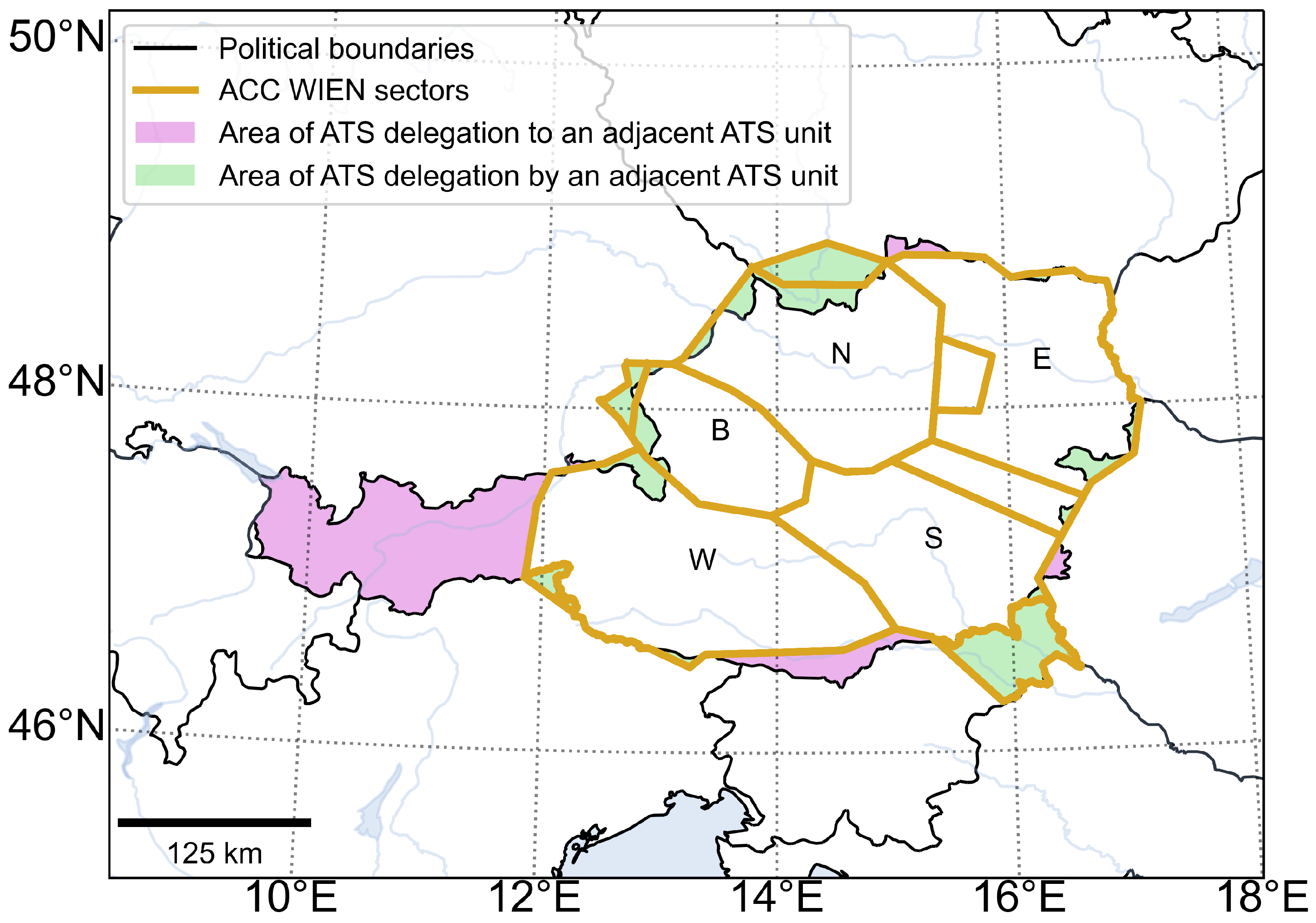
For AIRAC cycle 1806, the Austrian airspace under the control of the Wien Area Control Centre (ACC WIEN) is shown in Figure 4. It is divided into five geographical regions (B, E, N, S, and W), and each region into five vertical layers:

• ACC WIEN B: B1, B2, B3, B4, and B5;
• ACC WIEN E: E1, E2, E3, E4, and E5;
• ACC WIEN N: N1, N2, N3, N4, and N5;
• ACC WIEN S: S1, S2, S3, S4, and S5; and
• ACC WIEN W: W1, W2, W3, W4, and W5.

In total, 38 elementary volumes are used to define this airspace, which leads to near 60 possible different ATC sectors and 190 different sector configurations. For instance, sector configuration 10A1 (the one initially scheduled for the time interval from $T_P$ to $T_P+1.5$ h) is formed by ten ATC sectors: B15, E13, E45, N12, N35, S12, S35, W12, W3, and W45, where, for example, W45 consists of all the elementary volumes taken from W4 and W5, and so forth.

5.2. Weather Scenario

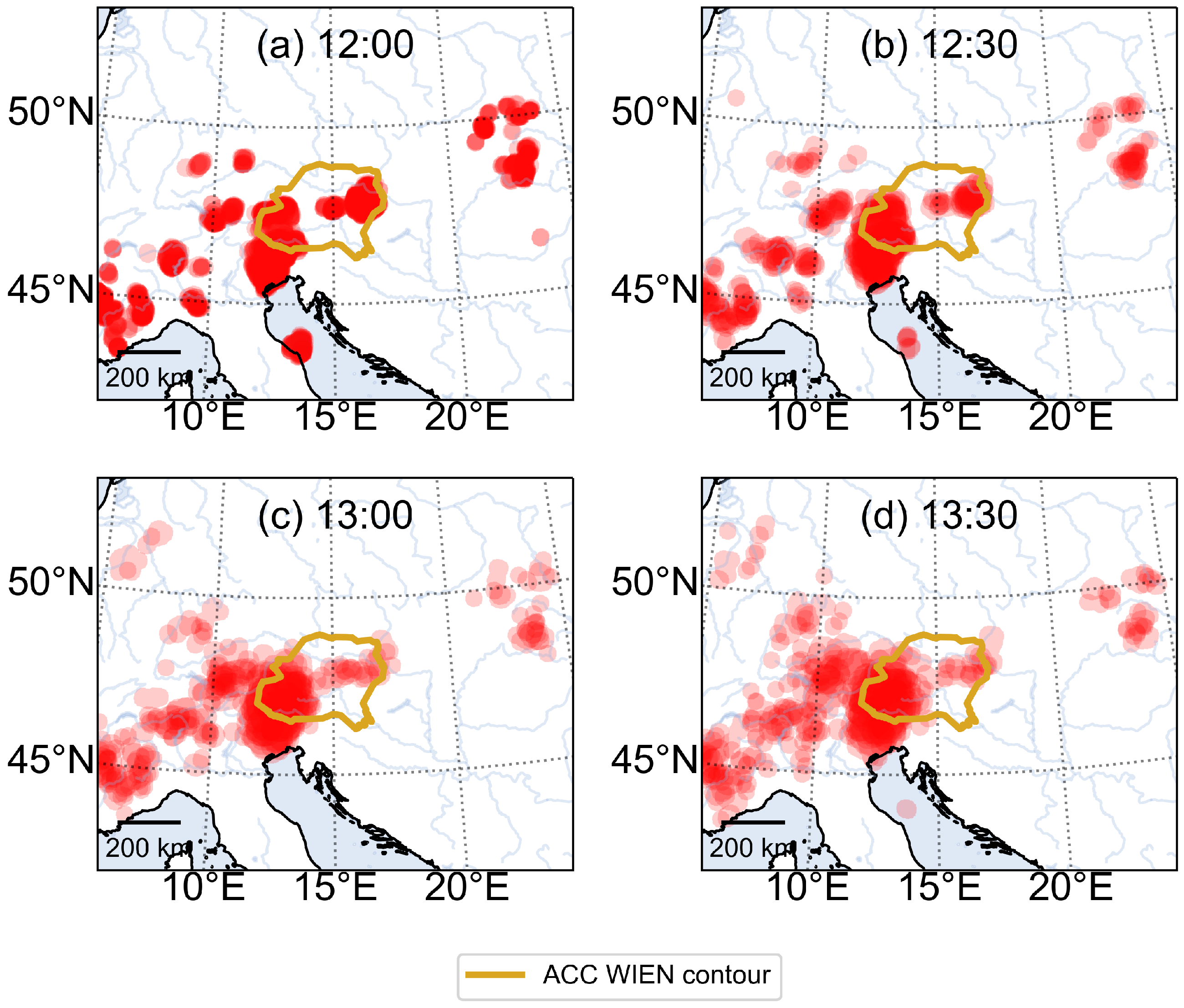
The nowcast employed in this application is the one generated at 12:00 with time horizon until 13:30. The ensemble nowcast is formed by 15 statistically independent members. Each member has been interpolated every 5 min and processed according to what has already been described. An example, corresponding to the prediction for 12:00, 12:30, 13:00, and 13:30, is depicted in Figure 5. The no-fly zones are represented in red. The transparency in a particular location represents the number of members that predict a storm cell to be in that very location (more members, less transparent).

The wind and temperature forecast is assumed to be deterministic as mentioned in Section 2.1. In particular, the forecast is obtained from the latest released ECMWF-EPS, that is, the one generated at 00:00. It has been interpolated every 15 min.

5.3. Traffic Scenario

The historical traffic data were retrieved from Eurocontrol’s R&D Data Archive. For the trajectory predictor used in this application, we considered the following filed data: the positions of airborne aircraft at 12:00, the nominal take-off times, and the nominal trajectories to be followed are the ones given in their flight plans. The resulting predicted trajectories are the input for the probabilistic methodologies presented in this paper. In addition, we used actual traffic data for a comparative exercise in Section 6.1.1. The corresponding executed trajectories are also extracted from Eurocontrol’s R&D Data Archive.

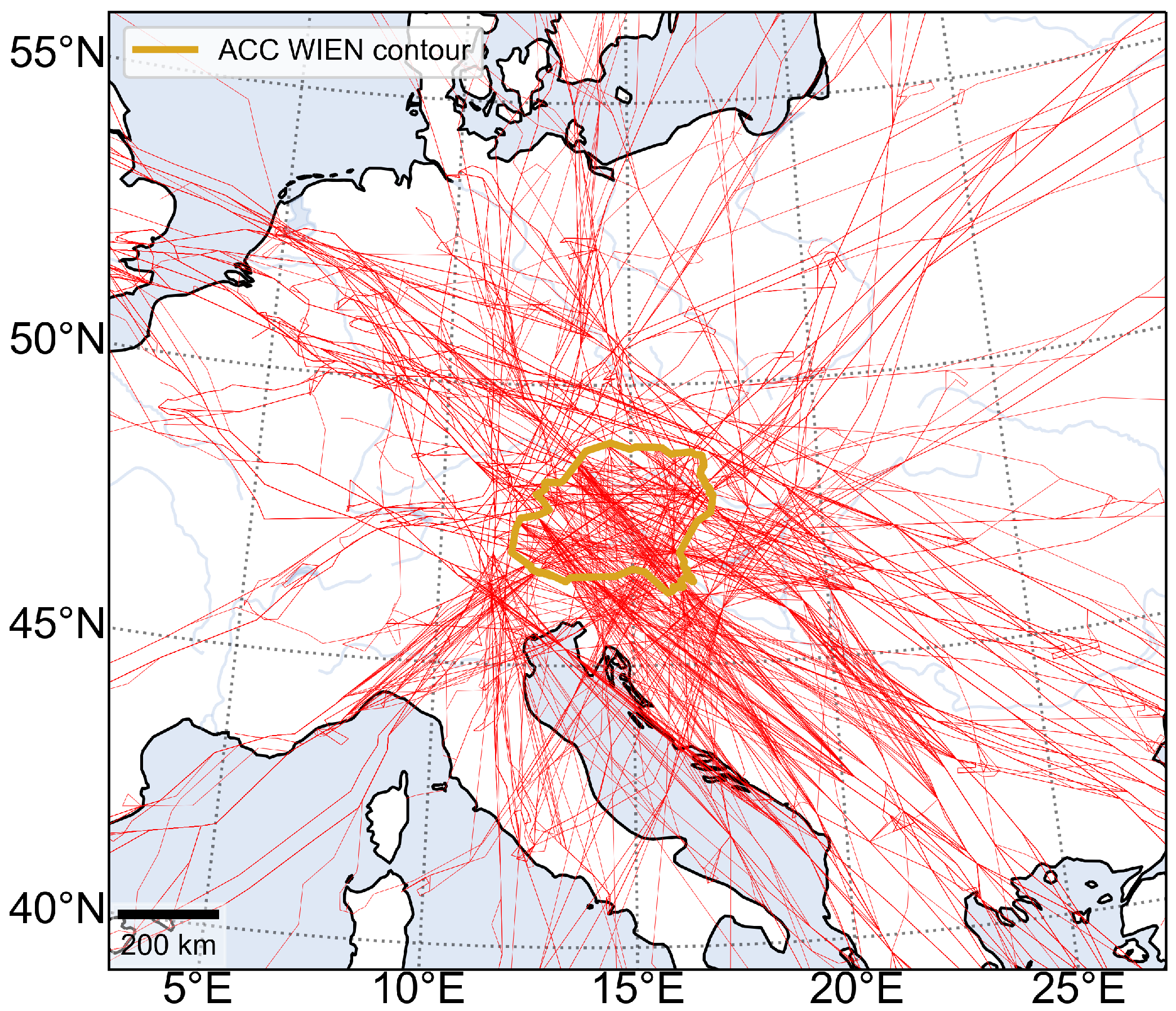
The traffic considered in this application (a package with 1096 flights, see Figure 6) consists of aircraft airborne at 12:00 (486 flights) or expected to take off in the next 90 min (610 flights), which plan to cross the Austrian airspace plus a surrounding area of 50 NM. The surrounding area was included to take into account those aircraft that may be deviated into the airspace of interest because of the convective weather.

In this way, it is contemplated the possibility that some aircraft, flying close to the airspace of interest, may be deviated into it because of the convective weather.

5.4. Additional Technical Enablers

The results obtained in this paper also rely on two supporting technical enablers:

• A probabilistic trajectory predictor (TP) to generate, for each flight, an ensemble of 4D trajectories that provides a measure of the trajectory uncertainty, each trajectory avoiding the storm cells encountered along the way. In this paper, the TP based on the predictor presented by Franco et al. in [40] is used. It considers spatiotemporal variations of the wind and the air temperature, and, more importantly, the storm forecast uncertainty, including the uncertainty in the size, location, and height of the individual storm cells. For each simulated scenario, the tool returns a trajectory that laterally avoids those no-fly regions closer than a minimum horizontal distance of 13.5 NM [32] and a minimum vertical distance of 5000 ft [41]. A visibility graph is computed, with a starting point at a total distance of 40 NM from the threatening convective cloud [42]; then, the circumnavigation is computed using the Dijkstra’s algorithm and BADA 3.12. For more details, see [40].
• A calculator of ASCR values corresponding to any sector s, period j, and weather ensemble member k. In this paper, the approach adopted is based on [43], where ASCRs are calculated from the ratio of intersecting storms volume to sector volume. Moreover, to avoid over-optimistic ASCRs in those sectors comprising the highest layer, whose upper limit value is FL660, their volumes are determined by using as top limit the maximum altitude reached by all the flights under study.

6. Results and Discussion

The results are presented as follows. First, a preliminary analysis is conducted in Section 6.1. Second, the probabilistic entry and occupancy counts are examined in Section 6.2. Finally, the sector congestion is analyzed via the ROL values and the overload risks in Section 6.3.

6.1. Input Analysis

6.1.1. Traffic Scenario Analysis

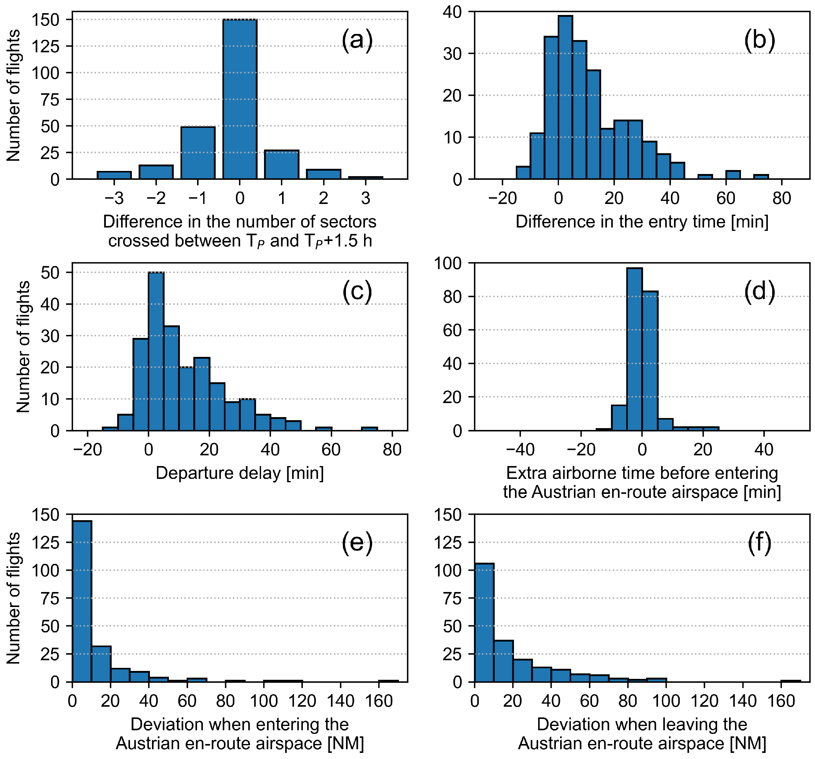
The first analysis consists of a high-level comparison between the actual and planned trajectories from the traffic set described in Section 5.3. Illustrated in Figure 7, there are several remarkable differences. Figure 7a shows the difference—reality minus plan—in the number of sectors from configuration 10A1 crossed between $T_P$ and $T_P$ + 1.5 h for all the flights, except for those where neither planned nor actual trajectories entered the airspace of interest. In most cases, there is no difference in the number—although the sectors are not necessarily the same—but a deviation of up to three sectors in a non-negligible amount of flights is observed. Among the flights counted in Figure 7a, there are 45 flights that, despite being expected in the Austrian en-route airspace during the specified time interval, avoided it, and 3 flights that, despite not being expected, penetrated it. Without them, the difference in the entry time of the remaining flights is examined (Figure 7b), and the majority of flights are found to enter later than scheduled. This finding can be reasonably linked to the departure delays (Figure 7c); however, the shortcuts and circumnavigations upstream are to be considered because they affect the extra time before entering the Austrian en-route airspace (Figure 7d), and they determine which sectors are finally crossed. Such spatial deviations can be quantified by calculating the distance between the planned and actual trajectories. In Figure 7e,f they are quantified at the entry and exit points of the en-route airspace.

Not all the aforementioned upstream deviations are due to the meteorological event of interest. In general, they are due to all sorts of regulations and pilot decisions, which makes it difficult to compare planned and real traffic demand. This is why, in our study, the probabilistic prediction given by the ensemble of trajectories—a total of 87,615 trajectories—simulated under an isolated environment, is solely compared to the prediction given by the FPLs.

6.1.2. Reduced Weather Capacity

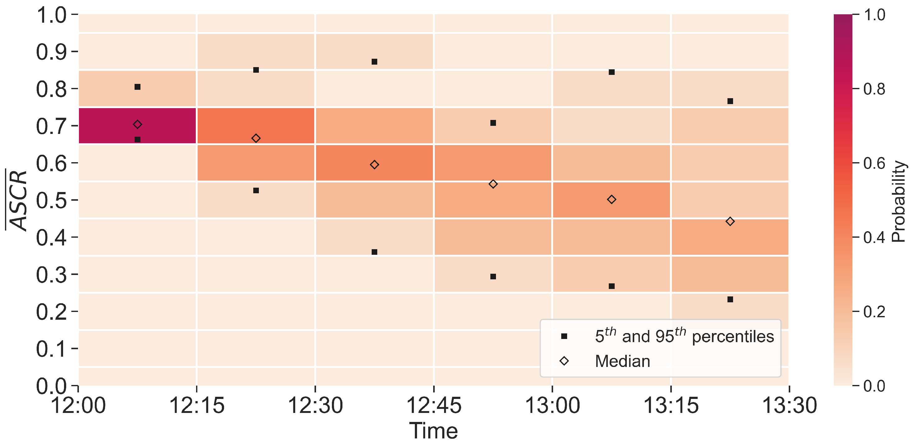
An example of the results of capacity reduction obtained with the method described in Section 5.4, for sector B15, is shown in Figure 8. Without loss of generality, the mean ASCR is presented in periods of 15 min ($\overline{ASCR}\_15$). The temporal distribution reflects that the situation becomes worse through time, not only in terms of uncertainty, but the median decreases as well (from 0.7 to 0.45, approximately). One can see a clear connection with the weather evolution shown in Figure 5.

Regarding the congestion assessment, the ASCRs must be expressed in time periods of one hour, as this is how the nominal MV is expressed. Specifically, the nominal MV of sector B15 is 46 aircraft per hour.

Table 2. Percentiles of hourly mean ASCR and hourly weather-dependent MV for sector B15.

Period	$\overline{\mathit{ASCR}}\_60$			$\mathit{Wx}\_\mathit{MV}$
	${\mathit{Z}}_{\mathbf{5}}$	${\mathit{Z}}_{\mathbf{50}}$	${\mathit{Z}}_{\mathbf{95}}$	${\mathit{Z}}_{\mathbf{5}}$	${\mathit{Z}}_{\mathbf{50}}$	${\mathit{Z}}_{\mathbf{95}}$
12:00–13:00	0.460	0.617	0.807	21.2	28.4	37.1
12:15–13:15	0.362	0.571	0.767	16.7	26.3	35.3
12:30–13:30	0.295	0.522	0.756	13.6	24.0	34.8

presents the probabilistic ASCR and the probabilistic reduced MV at hourly rate every 15 min, $\overline{ASCR}\_60$ and $Wx\_MV$. The probabilistic information of each period is summarized in three columns: one for the 5th percentile ($Z_5$), another one for the 50th percentile ($Z_{50}$), and a third one for the 95th percentile ($Z_{95}$).

6.2. Entry and Occupancy Counts

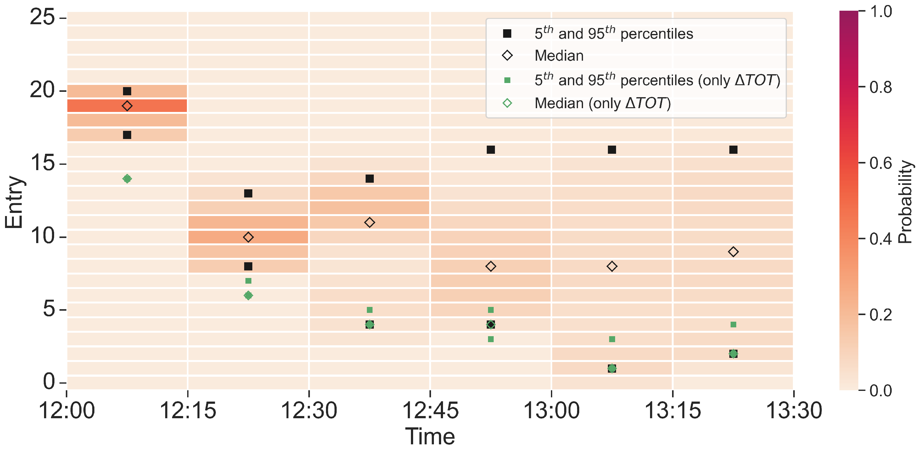
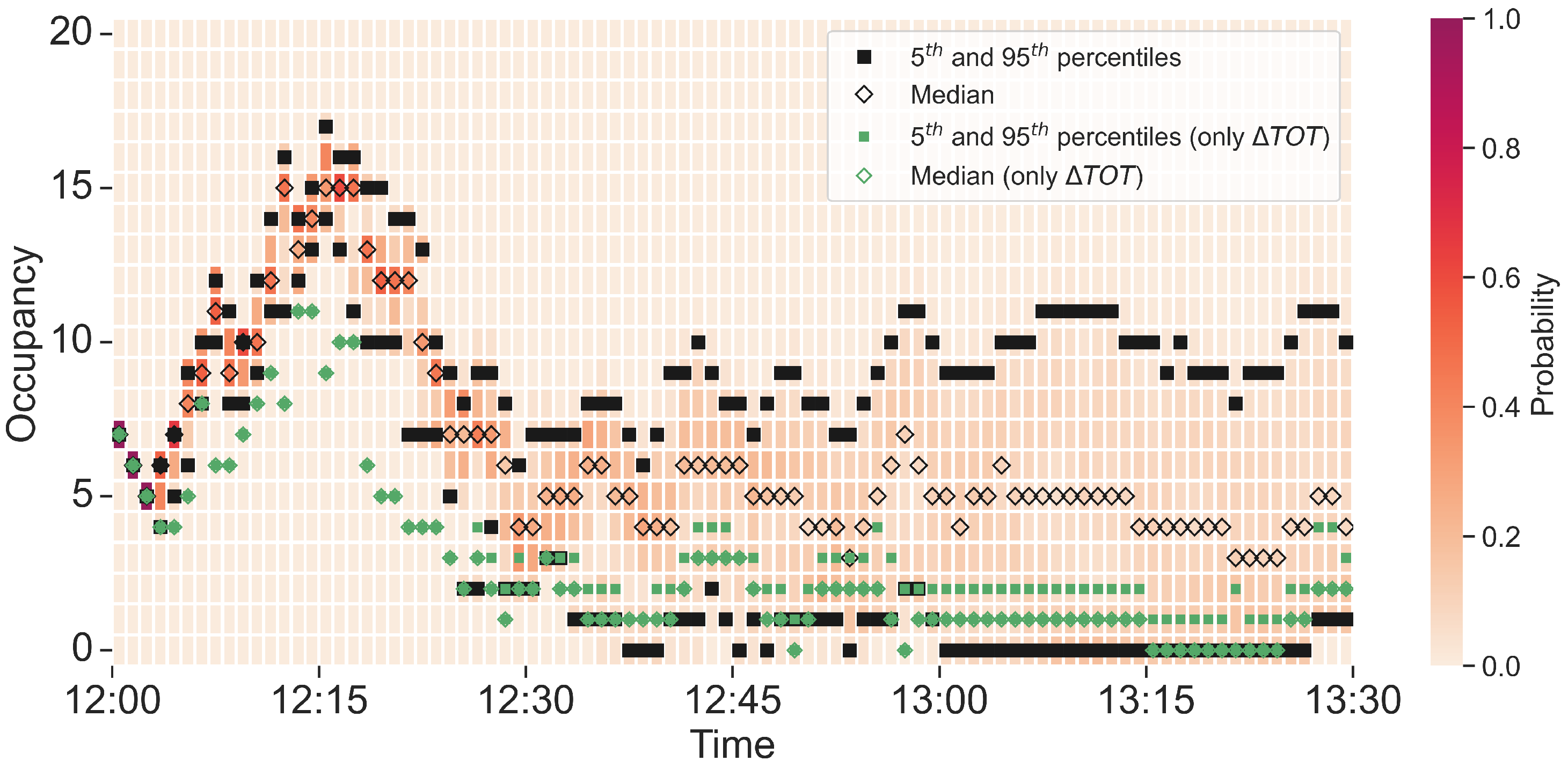
After calculating the entry and exit times of the predicted trajectories, the probabilistic entry and occupancy counts are determined as described in Section 3.3 and Section 3.4, for the values of $\Delta t_{Skip-In}=1$ min and $\Delta t_{Skip-Out}=30$ min. Then, their temporal distributions are visualized in charts where the probability information is conveyed through discrete heatmaps (the warmer the color, the more probable the count). These heatmaps also contain markers of the 5th and 95th percentiles (represented as black-filled squares), and the median (represented as a black empty diamond). In particular, results for sector B15 are presented next.

The entry counts are visualized in Figure 9. With respect to the values of $\delta t$ and $\Delta t$, the entry counts are normally monitored at hourly rate every 20 min ($\delta t=20$ min, $\Delta t=60$ min); nonetheless, to achieve a clearer idea of the temporal distribution of the counts, they are here displayed in time bins of 15 min ($\delta t=\Delta t=15$ min). Several observations about the results can be made: (1) the median takes values between 8 and 19, being the first period the most demanded one; (2) at the beginning, the deviation of the 5th and 95th percentiles from the median is only one to two aircraft, whereas the deviation is of seven aircraft at the end, and up to eight aircraft in between, indicating that uncertainty in entry counts grows over time (as expected); (3) the median is not exactly at the center of the 5th and 95th percentiles, i.e., the distributions are not symmetrical.

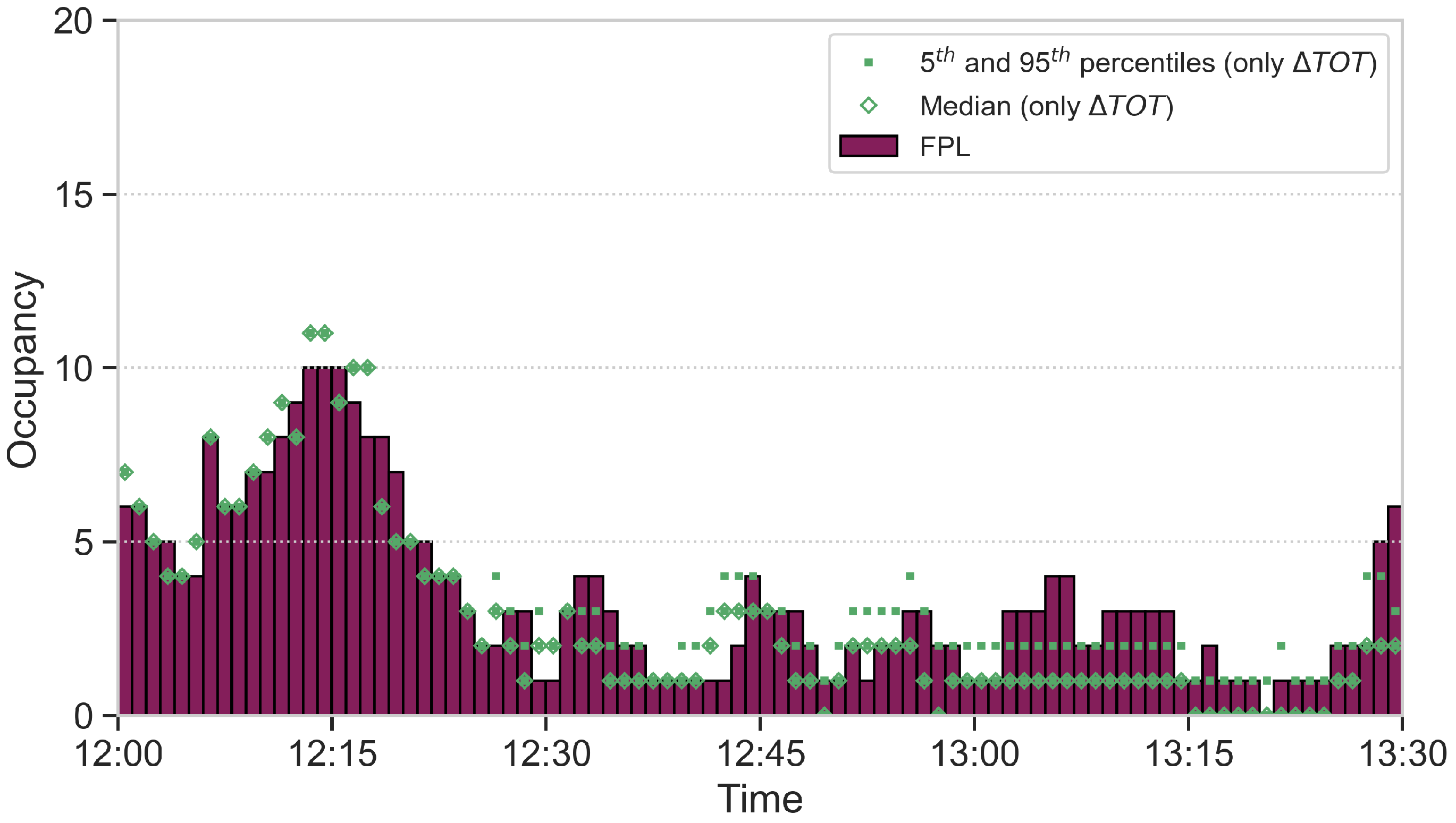
The occupancy counts are visualized in Figure 10. Here, the counts are viewed in time bins of 1 minute ($\delta t=\Delta t=1$ min) and in a window of 1.5 h. The results indicate that the median takes values between 3 and 15, being the time intervals 12:12–12:13 and 12:15–12:18 the most demanded ones. This peak is related to the fact that the first period is when more aircraft enter sector B15 (see Figure 9). Analogous comments to those made for the entry counts can be made here as well, where the dispersion is zero during the first minutes and up to six aircraft afterwards.

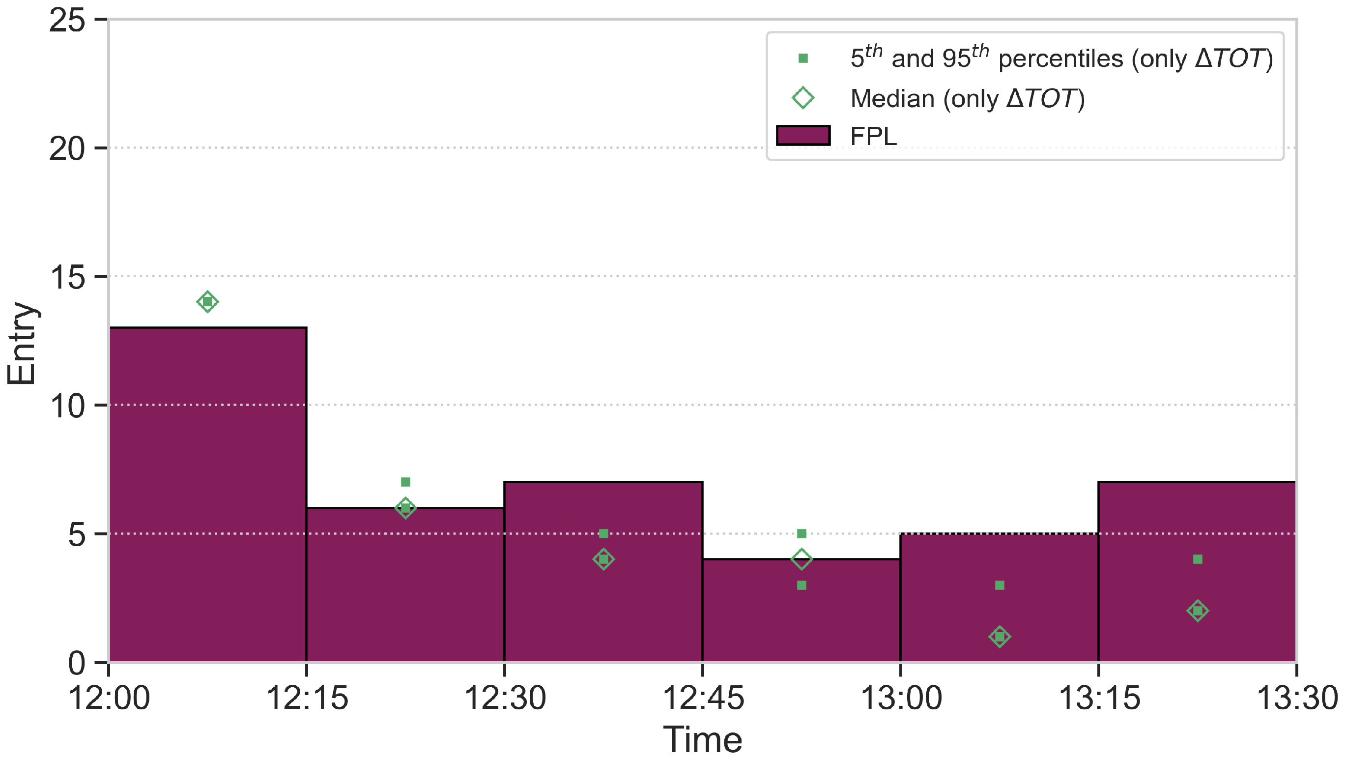
Note that Figure 9 and Figure 10 contain some data in green corresponding to a hypothetical case without storm, so that the only source of uncertainty would be the one that in the take-off time. Thus, one can compare the magnitude of the uncertainty in the initial conditions with the magnitude of the combination of the two sources incorporated in this work. See that the uncertainty tied to the take-off time is zero at the beginning and grows with time overall, but remains smaller than the combined uncertainty at all times. In addition, observe that the counts including the presence of the storm can strongly differ from the values obtained with only the take-off time uncertainty (which take values around the demand dictated by the flight plan, as shown in Figure 11 and Figure 12). For all these reasons, one concludes that the consideration of the spatiotemporal uncertainty sources is needed (as compared to only considering the temporal uncertainty) and that, as expected, the impact of the storm is significant in terms of traffic loads.

6.3. Congestion

Once the demand and capacity have been determined, the relative overload is calculated as described in Section 4.2. The entry relative overload (E-ROL) is obtained with the hourly entry count and the hourly reduced MV. The outcome for all the sectors of sector configuration 10A1 are gathered in

Table 3. Percentiles of the hourly entry ROL values (E-ROL).

Sector	12:00–13:00			12:15–13:15			12:30–13:30
	${\mathit{Z}}_{\mathbf{5}}$	${\mathit{Z}}_{\mathbf{50}}$	${\mathit{Z}}_{\mathbf{95}}$	${\mathit{Z}}_{\mathbf{5}}$	${\mathit{Z}}_{\mathbf{50}}$	${\mathit{Z}}_{\mathbf{95}}$	${\mathit{Z}}_{\mathbf{5}}$	${\mathit{Z}}_{\mathbf{50}}$	${\mathit{Z}}_{\mathbf{95}}$
B15	1.34	1.70	1.94	0.91	1.39	1.83	0.83	1.44	1.93
W45	0.19	0.21	0.25	0.14	0.16	0.19	0.16	0.19	0.24
W3	0.84	1.09	1.27	0.56	0.83	1.31	0.43	0.80	1.51
W12	1.44	2.11	2.36	1.51	2.04	2.54	1.84	2.34	3.16
S35	0.44	0.48	0.55	0.37	0.44	0.50	0.43	0.53	0.61
S12	0.68	0.85	1.02	0.54	0.80	1.0	0.67	0.89	1.15
E45	0.29	0.30	0.31	0.31	0.32	0.35	0.27	0.32	0.36
E13	0.65	1.03	1.34	0.51	0.71	0.93	0.50	0.64	0.89
N35	0.42	0.45	0.53	0.44	0.49	0.59	0.40	0.50	0.65
N12	0.82	0.97	1.27	0.72	0.92	1.17	0.82	1.06	1.35

.

In order to assess the congestion and determine the overload risk, the probabilistic double-entry criterion introduced in Section 4.3 is applied to the values in Table 3. The results are visualized in Figure 13. It is immediate to see that six of the sectors are affected by the meteorological event, specifically sectors B15, W3, W12, S12, E13, and N12. Sectors B15 and W12 are clearly predicted to be overloaded (in red) due to the big convection cell shown in Figure 5; therefore, ATFCM measures are needed. Sector W3 is overloaded during the first period, while the overload risk in the other two periods is very high (in orange) and, consequently, alternate actions should be prepared. The case of sector N12 is similar, with the overload during the last period. Other sectors that present overload issues are E13, which is red during the first period, and S12, which is orange during the third period. Beforehand, one could conclude that weather would strongly impact the sector configuration 10A1 (at all time periods, there are sectors with an unacceptable risk). In fact, the sector configuration was modified that day up to four times, trying others with nine or ten sectors.

Comparing the values in Table 3 with the resulting color in Figure 13, it can be observed that there are situations where the risk is categorized more severely just because of the uncertainty. For instance, for sector N12, a deterministic criterion considering only the median would return a high risk during the first period, a high risk during the second period, and a very high risk during the third period. However, with a probabilistic criterion, the overload risk increases to very high, very high, and unacceptable, respectively.

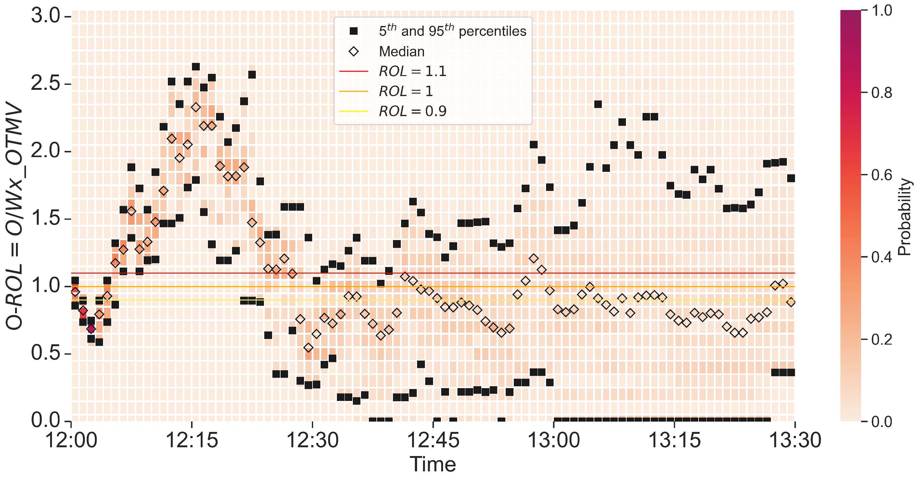
To complement the previous results, sectors can be analyzed further by checking different visualizations. For example, sector B15 is examined in Figure 14 by plotting the evolution of its occupancy relative overload (O-ROL). Despite starting well, the occupancy rapidly exceeds the sustained OTMV for about 20 min. Then, it falls generally below the threshold $ROL=1.1$, although the dispersion increases dramatically.

7. Conclusions

The content of this paper is placed within the framework of the development of ATM-oriented methodologies to deal with weather uncertainty. In particular, the research conducted in this work responds to the necessity declared by EUROCONTROL to improve the predictability of the traffic situation, especially in the short term. Because adverse weather is known to be a very uncertain and disruptive phenomenon, its modeling and integration into the air traffic management are of great importance.

Our innovation is the probabilistic methodologies to predict sector demand and sector congestion, including a new probabilistic criterion to assess the risk of sector overload. Compatible with other technical enablers different from those in Section 5.4, these methodologies aim to improve the ATM efficiency by supporting the FMPs in taking anticipated, appropriate, and timely tactical flow measures under adverse weather; that is, to allow for a better-informed decision-making process. The potential impact is ultimately to reduce flight delays and improve passenger journeys.

In this paper, the approach has been based on considering spatiotemporal uncertainties, namely, the one inherent to meteorology forecast and the uncertainty in the take-off time. Each uncertainty has been modeled via an ensemble approach, in which a representative set of possible outcomes (i.e., members) is generated. The time horizon has been 1.5 h; therefore, the weather ensemble is built around a probabilistic nowcast. To create the take-off time ensemble, for flights still on ground at the prediction time, the estimated take-off time resulting from the flight plan is deviated based on experimental results.

The output of the probabilistic trajectory predictor is, for each flight, an ensemble of 4D avoidance trajectories that laterally avoid the non-static storm cells and reattach to the originally planned trajectory. The provision of probabilistic aircraft trajectories in the form of an ensemble of deterministic trajectories is a needed input for the methodologies developed in this paper. Although one particular trajectory predictor has been used in this paper, other trajectory predictors could be considered as well. For example, probabilistic adaptations of the predictor currently at use by the traffic flow managers.

Methodologies to calculate probabilistic demand and congestion have been presented. These methodologies assume that the meteorological uncertainty is fully correlated for the different aircraft, whereas the uncertainty in the initial conditions are statistically independent from one flight to another. In the future, the latter assumption may be relaxed to consider, for example, situations in which different aircraft departing from the same airport experience similar delays.

The demand and congestion methodologies have been tested in a realistic case study, a historical situation with significant convection over the Austrian upper airspace. The graphical visualization of uncertainty is not trivial at all. It must be conveyed in such a way that it does not result too disruptive for non-trained staff, yet enables the decision-making process. In this work, the choice has been the use of heatmaps. Moreover, a new color code has been introduced for the assessment of sector overload risks. This code is a natural extension of the deterministic criterion used nowadays. It considers the shape of the statistical distributions through the median and the 95th percentile. The inclusion of this high-value percentile seeks to penalize the possibility of encountering worse scenarios.

One task left for future work is the implementation of what-if analyses to see, for example, the effect of changing sector configurations. This ability is of great interest when determining the ATFCM measures that should be implemented, as they provide an estimation of their impact. Another future development is the identification of the traffic flows that introduce more dispersion in the counts. This is essential for the decision-making process, because the level of uncertainty can become unapproachable sometimes. Finally, it is interesting to extend the methodology to larger temporal horizons. In such extended temporal scale, convection-permitting EPS are the best weather forecasts available nowadays. Since their ability to predict the storm cells is very limited because of the spatial and temporal resolutions, a different approach is needed. A promising plan is to use historical traffic situations and to find statistical correlations between the convection indicators and lateral, longitudinal, and vertical deviations.

References

1. Niarchakou, S.; Sfyroeras, M. ATFCM Users Manual; Technical Report; EUROCONTROL Network Manager Directorate: Brussels, Belgium, 2022. [Google Scholar]
2. Taszarek, M.; Allen, J.; Hoogewind, K.; Brooks, H. Severe convective storms across Europe and the United States. Part II: ERA5 environments associated with lightning, large hail, severe wind, and tornadoes. J. Clim. 2020, 33, 10263–10286. [Google Scholar] [CrossRef]
3. NOAA. Severe Weather 101: Thunderstorm Types. Available online: https://www.nssl.noaa.gov/education/svrwx101/thunderstorms/types/ (accessed on 3 February 2024).
4. Berberi, L. Maltempo a Milano, la Grandine Buca il Muso Dell’aereo Diretto a New York: Volo Dirottato a Roma. Corriere della Sera. 24 July 2023. Available online: https://www.corriere.it/economia/consumi/23_luglio_24/maltempo-milano-grandine-buca-muso-dell-aereo-diretto-new-york-volo-dirottato-roma-8495fe2c-2a32-11ee-84ae-fdab1efa7b6b.shtml (accessed on 25 July 2023).
5. Dalmau, R. Predicting the likelihood of airspace user rerouting to mitigate air traffic flow management delay. Transp. Res. Part C Emerg. Technol. 2022, 144, 103869. [Google Scholar] [CrossRef]
6. Xu, Y.; Prats, X.; Delahaye, D. Synchronised demand-capacity balancing in collaborative air traffic flow management. Transp. Res. Part C Emerg. Technol. 2020, 114, 359–376. [Google Scholar] [CrossRef]
7. Niarchakou, S.; Sfyroeras, M. ATFCM Operations Manual; Technical Report; EUROCONTROL Network Manager Directorate: Brussels, Belgium, 2022. [Google Scholar]
8. EUROCONTROL Performance Review Commission. Technical Note on En Route Capacity; Technical Report; EUROCONTROL Performance Review Commission: Brussels, Belgium, 2020; Available online: https://www.eurocontrol.int/sites/default/files/2020-12/eurocontrol-prc-technical-note-en-route-capacity-11122020.pdf (accessed on 17 March 2024).
9. EUROCONTROL Network Manager. Demonstration Report (DEMOR) PJ24 NCM; Technical Report; EUROCONTROL Network Manager: Brussels, Belgium, 2019; Available online: https://www.sesarju.eu/sites/default/files/documents/projects/FPR/733021_PJ24_D1.2_Demonstration%20Report.pdf (accessed on 17 March 2024).
10. Meyn, L. Probabilistic methods for air traffic demand forecasting. In Proceedings of the AIAA Guidance, Navigation, and Control Conference, Monterrey, CA, USA, 5–8 August 2002. [Google Scholar]
11. Suarez, N.; Grcia-Ovies, I.; Zheng, D.; Boucquey, J. Assessing the viability of an occupancy count prediction model. In Proceedings of the 7th SESAR Innovation Days, Belgrade, Serbia, 28–30 November 2017. [Google Scholar]
12. Steiner, M.; Bateman, R.; Megenhardt, D.; Liu, Y.; Pocernich, M.; Krozel, J. Translation of Ensemble Weather Forecasts into Probabilistic Air Traffic Capacity Impact. Air Traffic Control Q. 2010, 18, 229–254. [Google Scholar] [CrossRef]
13. Gonze, F.; Jungers, R.; Koyuncu, E. Probabilistic Traffic Demand Models. Technical Report; COPTRA Project. 2017. Available online: https://ec.europa.eu/research/participants/documents/downloadPublic?documentIds=080166e5b4b387fb&appId=PPGMS (accessed on 17 March 2024).
14. Zobell, S.; Wanke, C.; Song, L. Probabilistic airspace congestion management. In Proceedings of the 12th Conference on Aviation, Range, and Aerospace Meteorology, American Meteorological Society, Atlanta, GA, USA, 30 January–2 February 2006. [Google Scholar]
15. Jardines, A.; Soler, M.; García-Heras, J. Estimating entry counts and ATFM regulations during adverse weather conditions using machine learning. J. Air Transp. Manag. 2021, 95, 102109. [Google Scholar] [CrossRef]
16. Jardines, A.; Soler, M.; García-Heras, J. Data-driven occupancy prediction in adverse weather conditions using thunderstorm and traffic observations. In Proceedings of the 9th SESAR Innovation Days, Athens, Greece, 2–6 December 2019. [Google Scholar]
17. Abecassis, A.; Delahaye, D.; Idan, M. A machine learning framework to predict general aviation traffic counts: A case study for Nice Cote D’Azur Terminal Control Center. In Proceedings of the 12th SESAR Innovation Days, Budapest, Hungary, 5–8 December 2022. [Google Scholar]
18. Valenzuela, A.; Franco, A.; Rivas, D.; García-Heras, J.; Soler, M. Effects of reducing wind-induced trajectory uncertainty on sector demand. In Proceedings of the 7th SESAR Innovation Days, Belgrade, Serbia, 28–30 November 2017. [Google Scholar]
19. Valenzuela, A.; Franco, A.; Rivas, D. An approach to en-route sector demand prediction subject to thunderstorms. In Proceedings of the 13th USA/Europe ATM Research and Development Seminar, Vienna, Austria, 17–21 June 2019. [Google Scholar]
20. Andrés, E.; García-Heras, J.; González, D.; Soler, M.; Valenzuela, A.; Franco, A.; Nunez-Portillo, J.; Rivas, D. Probabilistic analysis of air traffic in adverse weather scenarios. In Proceedings of the ICRAT, Tampa, FL, USA, 19–23 June 2022. [Google Scholar]
21. Lemetti, A.; Polishchuk, T.; Polishchuk, V.; Valenzuela, A.; Franco, A.; Nunez-Portillo, J.; Rivas, D. Probabilistic Analysis of Airspace Capacity in Adverse Weather Scenarios. In Proceedings of the 12th SESAR Innovation Days, Budapest, Hungary, 5–8 December 2022. [Google Scholar]
22. Schmid, F.; Agersten, S.; Bañón Peregrín, L.M.; Buzzi, M.; Atencia, A.; De Coning, E.; Kann, A.; Moseley, S.; Reyniers, M.; Wang, Y.; et al. Conference report: Fourth European nowcasting conference. Meteorol. Z. 2023, 32, 83–87. [Google Scholar] [CrossRef]
23. World Meteorological Organization. Nowcasting/Very Short-Range Forecasting. Available online: https://space.oscar.wmo.int/applicationareas/view/2_3_nowcasting_very_short_range_forecasting (accessed on 12 March 2024).
24. Basora, L.; Courchelle, V.; Bedouet, J.; Dubot, T. Occupancy peak estimation from sector geometry and traffic flow data. In Proceedings of the 8th SESAR Innovation Days, Salzburg, Austria, 3–7 December 2018. [Google Scholar]
25. Comeford, D.; Granada, S.; Johnson, W.; Battiste, V.; Dao, A.; Brandt, S. NASA/TM-2009-215384 Pilots’ Weather-Related Decision Making: Results from a Workshop and a Survey; Technical Report; Ames Research Center: Moffett Field, CA, USA, 2009. [Google Scholar]
26. Chan, W.; Refai, M.; DeLaura, R. An approach to verify a model for translating convective weather information to air traffic management impact. In Proceedings of the 7th AIAA ATIO, Belfast, UK, 18–20 September 2007. [Google Scholar]
27. Avjian, R.; Dehn, J.; Stobie, J. NextGen trajectory based integration of grid-based weather avoidance fields. In Proceedings of the ARAM Special Symposium on Weather-ATM Integration, Washington, DC, USA; 2011. [Google Scholar]
28. Rhoda, D.; Boorman, B.; Bouchard, E.; Pawlak, M. Commercial aircraft encounters with thunderstorms in the Memphis terminal airspace. In Proceedings of the 9th ARAM, Orlando, FL, USA, 12–16 September 2000. [Google Scholar]
29. Lin, Y.; Balakrishnan, H. Prediction of terminal-area weather penetration based on operational factors. Transp. Res. Rec. 2013, 2400, 45–53. [Google Scholar] [CrossRef]
30. Bowler, N.; Pierce, C.; Seed, A. STEPS: A probabilistic precipitation forecasting scheme which merges an extrapolation nowcast with downscaled NWP. Q. J. R. Meteorol. Soc. 2006, 132, 2127–2155. [Google Scholar] [CrossRef]
31. Reinoso-Rondinel, R.; Troemel, S.; Simmer, C.; Rempel, M. Radar-Based Ensemble Nowcasting: Predictability Analysis. Technical Report. 2021. Available online: https://essopenarchive.org/doi/full/10.1002/essoar.10505879.1 (accessed on 12 March 2024).
32. DeLaura, R.; Evans, J. An Exploratory Study of Modeling Enroute Pilot Convective Storm Flight Deviation Behaviour. In Proceedings of the 12th Conference on Aviation, Range and Aerospace Meteorology, American Meteorological Society, Atlanta, GA, USA, 30 January–2 February 2006. [Google Scholar]
33. Dalmau, R.; Bellerini, H.; Belkoura, S.; Wangnick, S. An explainable machine learning approach to improve take-off time prediction. J. Air Transp. Manag. 2021, 95, 102090. [Google Scholar] [CrossRef]
34. Sale, S. Development of a Computer Based Airspace Sector Occupancy Model. Ph.D. Thesis, Virginia Polytechnic Institute and State University, Blacksburg, VA, USA, 1998. Available online: https://vtechworks.lib.vt.edu/items/e304ba09-b21f-42a1-8578-4880e7215562/full (accessed on 29 January 2024).
35. Mood, A.; Graybill, A.; Boes, D. Introduction to the Theory of Statistics; McGraw-Hill, Inc.: New York, NY, USA, 1974. [Google Scholar]
36. Grinstead, C.; Snead, J. Introduction to Probability; American Mathematical Society: Providence, RI, USA, 1997. [Google Scholar]
37. Gilles, S. The Shapely User Manual. 2020. Available online: https://shapely.readthedocs.io/en/stable/manual.html#id25 (accessed on 27 September 2020).
38. Wiki. GEOS. 2021. Available online: https://trac.osgeo.org/geos (accessed on 16 June 2021).
39. Davis, M. JTS Technical Specifications. 2003. Available online: https://github.com/locationtech/jts/raw/master/doc/JTS%20Technical%20Specs.pdf (accessed on 27 September 2020).
40. Franco, A.; Valenzuela, A.; Rivas, D.; Sacher, D.; Lang, J.; Hauf, T. A Probabilistic Storm Avoidance Concept for En-Route Flight. In Proceedings of the 10th SESAR Innovation Days, SESAR Joint Undertaking, Online, 7–10 December 2020. [Google Scholar]
41. SKYbrary. Weather Radar: Storm Avoidance. 2021. Available online: https://skybrary.aero/articles/weather-radar-storm-avoidance (accessed on 14 October 2021).
42. Marconnet, D.; Norden, C.; Vidal, L. Optimum use of weather radar. Saf. First 2016, 22, 22–23. [Google Scholar]
43. Russell, C. Predicting airspace capacity impacts using the consolidated storm prediction for aviation. In Proceedings of the 10th AIAA ATIO Conference, Forth Worth, TX, USA, 13–15 September 2010. [Google Scholar]
Figure 1. Workflow for producing uncertainty-based traffic forecasts of interest to FMPs.
Aerospace 11 00240 g001
Figure 2. Combined two-stage approach to perform prediction of sector demand and sector congestion.
Aerospace 11 00240 g002
Figure 3. Evolution from the deterministic single-entry criterion (left) to the probabilistic double-entry criterion (right).
Aerospace 11 00240 g003
Figure 4. Geographical description of the Austrian airspace.
Aerospace 11 00240 g004
Figure 5. Nowcast generated at 12:00, prediction for four different instants (ad).
Aerospace 11 00240 g005
Figure 6. Planned trajectories of the flights considered in the application.
Aerospace 11 00240 g006
Figure 7. Comparative analysis of the deviations (af) between the actual and planned trajectories of the selected flights.
Aerospace 11 00240 g007
Figure 8. Mean ASCR ( A S C R ¯ _ 15 ) through time for sector B15.
Aerospace 11 00240 g008
Figure 9. Probabilistic entry counts through time for sector B15.
Aerospace 11 00240 g009
Figure 10. Probabilistic occupancy counts through time for sector B15.
Aerospace 11 00240 g010
Figure 11. Entry counts for the FPLs through time for sector B15.
Aerospace 11 00240 g011
Figure 12. Occupancy counts for the FPLs through time for sector B15.
Aerospace 11 00240 g012
Figure 13. Overload risks for sector configuration 10A1.
Aerospace 11 00240 g013
Figure 14. Occupancy ROL (O-ROL) through time for sector B15.
Aerospace 11 00240 g014