Author Contributions
Conceptualization, A.K., S.K., E.F. and V.K.; methodology, E.F. and S.K.; software, E.F.; validation, E.F.; formal analysis, E.F.; investigation, E.F. and S.K.; resources, E.F. and S.K.; data curation, E.F.; writing—original draft preparation, E.F. and S.K.; writing—review and editing, E.F., S.K., A.K. and V.K.; visualization, E.F.; supervision, A.K., S.K. and V.K.; project administration, A.K. and V.K. All authors have read and agreed to the published version of the manuscript.
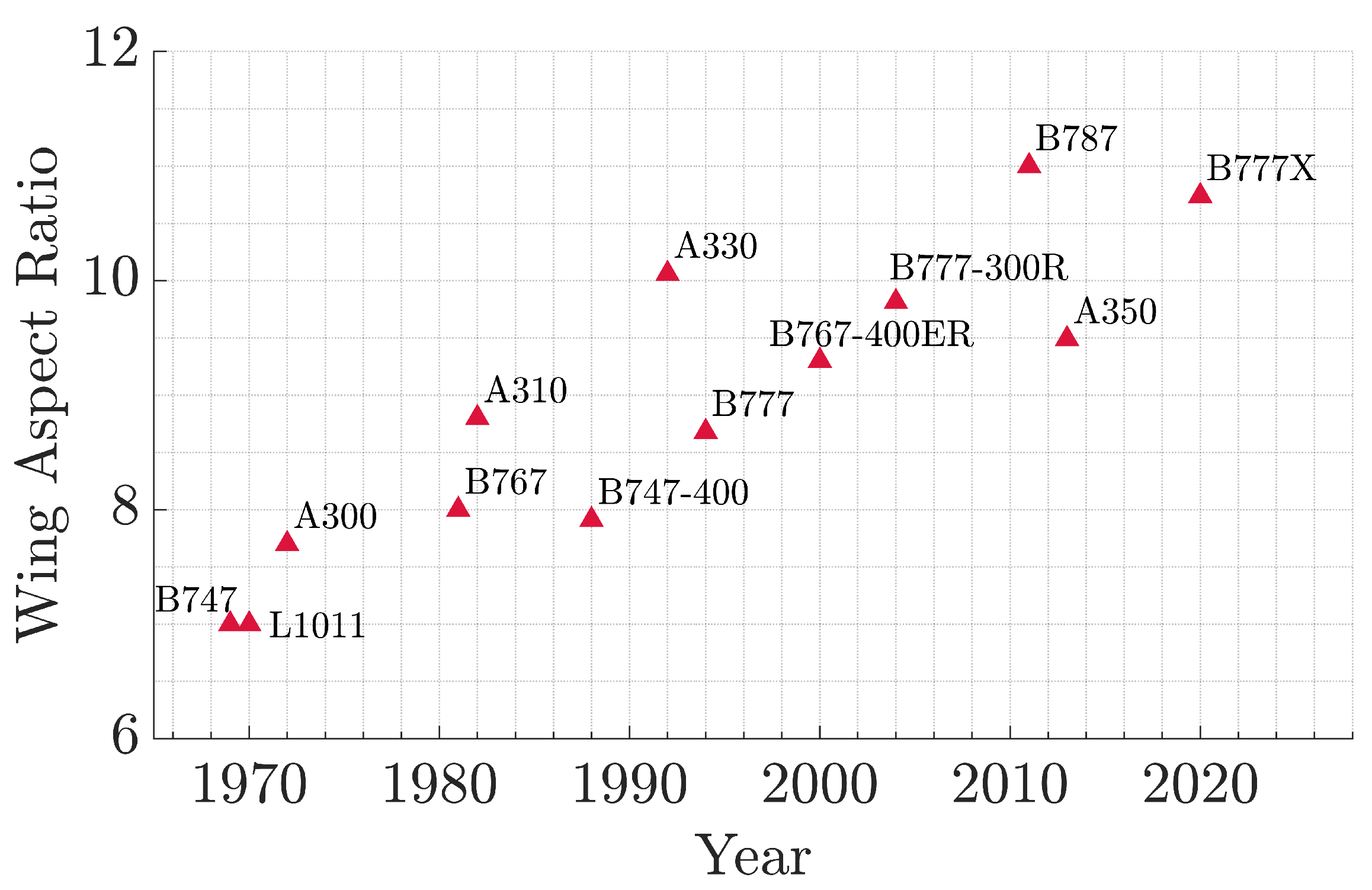
Figure 1.
Commercial aircraft wings aspect ratio trend. (Adapted from [
4]).
Figure 1.
Commercial aircraft wings aspect ratio trend. (Adapted from [
4]).
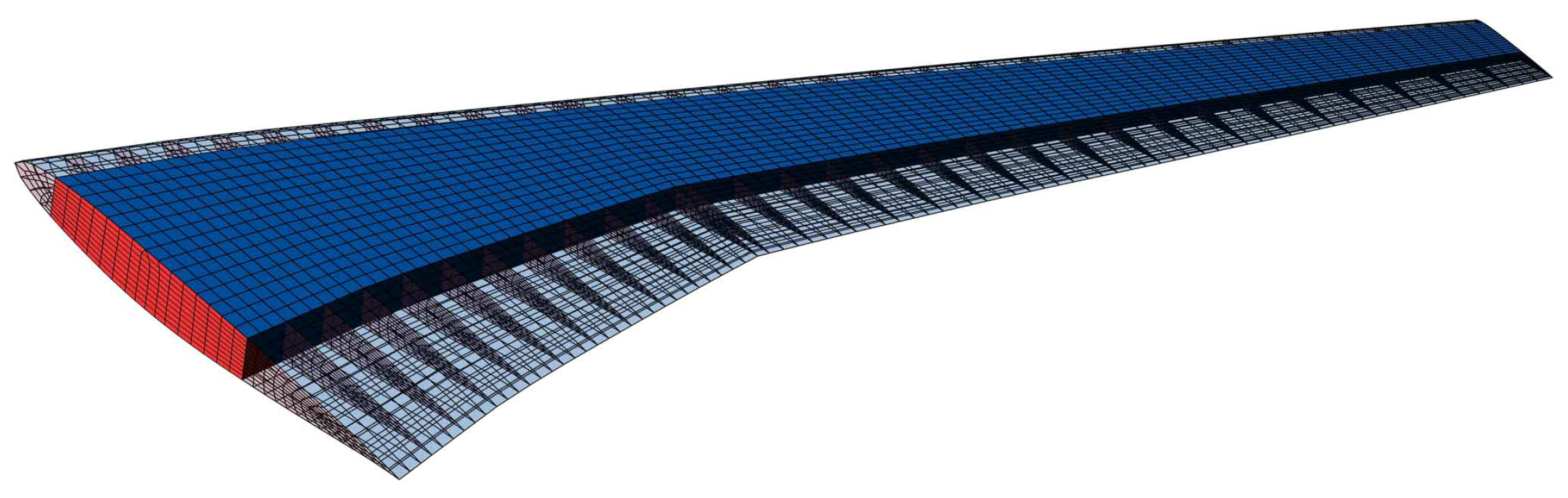
Figure 2.
Example of FEM mesh with shell and beam elements.
Figure 2.
Example of FEM mesh with shell and beam elements.
Figure 3.
3D wing surface modeled by flat panels.
Figure 3.
3D wing surface modeled by flat panels.
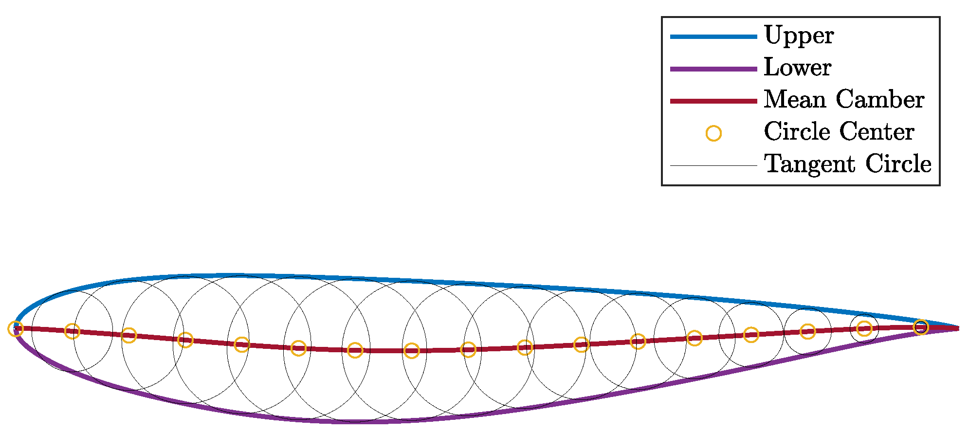
Figure 4.
Mean camber line construction method.
Figure 4.
Mean camber line construction method.
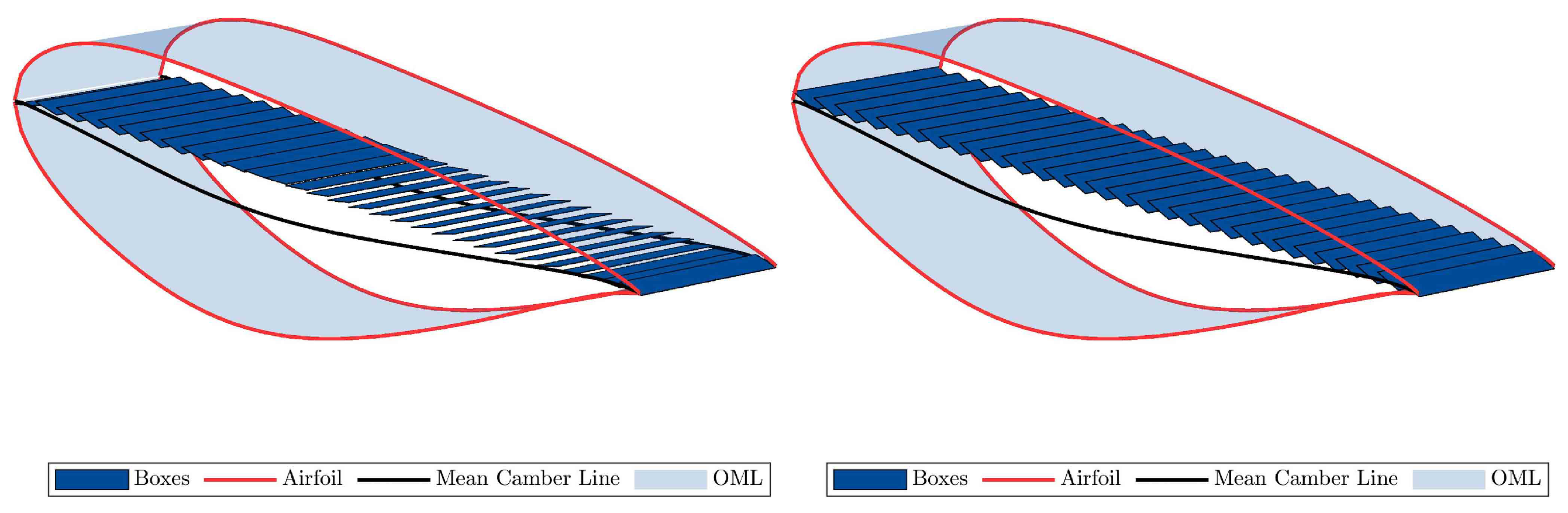
Figure 5.
W2GJ matrix influence on boxes’ inclination for camber (left) and twist (right).
Figure 5.
W2GJ matrix influence on boxes’ inclination for camber (left) and twist (right).
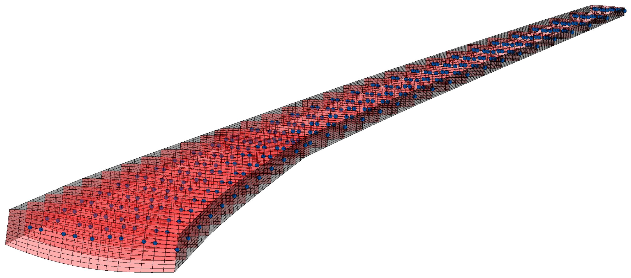
Figure 6.
Example of coupling nodes in a wing.
Figure 6.
Example of coupling nodes in a wing.
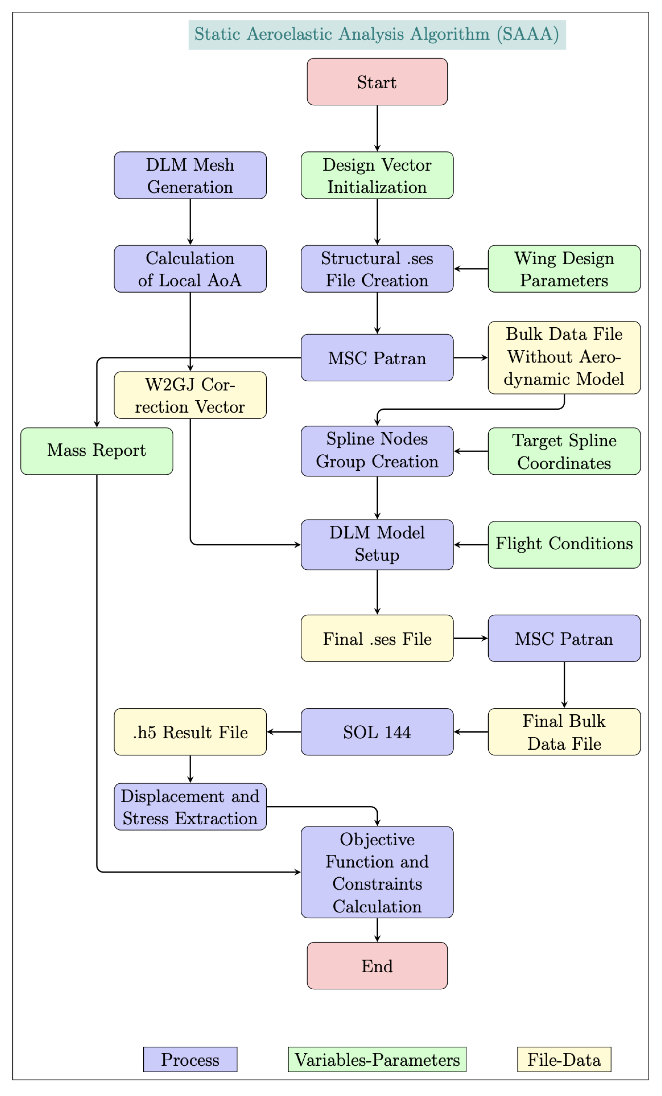
Figure 7.
Static aeroelastic framework flowchart.
Figure 7.
Static aeroelastic framework flowchart.
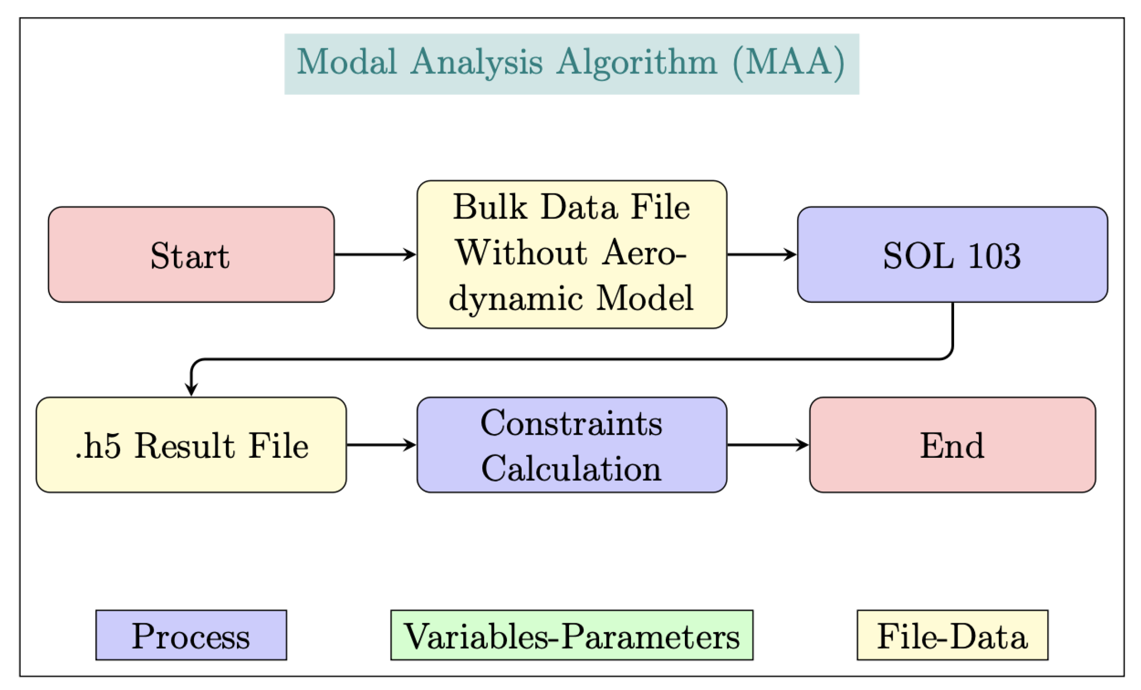
Figure 8.
Modal analysis framework flowchart.
Figure 8.
Modal analysis framework flowchart.
Figure 9.
Dynamic aeroelastic framework flowchart.
Figure 9.
Dynamic aeroelastic framework flowchart.
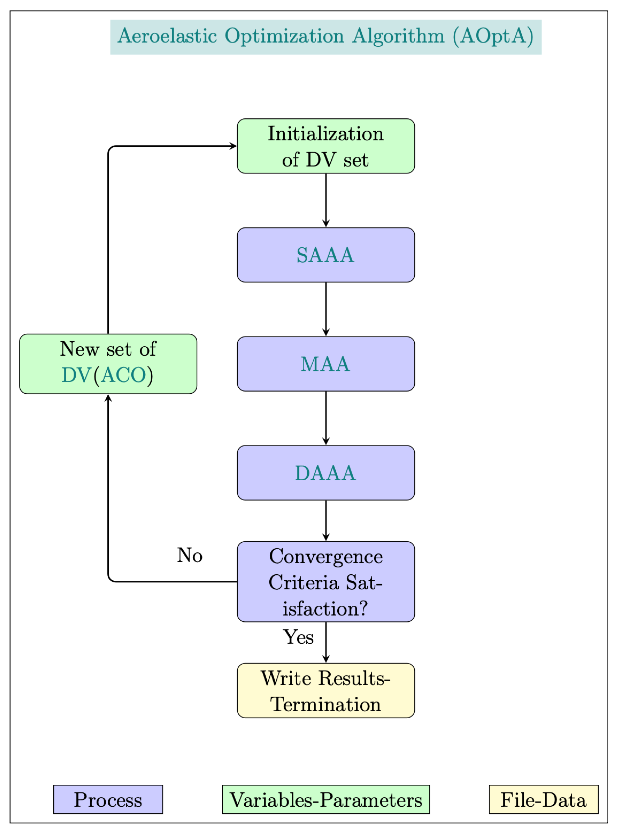
Figure 10.
Aeroelastic optimization framework flowchart.
Figure 10.
Aeroelastic optimization framework flowchart.
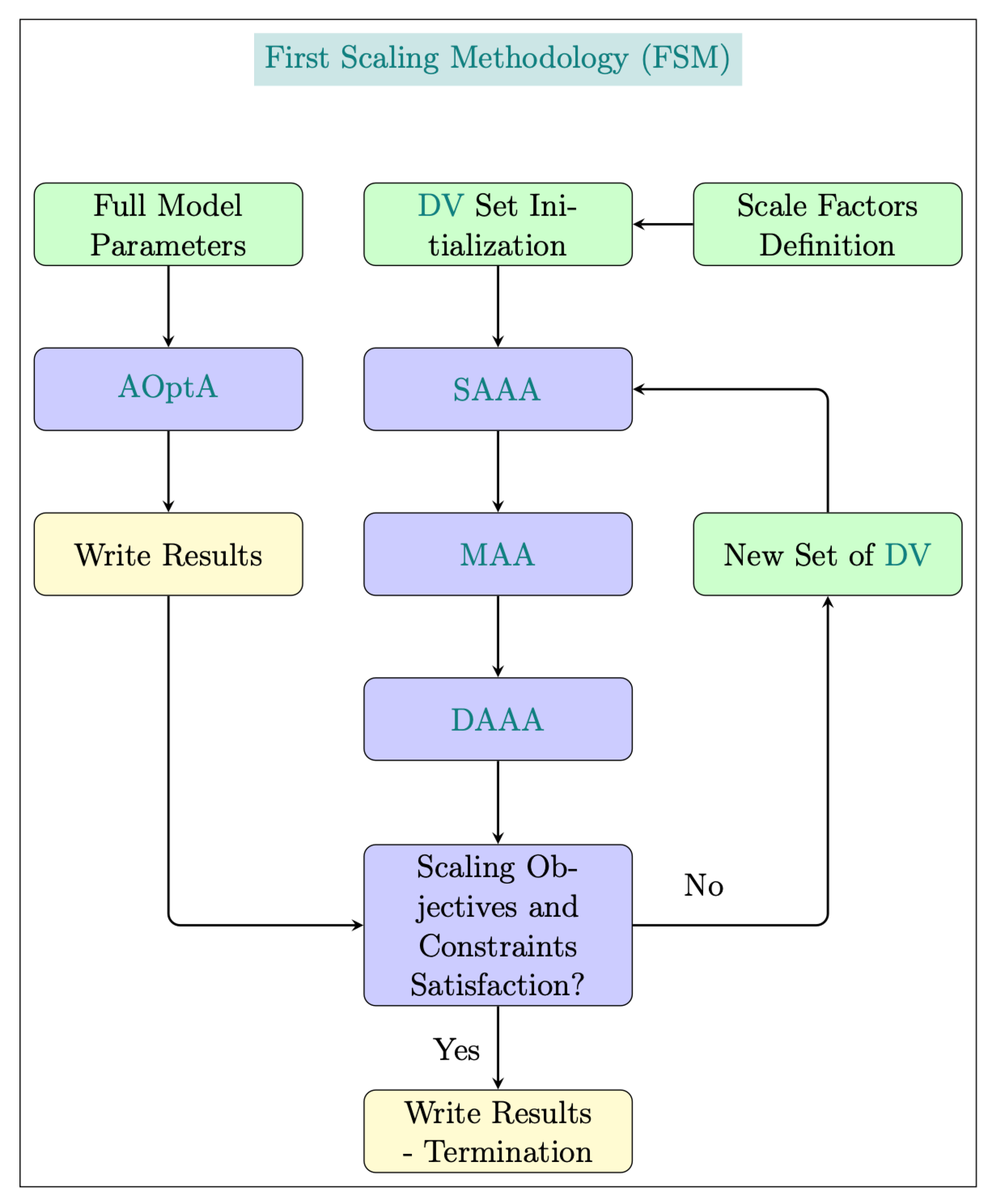
Figure 11.
Aeroelastic scaling framework flowchart.
Figure 11.
Aeroelastic scaling framework flowchart.
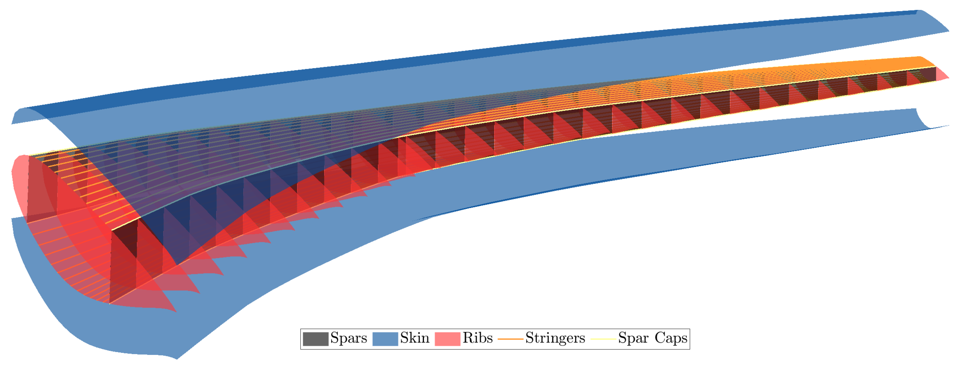
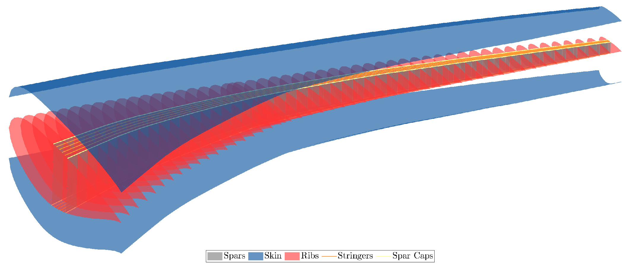
Figure 12.
uCRM wing OML and internal structure.
Figure 12.
uCRM wing OML and internal structure.
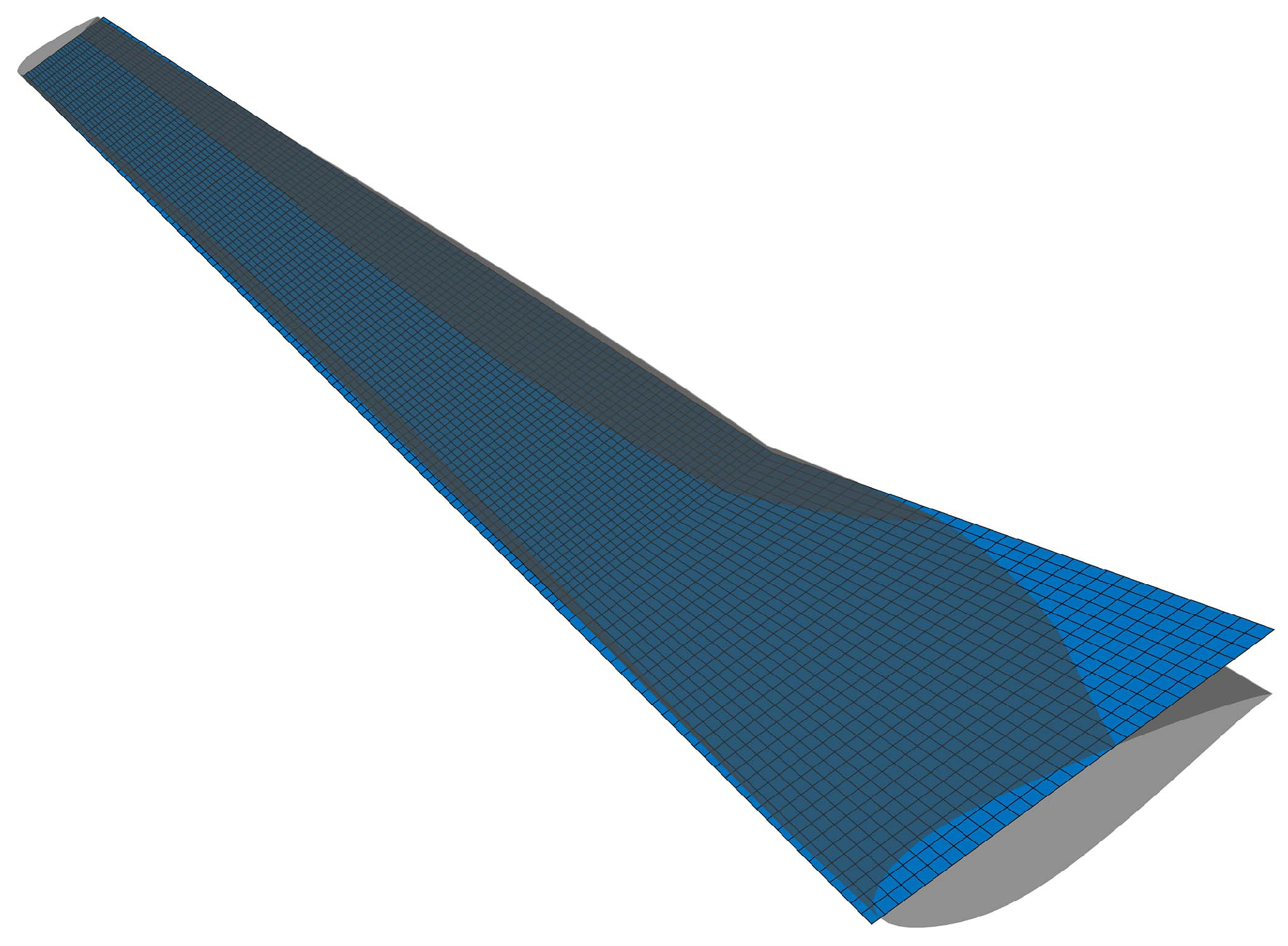
Figure 13.
3D view of the optimized geometry.
Figure 13.
3D view of the optimized geometry.
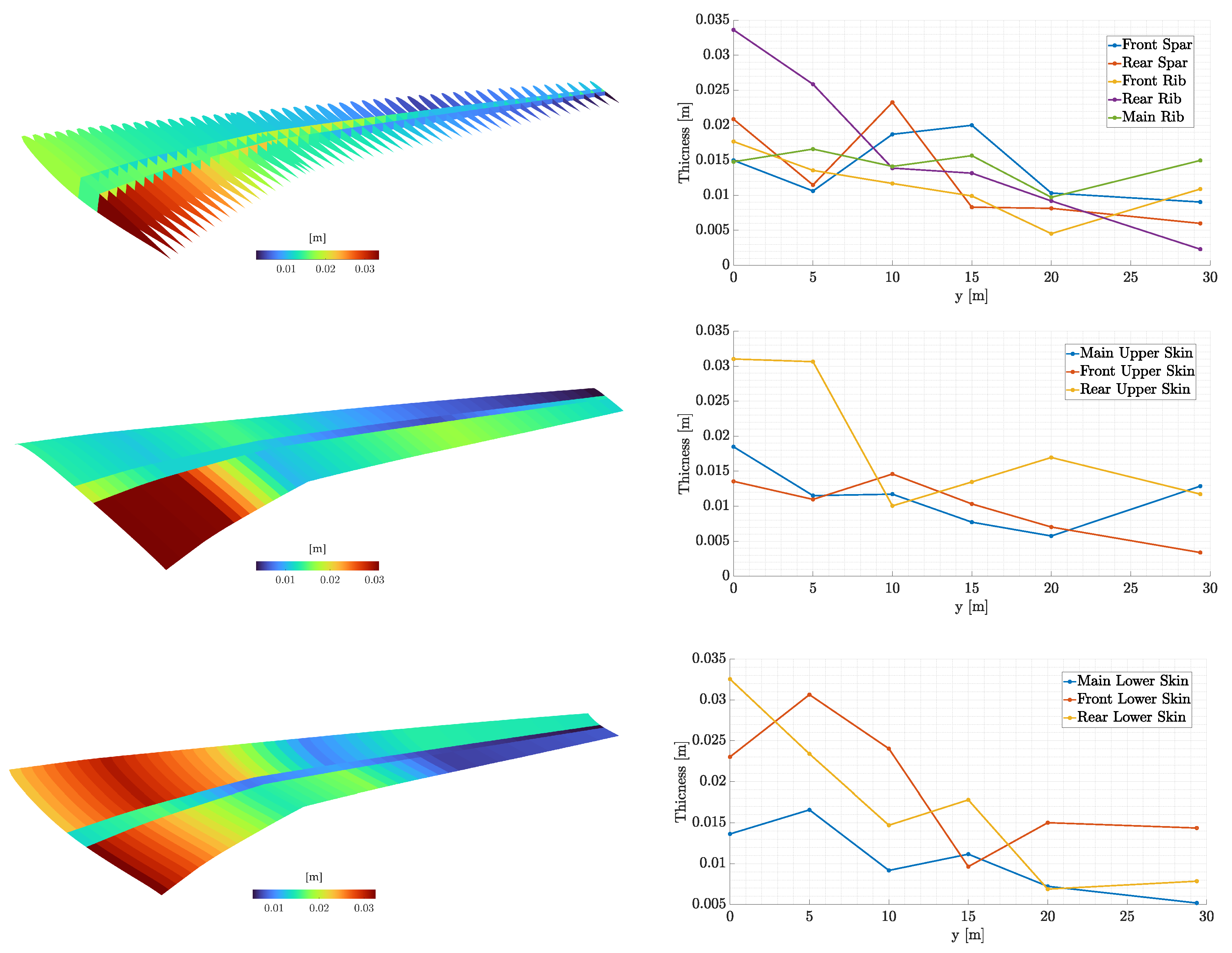
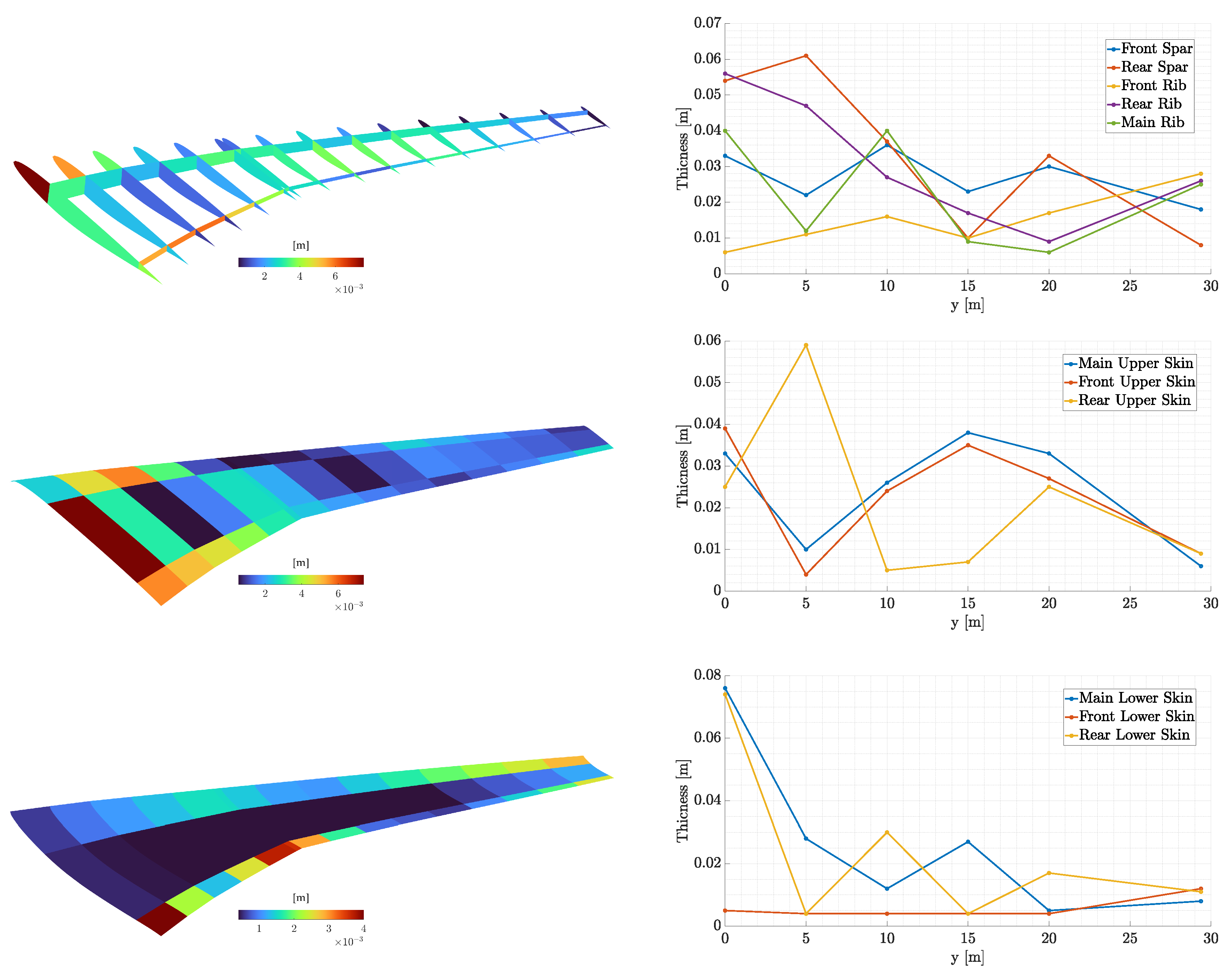
Figure 14.
Optimized thickness distribution of the internal geometry (top), upper (middle) and lower (bottom) skins along with the corresponding control point values.
Figure 14.
Optimized thickness distribution of the internal geometry (top), upper (middle) and lower (bottom) skins along with the corresponding control point values.
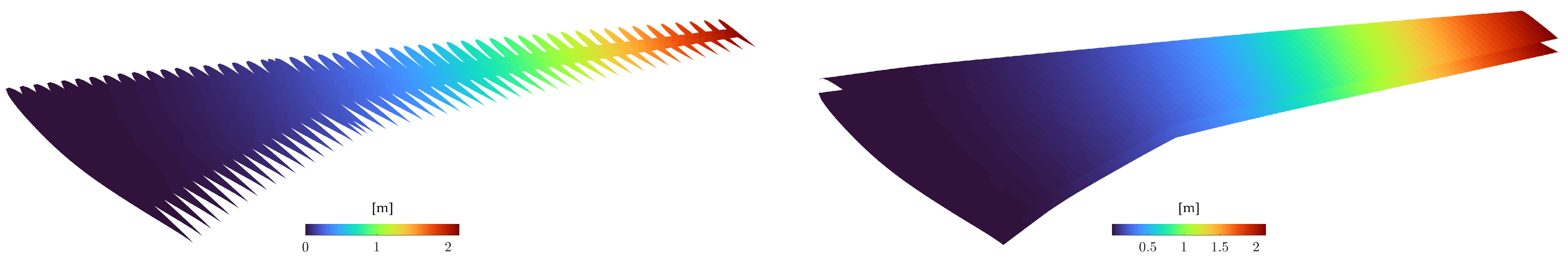
Figure 15.
Displacement distribution of the uCRM wing.
Figure 15.
Displacement distribution of the uCRM wing.
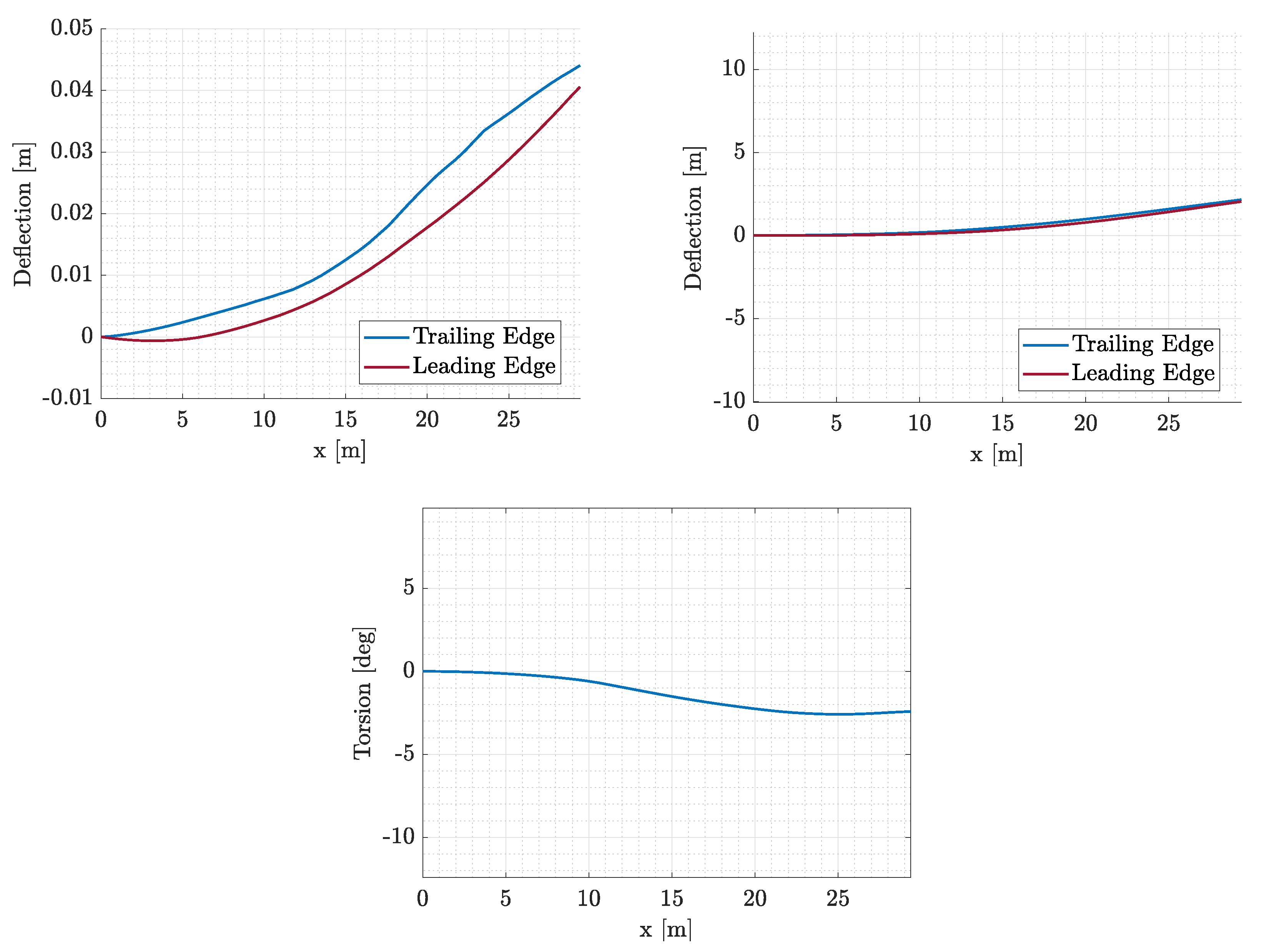
Figure 16.
Wing static aeroelastic displacements in the x (top left), z (top right) direction and torsion angle (bottom).
Figure 16.
Wing static aeroelastic displacements in the x (top left), z (top right) direction and torsion angle (bottom).
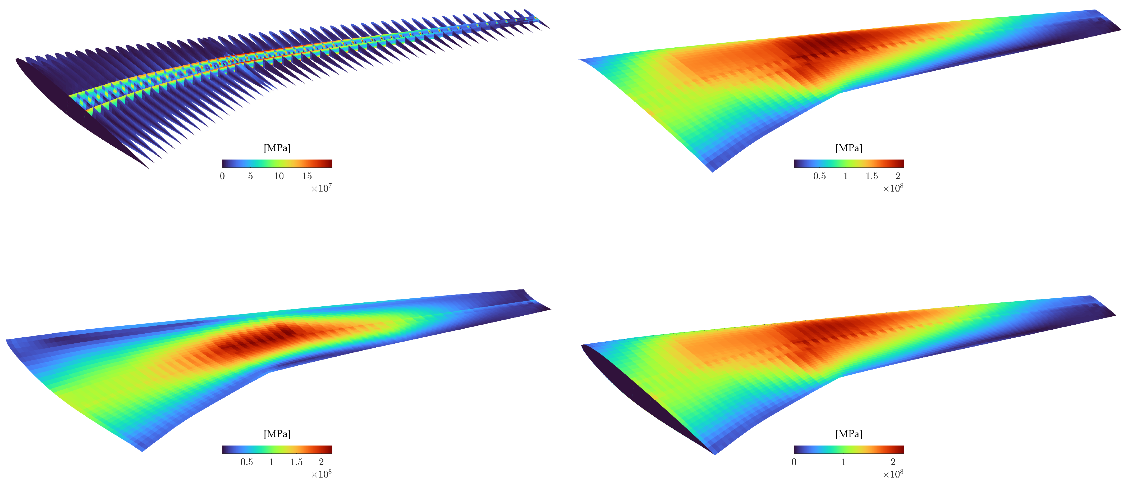
Figure 17.
Von Mises stress distribution of the uCRM wing.
Figure 17.
Von Mises stress distribution of the uCRM wing.
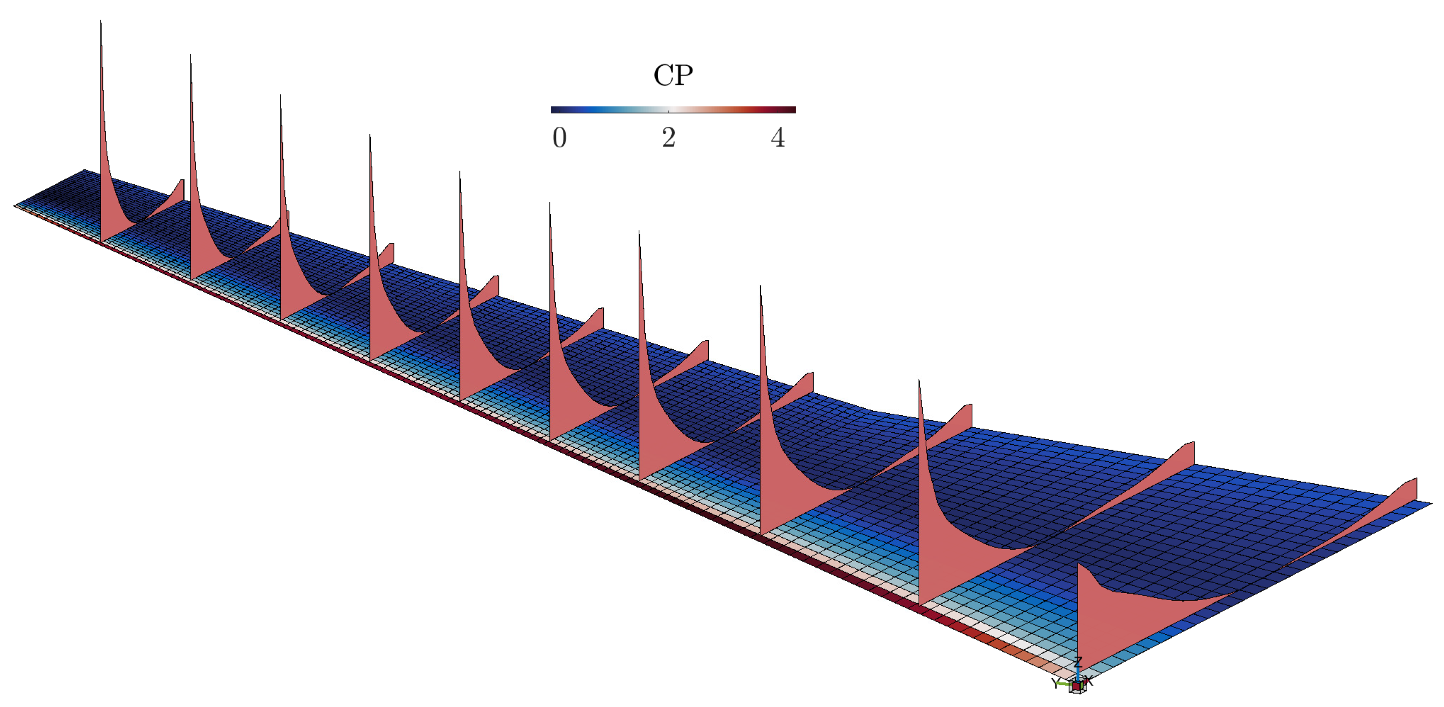
Figure 18.
Coefficient of pressure distribution.
Figure 18.
Coefficient of pressure distribution.
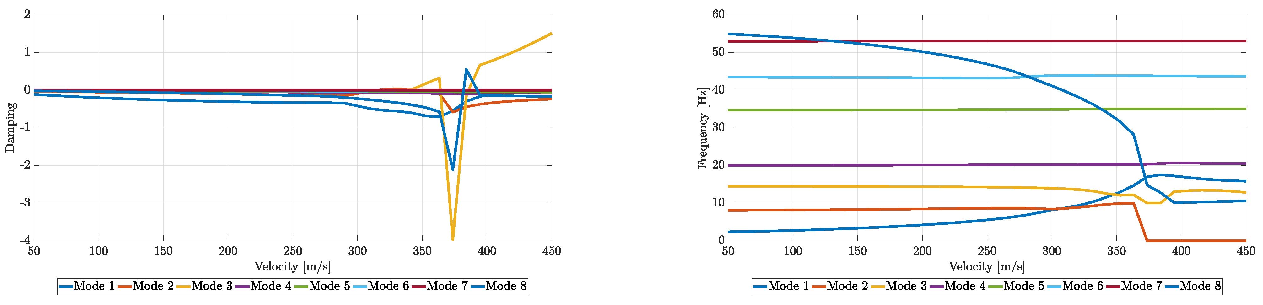
Figure 19.
V–g (left) and V–f (right) plots.
Figure 19.
V–g (left) and V–f (right) plots.
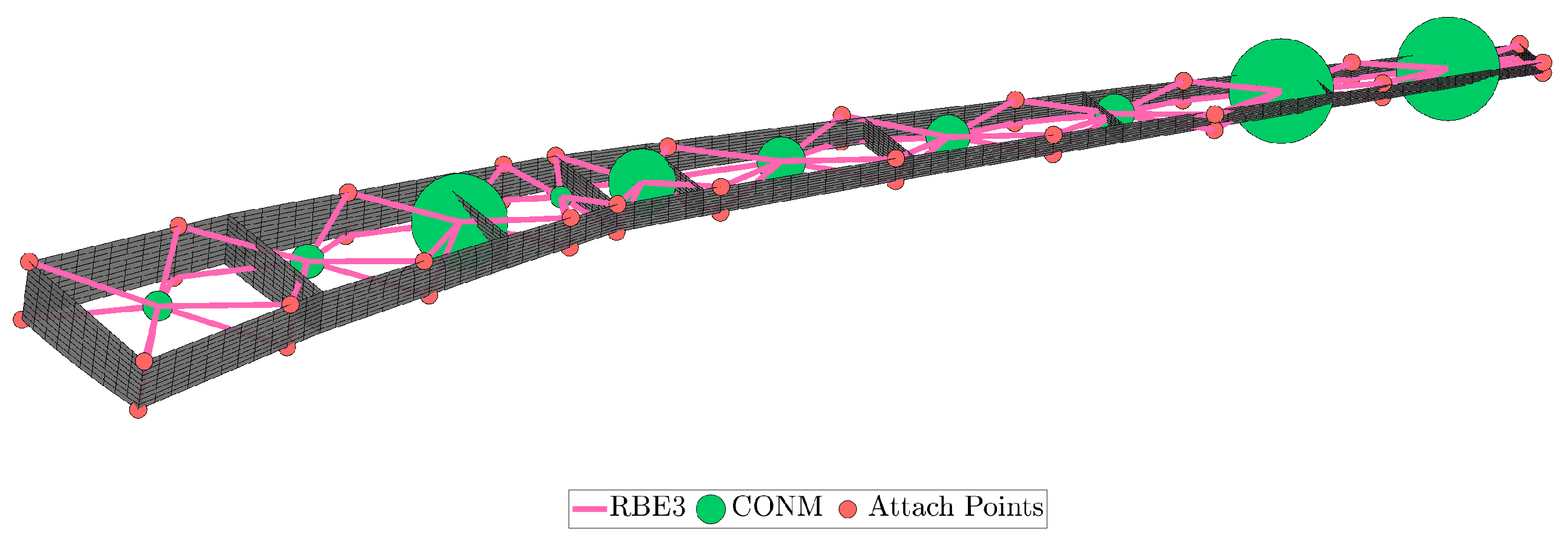
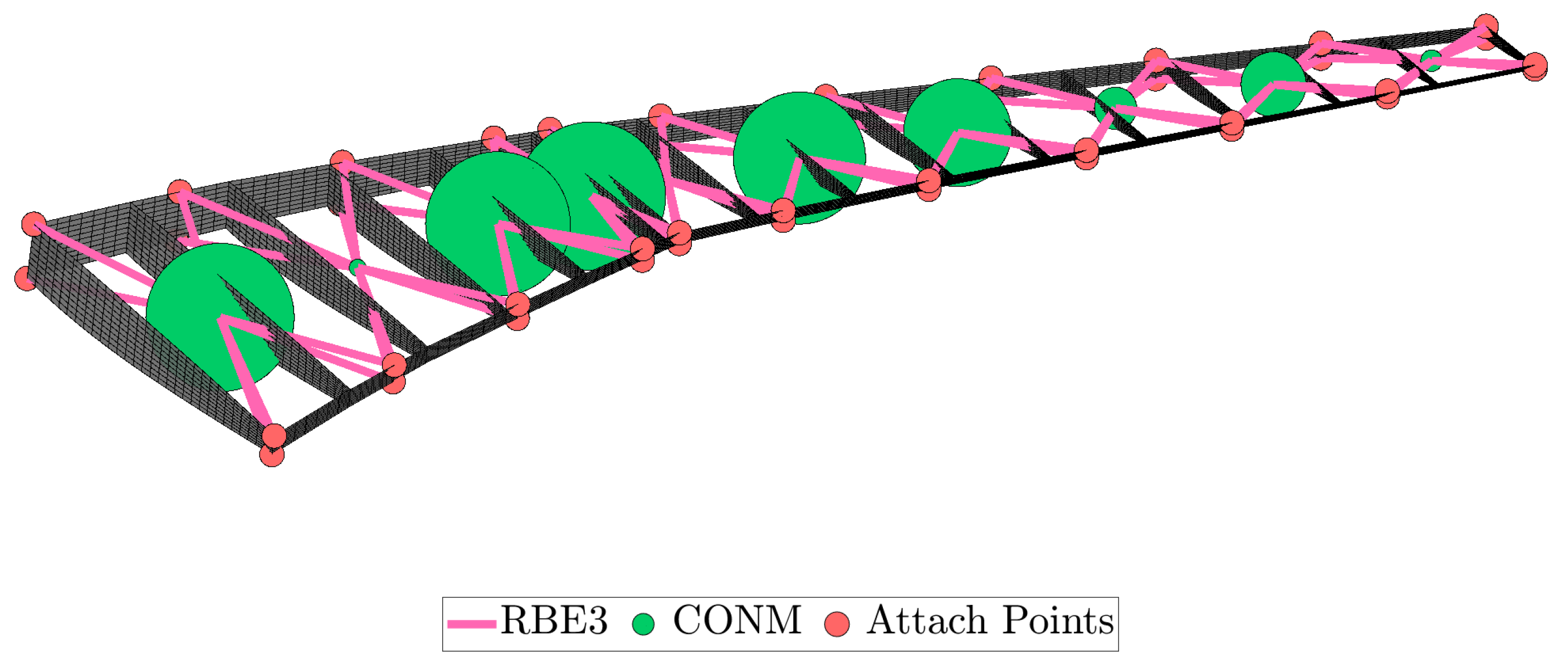
Figure 20.
Lumped masses for scaling.
Figure 20.
Lumped masses for scaling.
Figure 21.
Optimized thickness distribution of each component and its corresponding control point values for the scaling problem.
Figure 21.
Optimized thickness distribution of each component and its corresponding control point values for the scaling problem.
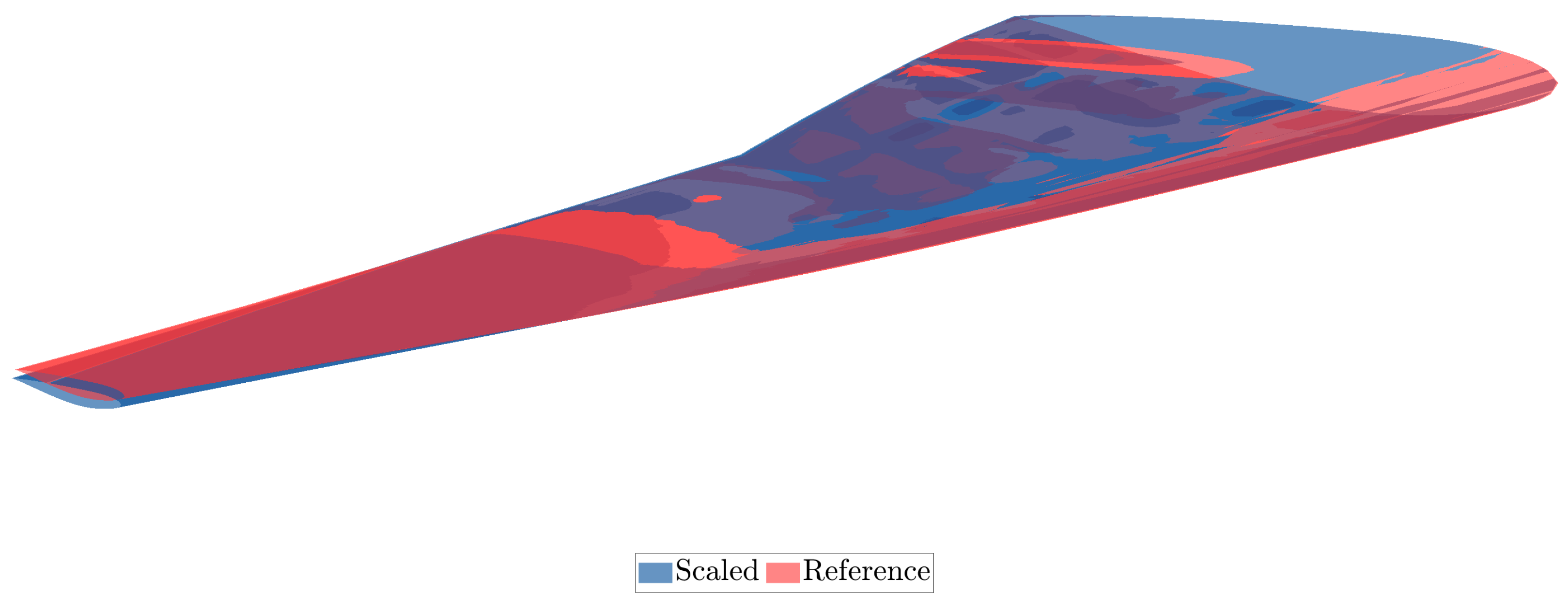
Figure 22.
In-flight aerodynamic surface of the optimized design compared to the target shape.
Figure 22.
In-flight aerodynamic surface of the optimized design compared to the target shape.
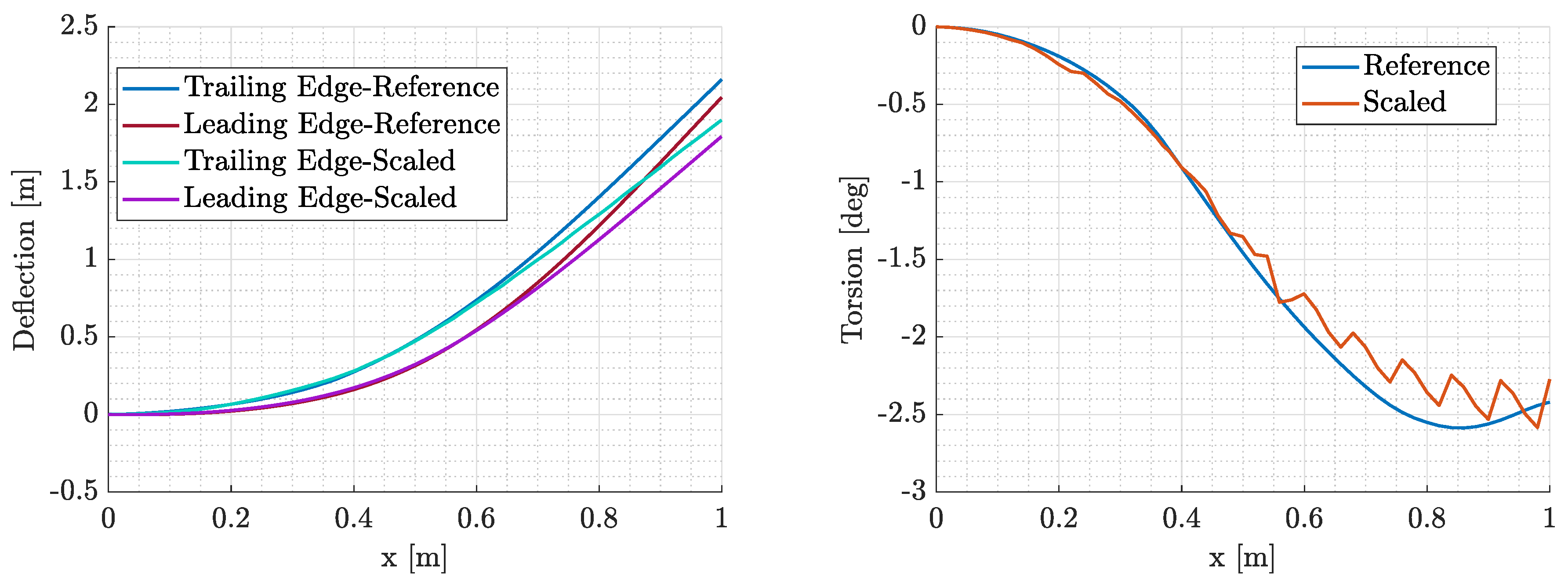
Figure 23.
Comparison of the scaled and reference wing in terms of deflection (left) and torsion angle (right).
Figure 23.
Comparison of the scaled and reference wing in terms of deflection (left) and torsion angle (right).
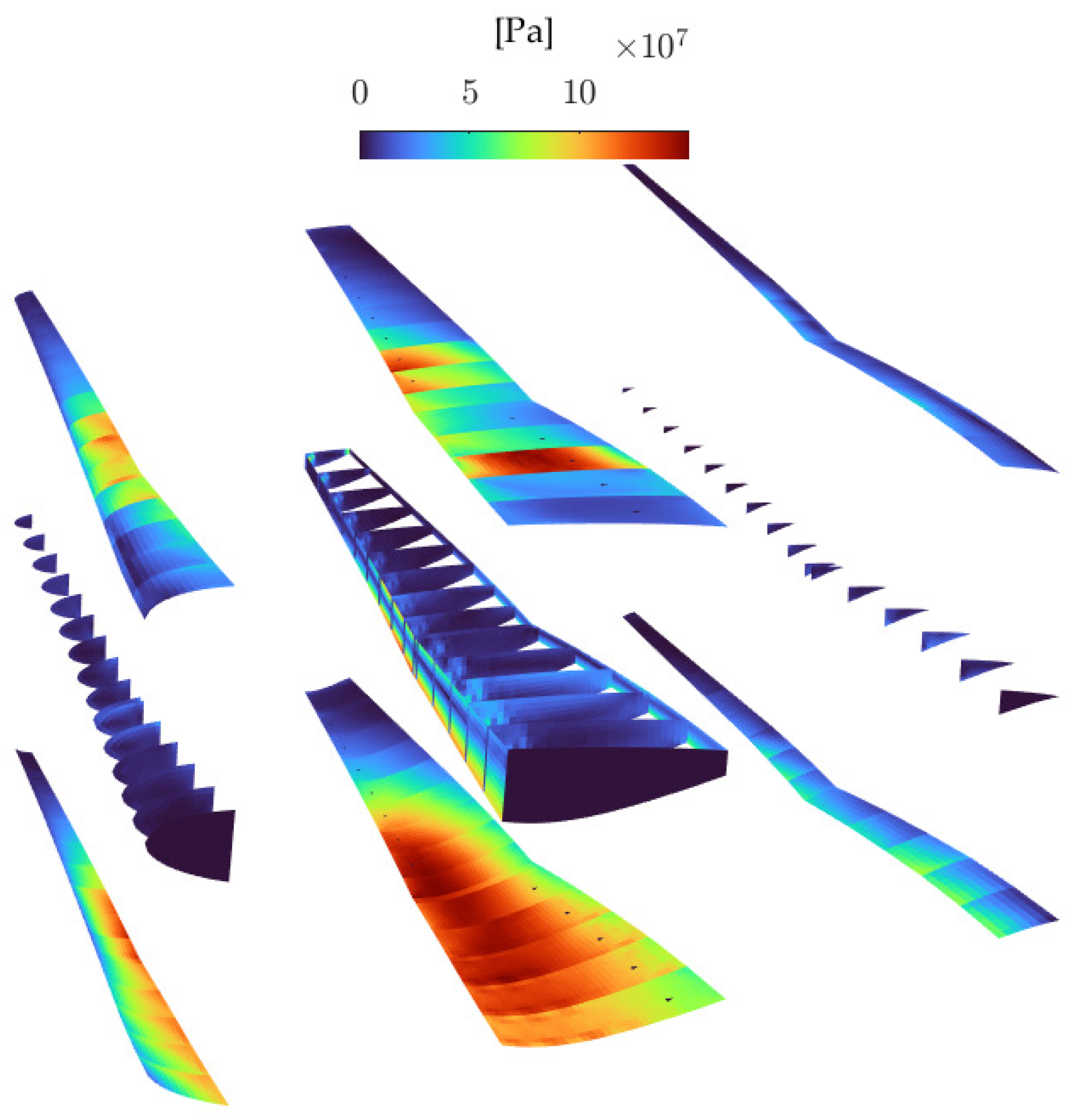
Figure 24.
Von Mises stress distribution of the scaled model.
Figure 24.
Von Mises stress distribution of the scaled model.
Figure 25.
Optimized lumped masses of the scaled model.
Figure 25.
Optimized lumped masses of the scaled model.
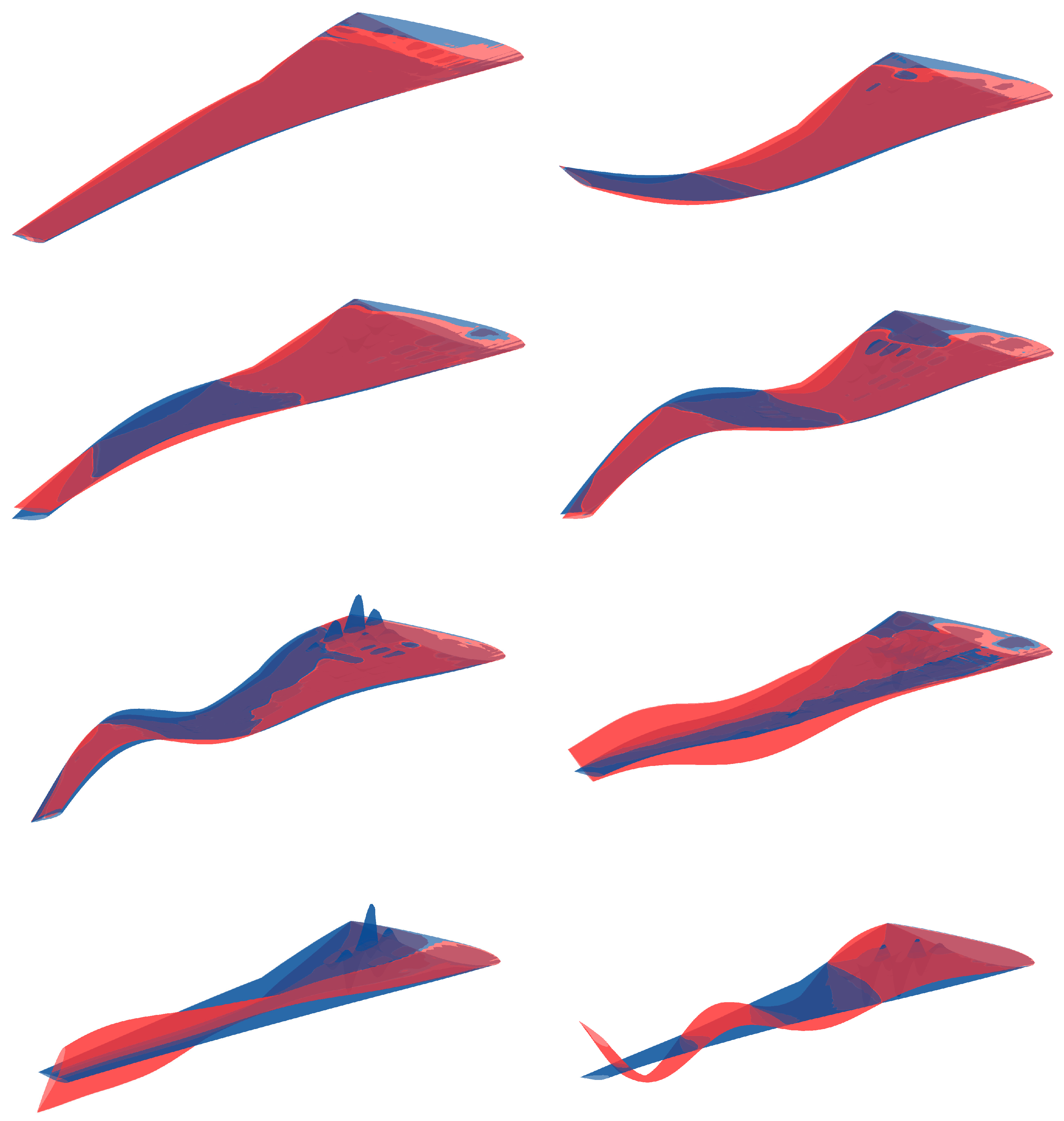
Figure 26.
First eight eigenmodes of the scaled model compared to the modes of the reference wing (red indicates undeformed shape and blue indicates the deformed shape).
Figure 26.
First eight eigenmodes of the scaled model compared to the modes of the reference wing (red indicates undeformed shape and blue indicates the deformed shape).
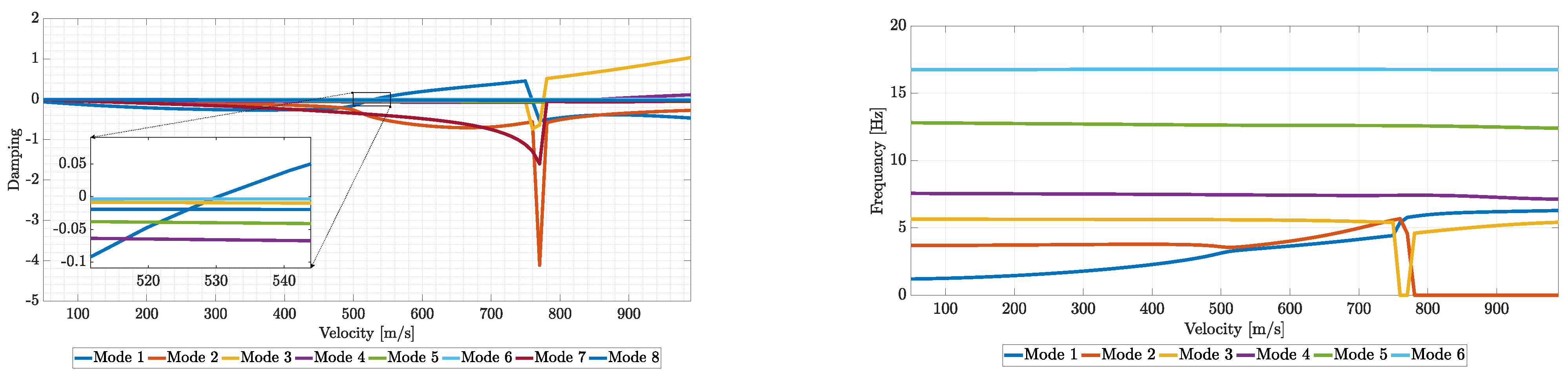
Figure 27.
V–g (left) and V–f (right) plots of the optimized scaled wing.
Figure 27.
V–g (left) and V–f (right) plots of the optimized scaled wing.
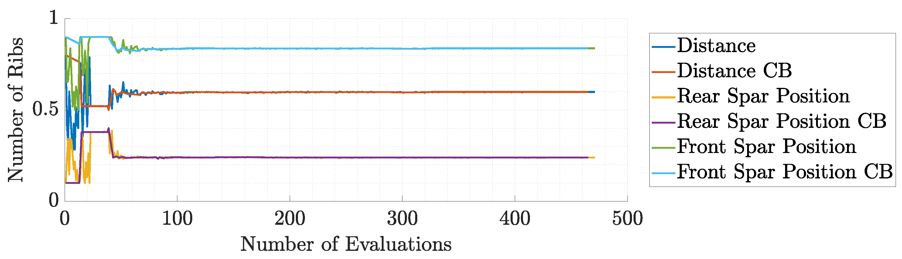
Figure 28.
Spars’ position during the 1st run of static aeroelastic response optimization.
Figure 28.
Spars’ position during the 1st run of static aeroelastic response optimization.
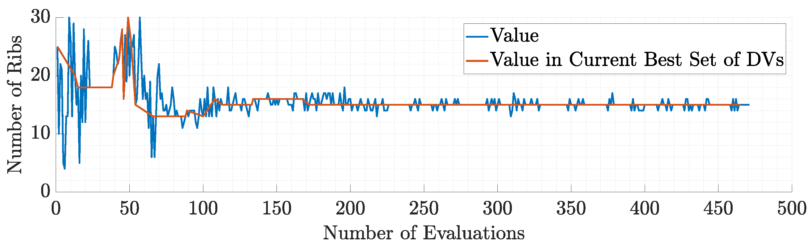
Figure 29.
Number of ribs during the 1st run of static aeroelastic response optimization.
Figure 29.
Number of ribs during the 1st run of static aeroelastic response optimization.
Table 1.
Summary of the features of the publications referenced herein (, ).
Table 1.
Summary of the features of the publications referenced herein (, ).
| Author | Aerodynamics | Structures | Optimization | Thicknesses | Topology |
|---|
| French and Eastep [9] | DLM | Beam FEM | Gradient | ✓ | ✗ |
| Richards et al. [10] | Thin Airfoil | Shell FEM | Both | ✓ | ✗ |
| Ricciardi et al. [11] | VLM | Shell FEM | Gradient | ✓ | ✗ |
| Ricciardi et al. [13] | VLM | Shell FEM | Gradient | ✓ | ✗ |
| Pontillo et al. [14] | Strip Theory | Beam FEM | Gradient | ✓ | ✗ |
| Spada et al. [15] | DLM | NL Shell FEM | Gradient | ✓ | ✗ |
| Mas Colomer et al. [19] | Panel | Shell FEM | Gradient-Free | ✓ | ✗ |
Table 2.
Aluminium’s mechanical properties.
Table 2.
Aluminium’s mechanical properties.
| Quantity | Value | Units |
|---|
| Density | 2780 | kg/m3 |
| Young’s modulus | 73.1 | GPa |
| Poisson ratio | 0.3 | - |
| Yield strength | 420 | MPa |
Table 3.
CRM geometric specifications.
Table 3.
CRM geometric specifications.
| Parameter | uCRM-9 | Units |
|---|
| Aspect Ratio | 9.0 | - |
| Span | 58.76 | m |
| Side of body chord | 11.92 | m |
| Yehudi chord | 7.26 | m |
| MAC | 7.01 | m |
| Tip chord | 2.736 | m |
| Wimpress reference area | 383.78 | m2 |
| Gross area | 412.10 | m2 |
| Exposed area | 337.05 | m2 |
| 1/4 chord sweep | 35 | deg |
| Taper ratio | 0.275 | - |
Table 4.
CRM wing critical loading conditions.
Table 4.
CRM wing critical loading conditions.
| Condition | Lift Constraint | Mach Number | Altitude (m) |
|---|
| Maneuver | 2.5 MTOW | 0.64 | 0 |
Table 5.
Objectives and constraints of the mass minimization problem.
Table 5.
Objectives and constraints of the mass minimization problem.
| Objective | Target |
|---|
| Mass | Minimization |
| under the constraints |
| Maximum Deflection | ≤ |
| Tip Torsion Angle | ≤6 deg |
| First Eigenfrequency | ≥1 Hz |
| Maximum Von Mises Stress | ≤280 MPa |
| Flutter Speed | ≥ |
Table 6.
Design variables of the optimization problem.
Table 6.
Design variables of the optimization problem.
| Variable | Lower Bound | Upper Bound | Dimension |
|---|
| Ribs Number | 6 | 52 | 1 |
| Stringers Number | 4 | 12 | 1 |
| Front Spar Position | 0.1 | 0.4 | 1 |
| Rear Spar Position | 0.5 | 0.9 | 1 |
| Stringer and Spar Cap Thickness | 1 mm | 10 mm | 2 mm |
| Thicknesses at Control Points | 2 mm | 40 mm | 66 mm |
Table 7.
MIDACO parameters.
Table 7.
MIDACO parameters.
| Run | Iterations | Accuracy | FOCUS | Initial Point |
|---|
| 1 | 250 | 0.1 | 0 | Random |
| 2 | 100 | 0.01 | 10 | Run 1 |
Table 8.
Optimization results summary.
Table 8.
Optimization results summary.
| Property | Value |
|---|
| Mass | 6902 kg |
| Minimum Eigenfrequency | 1.1735 Hz |
| Maximum Von Mises Stress | 247.5 MPa |
| Tip Torsion | 2.7 deg |
| Maximum Deflection | 7.89% of span or 2.32 m |
| Flutter Speed | 501 m/s |
Table 9.
Optimized geometric design variables.
Table 9.
Optimized geometric design variables.
| Variable | Value |
|---|
| Ribs Number | 51 |
| Stringers Number | 4 |
| Front Spar Position | 0.3904 |
| Rear Spar Position | 0.5166 |
| Stringer Thickness | 2 mm |
| Spar Cap Thickness | 3 mm |
Table 10.
Objectives and constraints of the scaling problem.
Table 10.
Objectives and constraints of the scaling problem.
| Objective | Target |
|---|
| In-Flight Shape Difference | Minimization |
| Modal Similarity (MAC) | Maximization |
Table 11.
Objectives and constraints of the mass minimization problem.
Table 11.
Objectives and constraints of the mass minimization problem.
| Constraint | Target |
|---|
| Frequency Difference | =0 Hz |
| Overall Mass | kg |
| Maximum Von Mises Stress | ≤280 MPa |
Table 12.
Target values of frequency for the optimization problem.
Table 12.
Target values of frequency for the optimization problem.
| Mode Number | Reference Wing Frequency, Hz | Scaled Wing Frequency, Hz |
|---|
| 1 | 1.1915 | 2.6642 |
| 2 | 3.7067 | 8.2885 |
| 3 | 5.6416 | 12.6151 |
| 4th | 7.58 Hz | 16.9494 |
| 5th | 12.8288 | 28.6861 |
| 6th | 16.7503 | 37.4548 |
| 7th | 17.9140 | 40.0570 |
| 8th | 19.4901 | 43.5812 |
Table 13.
Design variables of the optimization problem.
Table 13.
Design variables of the optimization problem.
| Variable | Lower Bound | Upper Bound | Dimension |
|---|
| Ribs Number | 6 | 30 | 1 |
| Stringers Number | 4 | 10 | 1 |
| Front Spar Position | 0.1 | 0.4 | 1 |
| Rear Spar Position | 0.5 | 0.9 | 1 |
| Thicknesses at Control Points | 0.4 mm | 8 mm | 66 |
| Lumped Masses | 100 mg | 60 kg | 10 |
Table 14.
Magnesium’s mechanical properties.
Table 14.
Magnesium’s mechanical properties.
| Quantity | Value | Units |
|---|
| Density | 1800 | kg/m3 |
| Young’s modulus | 45 | GPa |
| Poisson ratio | 0.35 | - |
| Yield strength | 150 | MPa |
Table 15.
MIDACO parameters of the static aeroelastic response similarity optimization.
Table 15.
MIDACO parameters of the static aeroelastic response similarity optimization.
| Run | Iterations | Accuracy | FOCUS | Initial Point |
|---|
| 1 | 500 | 0.1 | 0 | Random |
| 2 | 100 | 0.01 | 10 | Run 1 |
Table 16.
Optimized geometric design variables.
Table 16.
Optimized geometric design variables.
| Variable | Value |
|---|
| Ribs Number | 15 |
| Stringers Number | 5 |
| Front Spar Position | 0.239 |
| Rear Spar Position | 0.839 |
Table 17.
Optimized mass values for the modal response similarity optimization problem.
Table 17.
Optimized mass values for the modal response similarity optimization problem.
| Mass | Value [kg] |
|---|
| 1 | 79.78 |
| 2 | 9.13 |
| 3 | 77.79 |
| 4 | 79.86 |
| 5 | 0.01 |
| 6 | 71.07 |
| 7 | 58.12 |
| 8 | 22.79 |
| 9 | 35.20 |
| 10 | 11.64 |
Table 18.
Target values of frequency for the optimization problem.
Table 18.
Target values of frequency for the optimization problem.
| Mode Number | Target | Optimized | Error |
|---|
| 1 | 2.6642 Hz | 2.2743 Hz | 14.63% |
| 2 | 8.2885 Hz | 8.0904 Hz | 2.39% |
| 3 | 12.6151 Hz | 14.4570 Hz | 14.60% |
| 4 | 16.9494 Hz | 20.1439 Hz | 18.84% |
| 5 | 28.6861 Hz | 34.9225 Hz | 21.76% |
Table 19.
Effectiveness of the proposed aeroelastic scaling framework.
Table 19.
Effectiveness of the proposed aeroelastic scaling framework.
| Run | Description | MAC | Deviation, % |
|---|
| 1 | Proposed Framework | 0.93 | - |
| 2 | Number of Ribs = 5 | 0.67 | 27.9 |
| 3 | Number of Ribs = 30 | 0.59 | 36.5 |
| 4 | Number of Ribs = 30, Spars Positions Fixed | 0.72 | 22 |


 ,
, 


