Modelling of Cryopumps for Space Electric Propulsion Usage

Abstract

Electric space propulsion is a technology that is used in a continuously increasing number of spacecrafts. The qualification of these propulsion systems has to run in ground-based test facilities which requires long testing times and powerful pumping systems. In these usually large test facilities, high pumping speeds are achieved with cryopumps. Cryopump operation is very expensive with respect to electrical energy and cooling water consumption. Therefore, being able to optimize pump shape, cold plate material, and pump placement in a chamber is beneficial. Pump design and tuned operating strategies can reduce costs and increase intervals between regeneration. Testing different pump configuration setups in a large facility is mostly prohibitive due to high costs and long testing times. Optimization via modelling is a better choice for design and also, later, for operation. Therefore, having a numerical model and proven guidelines at hand for optimization is very helpful. This paper describes a new model developed at DLR for the optimization of cryopump layout and operation. Model results are compared with cryopump operational and warm-up data. This validation is the basis for further optimization actions like multi-layer insulation layouts and pump cold plate upgrades, and helps in understanding and mitigating the detrimental effect of water condensates on the cryopump cold plates.

1. Introduction

Electric propulsion is currently used routinely for satellite station keeping, and R&D developments and qualification are pointing towards full electric orbit transfer [1]. Electric propulsion is also gaining more interest in the sector as future science missions request very low thrust in conjunction with low thrust noise and accurate thrust level control [1,2,3]. Today, the satellite onboard electrical power is of the order of several kW for a somewhat larger telecom satellite. With this, the maximum EP thrust is in the range of a fraction of a Newton, based on a thrust to power ratio of 40–70 mN/kW [2,3]. Mission requirements like orbit raising or maneuvering therefore require longer accumulated thruster runtimes of many days or months. These runtimes lead to EP qualification on-ground test programs lasting thousands of hours, and vacuum facilities have to run reliably for these long times [4]. This includes powerful pumping systems, mostly equipped with cryopumps that freeze propellant gases on cold surfaces and are able to reach very high pumping speeds. Therefore, cryopumps are a crucial part of large EP test facilities.

2. DLR Electric Propulsion Test Facility Göttingen

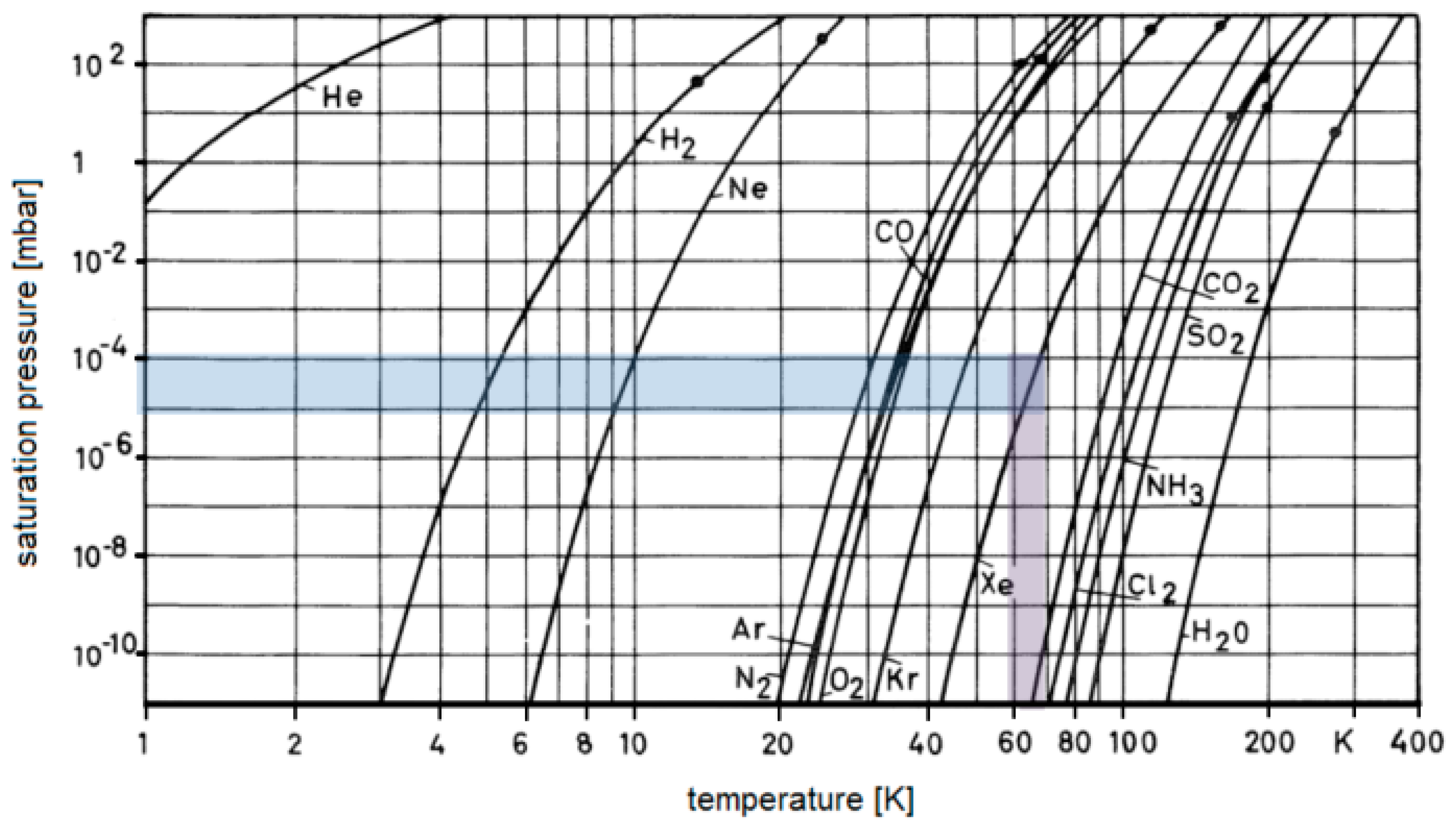
Since 2011, DLR has operated an electric space propulsion test facility, the STG-ET (Simulationsanlage Treibstahlen Göttingen—Elektrische Triebwerke). A central element of this facility is a 12.2 m long and 5 m diameter vacuum chamber (Figure 1) [5]. The chamber is mounted on sliding bearings which reduce mechanical stresses in case of pump-down and temperature changes. The device under test and main diagnostics equipment are positioned on a 2.5 m high stand which is decoupled from the metal chamber wall and directly connected to the concrete foundation of the building. This decoupling ensures less vibration for accurate thrust measurement, and a stable and well-defined space coordinate system.

Rough pumping is achieved by a rotating vane plus a Roots pump stand, and high vacuum is achieved via four turbo pumps. The operation of thrusters with a high gas mass flow requires a high pumping speed, and, in this case, up to 18 cryopumps can be activated. With this arrangement, it is possible to reach a standby background pressure of around 10⁻⁷ mbar. The required vacuum chamber pressure during thruster operation is usually around 10⁻⁵–10⁻⁴ mbar, which is a typical requirement for EP thrusters [6,7,8]. This range is also confirmed by our test campaigns, performed over the last decade [9].

EP thrusters and especially ion thrusters generate beams of fast ions that interact with the facility walls and equipment. These high velocity ions cause sputtering when hitting the walls of the chamber or all other components located inside the chamber. In general, facility contaminating and other unwanted sputtering effects occur with all typical electric space propulsion systems, and mainly, in ground test chambers for long term qualification, dedicated beam dump targets are used for the reduction of sputtering effects. The STG-ET has two beam dump targets, one at the chamber end consisting of water-cooled stainless-steel plates coated with graphite sheets, and similar graphite sheets protect part of the chamber cylinder mantle (Figure 1). These graphite liners have a low sputtering coefficient compared with stainless steel (section on ion thruster grids in [10,11,12,13]).

3. Cryopump Basics

The pumping systems of a ground-based facility must be able to cope with thruster gas flow, which is of the order of 5–20 mg/s for a typical thruster of 5 kW, depending on the thruster technology (Hall effect [6], RIT, other gridded ion thruster, or others [7]).

Currently, xenon is the preferred propellant for the mentioned thrusters. Under high vacuum conditions with molecular flow, pumping speed scales with pump aperture area and the preferred way of trapping gas is to use cryo-trapping on cold surfaces. The pumping speed for xenon is of the order of a few l·s⁻¹ cm⁻² for cryopumps, which is similar to turbo molecular pumps [14]. Normally, it is much simpler to install a large cold surface plate of m² size, instead of having a large 1 m² entry area turbo pump with fast rotating components. This explains why cryopumps are usually the preferred method if high gas loads are present. Commercially available cryopumps come in different configurations [14]. The standard type has a two-stage head contained in a vessel of standard diameters (e.g., up to 500 mm) which is equipped with baffles. These pumps are meant primarily for processes under high vacuum and air pumping (oxygen, nitrogen), e.g., material processing, particle physics, etc. The pumping speed of such a design is much lower for xenon than for air.

For EP applications that use thrusters with a gas throughput running in a vacuum using xenon as propellant, single-stage open cryopanel pumps are one option that may also be more economic than baffled one- or two-stage pumps [13]. In the open configuration, a copper plate (sometimes nickel-plated) is directly attached to the cold head, and this assembly protrudes into the vacuum chamber without housing or baffles, as can be seen in Figure 1. The use of open single-stage cryopumps is also in the portfolio of manufacturers, e.g., [14]. If the plate temperature is below 55–60 K in the typical EP operating pressure range of 10⁻⁴–10⁻⁵ mbar, see phase diagram in Figure 2, xenon freezes and the pumping process takes place. It should be noted that if the plate temperature stays above approximately 35 K, the cryopump will not pump air constituents (oxygen, nitrogen, argon, see Figure 2).

Another advantage of single cryopump plates without baffles or shrouds is the easier cleaning process. Electric space propulsion long duration tests produce a lot of sputter debris in the chamber. This sputtered material is deposited everywhere in the chamber, and removing it is work intensive. Therefore, single-plate open pumps are much easier to clean.

A general issue for cryopumping is water, as this starts to freeze at temperatures below 200 K. This is especially true when using the open single-stage design. Baffles are often cooled with liquid nitrogen (LN2) and act as condensation surfaces for water. This partly protects the cryopump cold plates from water ice [14,15,16]. The issue with water ice on open cold plates is the following. The absorption of thermal radiation on pump cold plates, e.g., from chamber walls, is governed by the emissivity ε. For water condensate (ice), its emissivity is high compared with xenon, around 0.8–0.95 (see Section 7.3). As a consequence, the heat load on a pumping surface covered with a water ice layer is very high and deteriorates the pump performance causing a faster warm-up.

Figure 2. Saturation pressures of several gases important to vacuum technology and electric space propulsion. The shaded area highlights xenon (adapted from [16]). The shades parts show the pressure and temperature operation ranges for xenon in thruster application.

Figure 2. Saturation pressures of several gases important to vacuum technology and electric space propulsion. The shaded area highlights xenon (adapted from [16]). The shades parts show the pressure and temperature operation ranges for xenon in thruster application.

When designing the DLR vacuum facility, we originally planned the pumping system based on baffled cryopumps. But after reviewing the issues with mounting, cleaning, LN2-cooled baffles, more complex process controls, and potentially more leaking points, the baffled design was abandoned (Figure 1).

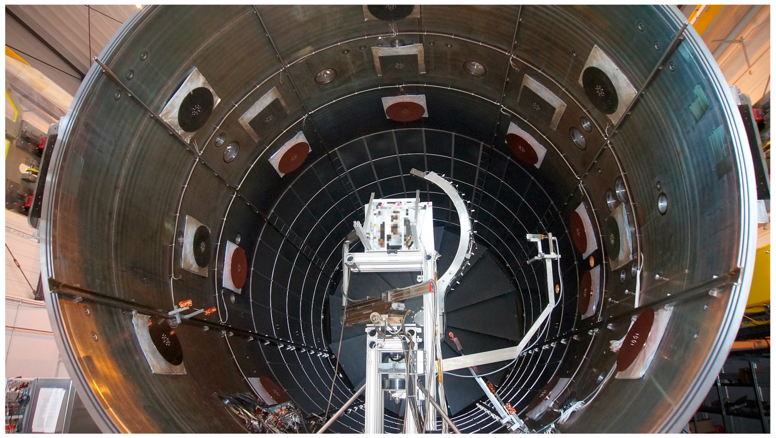
4. DLR STG-ET Pumping System

Figure 3 shows a schematic of the pumping system in DLR’s facility. A dedicated roughing pump system (rotating vane and Roots pump 2), directly attached to the vacuum chamber, generates the necessary vacuum level for a switch-on of the turbomolecular pumps, which have their own backing pump stand. Under thruster operation, up to 18 cryogenic pumps remove the propellant gas [10,17].

Since the cryopumps were installed at different times and in three lots, they have differently sized cold plates. The actual configuration is as follows:

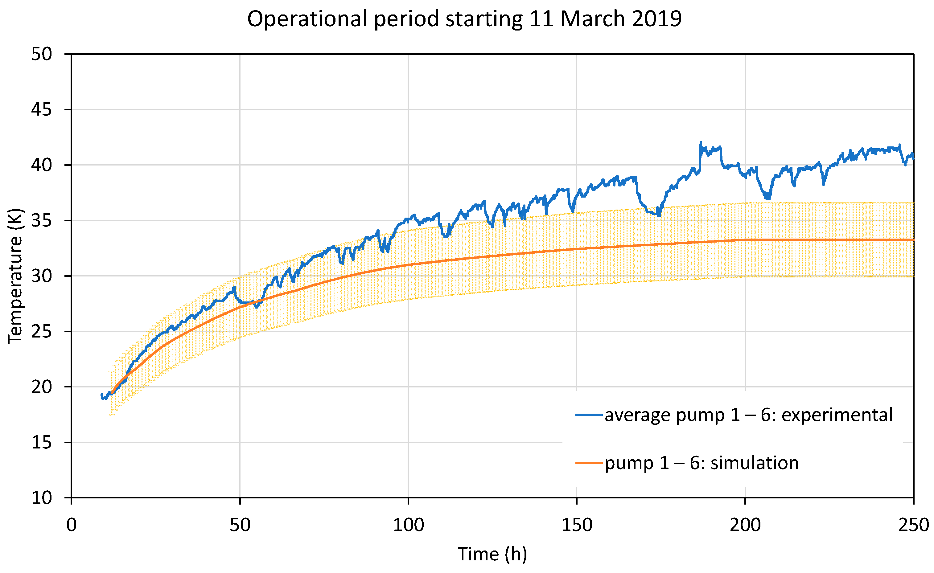
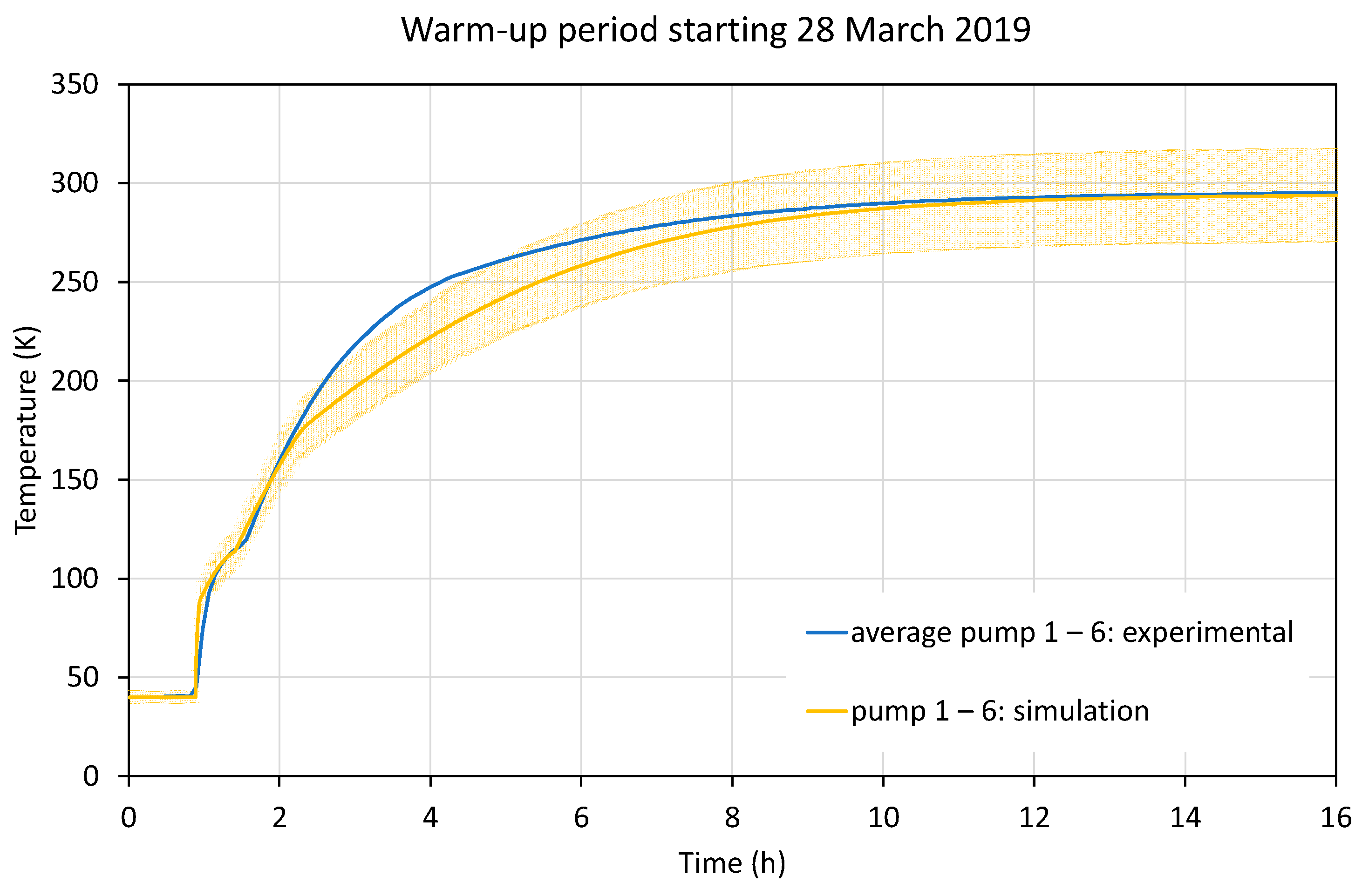
• Pumps 1–6: 6 round plates of 0.5 m diameter
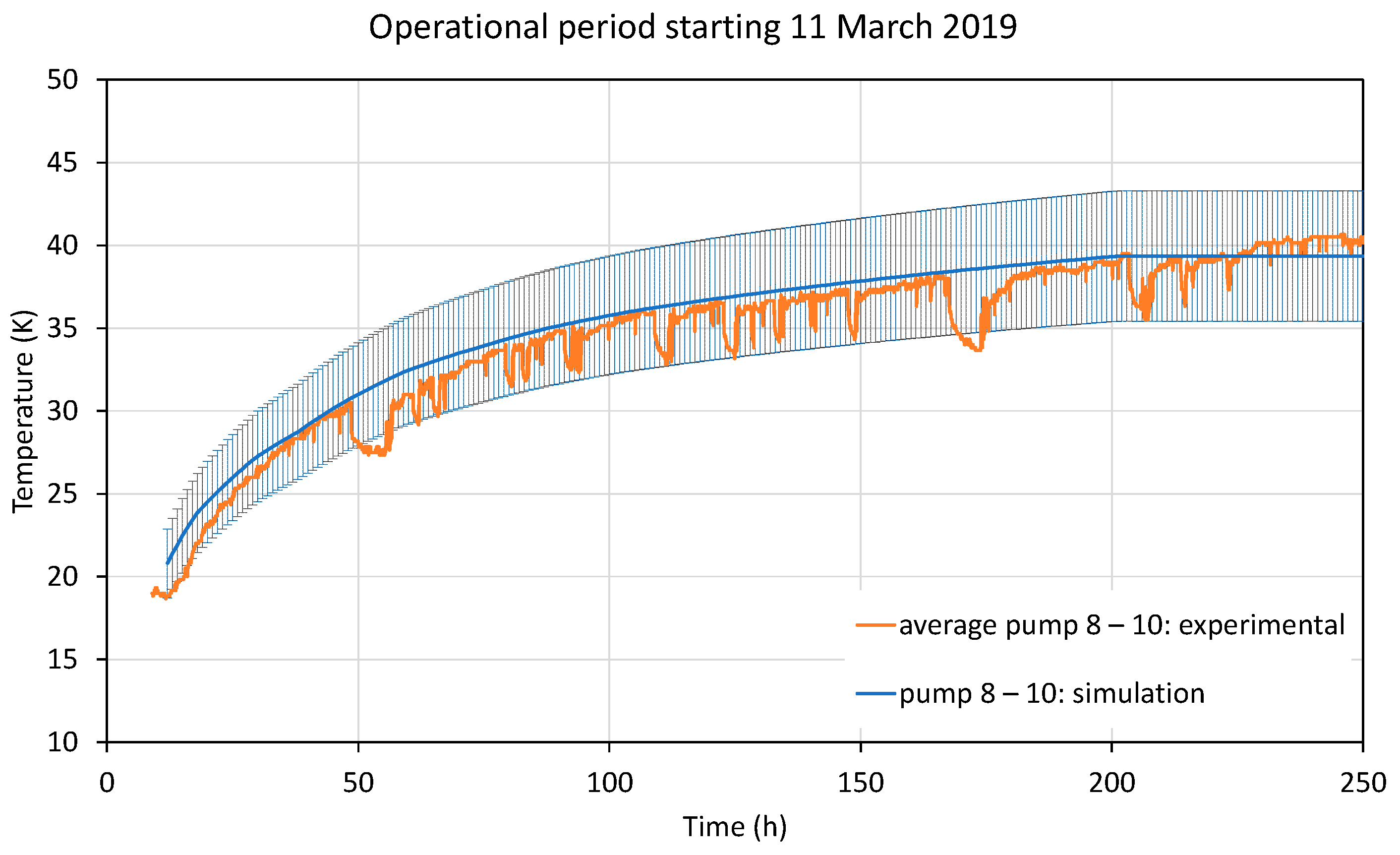
• Pumps 8–10: 3 square plates of 0.5 m × 0.5 m (pumps in place since chamber built)
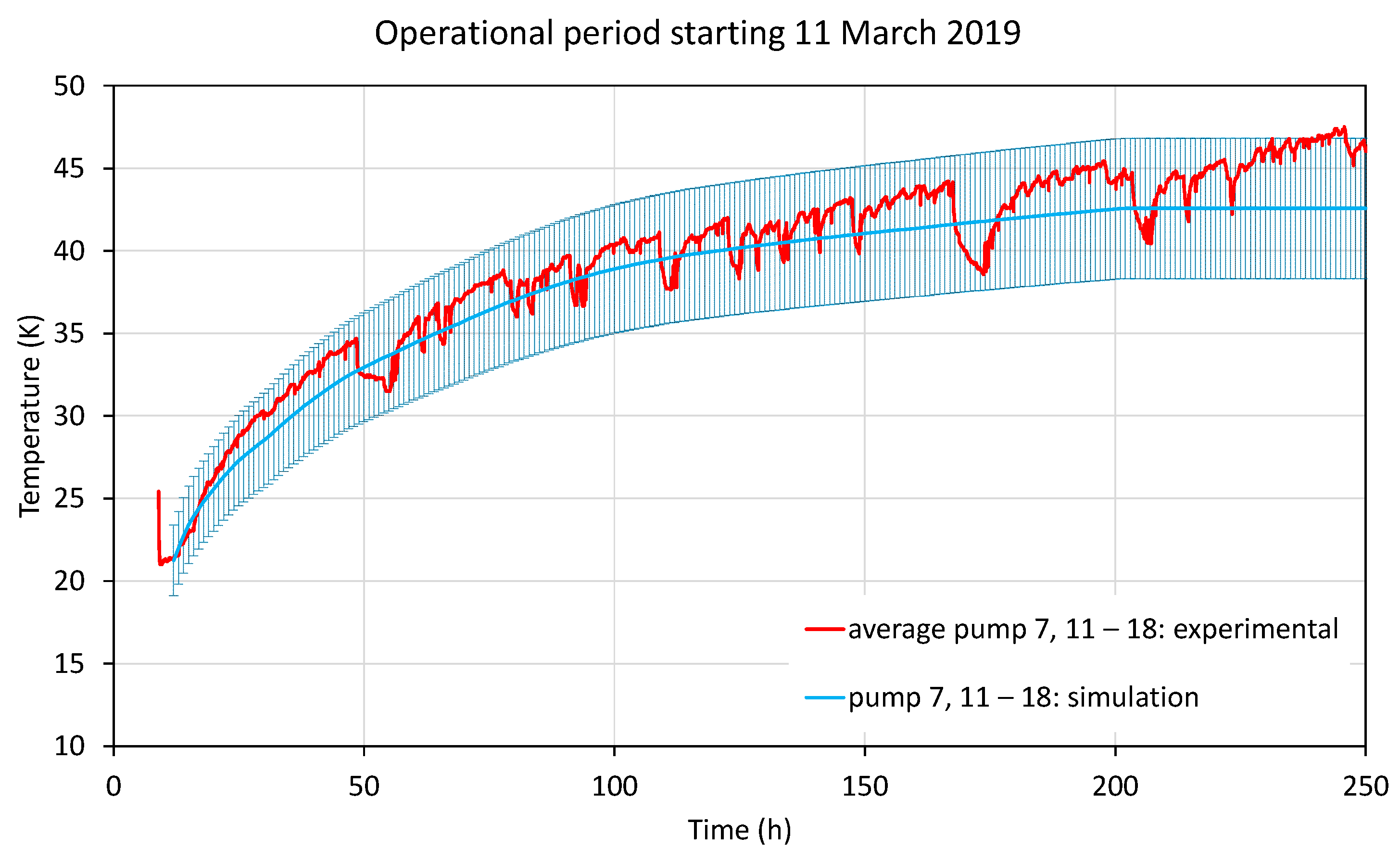
• Pumps 7, 11–18: 9 round plates of 0.6 m diameter

The initially used 0.5 m round plates have the smallest area and should show the best behavior with respect to cool-down. The large round plates have unprotected copper surfaces, and the others are nickel plated.

The next section shows the results of pumping speed tests for noble gases xenon, krypton, and argon. These gases may be used as propellants for space electric propulsion [8,11].

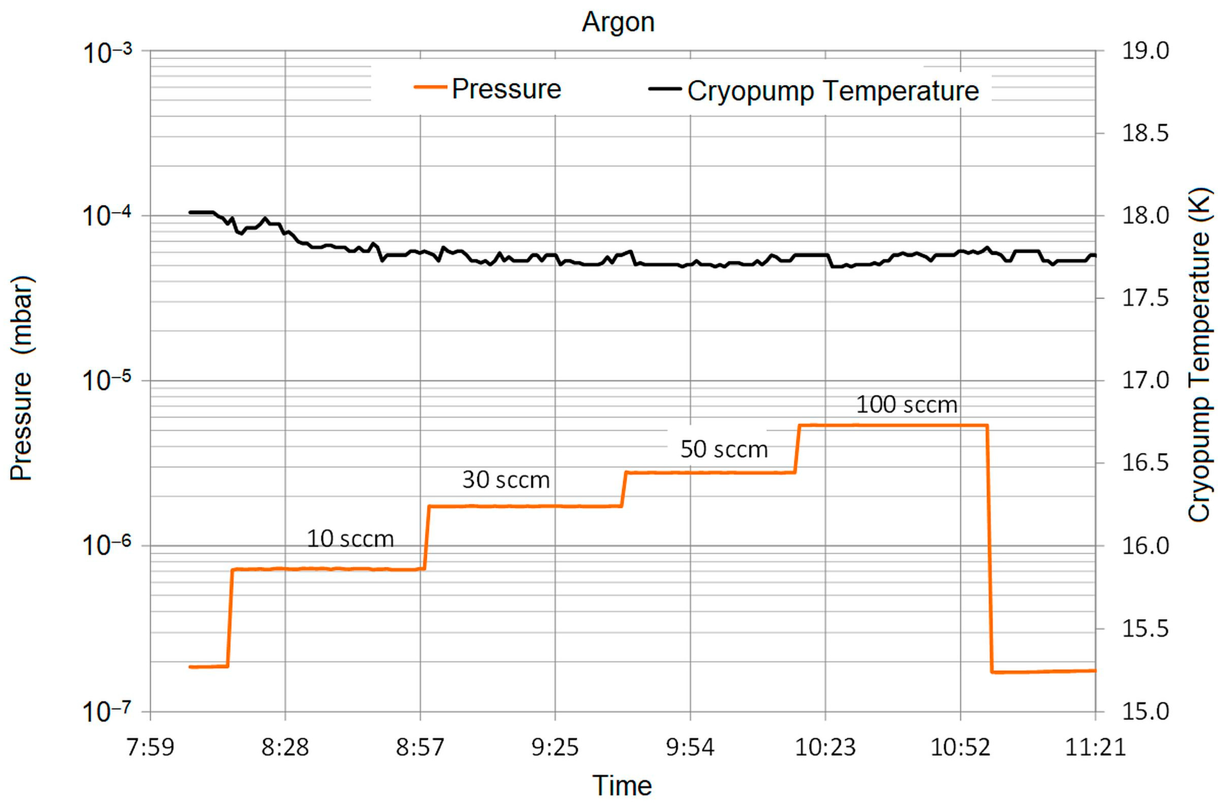
5. Pumping Speed Measurement

In order to characterize the performance of the facility, a pumping speed measurement campaign was performed. The measurements were carried out with freshly regenerated cryopumps, e.g., after having performed a complete warm-up cycle to room temperature for all cryopumps, while removing all evaporated gases with the mechanical pumps running. Following this step, after cool-down, the cold plates have the lowest possible temperatures that can be reached with the installed cold heads. Their temperatures went down into the range of 17–23 K. At these temperatures, the trapping of krypton and argon is possible. If temperatures increase above about 30 K, argon will not be trapped anymore, and the same applies to krypton above 40 K (see Figure 2).

This should be kept in mind when interpreting the pumping results shown in the next sections. As soon as gas is adsorbed, the plate emissivity will increase, which leads to an increase in temperature due to higher radiation loads.

The gas inlet simulating a running thruster for the pumping tests was a single pipe supplying cold gas into the vacuum chamber. Using a real EP thruster may give somewhat different results because the energy of the gas flow and its spatial distribution are different.

Determining a pumping speed S requires accurate flow measurement $q_L$ and pressure measurement p:

$$S\left(gas,e.g.Xe\right)=\frac{q_L}{p-p_{base}}in\frac{l}{s}$$

(1)

$p_{base}$ is the background pressure without propellant flow [18].

Pumping Speed Measurement for Xenon, Krypton, and Argon

The most relevant gas for electric propulsion today is xenon [7,8]. Therefore, the first pumping speed measurement presented here is for xenon. Figure 4 shows the chamber pressure development for xenon cold gas flows of 10, 30, 50, and 100 sccm. The pressure shown is nitrogen-calibrated, i.e., not corrected for xenon. Using a nitrogen pressure measurement is our practice and is accepted or even insisted on by facility users. The risk of confusion in data records is less, and pressure sensors have to work with propellant gas and without propellant during pump-down.

Additionally, one of the cryopump cold plate temperatures is shown in the diagram. During the measurement, its temperature stayed in the band of 18–19 K. In order to obtain stable conditions, the gas flow at each step was left on for about 30 min. The pumping speed was calculated using Equation (1) and the calibration factor was applied to the pressure measurement at gas flow. The resulting xenon pumping speed was as follows:

$$S_{Xe}=\mathrm{276,000}\frac{l}{s}$$

Figure 5 shows the pumping test with krypton cold gas feeding (gas flow: 10, 30, 50, and 100 sccm). With the same process as shown above for xenon, the krypton pumping speed was as follows:

$$S_{Kr}=\mathrm{360,000}\frac{l}{s}$$

Argon has the lowest condensation temperature of the above-mentioned gases, and the cryopumps are at their limit when pumping argon. Figure 6 shows the pumping test with argon cold gas feeding (gas flow: 10, 30, 50, and 100 sccm). With the same process as shown above for xenon, the argon pumping speed can be deduced as follows:

$$S_{Ar}=\mathrm{452,000}\frac{l}{s}$$

Of course, the lower the condensation temperature of a gas, the shorter the time span of the given pumping speed. This is due to the fact that the pumping cold surface will warm up during operation and the condensation of the working gas will come to an end.

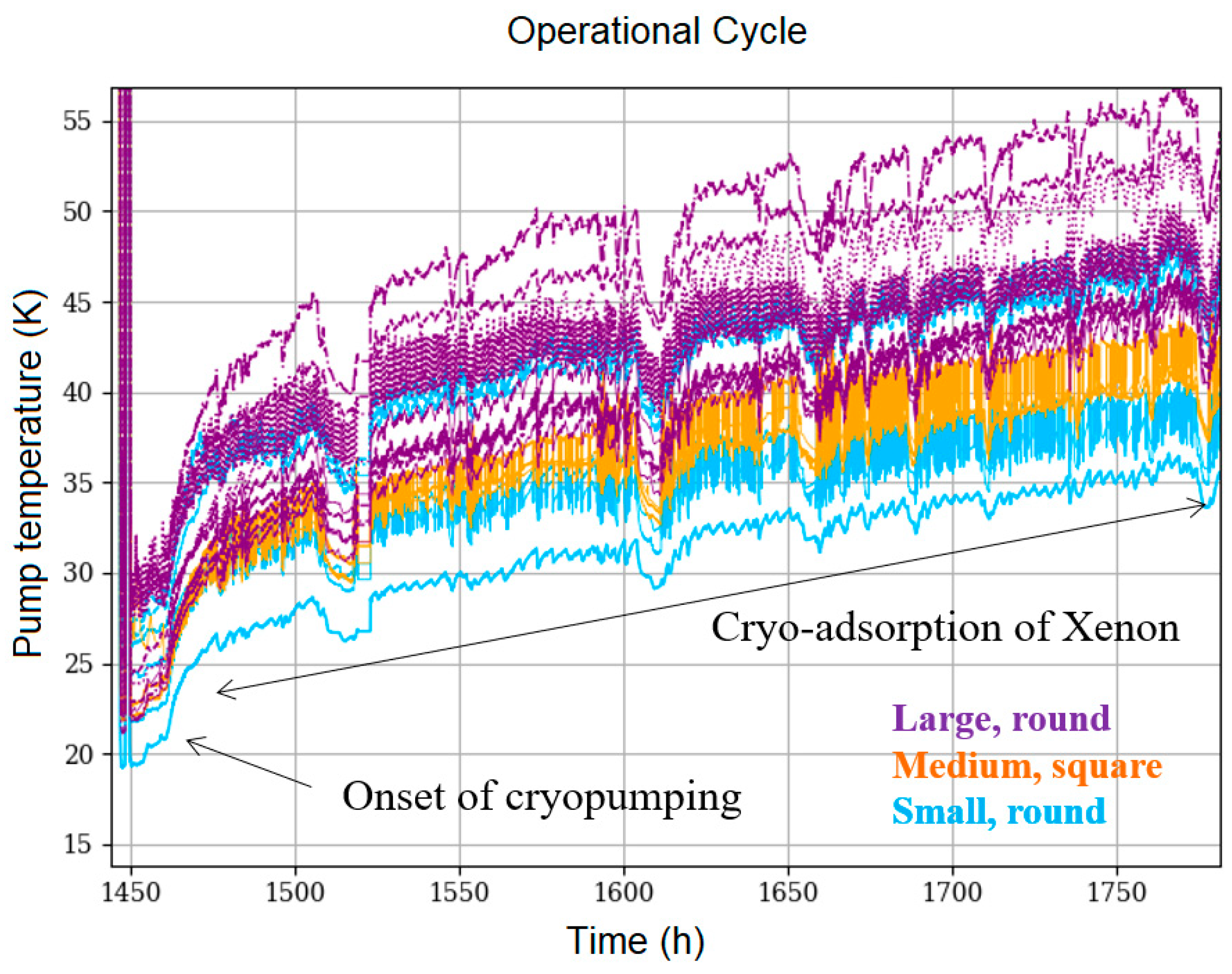
6. Cryopump Operation Analysis

At DLR’s facility, the cryopumps have cold plates of different sizes and shapes. This leads to different temperatures and a non-uniform behavior over longer pumping times. Figure 7 shows a typical cryopumping operation period of 12 days. After an initial cool-down, the cold plates reach 17–23 K. The plates slowly warm up during operation, which is due to gas adsorption and changes in emissivity. It can be seen that the small round plates have the lowest temperatures, and the largest plates show the highest temperatures. Between them, there are the square plates. There is an overlapping, and the temperatures are quite scattered.

Regarding temperature measurement accuracy, the sensors are of the PT1000 type, class B. This gives an error of <±0.5% at room temperature and about of <±5% at 30 K. Therefore, the temperature scattering may not be attributed to erroneous temperature measurement but to the spread of pump specifications, to different initial emissivities, to dirt and differences in polishing, and to differences in orientation and location in the chamber. In this figure, all the temperatures are still in the xenon pumping regime.

After the end of an operational phase, the cryopumps are switched off and the trapped gases are released. Such a warm-up cycle is shown in Figure 8. On average, the largest plates show the slowest warm-up. The square plates show the fastest warm-up, although there is an overlapping. A cryopump model should be able to model the temperature features present during operation and warm-up.

7. Cryopump Modelling

Cryopump operation is very expensive with respect to electrical energy and cooling water consumption. Therefore, being able to optimize pump shape, cold plate material, and pump placement in a chamber is crucial for cost optimization. Furthermore, a good operating strategy can reduce costs and increase intervals between regeneration. Testing different setups in a large facility is often prohibitive due to high costs and long testing times. Optimization via modelling is a better choice for design and also, later, for operation.

The physics of condensation processes at the cold plate surface of a cryopump is complex and depends on many parameters. The condensation includes different gases at the same time, may generate various ice lattice structures, and may depend upon the surface microstructure and cleanliness of the cold plate as well. Cryopumping is a typical subject for several areas in science, e.g., particle physics or very low temperature or fusion research, and references can be found [19,20,21,22].

The literature about typical issues when performing electric space propulsion testing and good and proven practices on system design is less abundant, e.g., pages 18 ff in [14,15,23,24]. Therefore, designing or optimizing a pump system is not straightforward; additionally, all facilities are unique.

In order to compile input for an EP pumping system, the following sections elaborate parameters like pump cooling capacity, and material and gas properties.

7.1. Cryopump Head Cooling Capacity

Firstly, a dynamic model of cryopumps must include the amount of heat that the pump device can remove. This capability strongly depends on its operating temperature. As an example, the cooling power of a cryopump cold head type CoolVac CP140T, powered by a compressor Coolpak 6000H (both from Leybold GmbH, Koeln, Germany) can be schematically seen in Figure 9. This graph is based on manufacturer-given data in its datasheet. The cold head of the pump system can dump about 220–230 W of heat at room temperature, and can remove about 45–50 W at 25 K. The pump can cool down to about 15–20 K. By reducing to such a low temperature, this type of pump is able to adsorb/pump gases like nitrogen, oxygen, and argon. One should mention that these are only sample data, and the real cooling capacity may vary, e.g., depending on cold head orientation or cooling water temperature.

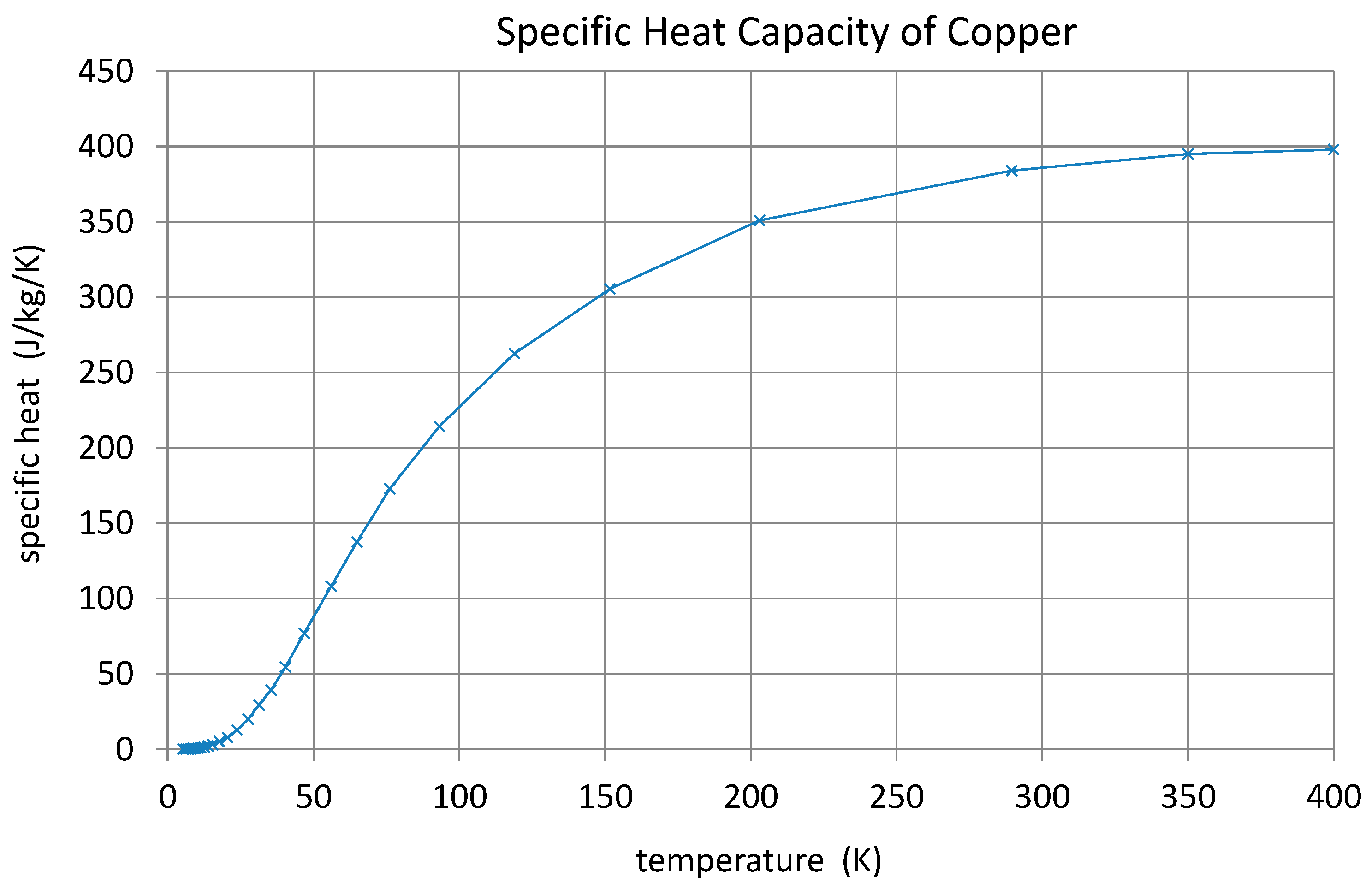
7.2. Cold Plate Material Properties

As shown in Section 3, a single stage cryopump has a large metal plate attached to its cold head. This plate is cooled down to cryogenic temperatures, and condenses and adsorbs gases. The material of such a plate is typically copper. The material properties of copper and its definitions were extracted from [25,26,27]. For the highest thermal conductivity, the copper used must be very pure and oxygen-free. This purity can be characterized by the Residual Resistivity Ratio (RRR), which is defined as the ratio of the resistivity of the material at room temperature compared with the resistivity close to 0 K.

Figure 10 shows the thermal conductivity of copper with various purity grades. One can see that using very pure copper (RRR = 2000) can increase thermal conductivity by a factor of 1.5 at 60 K, 2 at 40 K, and even 15 at 20 K. High RRR values are the best choice for cryogenic pumping tasks.

Besides thermal conductivity, specific heat is important when it comes to the cooling behavior and cool-down times of pumps. Reference [26] was used to create a simplified model for the specific heat $c_p$ of copper for temperatures between 10 K and 400 K, which is the region of interest for this application. In the reference, $c_p$ is given in $\frac{J}{mol·K}$, and

Table 1. Approximation functions for copper specific heat.

Temperature Range (K)	${\mathit{c}}_{\mathit{p}}\left(\frac{\mathit{J}}{\mathit{m}\mathit{o}\mathit{l}\times \mathit{K}}\right)$
4.2–30	$c_p\left(T\right)=6.94\times {10}^{-4}T+4.76249\times {10}^{-5}{T}^3+1.05866\times {10}^{-9}{T}^5+1.0287\times {10}^{-10}{T}^7-1.68191\times {10}^{-13}{T}^9+9.0127\times {10}^{-17}{T}^{11}-1.13003\times {10}^{-20}{T}^{13}$
30–50	$c_p\left(T\right)=4.13788-0.457798T+1.73771\times {10}^{-2}{T}^2-1.81035\times {10}^{-4}{T}^3+6.57663\times {10}^{-7}{T}^4$
50–70	$c_p\left(T\right)=-3.44481+2.71874\times {10}^{-2}T+5.82694\times {10}^{-3}{T}^2-5.9299\times {10}^{-5}{T}^3+1.76354\times {10}^{-7}{T}^4$
70–100	$c_p\left(T\right)=-11.5255+0.41885T-1.13549\times {10}^{-3}{T}^2-5.92034\times {10}^{-6}{T}^3+2.93875\times {10}^{-8}{T}^4$
100–200	$c_p\left(T\right)=-15.14608+0.577212T-3.639869\times {10}^{-3}{T}^2+1.12101\times {10}^{-5}{T}^3-1.363615\times {10}^{-8}{T}^4$
200–298	$c_p\left(T\right)=6.33481+0.162424T-5.78862\times {10}^{-4}{T}^2+9.95052\times {10}^{-7}{T}^3-6.62868\times {10}^{-10}{T}^4$
298–1358	$c_p\left(T\right)=23.55055+6.89498\times {10}^{-3}T-2.95229\times {10}^{-6}{T}^2+1.78088\times {10}^{-9}{T}^3-\frac{84616.4}{T^2}$

lists the complete set of approximations. These formulae were used to calculate the specific heat of copper between 10 and 400 K. By using the molecular weight of copper of 63.546 g/mol for conversion to $\frac{J}{kg·K}$, the result is plotted in Figure 11. The shape shows the large difference between specific heat at cryogenic temperatures and its room temperature value. Lower specific heat capacity means that less energy is needed for changing temperature.

7.3. Water Ice Properties

The pumping process is based on the cryo-adsorption of gases and therefore the properties of relevant gases at their frozen state are important. Water ice, water vapor, and air constituent properties can be found in the standard literature, e.g., [28,29].

Concerning water ice, one very important property is its emissivity. Figure 12 displays data for water ice-layer emissivity versus layer thickness (see [30]). Even for a layer in the sub-mm range, the emissivity or radiation absorption approaches 1, which, in the case of our cryopump application, leads to high heat loads from a warm environment transferring onto a cyro-cooled surface with some ice layer on it.

Therefore, water vapor in the vacuum chamber, which is easily frozen onto cryopump surfaces, may cause issues with respect to radiation absorption. Cryopump layout and operational strategies should account for that. Furthermore, such effects should be kept in mind when thinking about thruster technologies based on water as a green propellant.

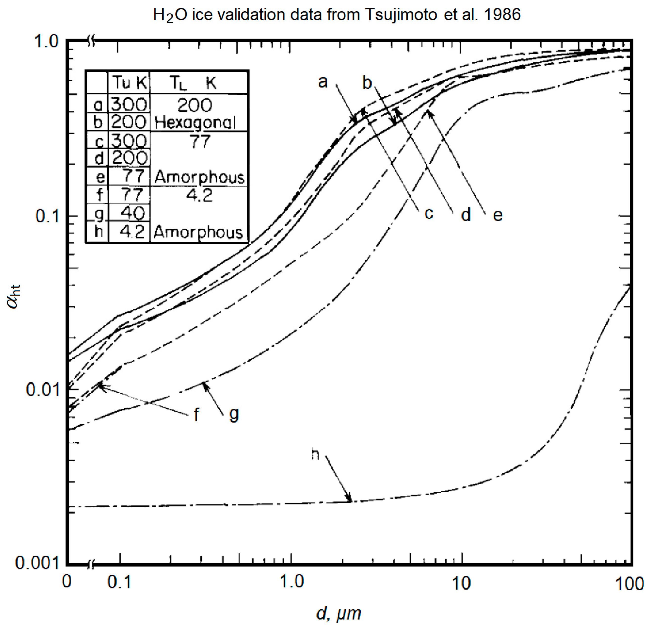
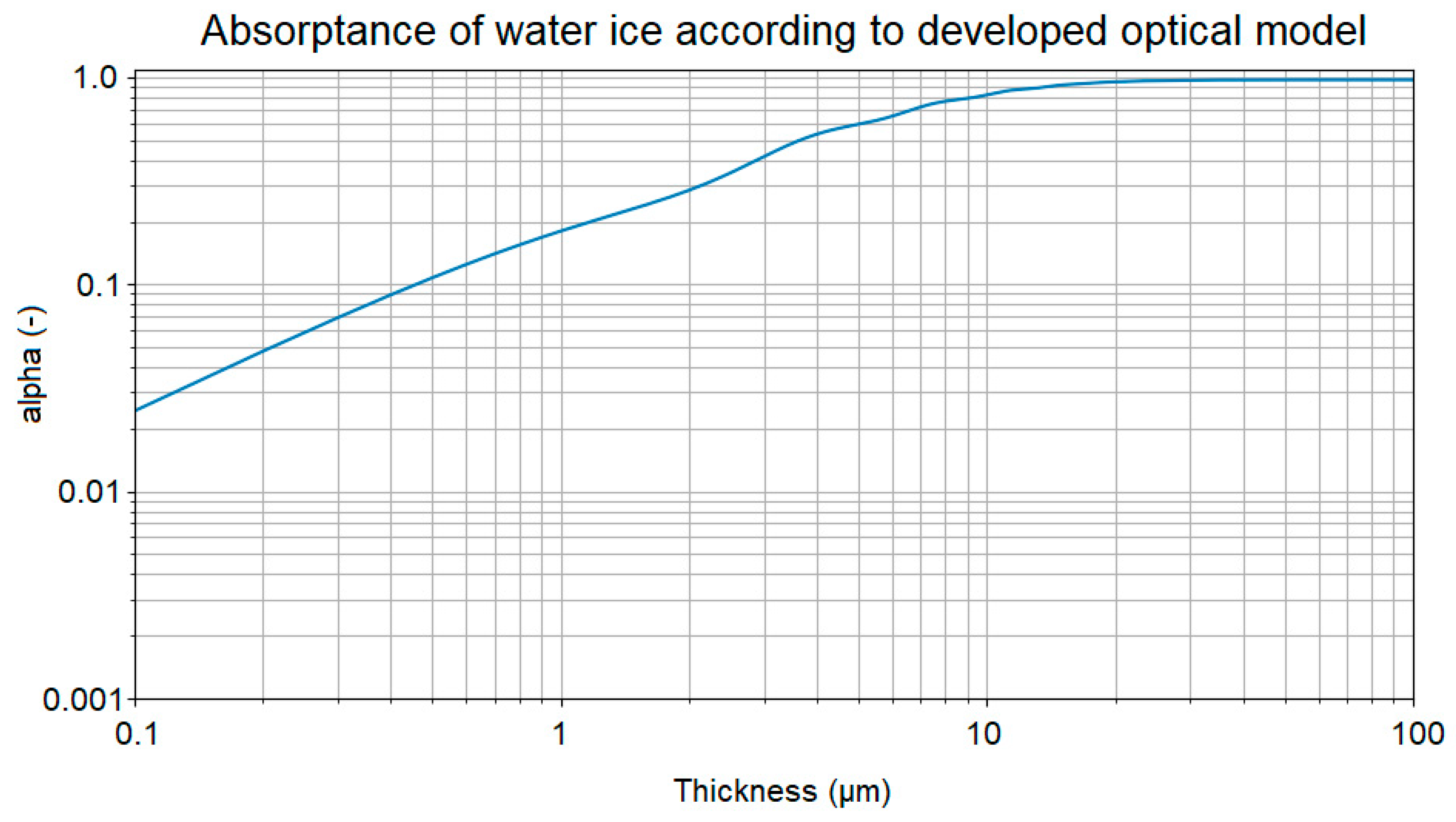
7.4. Ice Absorptance Profile Similarity Analysis

In general, the increasing radiation absorptivity profiles shown in most literature, such as Refs. [31,32], follow a rather smooth curve, which can also be seen in Figure 13 if the interference features are ignored. It can be observed that the profiles behave similarly, so that if the height of the deposit and its absorptance are normalized by their maximum values, alpha_max and h_max—i.e., the value of the deposit height where optical thickness is achieved and the value of absorptance which is asymptotic—the profiles have a similarity. This can be clearly observed when comparing the profiles of water ice deposit absorptance and CO₂ ice deposit absorptance. Even though these two deposits display very different profiles in terms of critical thickness and maximum absorptance, when normalized, the profiles are similar, as seen in Figure 14. Indeed, the profiles shown in Figure 14 can be fitted using a two-component function, with a power profile in the first half and a logarithmic profile in the second.

The function components were generated in such a way that the resulting function would be exact at the edges ($\overline{\propto }$= 0 and 1 at $\overline{h}$ = 0 and $\overline{h}$ = 1, respectively) and so that it would be continuous and smooth in its first derivative. The following expression was found:

$$\overline{\propto }\left(\overline{h}\right)=\left\{\begin{array}{c}{ \overline{h}}^{ 0.48}+0.86585 \overline{h}-1.15414 {\overline{h}}^2 if \overline{h} \le 0.5\\ 0.2\ln \left(\overline{h}\right)+1 otherwise\end{array}\right.$$

The relative error of the above function when evaluating for both water and CO₂ ice is less than 15%, even <3% for relative thickness levels greater than 0.75. This is a good fit considering that even the input data from water and CO₂ ice have this level of uncertainty.

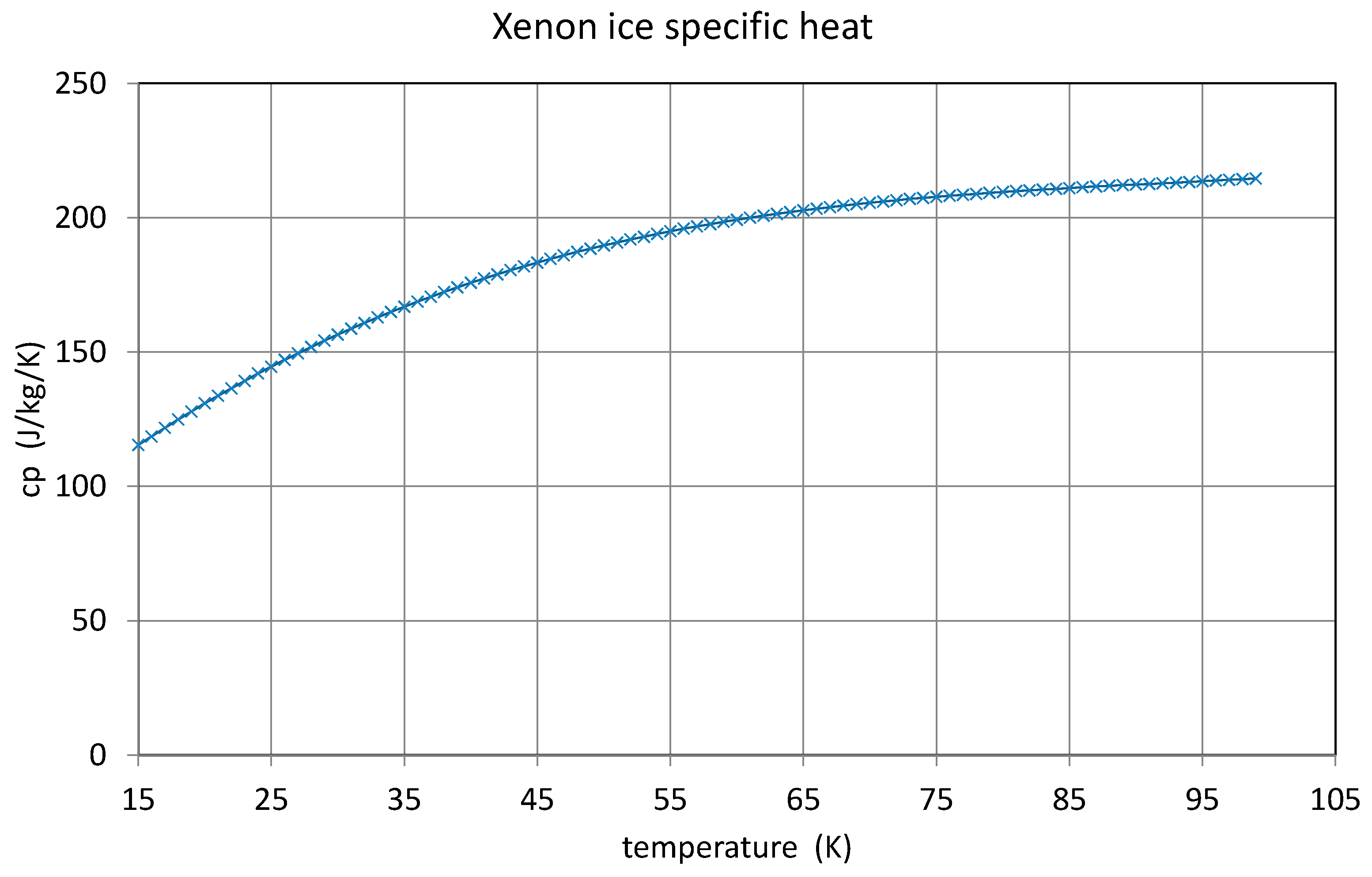
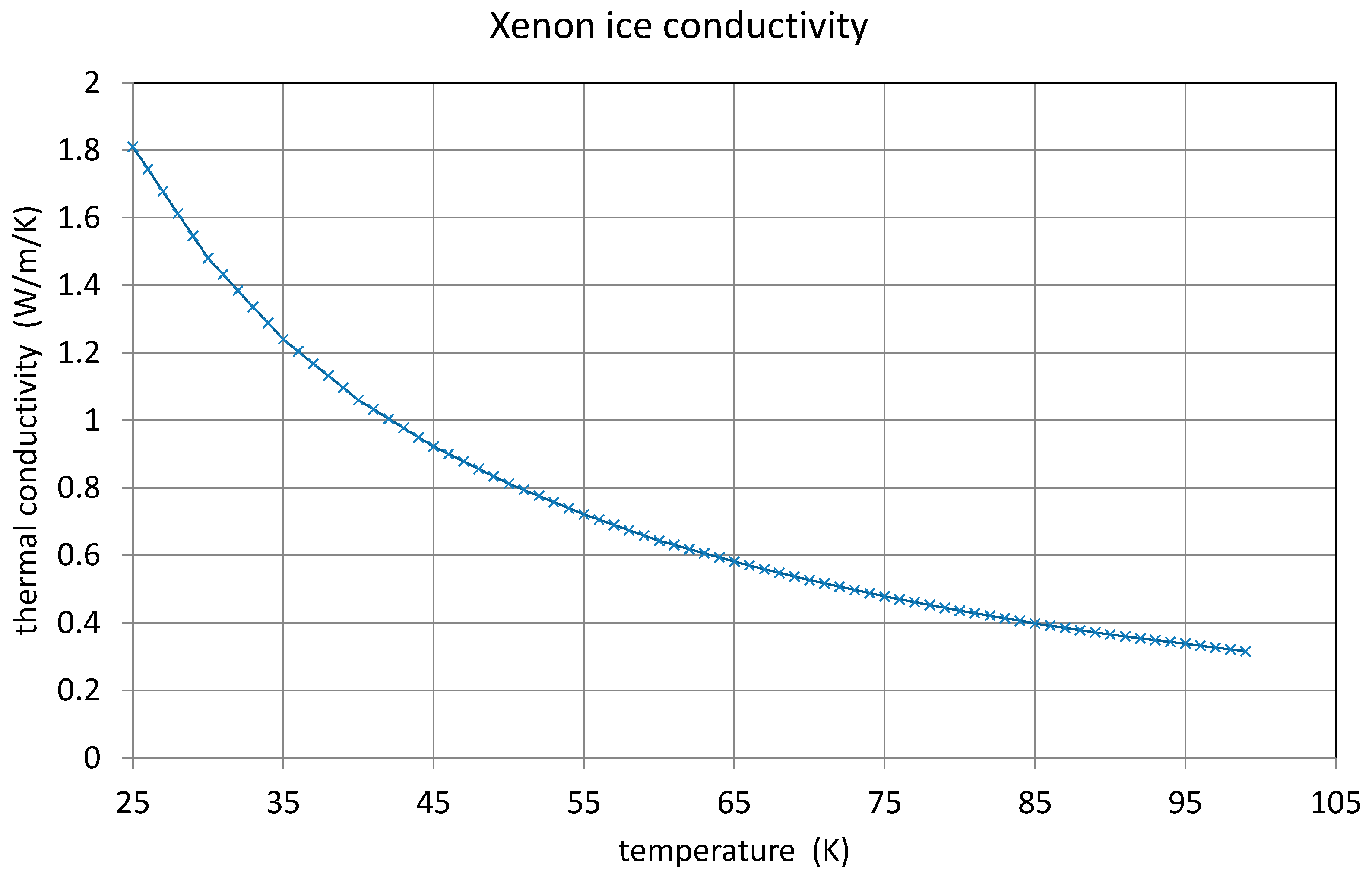
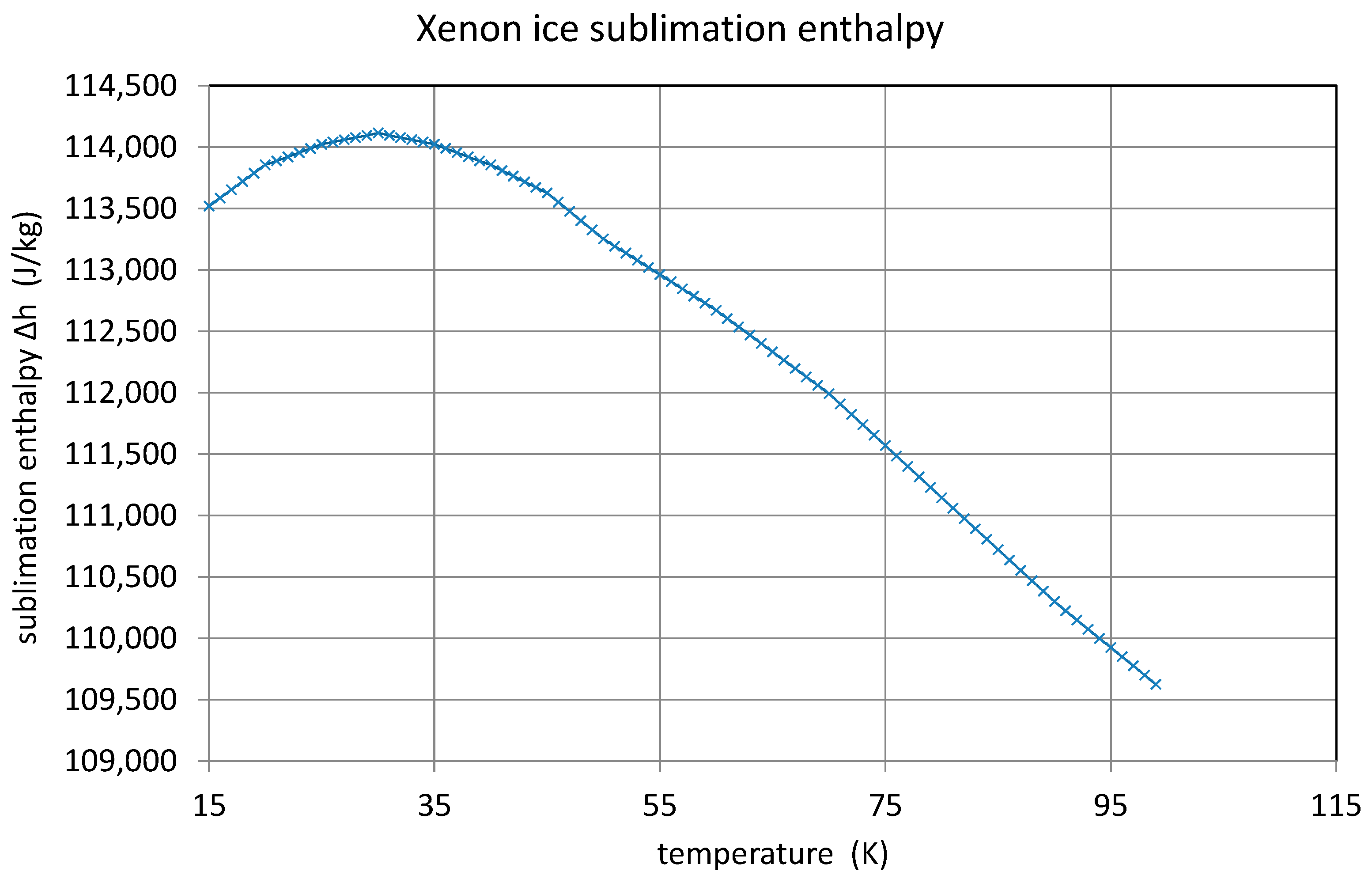
7.5. Xenon Ice Properties

The literature data for a noble gas like xenon at cryogenic temperatures are not very abundant. The following gas property plots were generated based on data published in [32,33,34]. Figure 15 shows the density of xenon ice. This parameter is of importance for the estimation of weight on a cold plate after longer operation. This is required for not exceeding the maximum mechanical load capacity of the pump cold head. It is also important for determining the total heat capacity of the xenon layer.

Figure 16, the xenon ice-specific heat at low temperatures, shows that adding a certain ice mass onto the copper cold plate changes the temperature–time response because the xenon ice-specific heat is of the same order of magnitude as the copper, or even higher. Figure 17 displays xenon ice thermal conductivity, which is low compared with the copper. Therefore, a certain ice thickness will limit the heat transmission capability and, with that, the pumping speed of the cold surface. One may think that the deposition or de-sublimation of xenon gas on a cold surface will add a noticeable amount of energy to the energy budget. Looking a Figure 18, we see that xenon has a sublimation enthalpy of about 1.14 × 10⁵ J/kg for low temperatures. With a mass flow in the order mg/s the heat flow power is about 3 mW. This figure is negligible at 30 K, where the pump can dump about 50 W.

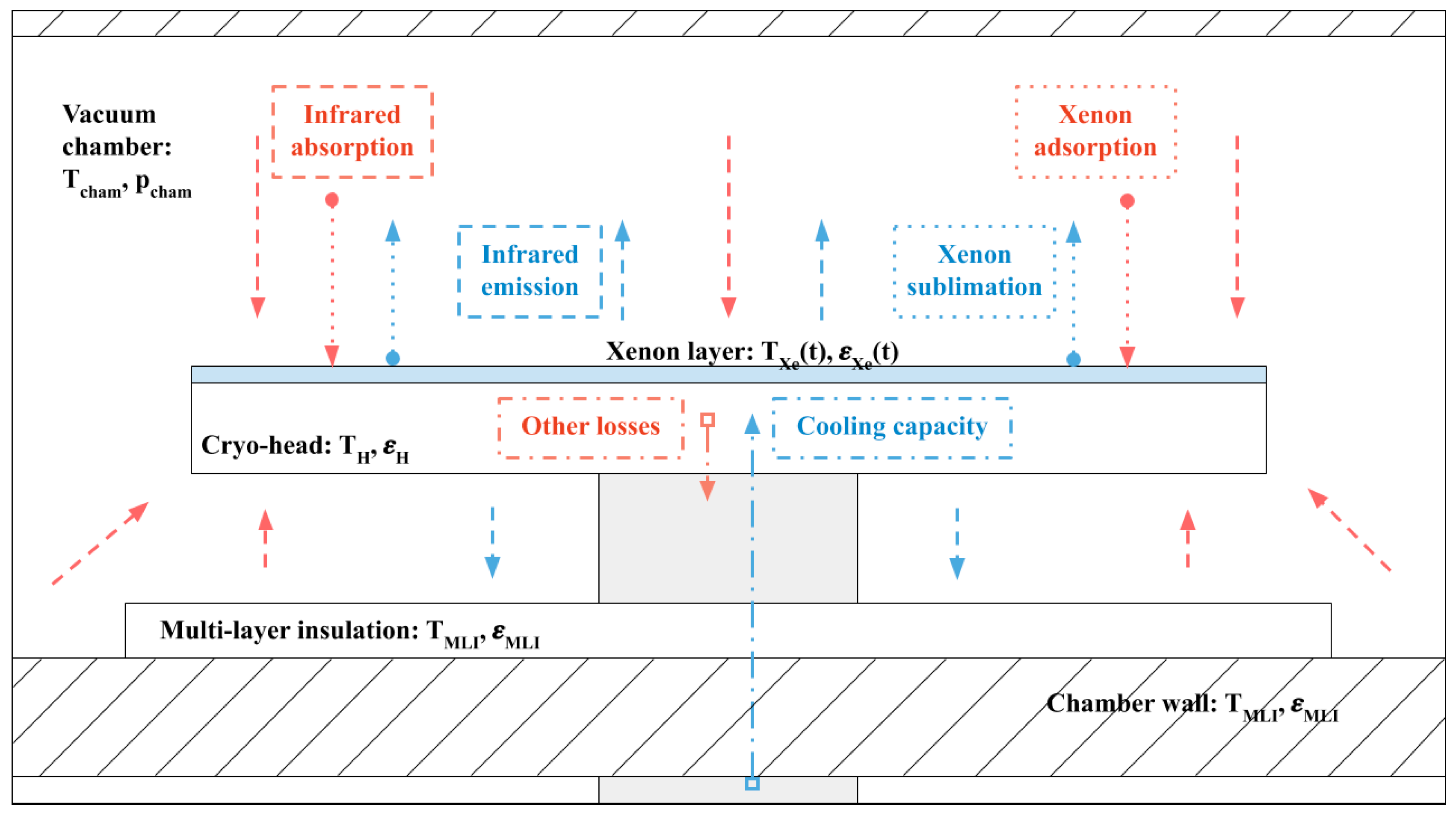
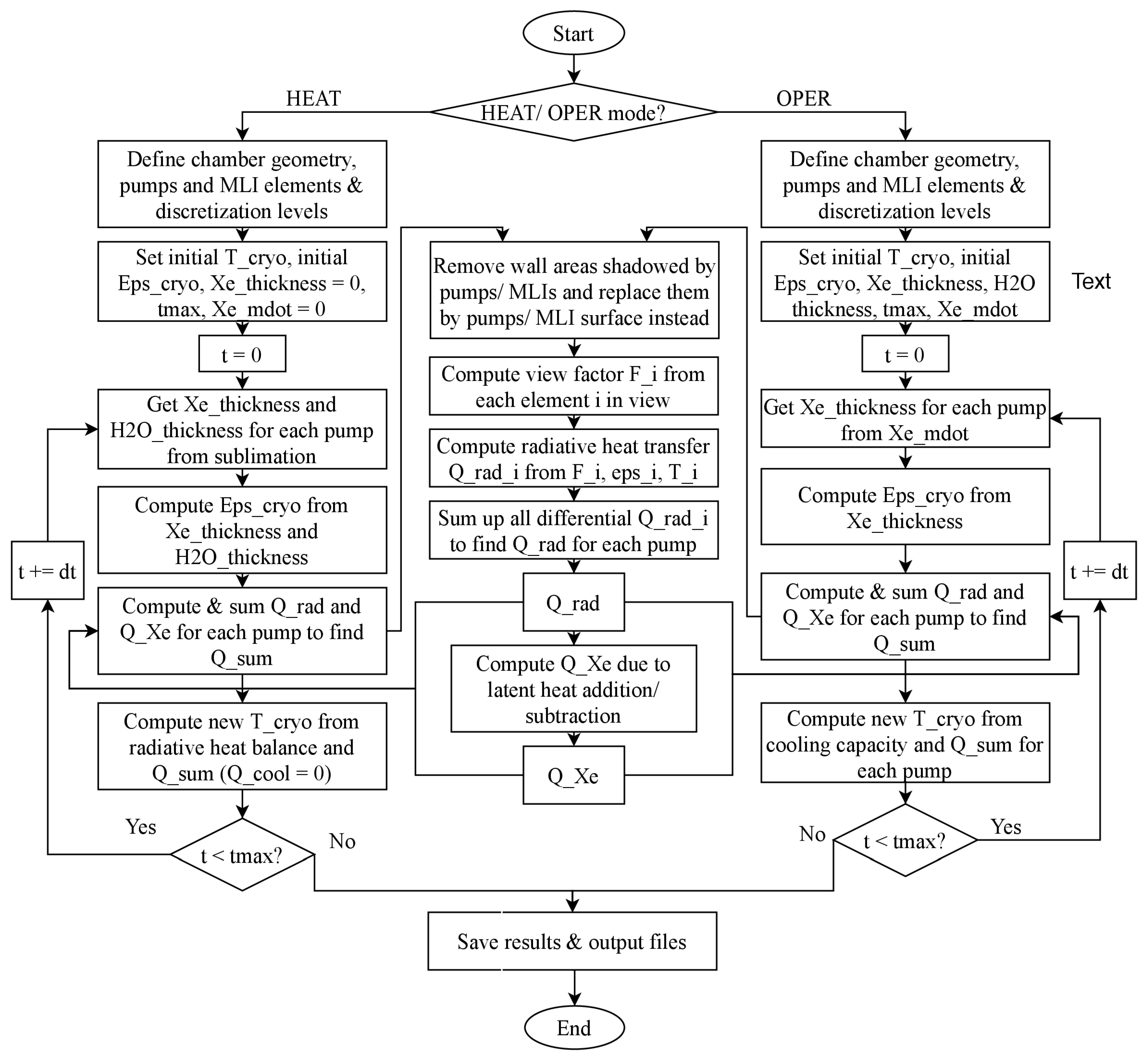
7.6. Model for Operation Simulation

The basic thermodynamic processes around a cryopump can be seen in Figure 19. The radiation exchange between the pump plate, the chamber wall, and the inner components is defined by the emissivities of the cold plate, the condensate layer, and the chamber wall properties.

During operation modelling, the thruster is running and may constitute an additional heat source. Usually, the temperature distribution on a thruster enclosing surface is very type-dependent, and is known only to manufacturers (intellectual property). But if we assume a reasonable homogeneous thruster temperature of, e.g., 300 °C, we obtain about kW/m² blackbody radiation compared with the 400 W/m² from the chamber walls at room temperature. The thruster heat source may have an area of 0.1 m² (0.3 × 0.3 m²), and is located at distances of 2.5–4 m from the cryopump cold plates. This geometry provides a hot body with a radiation contribution coming from a solid angle fraction of <0.0014, which increases the total heat radiation by a few percent (assuming a chamber at room temperature). Therefore, in this approach, we omitted the thruster as a heat source, and it is modelled only as a cold gas source releasing xenon into the chamber.

A model must take into account that the emissivities of cold plates and ice layers change during cryo-trapping or evaporation. For the DLR model, a full 3D, time-dependent numerical simulation was set up to properly resolve the instantaneous heat balance for each pump and therefore its resulting temperature, including the zonal method to properly account for the radiative heat transfer. The zonal method is an intermediate simulation method between a single zone model, which is far too coarse for modelling chambers and cryopumps, and a fine mesh finite element method, which splits the space of interest into millions of small grid elements. The latter would require computational resources not available for this investigation. Zonal methods are often used in computational fluid dynamics.

The geometry of the chamber was represented by a cylindrical body enclosed by two spherical caps, discretized to consist of very small planar elements for the zonal method calculation. The pumps were modelled as 2D surfaces oriented such that their normal pointed towards the centerline of the chamber. The heat flow at the contact between the cryopump cold head and the cold plate was set as ideal, as we observed that cold head and plate temperatures are usually very close.

For each pump, the calculations were carried out separately to track the instantaneous pump heat balance, temperature, and thickness of the ice layers. The temperature was set either to room temperature for the cool-down simulation or the final measured temperature before the shut down for the heat-up cycles.

The numerical simulation modelled the following energy balance:

$$Q=Q_{rad}+Q_{cond}+Q_{Xe}+Q_{H2O}=Q_{cool}+Q_{dT pump},$$

(2)

where the first term is the heat transfer due to radiation, the second due to conduction, the third due to cryo-deposition and the warming of the xenon, and the fourth term due to the cryo-deposition and the warming of the water vapour (if applicable). On the righthand side, this is balanced by the cooling power of the pump and the heat capacity of the pump. Since this is dictated by the new pump temperature, the pump temperature at the next time step was derived from this value. The contributions will now be described in further detail.

Firstly, the cooling capacity is known from the specification provided by the manufacturer. While the specification gives the ideal cooling capacity, this does not apply for pumps that have been in operation for months or several years. A lesson that we learned during years of facility operation is that a cryopump might work reliably over years, while others may rapidly loose cooling capacity after a few months. This also happened after fresh refurbishments carried out by the manufacturer. One mechanism for this is the wear of valves and pump pistons inside the cold head.

As these effects are not easy to quantify or predict, using the manufacturer data must suffice as an indication of the expected performance. Dedicated tests could be conducted in a controlled environment to measure this deteriorated capacity for each pump separately. However, such tests would be very time consuming and would demand significant financial resources.

The heat capacity of a pump is simply given by the following:

$$Q_{dT pump}=m_{pump}{c}_{p,pump}dT$$

(3)

where $m_{pump}$ refers to the mass of the pump, $c_{p, pump}$ refers to the specific heat capacity of the pump material, and $dT$ to the temperature difference in the pump between the two consecutive time steps. In this context, the pump refers to the pump head only (as due to heat conductivity and a relatively narrow throat, it is assumed that heat is not conducted to the rest of the pump effectively).

The radiative heating term was determined from a separate numerical radiation simulation using the zonal method. For two surfaces of radiosities, $J_1$ and $J_2$, the radiative heat transfer from 1 to 2 is given by the following:

$$Q_{rad,12}=A_1{F}_{12}(J_1-J_2)$$

(4)

in which $F_{12}$ is the view factor from surface 1 of area $A_1$ to surface 2 of area $A_2$. The radiosities can be determined from the Oppenhaim’s electric circuit analogy for heat exchange between two bodies with the consideration of space and surface resistances, giving the following:

$$\frac{\sigma {T_1}^4-J_1}{R_1}-\frac{J_2-J_1}{R_{12}}=0$$

(5)

$$\frac{\sigma {T_2}^4-J_2}{R_2}-\frac{J_1-J_2}{R_{21}}=0$$

(6)

where the space and surface resistances are given as follows:

$$R_{12}=\frac{1}{A_1{F}_{12}},R_{21}=\frac{1}{A_2{F}_{21}},R_1=\frac{1-{ϵ}_1}{A_1{ϵ}_1},R_2=\frac{1-{ϵ}_2}{A_2{ϵ}_2}$$

(7)

This results in a system that can solve for $J_1$ and $J_2$, once the view factors are properly calculated. The calculation of the view factors is performed in a differential fashion. As mentioned above, the walls of the chamber, as well as the surface of the pumps, are split into small planar mesh areas, while the surface normal vectors are calculated a priori. Then, for each combination of these planar cells, the mutual view factor is computed through the following:

$$F_{12}=\frac{1}{A_1}\iint \frac{cos{\theta }_{2}cos{\theta }_1}{\pi {\left|{\underset{\_}{\mathit{r}}}_{12}\right|}^2}d{A}_{1}d{A}_2$$

(8)

The angles ${\theta }_1$ and ${\theta }_2$, which are the viewing angles, can be readily calculated from the vector between the two areas, ${\underset{\_}{\mathit{r}}}_{12}$, and the surface normals as follows:

$${\theta }_1=arccos\left(\frac{{\underset{\_}{r}}_{12}{\underset{\_}{n}}_1}{\left|{\underset{\_}{\mathit{r}}}_{12}\right|\left|{\underset{\_}{\mathit{n}}}_1\right|}\right),{\theta }_2=arccos\left(\frac{{\underset{\_}{r}}_{12}{\underset{\_}{n}}_2}{\left|{\underset{\_}{\mathit{r}}}_{21}\right|\left|{\underset{\_}{\mathit{n}}}_2\right|}\right)$$

(9)

Next, the conductive heating term would be defined according to the temperature gradient along the pump with some proportionality constant $\lambda$, depending on geometry and material characteristics:

$$Q_{cond}=\lambda dT/dx$$

(10)

but since insufficient information was available to estimate the magnitude of this constant, conductive heat flux was neglected. It is expected that it would be by an order of magnitude smaller than that of, for example, the radiative heat flux in almost any conditions.

Finally, the heating due to xenon cryo-deposition and sublimation can be expressed as follows:

$$Q_{Xe}=C_s[m_{Xe,gas}{c}_{p,Xe,gas}\left(T_{gas}-T_{subl}\right)+d{H}_{subl}+m_{Xe,solid}{c}_{p,Xe,solid}(T_{subl}-T_{pump}\left)\right],$$

(11)

where $C_s$ refers to the capture coefficient indicating how much of the incoming xenon is captured on the pump. The same formula can also be used to calculate $Q_{H2O}.$ The capture coefficient was treated to be 1 in this work, until the xenon ice layer thickness was large enough to prevent any further cryo-adsorption due to the poor thermal conductivity of the xenon ice. Then, no further ice attachment was possible, effectively setting $C_s$ to 0.

The largest source of uncertainties in the calculations above, next to the cooling capacity of the pumps, are the initial and final optical properties of the pumps. The optical properties are not accurately known in the “clean pump state” nor after the water and xenon ice has deposited on them.

The emissivity of the “clean” pump surface differs per pump due to surface material, degradation and contamination. This emissivity can be, in theory, estimated during the heat-up process of the pumps (when the chamber is still closed) at high enough temperatures when the water vapour is released.

The optical thin film properties of water ice are relatively well known ([29,30]). These properties are needed in the infrared portion of the spectrum, where the chamber radiates predominantly. What is required for this numerical simulation is the surface emissivity of the water ice thin film as a function of the film thickness. The data from Ref. [28] were used, and a power/logarithmic fit was made to simplify modelling. This fit was based on combined data for CO₂ and H₂O ice through similarity analysis. The fit reads as follows:

$$\begin{array}{c}\frac{a}{a_{max}}=({\frac{h}{h_{max}})}^{0.48}+0.86585(\frac{h}{h_{max}})-1.15414(\frac{h}{h_{max}}{)}^2 \mathrm{for} \frac{h}{h_{max}}<0.5\\ \frac{a}{a_{max}}=0.2ln\left(\frac{h}{h_{max}}\right)+1 \mathrm{otherwise},\end{array}$$

(12)

in which the values with the subscript “max” correspond to the maximum expected height and absorption coefficient value that can be achieved.

A mesh convergence study was performed on the number of mesh elements of both the chamber walls as well as the pumps. It was observed that in order to stay within 5–10% errors, approximately 10⁵ chamber wall elements were required. The reason why such a large number of elements is needed is the fact that the chamber wall also contains the simulated MLI surfaces. The MLI surfaces have different properties than the chamber wall and significantly reduce the heat flux towards the pump. Thus, a coarse discretisation means that the MLI surfaces, which are relatively small compared with the entire chamber and which play a major role in radiative heat transfer, are not accurately represented. In addition, for each pump, 50 planar elements were considered on both sides to achieve accurate values. In summary, Figure 20 shows the block diagram of the model. It includes the two branches, one for the pump operation, and one for the regeneration/warm-up phase.

8. Comparison of Data and Model

8.1. Data Set

The data used in the following section for comparison with the simulation model stem from a facility operation interval in March–May 2019. This data set contains several operational periods with consecutive cryopump warm-ups. One operational period of about 10 days, starting 11 March, with thruster gas flow, and the following pump warm-up, starting 28 March, were extracted.

Regarding temperature measurement accuracy, the above-mentioned errors of <±0.5% at room temperature, and about of <±5% at 30 K are valid. The mass flow of the thruster is known, with an accuracy of ±3%, and it is assumed to be constant during an operational cycle.

8.2. Modelling Operation

The following model versus data comparison was undertaken for a facility operation with a thruster running at 50 sccm xenon mass flow, and the respective xenon deposition on each pump. Concerning data, the viewing factors of each pump were not the most dominant effect causing the spread of the temperature data of the pumps (see Figure 7). Instead of showing temperature measurements of every single pump (two temperature sensors per pump), averages were taken over each of the three plate size groups. The same is valid for the simulation results, where the averages for each pump type group (plate size) are shown.

The results are displayed in Figure 21 (small plates), Figure 22 (rectangular plates), and Figure 23 (large round plates). The error bands are attached to the simulation curves (shaded areas) and stem from errors in plate emissivities, background temperature errors, and xenon mass flow measurement error, adding up to about 10%. Since the water content and degradation level were not known, the simulations were initiated using the roughly known initial (average) operating temperatures for each pump type. From the results, it can be seen that for most pumps, the results fall within the error limits due to input uncertainties. Only the small plate pump data leave the error band after about 100 h of simulated time (see Figure 21). It can be observed that in the experimental data, the minimum to maximum temperature order of the pump types also changes. In the majority of these cases, the largest pumps are the warmest, followed by the slightly smaller square pumps, which corresponds to the physics of increased radiative heat exchange in a warm environment. The basic curvature can be reproduced by the model.

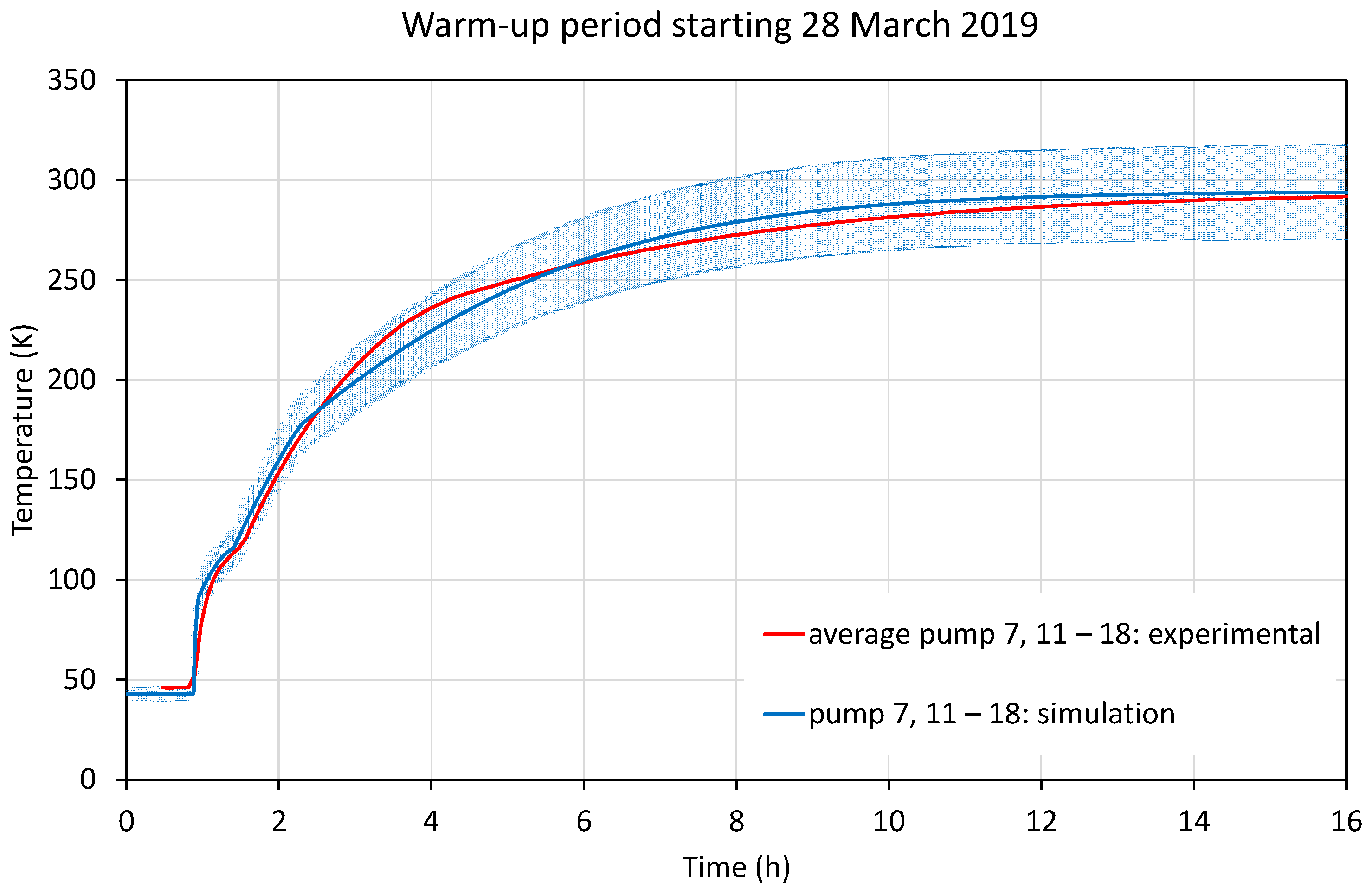
8.3. Modelling Warm-Up

The investigation of warm-up behavior uses the regeneration/warm-up cycle data shown in Figure 8, also as averages for each plate size (small round, medium square, large round), and the results are plotted in Figure 24 (small), Figure 25 (square), and Figure 26 (large). Again, the error bands are attached as shaded areas to the simulation curves.

Firstly, the modelling of the xenon sublimation inflection point is discussed. The optical model was applied to determine approximate infrared emissivity from the known approximate initial xenon layer thickness, as estimated from the thruster firing time and total xenon mass flow. The thermal part of the model was used to model the thermal gradient through the ice layer. This was necessary, since at high temperatures, due to low thermal conductivity, surface temperatures could differ from the base temperatures of the pumps. Since sublimation is determined by the ice surface temperature and is very sensitive to differences of even only a few K, the approximate surface temperature cannot just be approximated as pump temperature.

If the xenon temperature gradient data are fed into the pump heating model, the xenon peak can be well reproduced for a thickness of about 0.5mm, as shown in Figure 24, Figure 25 and Figure 26 at around 80–90 K. This corresponds to 50 sccm xenon mass flow over the course of the previously completed thruster firing. It can be seen that there are still remaining deviations, likely due to the very simplistic sublimation and thermal models, and due to the uncertainty in the initial xenon thickness.

The main observation is that this predicts a bend occurring at around 175 K, which slows down the warm-up compared with real data. This feature is present for all plate sizes.

For a more accurate shape resolution, a finite difference scheme should be used instead to properly determine the surface temperature. This will, however, cause a significant increase in the resources required for the run.

8.4. Modelling the Impact of Water on Warm-Up Behaviour

The same logic can be applied to modelling the impact of water during warm-up. Since the thickness feature of any xenon effect is not present in the curve bend caused by water, it is likely that the initial size of the water ice layer is much smaller. However, since this layer still deteriorates the optical properties of the pump (which can be noticed by observing the much smaller heating rates after water sublimation due to lowered emissivity), the minimum thickness of the water ice layer must be in the order of 1–20 μm. Thus, 10 μm was used as an initial estimate on water ice thickness. In Figure 24, Figure 25 and Figure 26, the water impact region is visible. The model predicts the water to evaporate completely at approximately 185 K, while the experiment shows the knee to occur at 195 K. This error in timing is observed in most of the results. It could be caused by either inaccurate water sublimation data or by other factors not corrected for in the simulation. The latter is likely the main reason since, as observed in the experimental data, the water sublimation region occurs each time at a different temperature (ranging from 150 K to 220 K). However, the change in emissivity is modelled well regardless of the sublimation timing.

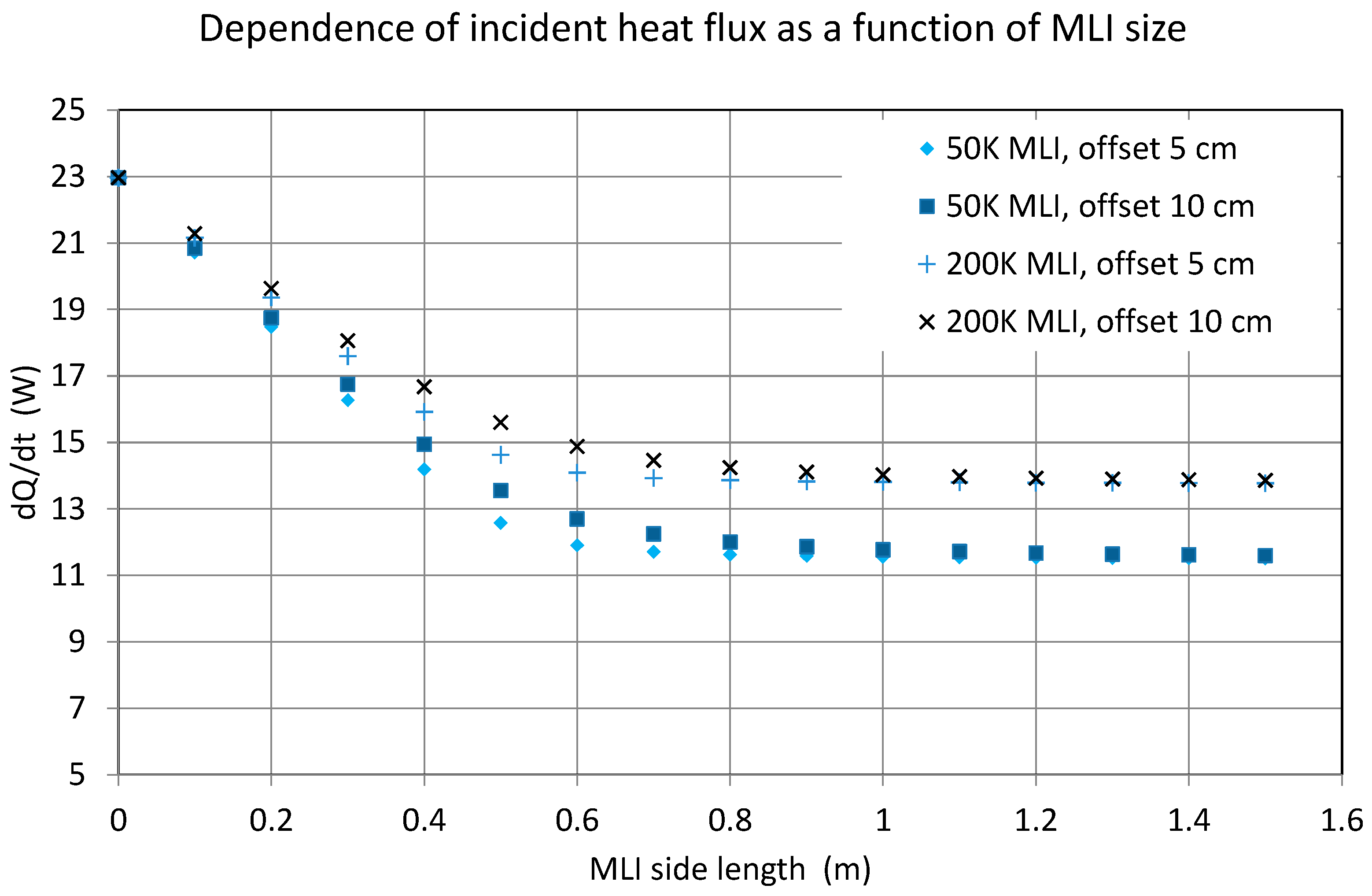
8.5. MLI Size Recommendations

Apart from the modelling of the experimental data, the software as a whole or its functions can be used to predict how design or operational parameters such as MLI size and time of water pumping (resulting in an initial water content) affect the performance of the pumps and the power budget.

As has already been shown in the section on the modelling of radiative heat transfer, the majority of the radiative heat exchange occurs due to the wall area around the underlying MLI shown in Figure 19. A cold plate of a pump has an offset of a few cm from the chamber wall, and an MLI blanket attached to the chamber screens its backside. Thus, in general, increasing this MLI area is the single most effective technique to reduce the incident heat flux. In this analysis, it is assumed that only the MLI under the pump increases in size while the sizes of the other MLIs remain the same. This assumption was made to separate the effects of these two contributions. Currently, the viewing factors of the MLI on the bottom side of the pump add up to approximately 0.94, which could be increased up to around 0.99 if a blanket of 1 m side length is used. The dependency of the heat flux on the MLI size below the pump is shown in Figure 27, which shows that choosing sizes larger than 1 m does not give better results. Furthermore, an improvement can be achieved by reducing the offset between the pump and the MLI underneath, as can be seen by comparing the offsets of 5 cm instead of 10 cm. It should be noted that these results are more of a qualitative nature and more accurate optical data and pump performance specifications would be helpful.

9. Conclusions and Outlook

Cryopumps are essential for electric space propulsion testing in ground-based facilities. The pump system of DLR’s EP Test Facility, STG-ET, with its 18 open plate cryopumps is shown in detail. These pumps provide, for the commonly used xenon gas, a pumping speed of 276 m³/s. Cryopump operation for high power thrusters is expensive, and an optimization of size and geometry is needed for the actual system and for future upgrades. For such optimizations or upgrades, a model was built in order to be able to simulate the process of cool-down, warm-up, condensation, and sublimation, with its coupled changes in surface emissivity. The model was able to reproduce fairly well the operational temperature rise due to emissivity change and the cold plate warm-up with its typical inflection regions caused by sublimation.

The deposits on the pump surfaces may contain water, and this can cause issues with respect to radiation absorption. This effect should be kept in mind when thinking about thruster technologies based on water as a green propellant.

The presented model includes MLI foils underneath the cold plate and calculates view factors. The sizes of these MLI sheets have a noticeable impact on the collected heat flux, and therefore larger sheets up to a side length of about 1 m improve performance.

Further applications of the model will help in upgrading the facility pumping system, e.g., pump location with respect to chamber inventory, like thruster and sources of sputter material, and cold plate size.

References

1. Brophy, J.R. Perspectives on the success of electric propulsion. J. Electr. Propuls. 2022, 1, 9. [Google Scholar] [CrossRef]
2. Dankanich, J.W.; Woodcock, G.R. Electric Propulsion Performance from Geo-transfer to Geosynchronous Orbits. Paper IEPC-2007-287. In Proceedings of the 30th International Electric Propulsion Conference, Florence, Italy, 17–20 September 2007. [Google Scholar]
3. Kreiner, K. The future of satellite propulsion. In Proceedings of the Presentation, EUCASS 2013, 5th European Conference for Aeronautics and Space Sciences, Munich, Germany, 1–5 July 2013. [Google Scholar]
4. Biagioni, L.; Kim, V.; Nicolini, D.; Semenkin, A.V.; Wallace, N.C. Basic Issues in Electric Propulsion Testing and the Nees for International Standards. In Proceedings of the IEPC Paper IEPC-03-230, 28th International Electric Propulsion, Toulouse, France, 17–21 March 2003; Available online: https://electricrocket.org/IEPC/0230-0303iepc-full.pdf (accessed on 15 January 2024).
5. Neumann, A.; Hannemann, K. Electric propulsion testing at DLR Göttingen: Facility and diagnostics. In Proceedings of the Presentation, Space Propulsion Conference 2014, Cologne, Germany, 19–22 May 2014. Paper Identification Number 2970582. [Google Scholar]
6. Manzella, D.; Sarmiento, C.; Sankovic, J.; Haag, T. Performance Evaluation of the SPT-140; Report NASA/TM-97-206301 NASA Center for Aerospace Information: Linthicum Heights, MD, USA, 1997. [Google Scholar]
7. Jovel, D.R.; Walker, M.L.R.; Herman, D. Review of High-Power Electrostatic and Electrothermal Electric Propulsion. J. Propuls. Power 2022, 38, 1051–1081. [Google Scholar] [CrossRef]
8. Fazio, N.; Gabriel, S.B.; Golosnoy, I.O. Alternative propellants for gridded ion engines. In Proceedings of the Paper SP2018_00102, Space Propulsion Conference 2018, Seville, Spain, 14–18 May 2018. [Google Scholar]
9. Viges, E.A.; Jorns, B.A.; Gallimore, A.D.; Sheehan, J.P. University of Michigan’s Upgraded Large Vacuum Test Facility. In Proceedings of the Paper IEPC-2019-653, 36th International Electric Propulsion Conference, Vienna, Austria, 15–20 September 2019. [Google Scholar]
10. Neumann, A. STG-ET: DLR Electric Propulsion Test Facility. J. Large-Scale Res. Facil. 2018, 4, A134. [Google Scholar] [CrossRef]
11. Goebel, D.M.; Katz, I. Fundamentals of Electric Propulsion: Ion and Hall Thrusters; JPL Space Science and Technology Series; John Wiley & Sons, Inc.: Hoboken, NJ, USA, 2008; ISBN 9780470429273. [Google Scholar]
12. Doerner, R.; White, D.; Goebel, D.M. Sputtering Yield Measurements during Low Energy Xenon Plasma Bombardment. J. Appl. Phys. 2003, 93, 5816–5823. [Google Scholar] [CrossRef]
13. Specs. Useful Information and Facts about Practice of Sputtering. Technical Report, Specs. 2023. Available online: https://www.specs-group.com/fileadmin/user_upload/products/technical-note/sputter-info.pdf (accessed on 15 January 2024).
14. Lausberg, S. Vacuum challenges for ion thruster testing. In Proceedings of the Presentation, Space Propulsion 2018, Seville, Spain, 14–18 May 2018. [Google Scholar]
15. Garner, C.E.; Polk, J.R.; Brophy, J.R.; Goodfellow, K. Methods for Cryopumping Xenon; AIAA Paper 96-3206; American Institute of Aeronautics and Astronautics, Inc.: Reston, VA, USA, 1996. [Google Scholar]
16. Kohler, M.; Frick, U. Kryopumpen in der Weltraumforschung; German Flyer; HSR AG: Balzers, Liechtenstein, 2007. [Google Scholar]
17. Neumann, A. Update on Diagnostics for DLR‘s Electric Propulsion Test Facility. Procedia Eng. 2017, 185, 47–52. Available online: www.sciencedirect.com (accessed on 15 January 2024). [CrossRef]
18. Dankanich, J.W.; Walker, M.; Swiatek, M.W.; Yim, J.T. Recommended practice for pressure measurement and calculation of effective pumping speed in electric propulsion testing. J. Propuls. Power 2017, 33, 668–680. [Google Scholar] [CrossRef]
19. Basics of Cryopumping. SHI Cryogenics Group. 2020. Available online: https://www.shicryogenics.com/wp-content/uploads/2020/09/Basics-of-Cryopumping-Booklet-English-4.18.pdf (accessed on 5 January 2024).
20. Barnes, C. Cryopumping. In Proceedings of the 1968 Summer Study on Superconducting Devices and Accelerators, Brookhaven National Laboratory, Upton, NY, USA, 10 June–19 July 1968; p. 230. [Google Scholar]
21. Perinić, G.; Vandoni, G.; Niinikoski, T. Introduction to Cryogenic Engineering. Presentation CERN, 5.-9.12.2005. Available online: https://www.slac.stanford.edu/econf/C0605091/present/CERN.PDF (accessed on 10 January 2024).
22. Thomas, J.; Peterson, J.G.; Weisend, I.I. Cryogenic Safety; Springer: Cham, Switzerland, 2019; ISBN 978-3-030-16508-6. [Google Scholar] [CrossRef]
23. Kitamura, S.; Miyazaki, K.; Hayakawa, Y.; Nakamura, Y. Xenon Ion Thruster Test Facility–Design and Operation; Paper IEPC1988-60; IEPC: Genève, Switzerland, 1988. [Google Scholar]
24. Spektor, R. Analytical Pumping Speed Models for Electric Propulsion Vacuum Facilities. J. Propuls. Power 2021, 37, 391–399. [Google Scholar] [CrossRef]
25. Marquardt, E.D.; Le, J.P.; Radebaugh, R. Cryogenic Material Properties Database. In Cryocoolers 11; Ross, R.G., Ed.; Springer: Boston, MA, USA, 2002. [Google Scholar] [CrossRef]
26. Simon, N.J.; Drexler, E.S.; Reed, R.P. Properties of Copper and Copper Alloys at Cryogenic Temperatures; Final Report; Materials Science and Engineering Laboratory, National Institute of Standards and Technology: Boulder, CO, USA, 1992. [Google Scholar]
27. Arblaster, J.W. Thermodynamic properties of copper. J. Phase Equilibria Diffus. 2015, 36, 422–444. [Google Scholar] [CrossRef]
28. Haynes, W.M.; Lide, D.R.; Bruno, T.J. CRC Handbook of Chemistry and Physics: A Ready-Reference Book of Chemical and Physical Data, 97th ed.; CRC Press: Boca Raton, FL, USA, 2016–2017; Section 6. [Google Scholar]
29. Poling, B.E.; Prausnitz, J.M.; O’Connell, J.P. Properties of Gases and Liquids, 5th ed.; McGraw-Hill Education: New York, NY, USA, 2001; Available online: https://www.accessengineeringlibrary.com/content/book/9780070116825 (accessed on 15 January 2024).
30. Tsujimoto, S.; Konishi, A.; Kunitomo, T. Optical constants and thermal radiative properties of H2O cryodeposits. Cryogenics 1982, 22, 603–607. [Google Scholar] [CrossRef]
31. Pepper, S.V. Absorption of Infrared Radiation by Ice Cryodeposits; NASA TN D5181; National Aeronautics and Space Administration: Washington, DC, USA, 1969. [Google Scholar]
32. Liu, C.K. Degradation of Cold Optical Systems by Cryodeposition; Report for 1971 Independent Research Program, AD-756 772; Lockheed Missiles and Space Company: Palo Alto, CA, USA, 1972. [Google Scholar]
33. Ferreira, A.G.M.; Lobo, L.Q. The sublimation of argon, krypton, and xenon. J. Chem. Thermodyn. 2008, 40, 1621–1626. [Google Scholar] [CrossRef]
34. Packard, J.R.; Swenson, C.A. An experimental equation of state for solid xenon. J. Phys. Chem. Solids 1963, 24, 1405–1418. [Google Scholar] [CrossRef]
Figure 1. DLR STG-ET facility with view onto cryopump cold plates with MLI foil on their backside, and beam dump targets at the end of the chamber.
Aerospace 11 00177 g001
Figure 3. Schematic diagram of pumping systems at DLR STG-ET facility.
Aerospace 11 00177 g003
Figure 4. Cold gas pumping test for xenon. The pressure is nitrogen-calibrated and not corrected for xenon (see text).
Aerospace 11 00177 g004
Figure 5. Cold gas pumping test for krypton (not gas-corrected, see text).
Aerospace 11 00177 g005
Figure 6. Cold gas pumping test for argon (not gas-corrected, see text).
Aerospace 11 00177 g006
Figure 7. Cryopump operation over 12 days. After cool-down, the cold plates reached 20–30 K. They slowly warmed up during operation.
Aerospace 11 00177 g007
Figure 8. Warm-up cycle after pump switch-off. Depending on temperature, gases sublimate and modify the temperature curves.
Aerospace 11 00177 g008
Figure 9. Schematic power curve for a Leybold cryopump CP-140T. The pump can dump about 220–230 W of heat at room temperature, and cool down to about 15–20 K (from CoolVac CP140T datasheet, Leybold GmbH).
Aerospace 11 00177 g009
Figure 10. Thermal conductivity versus temperature for copper of different purities, expressed by the RRR factor of 10–2000, see text.
Aerospace 11 00177 g010
Figure 11. Specific heat capacity of copper versus temperature.
Aerospace 11 00177 g011
Figure 12. Water ice optical emissivity versus layer thickness and material structure, from [30].
Aerospace 11 00177 g012
Figure 13. Water optical absorptance curve as compiled for the model.
Aerospace 11 00177 g013
Figure 14. Comparison of normalized ice absorptivity as a function of normalized ice layer thickness.
Aerospace 11 00177 g014
Figure 15. Xenon ice density at low temperatures.
Aerospace 11 00177 g015
Figure 16. Xenon ice-specific heat at low temperatures.
Aerospace 11 00177 g016
Figure 17. Xenon ice thermal conductivity at low temperatures.
Aerospace 11 00177 g017
Figure 18. Xenon sublimation enthalpy at low temperatures.
Aerospace 11 00177 g018
Figure 19. Basic processes of cryopump attached to a vacuum chamber. The cold plate freezes and traps the gases, and is exposed to thermal radiation from chamber walls and inner components (red arrows indicate energy flow into cryopump, blue arrows indicate energy loss from cryopump).
Aerospace 11 00177 g019
Figure 20. Flow chart of the numerical cryopump model, with the following: OPER = model of cryopumps in operation. HEAT = model of pumps warming up. t = time since beginning of pumping. tmax = maximum simulation time. T_cryo = temperature of a given cryopump. Eps_cryo = emissivity of a given cryopump. Xe_thickness = thickness of xenon layer. H2O_thickness = thickness of water ice layer. Q_rad = radiative heat flux. Xe_mdot = massflow of xenon onto pumps. Q_Xe = heat flux due to Xe adsorption/sublimation.
Aerospace 11 00177 g020
Figure 21. Comparison of data and simulation model for the cryopumps with small plates (pumps 1–6) during operation after cool-down during 10 operational days with applied xenon mass flow (see Section 4 for pump specifications). The shaded area is the simulation error, see text.
Aerospace 11 00177 g021
Figure 22. Comparison of data and simulation model for the cryopumps with rectangular plates (pumps 8–10, see Section 4 for pump specifications). The shaded area is the simulation error, see text.
Aerospace 11 00177 g022
Figure 23. Comparison of data and simulation model for the cryopumps with large round plates (pumps 7, and 11–18, see Section 4 for pump specifications). The shaded area is the simulation error, see text.
Aerospace 11 00177 g023
Figure 24. Comparison of warm-up data and model for the small cryopumps after pump switch-off on 28 March 2019. Warming up releases xenon and produces the inflection point in the 60–110 K range. The second inflection point, more pronounced in the simulation curve, comes from water sublimation. The shaded area is the simulation error, see text.
Aerospace 11 00177 g024
Figure 25. Comparison of warm-up data and model for the cryopumps with square plates after pump switch-off (see legend of Figure 24).
Aerospace 11 00177 g025
Figure 26. Comparison of warm-up data and model for the large plate cryopumps after pump switch-off (see legend of Figure 24).
Aerospace 11 00177 g026
Figure 27. Effect of MLI area on received heat of the pump above it, for 10 cm and 5 cm distance offset between cold plate and chamber wall.
Aerospace 11 00177 g027