Article

Stacked Multiscale Densely Connected Temporal Convolutional Attention Network for Multi-Objective Speech Enhancement in an Airborne Environment

School of Power and Energy, Northwestern Polytechnical University, Xi’an 710072, China
*
Author to whom correspondence should be addressed.
Aerospace 2024, 11(2), 156; https://doi.org/10.3390/aerospace11020156
Submission received: 9 December 2023 / Revised: 6 February 2024 / Accepted: 7 February 2024 / Published: 15 February 2024

Abstract

:
Airborne speech enhancement is always a major challenge for the security of airborne systems. Recently, multi-objective learning technology has become one of the mainstream methods of monaural speech enhancement. In this paper, we propose a novel multi-objective method for airborne speech enhancement, called the stacked multiscale densely connected temporal convolutional attention network (SMDTANet). More specifically, the core of SMDTANet includes three parts, namely a stacked multiscale feature extractor, a triple-attention-based temporal convolutional neural network (TA-TCNN), and a densely connected prediction module. The stacked multiscale feature extractor is leveraged to capture comprehensive feature information from noisy log-power spectra (LPS) inputs. Then, the TA-TCNN adopts a combination of these multiscale features and noisy amplitude modulation spectrogram (AMS) features as inputs to improve its powerful temporal modeling capability. In TA-TCNN, we integrate the advantages of channel attention, spatial attention, and T-F attention to design a novel triple-attention module, which can guide the network to suppress irrelevant information and emphasize informative features of different views. The densely connected prediction module is used to reliably control the flow of the information to provide an accurate estimation of clean LPS and the ideal ratio mask (IRM). Moreover, a new joint-weighted (JW) loss function is constructed to further improve the performance without adding to the model complexity. Extensive experiments on real-world airborne conditions show that our SMDTANet can obtain an on-par or better performance compared to other reference methods in terms of all the objective metrics of speech quality and intelligibility.

1. Introduction

Noise contamination is all around us. For instance, environmental noise in daily life may heavily affect the usage of modern telecommunication devices or hearing aids. Recently, in the aviation field, airborne noise has significantly impaired communication between the cabin and ground personnel, which has attracted the attention of many researchers. To tackle this problem, monaural speech enhancement is proposed to separate background noise from noisy input signals and improve the quality of utterances. Many classical algorithms, such as spectral subtraction [1], Wiener filtering [2], and statistical methods [3], have been extensively studied in recent decades. These methods are usually only able to handle stationary noise but lack the ability to suppress non-stationary noise interference.
Thanks to the rapid expansion of deep neural networks (DNNs), deep-learning-based speech enhancement methods have shown great superiority in dealing with most non-stationary noise cases [4,5,6]. In these data-driven methods, the speech enhancement task is formulated as a supervised learning problem focusing on time–frequency (T-F) masking [7,8] or speech spectral mapping [9,10]. Apparently, existing deep-learning-based enhancement methods can be divided into two categories, namely single-objective learning and multi-objective learning (MOL), according to the numbers and types of targets being learned simultaneously. Previous studies have shown that multi-objective learning generally yields a better noise reduction performance than single-objective-based learning [11]. In short, the joint training of different but complementary targets can potentially achieve better speech quality and intelligibility. In a typical MOL-based speech enhancement system, the log-power spectra (LPS) or amplitude modulation spectrogram (AMS) often acts as a representative spectral mapping-based target [12,13]. The frequently used T-F domain learning target is the ideal ratio mask (IRM), which is strongly complementary to LPS in boosting speech enhancement performance [14].
Advanced MOL-based speech enhancement technologies depend on a strong and effective network architecture. Early researchers employed the unsophisticated multi-layer perception (MLP) structure to simultaneously predict the clean spectral features and IRM, which removed noise interference to a certain extent [15,16]. However, the complete connection structure of MLPs cannot capture the long-range acoustic feature information of the speech frames, which undoubtedly makes modeling more sophisticated interactions difficult. To address this issue, recurrent neural networks (RNNs) and deep convolutional neural networks (CNNs) have been introduced into speech enhancement, achieving remarkable performance improvements. In [17], an RNN with four long short-term memory (LSTM) layers was proposed to model the long-term contextual information of a given utterance, which yielded more effective noise reduction than an MLP. Subsequently, Gao et al. [18] adopted an LSTM as a sequence-to-sequence regression function to perform MOL-based speech enhancement. Even though the work in [18] successfully outscored the standard regression method, its enhanced performance is still limited by its large space complexity. It is generally known that a CNN typically has fewer trainable parameters than an MLP and an RNN owing to its weight-sharing property. Therefore, a temporal convolutional neural network (TCNN) was proposed in [19], which would consume fewer parameters when modeling long-term dependencies of the speech spectrum. The TCNN, utilizing causal and dilated kernels, demonstrated substantial performance improvements compared to the above networks for temporal modeling tasks. Inspired by the success of the TCNN, in [20], Li et al. proposed a stacked and temporal convolutional neural network (STCNN) to jointly implement the spectrum mapping and T-F masking tasks. The STCNN benefited immensely from the feature extraction ability of the stacking CNNs (SCNNs) and the temporal modeling ability of the TCNN, and, as a result, has a state-of-the-art performance in the MOL-based speech enhancement field.
In addition to the network model, the loss function is also crucial for multi-objective speech enhancement algorithms. In earlier studies [9,10,11,12], a well-established way of indicating the direction of the network model optimization is minimizing the mean-square error (MSE) between the predicted results and target spectral representations (e.g., the target oracle LPS or IRM), which gained some success in multi-task learning. Notably, when applied in the mask estimation task, this objective function is also noted as the mask approximation (MA) loss [21]. However, this commonly seen MA function is not directly optimized for the actual speech spectral target, which may lead to the whole system reconstructing the spectrogram of clean speech inaccurately in the post-processing stage. To compensate for this inadequacy, recent studies [21,22] proposed a mask-based signal approximation (MSA) loss function to perform a mask estimation task. By using MSA, a network model can be employed to estimate the IRM but can be also trained to minimize the MSE between the clean speech spectrum and the enhanced spectrum reconstructed by the estimated IRM. In this way, the masking-based enhancement approach achieves an improved performance with the same inference complexity as before. Furthermore, this study also reveals that combining the MA and MSA functions to optimize the mask estimation task can further improve the quality of enhancement. However, the previous works shown in [21] only use a simple, average way of combining MA and MSA, which cannot fully utilize the influence of MA and MSA on the performance of the masking-based speech enhancement task.
On the whole, despite the merits of the existing advanced multi-objective speech enhancement methods, such as the STCNN in [20], they still have possible limitations in jointly optimizing the complicated regression between the contaminated input feature and the ideal LPS and IRM target, especially under unexpected noise scenarios. First, in the STCNN, the extracted feature maps generally have the same receptive field size. In general, such a single-scale fixed-size feature map cannot well reflect the complex acoustic structures of the speech signal, which may hinder the network in learning high-level acoustic characteristics hidden in the target data. Second, due to its limited representations of the training utterances, some networks with less attention (e.g., TCNN or STCNN) usually have poor sensitivity to the informative features that will undoubtedly damage the temporal modeling performance of weak speech components. Third, the whole STCNN only simply uses the single-forward traditional connection manner, namely passing the features from one layer to the next layer, which may suppress the information flow of the network. Finally, the STCNN adopts the basic MSE criterion between the output and the corresponding learning target as the loss function, which does not directly reflect the actual magnitude spectrum of clean speech. According to the previous analysis, this loss function in the STCNN is not conducive to obtaining optimal performance for the masking subtask.
To tackle these problems mentioned above, in this paper, we propose a stacked multiscale densely connected temporal convolutional attention network (SMDTANet) for multi-objective speech enhancement in the real-world airborne noise scenario. Specifically, the proposed SMDTANet introduces three novel modules, namely a stacked multiscale feature extraction module, a triple-attention-based TCNN (TA-TCNN), and a densely connected prediction module, as the main components to achieve a state-of-the-art multi-objective speech enhancement performance. First, the input noisy LPS are applied to the stacked multiscale feature extractor for the learning of the characteristics of different time scales. Then, the additional mixture AMS feature is used as the secondary input, combined with the output of our feature extractor, that is fed into the TA-TCNN for temporal sequence modeling. Finally, the final LPS and IRM outputs are estimated by using the densely connected prediction module. Moreover, our SMDTANet is trained using a new joint-weighted (JW) loss function in the whole learning process. The core contributions of this paper are summarized as follows:
  • A stacked multiscale feature extractor is proposed to improve the abstract feature extraction ability. By stacking multiple multiscale blocks, our feature extractor can garner much larger receptive fields and provide discriminative information of different scales for obtaining better speech enhancement performance.
  • A triple-attention block is designed to optimize the TCNN, enabling it to focus simultaneously on regions of interest in the channel, spatial, and T-F dimensions, thereby enhancing its ability to model the temporal dependencies of speech signals.
  • Constructed with two dense connection convolution blocks, a densely connected prediction module is built which can strengthen feature propagations and enhance the information flow of the network to produce a more robust enhancement performance.
  • To fully leverage the advantages of MA and MSA loss functions for learning mask targets, a new joint-weighted loss function is proposed, which can make SMDTANet optimize the masking subtask in both the TF magnitude and masking domains simultaneously.
Extensive experiments were conducted using real-world airborne noise data and commonly used ambient noise data. The results show that our SMDTANet can obtain superior enhancement performance compared to the reference methods in unseen noise conditions, especially in the unseen airborne noise condition.
The remainder of this paper is organized as follows: In Section 2, we briefly describe the traditional multi-objective speech enhancement framework and the baseline STCNN structure as preliminaries. The components and structure of the proposed SMDTANet network are introduced in Section 3. Section 4 and Section 5 present the experimental setup and the performance evaluation, respectively. Finally, we summarize this paper in Section 6.

2. Related Work

2.1. Multi-Objective Speech Enhancement

In monaural speech enhancement, a noisy mixture signal can be modeled in the time–frequency (T-F) domain as
Y ( t , f ) = X ( t , f ) + N ( t , f )
where X ( t , f ) , N ( t , f ) , and Y ( t , f ) denote the short-time Fourier transform (STFT) values of the clean speech, the additive noise, and the mixed speech, respectively. And t and f correspond to the time frame and the frequency index. The goal of the monaural speech enhancement task is to obtain the best estimate of clean speech from a noisy spectral feature. Motivated by the boosting concept [11], multi-objective learning technology is employed to perform this speech spectrum estimate task. In the MOL-based speech enhancement system, multiple auxiliary acoustic features are utilized as inputs to the speech enhancement network to concurrently estimate the multiple learning targets.
Generally speaking, LPS or AMS is one of the commonly used features of speech enhancement. These features are concatenated as the input layer of the MOL-based speech enhancement model. Similar to the concept of auxiliary inputs, the output layer of the MOL-based model typically employs two types of learning targets: clean LPS and IRM. The LPS target can be obtained by a logarithmic compression operation:
z L P S ( t , f ) = log | X ( t , f ) | 2
The IRM can explicitly provide the speech-dominant or noise-dominant information of each T-F unit, the definition of which can be presented as follows:
z I R M ( t , f ) = X 2 ( t , f ) X 2 ( t , f ) + N 2 ( t , f )
Then, the training process using a multi-objective MSE criterion can be expressed as
E 1 = 1 T t = 1 T f = 1 F [ z ^ L P S ( t , f ) z L P S ( t , f ) 2 2 + z ^ I R M ( t , f ) z I R M ( t , f ) 2 2 ]
where z L P S ( t , f ) and z I R M ( t , f ) are the ideal LPS and IRM features; z ^ L P S ( t , f ) and z ^ I R M ( t , f ) are the clean estimations of the above-mentioned features. T and F are the sizes in the time and frequency axes, respectively. Finally, the estimated LPS and IRM features of this system are averaged to reconstruct the speech spectrum:
X ^ ( t , f ) = 1 2 { z ^ L P S ( t , f ) + [ Y L P S ( t , f ) + ln z ^ I R M ( t , f ) ] }
where Y L P S ( t , f ) denotes the noisy LPS features. The reconstructed spectrum in a ( t , f ) t h unit is then used with the noisy phase to obtain the time domain waveform of the enhanced speech.

2.2. Baseline STCNN Network Topology

In general, the performance of the network plays an essential role in the MOL-based speech enhancement system. To achieve satisfactory speech enhancement performance, Li et al. [20] have developed an STCNN framework that has been successfully applied to learn the mapping relationship between the noisy multi-stream features and the ideal complementary targets. Figure 1 shows the STCNN architecture in [20] for the multi-objective speech enhancement task. It comprises two important modules: a stacked CNN structure with local connection characteristics and a recently popularized TCNN with a strong temporal modeling capacity. The SCNN is a typical stacked convolutional structure that is employed to capture complex local features of the log-power spectral domain. Another module (TCNN) combining causal and dilated convolutional layers is used as a better temporal hierarchy to provide long-term historical information for the sequence modeling of the speech signal.
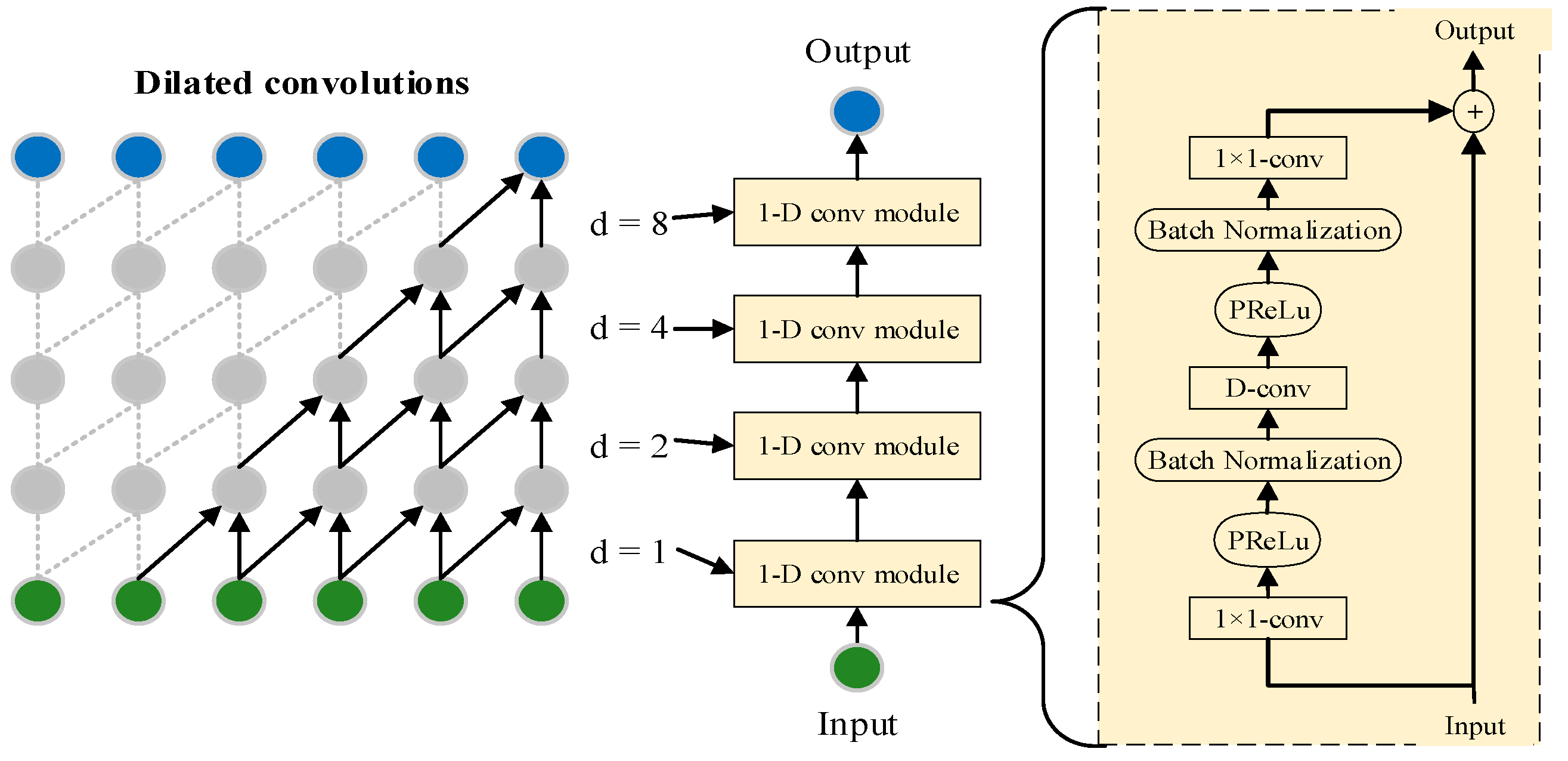
Specifically, as shown in Figure 1, the SCNN is constituted in order by a 3 × 3 conv, a batch normalization operation, and a maximum pooling layer. Unlike a conventional CNN, as illustrated in Figure 2, the TCNN is a general convolutional network with causal and dilated convolutional layers proposed for temporal sequence modeling [19]. Given the input sequence x 0 , x t and the corresponding output sequence y 0 , y t , the predicted y ^ 0 , y ^ t sequence is generated by a sequence modeling network. The prediction y ^ t depends only on the x 0 , x t but not on the future input sequence x t + 1 , x T , which means that the TCNN is a causal constraint neural network. This causal convolutional structure can help the whole network to strengthen the time constraints. In other words, the TCNN is a one-way model that can ensure no information leakage from the future to the past. And the dilated convolutions in the TCNN are introduced to expand the length of causal convolution sequence modeling. As shown in Figure 2, the dilated causal convolution slides over inputs by skipping values with a fixed step. Mathematically, the output of the dilated convolution F d ( t ) can be defined as
F d ( t ) = ( x f d ) = i = 0 K 1 f d ( i ) x ( t d i )
where f d and K denote the dilated convolution kernel and its kernel size, respectively. d is the dilation factor, and x ( t d i ) represents the past frames for analysis. In the TCNN, d is usually increased exponentially (i.e., 1, 2, 4, 8, 16, and 32) to ensure a large time context window to extract the long-range dependence of the speech signal. Because the dilation range grows exponentially, stacked dilated convolution can provide a larger receptive field for the whole network, which allows the TCNN to capture the temporal dependence of various resolutions with input sequences.
Additionally, as shown in the dotted box in Figure 2, the TCNN also adopts residual connection to accelerate learning and mitigate the gradient explosion problem. Each residual block in the TCNN comprises three layers of 1 × 1 convolutions (1 × 1 Conv): input 1 × 1 Conv, depth-wise convolution (D-conv), and output 1 × 1 Conv. The input 1 × 1 Conv is exploited to double the number of incoming channels. The middle D-conv layer is used to control the number of trainable parameters. The output 1 × 1 Conv layer returns the original number of channels, which can ensure the dimensions of the input and the output layer are consistent. Apart from the final convolution layer, each convolution layer is followed by a rectifying linear unit (ReLU) and a batch normalization operation.
On the whole, this STCNN-based multi-objective speech enhancement system consists of three major processing stages: the feature extractor (SCNN), the TCNN module for temporal sequence modeling of speech signals, and the separation module (two fully connected layers). First, noisy LPS features are fed into stack convolutional layers, and then the outputs of the SCNN, concatenated with other auxiliary acoustic features, are given as the input of the TCNN module. Finally, the two purely feed-forward layers return an estimate of the clean LPS and IRM.

3. Proposed System Description

On the basis of the STCNN architecture in [20], a stacked multiscale densely connected temporal convolutional attention network (SMDTANet) is proposed in this paper for multi-objective airborne speech enhancement. The SMDTANet has extended the network structure and training loss function of the baseline STCNN framework to better perform spectral mapping and mask estimation simultaneously. For its architecture, we first propose a stacked multiscale extractor instead of the SCNN extractor to capture higher-level abstract information from the input feature maps. Then, we design a new triple-attention module and incorporate it into TCNN to emphasize more critical and discriminative details of the multiscale information. Finally, we introduce dense blocks to process all information to guide the final target prediction. Moreover, we propose a new weighted loss function to further accelerate learning and boost speech enhancement performance in the airborne environment.
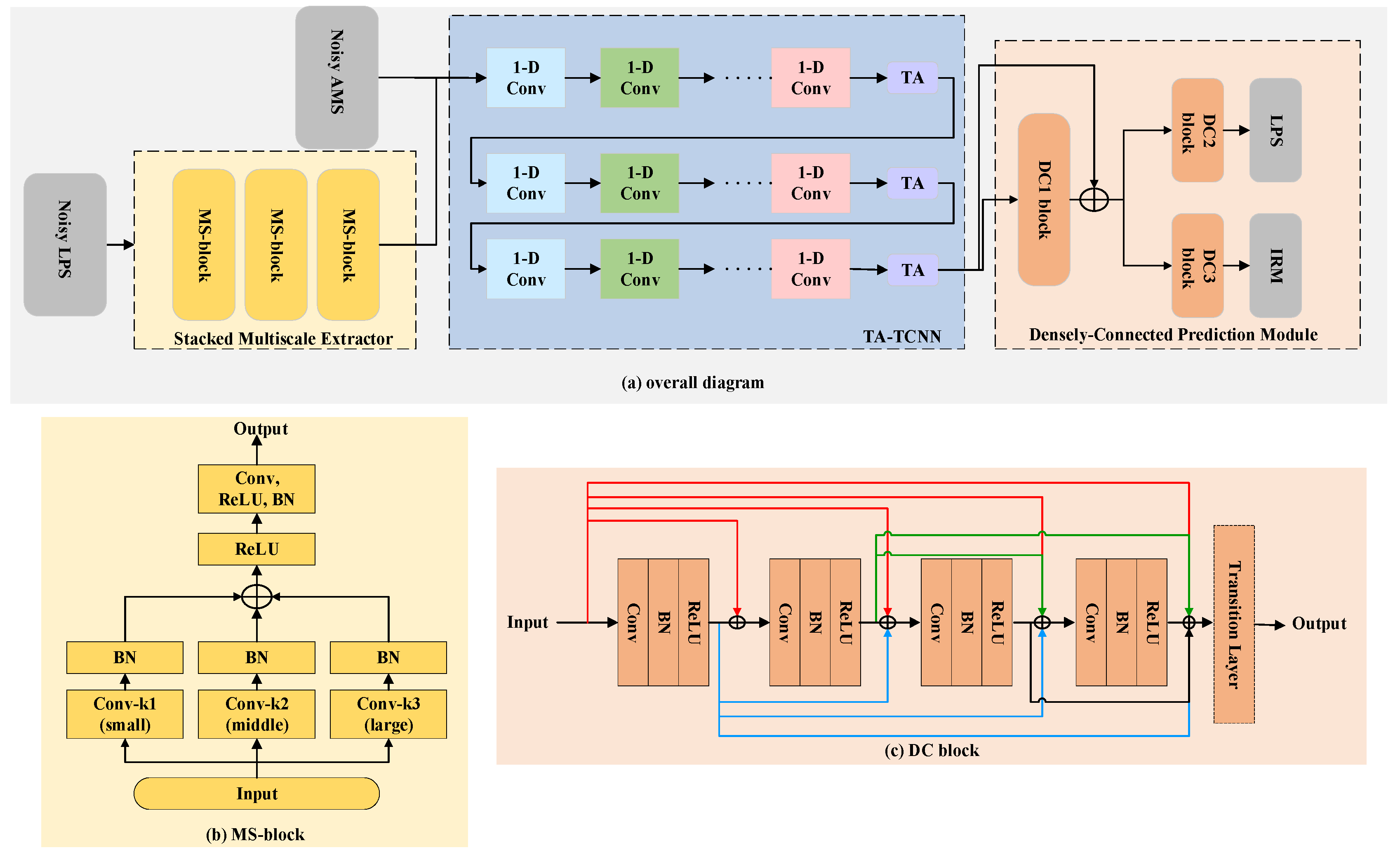
Figure 3 illustrates the flowchart of the proposed SMDTANet. The core of this network consists of three parts, namely a stacked multiscale feature extractor, a TA-TCNN, and a densely connected prediction module. Specifically, the stacked multiscale feature extractor adopts the noisy LPS vectors ( Y L P S R T × F × 1 ) as input to capture implicit high-level acoustic information from multiple time scales. Then, the outputs of this feature extractor, combined with auxiliary noisy AMS vectors ( Y A M S R T × F × 1 ), are fed into the TA-TCNN to perform sequence-to-sequence modeling. Finally, the densely connected prediction module is used as a preferred output layer to return the estimated LPS ( z ^ L P S R T × F × 1 ) and IRM ( z ^ I R M R T × F × 1 ). Now, we will gradually show more details of the proposed SMDTANet network and each network module.

3.1. Stacked Multiscale Feature Extraction

Many speech enhancement algorithms tend to use a single-scale convolution module (e.g., the reviewed SCNN in Section 2.2) to capture local features of speech and implicit correlations in the T-F domain for the final mask prediction or spectral mapping. Generally, in such a simplified single-scale feature extractor, the conventional convolution within a fixed receptive field can perform well in capturing the protruding structure of the voice signal, which will contribute to reducing background interference to a certain extent. However, non-periodic acoustic elements in the clean speech data, such as successive consonants, aspirated sounds, or voiceless fricatives, usually exhibit complex spectral textures in the spectrogram. Unsurprisingly, it is hard for a single-scale convolution module to extract those high-level textures due to its own fixed-size receptive field. In contrast, it has been found that a multiscale module can capture more comprehensive feature information by skillfully changing convolution kernel sizes [23,24]. Moreover, stack convolution architecture can further expand the receptive field serially, which makes it better able to improve the nonlinear representation of the whole network for abstract features. Motivated by these findings, in this paper, we propose a stacked multiscale feature extractor to capture local feature information of speech on different time scales.
Specifically, as shown in the yellow dashed rectangular box in Figure 3a, our feature extractor consists of three lightweight multiscale convolution blocks (MS-blocks), in which the convolution kernel size sets of different MS-blocks vary. Details of each MS-block are illustrated in Figure 3b. Each MS-block employs three 1-D convolutional layers with different kernel sizes, denoted as k1 (small), k2 (middle), and k3 (large), respectively, to extract multiscale vocal characteristics from inputs in parallel. In detail, the sizes of the kernel set of those three MS-blocks are {1,3,5}, {3,5,7}, and {5,7,9}, respectively. Each convolution has the same number of convolutional filters as the input shape. The convolutions in the MS-block are followed by a batch-normalized layer to facilitate the network training. Thereafter, the output of the MS-block can be obtained by fusing all extracted timescale features before the rectified linear unit (ReLU) activation function is applied to it.
Let F M S 1 , F M S 2 , and F M S 3 denote the extracted features from different kernels, respectively; the process of generating the final output can be expressed as
Y M S = f M S ( δ ( A d d ( [ F M S 1 , F M S 2 , F M S 3 ] ) ) )
where δ refers to the ReLU activation function, and A d d ( ) is the additive function that can fuse features of different scales without increasing computation cost. f M S ( ) represents the combination of nonlinear mapping operations in this module, including a convolutional layer with a kernel size of 1, a rectifier nonlinearity (ReLU) activation, and a batch normalization (BN), to fuse three features into the final feature. In each MS-block, the number of filters in each convolutional layer is equal to the input shape. Finally, we stack another two MS-blocks with the various sets of kernel sizes to further provide a larger receptive field for the whole network.

3.2. Triple-Attention-Based TCNN (TA-TCNN)

As discussed earlier, the TCNN has been widely utilized as a backbone architecture for most speech enhancement networks, owing to its powerful ability to model temporal dependencies of speech signals. Although such good temporal modeling performance has been obtained by the TCNN, there is still room for further improvement. The use of an attention mechanism is a widely accepted technique that enables the network to selectively aggregate key contextual information and automatically ignore other irrelevant information. Through this selective information aggregation mechanism, the speech enhancement network can better preserve the desired speech characteristics and remove uncorrelated noise information more effectively. Currently, there are three popular ways to compute the attention vector in speech enhancement deep networks: channel attention [25], spatial attention [25], and time–frequency (T-F) attention [26]. By using different perspectives to discriminate the importance of different contextual spectral information, each way has its unique advantage in boosting network performance. For instance, previous studies [27,28] have found that channel attention can find out which channel feature information is crucial for training and thus reassign weights to feature vectors of different channels. Spatial attention usually flexibly weights feature information according to the importance of its spatial location. T-F attention is one of the recently popularized attention mechanisms; it aims to capture significant temporal and frequency-wise information simultaneously. Inspired by these successful mechanisms, in this paper, we propose a TA module to fully utilize the potentials of channel attention, spatial attention, and T-F attention for optimizing the TCNN.
As shown in the blue area of Figure 3, the TA-TCNN module adopts the combination of the third MS-block output and the noisy AMS feature as inputs. In short, the input size for TA-TCNN is T × 2 F . The TA-TCNN is constructed by three temporal convolutional groups and three triple-attention modules. To be specific, each group, including six residual convolutional blocks with exponentially increasing dilation factors 2 b ( b { 0 , , 5 } ) , is followed by a TA module. The kernel size of each temporal convolutional group is set to 3. The size of the final TA-TCNN output is the same as the input size. Except for the input and output layers, the length of other intermediate convolutional layers in TA-TCNN is 256 which is similar to the baseline TCNN in [19].
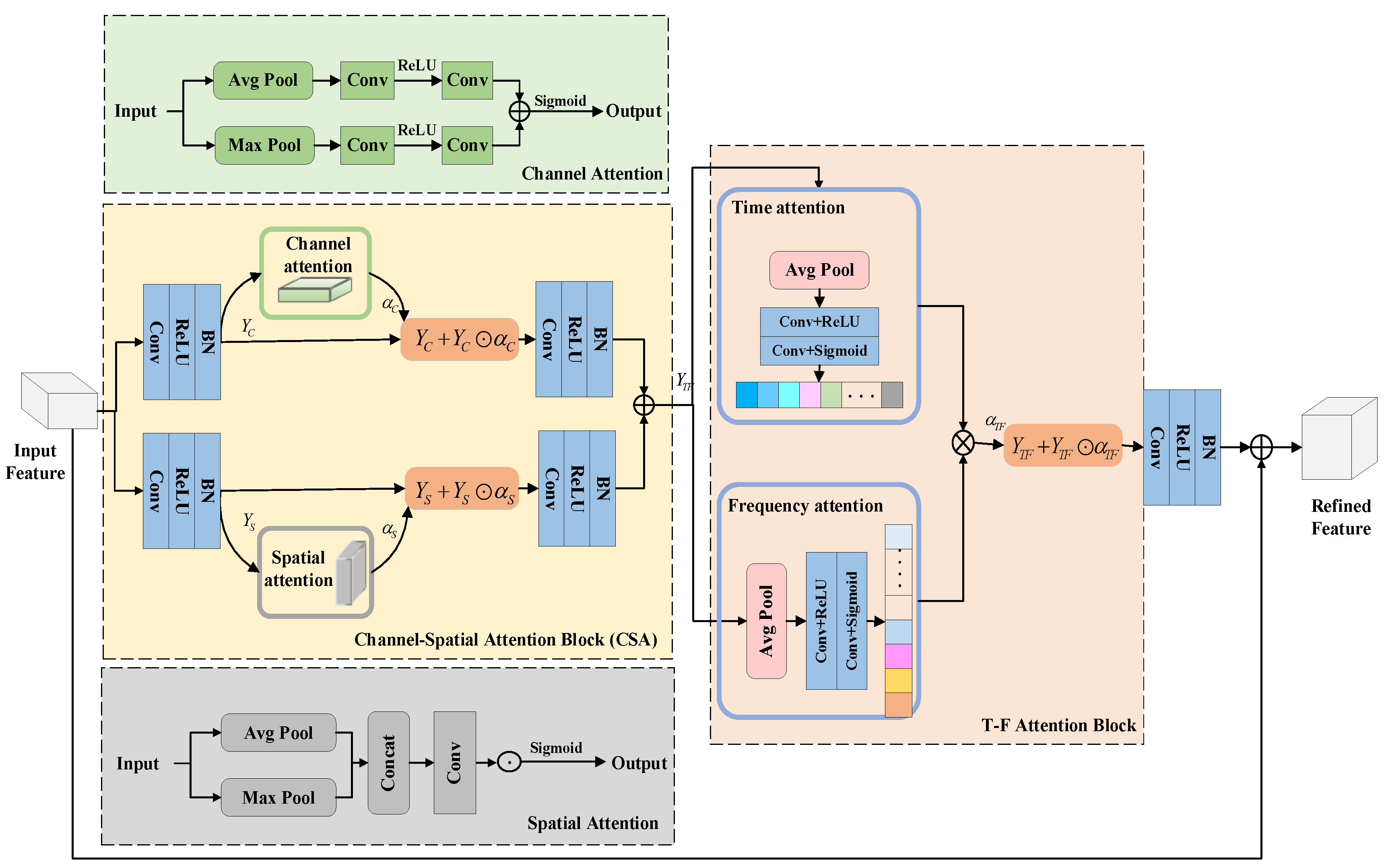
The layout of the TA module is presented in Figure 4. As shown in Figure 4, our TA module is designed by concatenating three different attention mechanisms, namely channel attention, spatial attention, and T-F attention. Our TA module can be considered a triple-region module from the perspective of attention types. To be specific, two parallel regions in the left part of Figure 4 are used to merge channel attention with spatial attention to capture components of interest in both the channel and spatial dimensions simultaneously. For brevity, in Figure 4, the two parallel routes for capturing channel and spatial representation are denoted as the “channel–spatial attention (CSA) block”. The third region, as shown in the right part of Figure 4, is the T-F attention block, which aggregates the feature maps along the time and frequency dimensions to emphasize the T-F representation of the speech signal.
Given a feature map Y T C N R T × 2 F produced by a temporal convolutional group as the input of the TA module, we first design the CSA block to capture a joint channel–spatial representation. As shown in the left part of Figure 4, in the CSA block, before the channel and spatial attention block is used, Y T C N is first subjected to a convolution operation with a size-3 kernel to enhance the nonlinear representation of the network and create a 256-dimensional feature map. To alleviate the parameter burden, we feed this low-dimensional feature into the channel and spatial attention block to obtain channel-wise and spatial representation, respectively. After obtaining the channel output Y C and the spatial output Y S , we also adopt a convolution operation of kernel size 3 to obtain their respective refined attention outputs. Then, we combine those refined outputs via element summation to generate the final CSA output F C S A :
F C S A = A d d ( [ f C S A 0 ( Y C ) , f C S A 1 ( Y S ) ] ) )
where f C S A 0 ( ) and f C S A 1 ( ) are the convolution operations applied to Y C and Y S , respectively. Finally, we pass F C S A through the T-F attention block and a convolutional layer to obtain the refined T-F representation. Moreover, the residual connection is introduced to facilitate information flow in the entire TA module. In short, the output of the TA-TCNN Y T C N is written as
Y T C N = Y T C N + f T A M ( M T F ( F C S A ) )
where M T F ( ) represents the T-F attention operation. f T A M ( ) is a convolutional operation with a kernel size of 1. Note that all convolutions used in the TA module are followed by ReLU and BN.
On the whole, in the TA module, the input features pass through the CSA block and the T-F attention block serially, and then these multi-view attention maps are fused by a convolution operation and residual connection to produce the final output features. We will describe all regions of the TA module in detail in the following subsections.

3.2.1. Channel Attention

We employ the channel attention proposed in [25] to emphasize the finer channel-wise representations. As shown in the green area of Figure 4, in a typical channel attention block, we first apply the global average-pooling and global max-pooling operations to the input feature Y C R T × d m o d e l to aggregate the channel information, where d m o d e l is the frequency-wise channel size. In this paper, d m o d e l is set to 256. Then, each pooling output is fed to two shared convolutional layers with a kernel size of 1. After these shared layers, the channel attention map α C is calculated as follows:
a C = σ ( W 1 ( W 0 ( F A v g ( Y C ) ) ) + W 1 ( W 0 ( F M a x ( Y C ) ) ) )
where σ refers to the sigmoid function. F A v g ( ) and F M a x ( ) denote the global average-pooling and global max-pooling, respectively. Note that the weights of the shared layers, W 0 and W 1 , are shared for both input vectors, and the ReLU function is followed by W 0 . Finally, the channel attention output Y C can be expressed as
Y C = Y C + Y C α C
where represents an element-wise multiplication.

3.2.2. Spatial Attention

Different from using channel attention, we adopt the spatial attention proposed in [25] to infer the latent inter-spatial relationships of features. As shown in the gray area of Figure 4, to extract spatial information, we first apply the global average-pooling and global max-pooling operation along the channel axis to Y S R T × d m o d e l , where Y S is the input of the spatial attention. After different pooling features are concatenated, a refined feature descriptor is generated and then forwarded to a standard convolution layer so that our spatial attention map can be obtained. In short, the spatial attention map α S is formulated as follows:
α S = σ ( f S A ( C a t [ F A v g ( Y S ) , F M a x ( Y S ) ] ) )
where C a t [ , , ] denotes the concatenation operation, and f S A ( ) is a convolution layer with a kernel size of 1. Let Y S stands for the input of the spatial attention block; the spatial attention output can be defined as Y S = Y S + Y S α S .

3.2.3. Time–Frequency (T-F) Attention

As mentioned earlier, in this paper, we also introduce the T-F attention presented in [26] and exploit it to characterize a salient energy distribution of speech in the time and frequency dimensions. As shown in the right part of Figure 4, the T-F attention block includes two parallel attention paths: time-dimension attention and frequency-dimension attention. The former works on the frequency axis to produce a 1-D time-frame attention feature, F T A R 1 × T , and the latter works on the time axis to obtain a 1-D frequency-dimension attention feature, F F A R d m o d e l × 1 . Specifically, the given input Y T F R T × d m o d e l is first passed through the global average-pooling layer along the frequency dimension to obtain a time-frame-wise descriptor, Z T A R 1 × T :
Z T A ( t ) = f = 1 d m o d e l Y T F ( t , f ) / d m o d e l
Then, we employ two stacked convolutions with a filter of size 1 to capture the dependence in the descriptor Z T A , resulting in the time-frame attention map F T A :
F T A = σ ( f T A 2 ( δ ( f T A 1 ( Z T A ) ) ) )
where f T A 1 and f T A 2 denote two convolutional operations used in the TA branch. Similarly, the frequency-wise descriptor Z F A R d m o d e l × 1 can be obtained by applying the global average-pooling operation along the time dimension on Y T F :
Z F A ( f ) = t = 1 T Y T F ( t , f ) / T
Then, the frequency-wise attention map F F A is computed as
F F A = σ ( f F A 2 ( δ ( f F A 1 ( Z F A ) ) ) )
Next, those two attention maps are combined via a tensor multiplication operation, resulting in the final 2-D T-F attention weight α T F as follows:
α T F ( t , f ) = F T A ( t ) F F A ( f )
where represents a tensor multiplication. Finally, the output of our T-F attention block is given as Y T F = Y T F + Y T F α T F .

3.3. Densely Connected Prediction Module

Dense connection [29,30] has been proven effective in enhancing feature map reuse, reducing interdependence between layers, and facilitating information flow in convolutional neural networks. In some sense, it can be regarded as a natural evolutionary version of the connectivity mode from the traditional network, which can provide valid information from different hierarchical layers for the final prediction. In order to estimate the clean speech spectrum or the ratio mask more accurately, in this paper, we introduce dense connectivity and propose to replace two conventional fully connected layers in the baseline STCNN with a novel densely connected prediction module as the post-processing part of the whole multi-task network. In addition, the residual connection is also added to avoid gradient vanishing or explosion in the whole network. The entire structure of our densely connected prediction module is illustrated in Figure 3c; it consists of three densely connected (DC) blocks, named DC1, DC2, and DC3, respectively. DC1 accepts the feature maps produced by previous MLA-based TCNN modules and processes them to capture multi-level feature information flow from all preceding layers. DC2 and DC3 are mainly intended to locate the key information of each subtask, which will enable our SMDTANet to respectively perform the spectral enhancement and mask estimation more accurately.
Specifically, due to using the output of TA-TCNN as the inputs, the input size for each DC block is T × 2 F . As shown in Figure 3c, each DC block is constituted by a transition layer and four dense convolutional units with nonlinear functions of 1-D Conv, BN, and ReLU. The convolution operation in each dense unit is made by a size-3 kernel. For the four dense units, the inputs of the current dense unit are generated by splicing and merging with all outputs of the preceding dense units. In this layout, different level feature information can be reused in subsequent units to improve the robustness of the SMDTANet. After using these dense convolutional operations, we employ a transition layer to effectively fuse those multi-level features for achieving better prediction. Mathematically, the output of each block ( Y D C ) can be expressed as
Y D C = f T ( A d d [ Y D C 0 , Y D C 1 , Y D C 2 , Y D C 3 , Y D C 4 ] )
where Y D C 0 is the input of this whole block, and Y D C i denotes the output at layer i. f T ( ) refers to the composite function of the transition layer in these blocks. In detail, the transition layer in DC1 comprises a basic Conv with a kernel size of 1, followed by the BN operation and a ReLU activation layer. The transition layer in DC2 or DC3 is used as a final output layer for each task, which only includes a traditional feed-forward layer with linear or sigmoid activation. Apparently, the linear function is applied to the transition layer of the DC2 block that targets the LPS, whilst a sigmoid nonlinearity is appropriate for the DC3 block which uses IRM as the learning target. In addition, except for the final output layer in DC2 or DC3, all convolution filters in those three DC blocks have the same length as the input vector. And the output layer in DC2 or DC3 has the same length as its corresponding target vector.

3.4. Joint-Weighted (JW) Loss Function

Generally speaking, as shown in Equation (4), the fundamental loss function of a multi-objective speech enhancement system is a distance metric between the output and its corresponding ground truth (e.g., the clean LPS feature or reference IRM). When using such a straightforward loss, these mask targets can be exactly minimized in the T-F masking domain, which will enable the enhancement system to yield the best mask estimation result. Another better distance metric for the masking task is a mask-based signal approximation (MSA) loss function proposed in [21]. Mathematically, when it is applied to the IRM target, it can be formulated as
E M S A = 1 T t = 1 T f = 1 F [ z ^ I R M ( t , f ) | Y ( t , f ) | | X ( t , f ) | 2 2 ]
Unlike the basic loss in Equation (4), this signal approximation loss can directly optimize the difference between the ideal and the estimated spectral magnitude, which can help the enhancement system recover the speech more accurately. To obtain the advantages of these two optimization ways, in this paper, we propose a joint-weighted loss function E J W to train our SMDTANet, as given by
E M A = 1 T t = 1 T f = 1 F z ^ I R M ( t , f ) z I R M ( t , f ) 2 2
E J W = 1 T t = 1 T f = 1 K z ^ L P S ( t , f ) z L P S ( t , f ) 2 2 + [ ρ E M A + ( 1 ρ ) E M S A ]
where E M A denotes the loss function directly toward IRM, and 0 ρ 1 is a tunable weighting factor that aims to balance the contributions of E M A and E M S A to the IRM estimates. In our work, we empirically set ρ = 0.6 based on its performance on the test data (see Section 5.1.2).

4. Experimental Setup

4.1. Datasets

In the experiments, our model was evaluated on the TIMIT corpus [31], which consists of 6300 clean sentences by 630 speakers from different dialect divisions of American English. For the noise database, we utilized 15 noises from NOISEX92 [32], 100 noises from NONSPEECH [33], and 8 real-world airborne noises acquired from one aircraft (aircraft A) for training. Then, 4000 clean utterances randomly selected from the TIMIT training set were corrupted with the above-mentioned 123 noises at five different signal-to-noise ratio (SNR) levels (i.e., −10 dB, −5 dB, 0 dB, 5 dB, and 10 dB) to build a multi-condition training set. During the test stage, to assess the speech enhancement performance of the proposed method under different acoustic applications, we introduced four unexpected airborne noises sampled from aircraft B and seven unseen noises extracted from the Aurora corpus [34] to build our test set. More detailed descriptions of our airborne noises are listed in Table 1. Notably, those widely used noise data from Aurora corpora were used to simulate some social activity scenarios in daily life, and the airborne data collected in the aircraft cockpit were used to generate real-world airborne acoustic signals. Then, we adopted 300 utterances from the complete test set of the TIMIT corpus and mixed them with 11 aforementioned mismatched noises at four SNR levels (i.e., −6 dB, −3 dB, 0 dB, and 3 dB). On the whole, totals of 12,000 and 1200 mixture signals were built for training and testing, respectively.

4.2. Experimental Setup and Baselines

In this paper, we compare our SMDTANet with several advanced approaches to speech enhancement, including LSTM [18], STCNN [20], CRN [35], GCRN [36], FullSubNet [37], GaGNet [38], and DeepFilterNet [39], all of which have obtained state-of-the-art performance. Among the various reference algorithms, LSTM and STCNN are typical multi-objective speech enhancement methods. The LSTM contains two LSTM layers, both of which have 1024 hidden nodes. The CRN, utilizing a convolutional encoder–decoder architecture, is a recently popularized method based on magnitude estimation. The GCRN, an improved version of the CRN, is regarded as a state-of-the-art phase-aware method for TF complex-domain speech enhancement. The FullSubNet and GaGNet are two advanced collaborative learning models in the frequency domain and complex domain, respectively. The FullSubNet with a full-band model and a sub-band model can perform joint optimization after concatenating the two models serially. The GaGNet can perform multi-objective optimization in the complex spectrum. The DeepFilterNet is a real-time speech enhancement method that exploits a two-stage deep filtering strategy for efficient speech enhancement.
For this paper, all speech signals were resampled to 16 kHz. Each frame was extracted using a 32 ms Hamming window with a 16 ms overlap. Then, a 320-point discrete Fourier transform (DFT) was employed to produce 161-point spectral features. In short, the input size of the noisy LPS and AMS feature is T × 161 , where 161 is the DFT size. For a fair comparison, in all multi-objective deep models (e.g., LSTM, STCNN, and the proposed SMDTANet), we used the noisy LPS as the primary inputs and the noisy AMS as the secondary auxiliary inputs. Notably, the input of the baseline STCNN model is the noisy LPS with 7-frame expansion [20], meaning that its input vector size is T × 1127 × 1 . Approximately, 161-dimensional clean LPS and 161-dimensional IRM were used as the learning targets for all multi-objective models. The activation functions for two targets in all output layers were linear (LPS) and sigmoid (IRM), respectively. Except for the proposed SMDTANet, the multi-objective methods employed the classical function (i.e., Equation (4)) as the loss function. According to [35], in CRN, we used the 161-dimensional AMS of noisy speech as the input feature and that of clean speech as the learning target. According to [36,38], both the GCRN and GaGNet were employed to map from the 161-point real and imaginary spectrograms of noisy speech to the complex spectrogram of clean speech. For a fair comparison, the FullSubNet used the 161-point noisy full-band magnitude spectrum to predict the 161-point complex ideal ratio mask. According to [39], in DeepFilterNet, the first stage predicted 32 ERB (equivalent rectangular bandwidth)-scaled gains, and the second stage predicted a complex tap filter with an order size of 5. Both the frame size and hop size of DeepFilterNet were the same as those of the proposed method. All the enhancement models in the study were trained for 3000 epochs with the Adam optimizer [40] and an original learning rate of 0.001, utilizing a minibatch size of 100. The other configurations for each reference method were consistent with their corresponding original configurations.

4.3. Evaluation Metrics

We adopted two widely accepted objective metrics, namely the perceptual evaluation of speech quality (PESQ) [40] and the short-time objective intelligibility (STOI) [41], to evaluate the performance of different enhancement systems. The PESQ, with values ranging from −0.5 to 4.5, is usually considered a reliable metric for speech quality, while the STOI, with a range of [0, 1], focuses on assessing speech intelligibility. The greater the score of those two metrics, the better the speech enhancement performance.

5. Experimental Results and Analysis

5.1. Ablation Study

In this section, we present several ablation studies conducted to evaluate the effectiveness of the components and optimization approach used in the SMDTANet.

5.1.1. The Effectiveness of Network Components in SMDTANet

In this subsection, we investigate the influences of various network components on speech enhancement performance. We adopt the STCNN as a baseline network; compared to our whole model SMDTANet, several variants of the SMDTANet are introduced and compared in Table 2. Specifically, compared with the baseline STCNN, we first use the proposed stacked multiscale feature extraction module to replace the SCNN feature extractor in STCNN and denote it SMNet. Then, we introduce the proposed TA-TCNN module to SMNet, dubbed “SMNet-TA” in Table 2. Finally, the “SMDTANet” in Table 2 denotes the full model SMDTANet that is constructed by adding our densely connected prediction module into the SMNet-TA. For all experiments, we use the average post-processing way [11] to restore enhanced speech waveform, and all sub-networks employ the base multi-objective MSE criterion defined in Equation (4) as the loss function. All sub-networks share the same experimental parameter settings and other network configurations. In addition, to qualitatively analyze the complexity of each network component in the SMDTANet, we provide the model size in millions (M) and the number of GFLOPs (giga-floating-point operations per second) [42] in Table 2. And in order to assess their actual running speed, we also computed the real-time factor (RTF) [43] on a CPU platform (Intel (R) Core (TM) i7-9750H @ 2.60GHz Beijing, China). We present the corresponding RTF results in Table 2.
As can be seen from Table 2, at all SNR levels, the proposed SMDTANet consistently improves speech quality and intelligibility over both the baseline and these variant methods. For example, compared with the baseline STCNN, SMNet yields notable improvements in terms of PESQ and STOI under mismatched airborne noise scenarios. This is because our feature extractor can utilize more global information of speech and larger-scale feature maps, which is essential for improving enhancement quality. By incorporating the TA module into the TCNN, the SMNet-TA obtains an average PESQ improvement of 2.23%, compared to the SMNet model without any attention mechanism. At the same time, the SMNet-TA also improves the performance by 1.37% points in STOI. Notably, when guaranteeing better PESQ and STOI performances, the SMNet-TA only introduces a slight increase in model size, GFLOPs, and RTF. All of those findings reveal that enriching important feature representations can effectively model the temporal dependence of speech signals, and it does not require excessive model parameters and computational burden. The full version of our method, i.e., SMDTANet, yields the best PESQ and STOI scores, which demonstrates that the dense connectivity mechanism is conducive to improving speech quality and intelligibility by reusing feature information. However, compared with SMNet-TA, SMDTANet needs higher values in the three metrics of the model complexity. This is reasonable because more history information is already propagating and embedded in the densely connected structure of the SMDTANet; thus, reusing history feature maps in the SMDTANet inevitably introduces more parameters and computation consumption. In addition, from a comprehensive perspective, our SMDTANet can give a considerable number of improvements in speech quality and continuity compared with the noisy signal and the STCNN, which also indicates that all proposed network components are quite complementary for improving enhancement performance.

5.1.2. The Effectiveness of the Loss Function in SMDTANet

To demonstrate the validity of our proposed JW loss function, we compare it with two frequently used multi-objective loss functions in terms of performance for optimizing the SMDTANet network. Specifically, the first is the classical loss function in Section 2.1 (noted as Ref. E1), which is defined in Equation (4). And the second is an MSA-based multi-objective loss function (noted as Ref. E2), whose calculation formula is expressed as
E 2 = 1 T t = 1 T f = 1 F z ^ L P S ( t , f ) z L P S ( t , f ) 2 2 + E M S A
Note that Ref. E2 is used as a loss function that only uses the mask-based signal approximation approach [22] to optimize the network for learning the IRM target. In addition, according to the previous analysis in Section 3.4, the weighting coefficient ρ is quite important for the proposed JW loss function. The JW loss function in Equation (21) with the appropriate ρ value can guide the network to find better optimization directions and produce excellent enhancement performance. Therefore, to verify the accuracy of the selected weighting factor ρ , in this section, we also make a fair comparison of the performance of our JW loss function with respect to ρ . Specifically, we employ five typical constant values (0.7, 0.6, 0.5, 0.4, 0.3) of ρ to design a JW loss function for training SMDTANet, denoted as JW1, JW2, JW3, JW4, and JW5, respectively. Notably, the JW2 is our proposed JW loss function with the optimal setting ( ρ = 0.6 ).
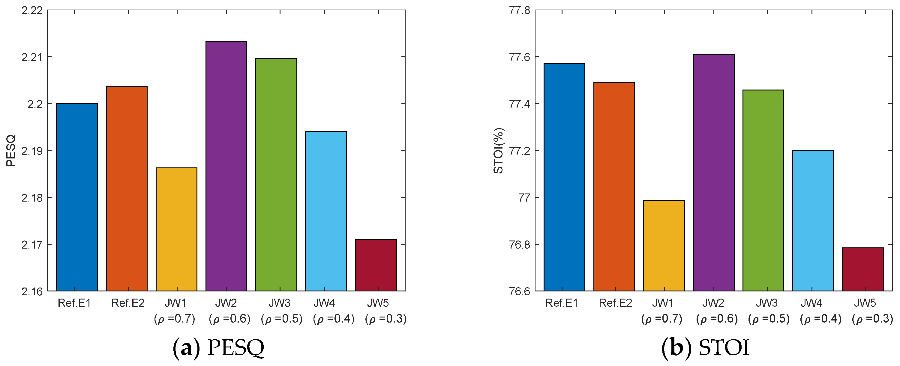
Figure 5 shows the average PESQ and STOI scores for the SMDTANet network trained with all of the aforementioned loss variants on the test dataset. In Figure 5, the weight factors ρ [ 0.7 ,   0.6 ,   0.5 ,   0.4 ,   0.3 ] are examined. All tests use the same post-processing way as in Section 5.1.1. In addition, all tests are based on the same SMDTANet architecture, and other experimental settings are the same.
Compared with several variants with different ρ values in Figure 5, we can find that a choice of ρ value in the JW loss function being very close to 0.6 brings the best perceptual speech quality and the highest speech intelligibility. For instance, the JW2 using ρ = 0.6 improves the average PESQ from 2.171 (JW5), 2.1863 (JW1), 2.194 (JW4), and 2.2097 (JW3) to 2.2133 (JW2). And it also offers the highest STOI score. Furthermore, the setting of ρ = 0.5 , which is close to our chosen one, obtains quite similar PESQ and STOI scores. In comparison, using a very small value of ρ , e.g., ρ = 0.3 , leads to a serious drop in PESQ and STOI values. Accordingly, for this paper, the weighting factor ρ is set to 0.6, which can help to build a more suitable JW loss function for the multi-objective speech enhancement task.
In the macroscopic view, as shown in Figure 5, it becomes obvious that the proposed JW loss function with appropriate setting, i.e., JW2, can offer superior noise attenuation and speech preservation performance compared to other reference functions. Specifically, compared with using Ref. E1 and the Ref. E2, the SMDTANet trained with JW2 can produce substantial performance improvements in terms of PESQ and STOI scores. These findings indicate that our JW loss function can make full use of the advantage of the MA and MSA optimization approach to guide the SMDTANet to obtain more exact mask and spectrogram estimation.

5.2. Comparison with Other Attention Types

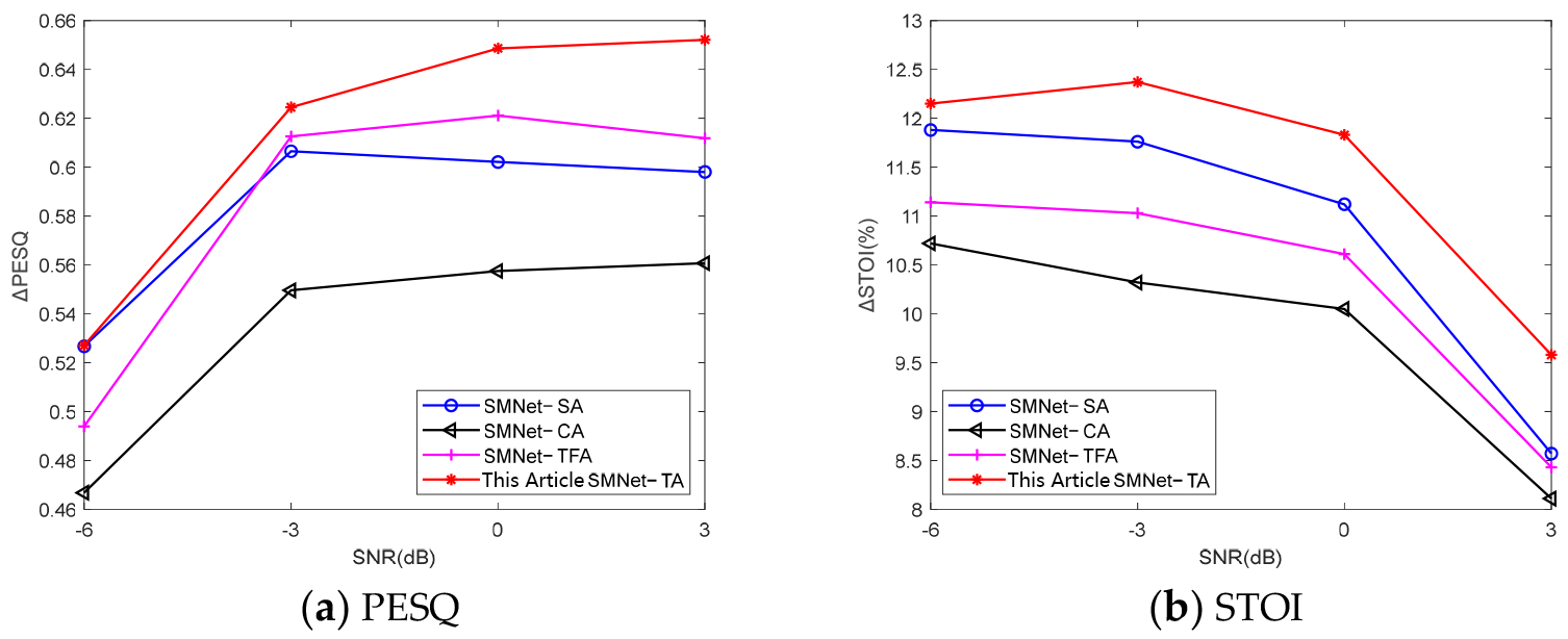
As mentioned in Section 3.2, in the SMDTANet, the proposed TA attention technique is embedded in the TCNN module, which can emphasize the speech-related feature information and boost its temporal modeling capability for speech signals. For simplicity, in this section, we use the SMNet network described in Section 5.1.1 as the backbone structure, which utilizes the original TCNN without any additional attention modules. Then, based on this SMNet architecture, we build and compare several SMNet variants with different types of attention mechanisms to evaluate the effectiveness of the proposed triple-attention module. Specifically, we consider four attention techniques, i.e., channel-wise, spatial, T-F, and the proposed TA attention, to be embedded in the SMNet, respectively, and name their corresponding enhancement networks “SMNet−CA”, “SMNet−SA”, “SMNet−TFA”, and “SMNet−TA” (proposed method), respectively. Figure 6 shows the average PESQ and STOI gains at four SNR levels of the SMNet using different attention modules compared with the scores of mixture speech in the top row of Table 1. All tests adopt the same post-processing way as in Section 5.1.1, and other experimental settings are also the same.
From Figure 6, we observe that our proposed SMNet−TA yields considerable performance improvement in terms of PESQ and STOI at all SNR levels. For example, at 3 dB SNR, by incorporating the TA module into the TCNN, the SMNet−TA improves the average PESQ gain from 0.5607 (SMNet−SA), 0.598 (SMNet−CA), and 0.6118 (SMNet−TFA) to 0.6521 (SMNet−TA) and also increases the average STOI gain from 8.11% (SMNet−SA), 8.43% (SMNet−TFA), and 8.57% (SMNet−CA) to 9.58% (SMNet−TA). Even under an extremely low SNR (−6 dB), the SMNet−TA again outperforms others, giving 0.527 gains in PESQ and 12.15% gains in STOI. These results indicate that our proposed triple attention module made up of channel, spatial, and T-F attention can capture significant information on the input features from different perspectives and gain better signal representation to further improve the network performance in modeling temporal dependencies of speech.

5.3. Overall Performance Comparison

In this section, we compare the proposed method with different types of speech enhancement algorithms to assess its effectiveness. Specifically, seven well-known speech enhancement methods are chosen as reference baselines, namely LSTM, STCNN, CRN, GCRN, FullSubNet, GaGNet, and DeepFilterNet. More details about these methods are provided in Section 4.2. Table 3 shows the average PESQ and STOI scores of the proposed method and the other seven reference methods on the test set at all SNR levels across 11 unseen noise types. In the first column of Table 3, “b1–b4” denote four types of realistic airborne noise, and the other seven labels (namely “car, train, restaurant, airport, exhibition, subway, and street”) obtained from the Aurora noise library are used to represent mismatched society noise. Notably, in Table 3, “SMDTANet” refers to our SMDTANet model trained with the proposed JW loss function as described in Equation (21). In addition, to investigate the overall performance of our method, we use the average post-processing way [11] to reconstruct the enhanced waveform for all multi-objective methods, including LSTM, STCNN, and SMDTANet.
From Table 3, one can observe that our method consistently outperforms all reference methods in two metric scores for most cases. Specifically, we first observe that SMDTANet yields better objective quality and intelligibility scores than LSTM and STCNN, both of which are highly homologous to SMDTANet since they all are based on the multi-objective speech enhancement framework. For example, compared with LSTM and STCNN, SMDTANet improves on average by 10.65% and 6.97% in terms of the PESQ, respectively. And the average STOI gains are 6.48% and 2.8%, respectively. Those improvements indicate that the proposed network topology is more appropriate for the multi-objective enhancement task. Then, to further evaluate the overall performance of our method, we compare SMDTANet with five state-of-the-art methods, i.e., CRN, GCRN, FullSubNet, GaGNet, and DeepFilterNet. Obviously, the five methods underperform the proposed SMDTANet. Specifically, in terms of the PESQ, SMDTANet obtains an average increase of 0.1777, 0.1492, 0.115, 0.057, and 0.02, accounting for 8.72%, 7.23%, 5.48%, and 2.63% improvement over the CRN, GCRN, FullSubNet, and GaGNet, respectively. And SMDTANet also obtains comparable and even better PESQ scores than DeepFilterNet. From an alternative perspective, our SMDTANet also obtains substantial improvements in STOI compared to CRN, GCRN, FullSubNet, GaGNet, and DeepFilterNet.
There are two main reasons for this. One reason is that our SMDTANet architecture has good noise robustness due to the utilization of the stacked multiscale feature extractor, the TA-TCNN, and the densely connected prediction module. Specifically, the stacked multiscale feature extractor can capture implicit acoustic correlations in the broader receptive field, which can filter noise components in the contaminated utterances and rectify coarse vocal characteristics. The TA-TCNN uses multiple attention mechanisms to emphasize feature representation, which can further promote speech quality. The densely connected prediction module can boost feature transmission and alleviate the vanishing gradient issue, which can also help suppress noise and recover high-quality enhanced speech magnitude. Another reason is that SMDTANet optimizes the network by maximizing the JW objective function. The proposed JW loss function that leverages the merit of the mask approximation and signal approximation objective can further refine the learning process of the masking target and consequently improve the noise attenuation and speech recovery ability of the whole system.
Overall, all these findings in Table 3 imply that the proposed SMDTANet model optimized with the proposed JW objective function can significantly filter residual noise interferences and retain the sound integrity to a greater extent, even in the untrained airborne noise scenario.

5.4. Enhanced Spectrogram Comparison

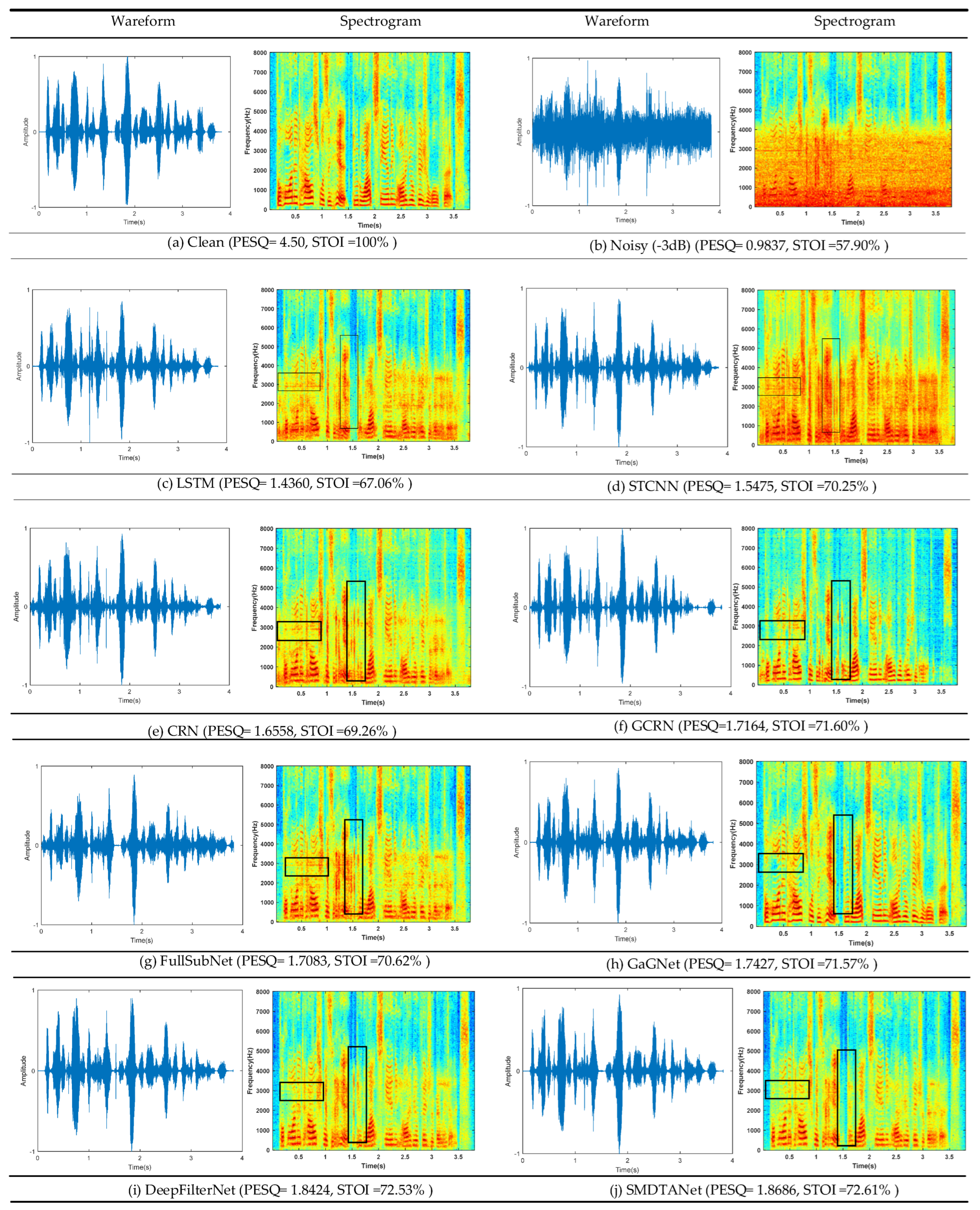
To intuitively and simply present the superiority of the proposed SMDTANet method in speech enhancement, in this section, we examine the enhanced waveforms and spectrograms produced by our method and other reference algorithms. Figure 7 presents the waveform and spectrograms of one representative example with the aircraft tail noise types. We also give the waveforms and spectrograms of the mixture speech signal (at the −3 dB input SNR) and its corresponding clean speech in Figure 7 as a reference.
As shown in Figure 7, one can observe that the enhanced speeches obtained by the LSTM, STCNN, CRN, GCRN, FullSubNet, GaGNet, and DeepFilterNet preserve a large proportion of residual noise interferences, which fully exposes the drawbacks of these methods in purifying invisible noise components and retaining noise robustness in the mismatched noise scenarios. Examples of this phenomenon appear in the 0.20–0.80 s and 1.40–1.60 s sections of Figure 7c–i (in the black solid frames). Furthermore, when compared with the clean spectrogram (Figure 7a), the voice energy of the enhanced speech produced by those seven reference methods is inconspicuous, especially in the range of 2 kHz to 5 kHz. This indicates that those methods will suppress speech segments and cause speech distortions when filtering out airborne noise interference. In comparison, the enhanced spectrogram of our SMDTANet has considerably less residual noise and also has more speech spectral details. From an alternative perspective, we can observe that the waveform enhanced by SMDTANet is well aligned with clean speech. All of these findings demonstrate the effectiveness of our method in noise removal and speech preservation.

6. Conclusions

In this paper, we propose a novel framework, named the stacked multiscale densely connected temporal convolutional attention network (SMDTANet), for multi-objective speech enhancement in real-world airborne noise environments. In the SMDTANet, the proposed stacked multiscale feature extractor is employed to produce contextual information of multiple time scales. Then, the TA-TCNN is designed to emphasize the speech-bearing information from different perspectives, neglect useless noise interference information, and, consequently, improve its temporal modeling power for speech signals. And the densely connected prediction module is introduced to encourage information transmission between each layer for better target estimation. Furthermore, our SMDTANet is optimized using a new joint-weighted loss function to further boost the speech enhancement performance with less extensive computational effort. To demonstrate the effectiveness of our method in both airborne environment and social activity acoustic scenarios, we conducted extensive experiments using the real-world airborne noise data and the widely used ambient noise data acquired from NOISEX92, NONSPEECH, and the Aurora noise library. Meanwhile, we also compared the proposed method with seven advanced deep-learning speech enhancement methods (i.e., LSTM, STCNN, CRN, GCRN, FullSubNet, GaGNet, and DeepFilterNet). The experimental results confirm that the proposed SMDTANet offers much higher noise attenuation as well as better speech listening quality than all reference methods, especially in the realistic airborne scenario.
In the future, we will modify the modeling module to build a magnitude and complex spectral collaborative learning framework. In this way, we expect to incorporate phase information into the proposed approach and further improve speech quality. In addition, we will also extend our method to full-band audio, which is more suitable for a real-world speech enhancement system with high real-time requirements [39].

Author Contributions

Conceptualization, P.H.; Data Curation, Y.W.; Formal Analysis, P.H.; Funding Acquisition, Y.W.; Investigation, P.H.; Methodology, P.H.; Project Administration, Y.W.; Resources, Y.W.; Software, P.H.; Supervision, Y.W.; Validation, P.H.; Visualization, P.H.; Writing—Original Draft, P.H.; Writing—Review and Editing, Y.W. All authors have read and agreed to the published version of the manuscript.

Funding

This research received no external funding.

Institutional Review Board Statement

Not applicable.

Data Availability Statement

Most of the data supporting the conclusions of this paper are available in the Timit corpus [31], NOISEX92 [32], NONSPEECH [33], and AUROR [34] databases.

Conflicts of Interest

The authors declare no conflicts of interest.

Abbreviations

T-FTime–frequency
LPSLog-power spectra
AMSAmplitude modulation spectrogram
IRMIdeal ratio mask
MOLMulti-objective learning
DFTDiscrete Fourier transform
DNNDeep neural network
MLPMulti-layer perception
RNNRecurrent neural network
CNNConvolutional neural network
LSTMLong short-term memory
TCNNTemporal convolutional neural network
STCNNStacked and temporal convolutional neural network
CRNConvolutional recurrent network
GCRNGated convolutional recurrent network
FullSubNetFull-band and sub-band fusion network
GaGNetGlance and gaze network
D-convDepth-wise convolution
SMDTANetStacked multiscale densely connected temporal convolutional attention network
MS-blockMultiscale convolution block
TA-TCNNTriple-attention-based temporal convolutional neural network
CSAChannel–spatial attention
DCDensely connected
ERBEquivalent rectangular bandwidth
ReLURectifying linear unit
BNBatch normalization
MSEMean-square error
MAMask approximation
MSAMask-based signal approximation
JWJoint weighted
MMillion
GFLOPsGiga-floating-point operations per second
SNRSignal-to-noise ratio
PESQPerceptual evaluation of speech quality
STOIShort-time objective intelligibility
RTFReal-time factor

References

  1. Boll, S. Suppression of acoustic noise in speech using spectral subtraction. IEEE Trans. Acoust. Speech Signal Process. 1979, 27, 113–120. [Google Scholar] [CrossRef]
  2. Lim, J.; Oppenheim, A. All-pole modeling of degraded speech. IEEE Trans. Acoust. Speech Signal Process. 1978, 26, 197–210. [Google Scholar] [CrossRef]
  3. Ephraim, Y.; Van Trees, H.L. A signal subspace approach for speech enhancement. IEEE Trans. Speech Audio Process. 1995, 3, 251–266. [Google Scholar] [CrossRef]
  4. Li, A.; Yuan, M.; Zheng, C.; Li, X. Speech enhancement using progressive learning-based convolutional recurrent neural network. Appl. Acoust. 2020, 166, 107347. [Google Scholar] [CrossRef]
  5. Ren, X.; Chen, L.; Zheng, X.; Xu, C.; Zhang, X.; Zhang, C.; Guo, L.; Yu, B. A neural beamforming network for b-format 3d speech enhancement and recognition. In Proceedings of the 2021 IEEE 31st International Workshop on Machine Learning for Signal Processing (MLSP), Gold Coast, Australia, 25–28 October 2021; IEEE: New York, NY, USA, 2021; pp. 1–6. [Google Scholar]
  6. Xiang, X.; Zhang, X. Joint waveform and magnitude processing for monaural speech enhancement. Appl. Acoust. 2022, 200, 109077. [Google Scholar] [CrossRef]
  7. Saleem, N.; Khattak, M.I.; Al-Hasan, M.; Qazi, A.B. On learning spectral masking for single channel speech enhancement using feedforward and recurrent neural networks. IEEE Access 2020, 8, 160581–160595. [Google Scholar] [CrossRef]
  8. Taherian, H.; Wang, Z.Q.; Chang, J.; Wang, D. Robust speaker recognition based on single-channel and multi-channel speech enhancement. IEEE/ACM Trans. Audio Speech Lang. Process. 2020, 28, 1293–1302. [Google Scholar] [CrossRef]
  9. Wang, Y.; Han, J.; Zhang, T.; Qing, D. Speech enhancement from fused features based on deep neural network and gated recurrent unit network. EURASIP J. Adv. Signal Process. 2021, 2021, 104. [Google Scholar] [CrossRef]
  10. Jia, X.; Li, D. TFCN: Temporal-frequential convolutional network for single-channel speech enhancement. arXiv 2022, arXiv:2201.00480. [Google Scholar]
  11. Wang, Q.; Du, J.; Dai, L.R.; Lee, C.H. A Multiobjective Learning and Ensembling Approach to High-Performance Speech Enhancement with Compact Neural Network Architectures. IEEE/ACM Trans. Audio Speech Lang. Process. 2018, 26, 1185–1197. [Google Scholar] [CrossRef]
  12. Zhou, L.; Chen, X.; Wu, C.; Zhong, Q.; Cheng, X.; Tang, Y. Speech Enhancement via Residual Dense Generative Adversarial Network. Comput. Syst. Sci. Eng. 2021, 38, 279–289. [Google Scholar] [CrossRef]
  13. Haridas, A.V.; Marimuthu, R.; Chakraborty, B. A novel approach to improve the speech intelligibility using fractional delta-amplitude modulation spectrogram. Cybern. Syst. 2018, 49, 421–451. [Google Scholar] [CrossRef]
  14. Wang, X.; Bao, F.; Bao, C. IRM estimation based on data field of cochleagram for speech enhancement. Speech Commun. 2018, 97, 19–31. [Google Scholar] [CrossRef]
  15. Xu, Y.; Du, J.; Dai, L.R.; Lee, C.H. A regression approach to speech enhancement based on deep neural networks. IEEE/ACM Trans. Audio Speech Lang. Process. 2014, 23, 7–19. [Google Scholar] [CrossRef]
  16. Fujimura, T.; Koizumi, Y.; Yatabe, K.; Miyazaki, R. Noisy-target training: A training strategy for DNN-based speech enhancement without clean speech. In Proceedings of the 2021 29th European Signal Processing Conference (EUSIPCO), Dublin, Ireland, 23–27 August 2021; IEEE: New York, NY, USA, 2021; pp. 436–440. [Google Scholar]
  17. Chen, J.; Wang, D.L. Long short-term memory for speaker generalization in supervised speech separation. J. Acoust. Soc. Am. 2017, 141, 4705–4714. [Google Scholar] [CrossRef] [PubMed]
  18. Sun, L.; Du, J.; Dai, L.R.; Lee, C.H. Multiple-target deep learning for LSTM-RNN based speech enhancement. In Proceedings of the 2017 Hands-Free Speech Communications and Microphone Arrays (HSCMA), San Francisco, CA, USA, 1–3 March 2017; IEEE: New York, NY, USA, 2017; pp. 136–140. [Google Scholar]
  19. Pandey, A.; Wang, D.L. TCNN: Temporal convolutional neural network for real-time speech enhancement in the time domain. In Proceedings of the ICASSP 2019—2019 IEEE International Conference on Acoustics, Speech and Signal Processing (ICASSP), Brighton, UK, 12–17 May 2019; IEEE: New York, NY, USA, 2019; pp. 6875–6879. [Google Scholar]
  20. Li, R.; Sun, X.; Li, T.; Zhao, F. A multi-objective learning speech enhancement algorithm based on IRM post-processing with joint estimation of SCNN and TCNN. Digit. Signal Process. 2020, 101, 102731. [Google Scholar] [CrossRef]
  21. Weninger, F.; Hershey, J.R.; Le Roux, J.; Schuller, B. Discriminatively trained recurrent neural networks for single-channel speech separation. In Proceedings of the 2014 IEEE Global Conference on Signal and Information Processing (GlobalSIP), Atlanta, GA, USA, 3–5 December 2014; IEEE: New York, NY, USA, 2014; pp. 577–581. [Google Scholar]
  22. Liu, Y.; Zhang, H.; Zhang, X.; Yang, L. Supervised speech enhancement with real spectrum approximation. In Proceedings of the ICASSP 2019—2019 IEEE International Conference on Acoustics, Speech and Signal Processing (ICASSP), Brighton, UK, 12–17 May 2019; IEEE: New York, NY, USA, 2019; pp. 5746–5750. [Google Scholar]
  23. Xu, C.; Rao, W.; Chng, E.S.; Li, H. Spex: Multi-scale time domain speaker extraction network. IEEE/ACM Trans. Audio Speech Lang. Process. 2020, 28, 1370–1384. [Google Scholar] [CrossRef]
  24. Ye, J.X.; Wen, X.C.; Wang, X.Z.; Xu, Y.; Luo, Y.; Wu, C.L.; Chen, L.Y.; Liu, K. HGM-TCNet: Gated Multi-scale Temporal Convolutional Network using Emotion Causality for Speech Emotion Recognition. Speech Commun. 2022, 145, 21–35. [Google Scholar] [CrossRef]
  25. Woo, S.; Park, J.; Lee, J.Y.; Kweon, I.S. Cbam: Convolutional block attention module. In Proceedings of the European Conference on Computer Vision (ECCV), Munich, Germany, 8–14 September 2018; pp. 3–19. [Google Scholar]
  26. Zhang, Q.; Qian, X.; Ni, Z.; Nicolson, A.; Ambikairajah, E.; Li, H. A Time-Frequency Attention Module for Neural Speech Enhancement. IEEE/ACM Trans. Audio Speech Lang. Process. 2022, 31, 462–475. [Google Scholar] [CrossRef]
  27. Jeihouni, P.; Dehzangi, O.; Amireskandari, A.; Dabouei, A.; Rezai, A.; Nasrabadi, N.M. Superresolution and Segmentation of OCT Scans Using Multi-Stage Adversarial Guided Attention Training. In Proceedings of the ICASSP 2022–2022 IEEE International Conference on Acoustics, Speech and Signal Processing (ICASSP), Singapore, 22–27 May 2022; IEEE: New York, NY, USA, 2022; pp. 1106–1110. [Google Scholar]
  28. Hu, J.; Shen, L.; Sun, G. Squeeze-and-excitation networks. In Proceedings of the IEEE Conference on Computer Vision and Pattern Recognition, Salt Lake City, UT, USA, 18–23 June 2018; pp. 7132–7141. [Google Scholar]
  29. Xie, J.; He, N.; Fang, L.; Ghamisi, P. Multiscale densely-connected fusion networks for hyperspectral images classification. IEEE Trans. Circuits Syst. Video Technol. 2020, 31, 246–259. [Google Scholar] [CrossRef]
  30. Zhou, T.; Ye, X.; Lu, H.; Zheng, X.; Qiu, S.; Liu, Y. Dense convolutional network and its application in medical image analysis. BioMed Res. Int. 2022, 2022, 2384830. [Google Scholar] [CrossRef]
  31. Garofolo, J.S.; Lamel, L.F.; Fisher, W.M.; Fiscus, J.G.; Pallett, D.S.; Dahlgren, N.L. DARPA TIMIT Acoustic-Phonetic Continuous Speech Corpus CD-ROM; National Institute of Standards and Technology: Gaithersburg, MD, USA, 1993. [Google Scholar]
  32. Varga, A.; Steeneken, H.J. Assessment for automatic speech recognition: II. NOISEX-92: A database and an experiment to study the effect of additive noise on speech recognition systems. Speech Commun. 1993, 12, 247–251. [Google Scholar] [CrossRef]
  33. Hu, G. 100 Nonspeech Environmental Sounds. 2004. Available online: http://www.cse.ohio.state.edu/pnl/corpus/HuCorpus.html (accessed on 1 May 2021).
  34. Hirsch, H.G.; Pearce, D. The AURORA experimental framework for the performance evaluations of speech recognition systems under noisy conditions. In Proceedings of the ASR2000-Automatic Speech Recognition: Challenges for the New Millenium International, Speech Communication Association (ISCA) Tutorial and Research Workshop (ITRW), Paris, France, 18–20 September 2000; pp. 181–188. [Google Scholar]
  35. Tan, K.; Wang, D.L. A convolutional recurrent neural network for real-time speech enhancement. Interspeech 2018, 2018, 3229–3233. [Google Scholar]
  36. Tan, K.; Wang, D.L. Learning complex spectral mapping with gated convolutional recurrent networks for monaural speech enhancement. IEEE/ACM Trans. Audio Speech Lang. Process. 2019, 28, 380–390. [Google Scholar] [CrossRef]
  37. Hao, X.; Su, X.; Horaud, R.; Li, X. Fullsubnet: A full-band and sub-band fusion model for real-time single-channel speech enhancement. In Proceedings of the ICASSP 2021—2021 IEEE International Conference on Acoustics, Speech and Signal Processing (ICASSP), Toronto, ON, Canada, 6–11 June 2021; IEEE: New York, NY, USA, 2021; pp. 6633–6637. [Google Scholar]
  38. Li, A.; Zheng, C.; Zhang, L.; Li, X. Glance and gaze: A collaborative learning framework for single-channel speech enhancement. Appl. Acoust. 2022, 187, 108499. [Google Scholar] [CrossRef]
  39. Schröter, H.; Rosenkranz, T.; Maier, A. DeepFilterNet: Perceptually Motivated Real-Time Speech Enhancement. arXiv 2023, arXiv:2305.08227. [Google Scholar]
  40. Kingma, D.P.; Ba, J. Adam: A method for stochastic optimization. arXiv 2014, arXiv:1412.6980. [Google Scholar]
  41. ARix, W.; Beerends, J.G.; Hollier, M.P.; Hekstra, A.P. Perceptual evaluation of speech quality (PESQ)—A new method for speech quality assessment of telephone networks and codecs. In Proceedings of the 2001 IEEE International Conference on Acoustics, Speech, and Signal Processing, Salt Lake City, UT, USA, 7–11 May 2001; pp. 749–752. [Google Scholar]
  42. Taal, C.H.; Hendriks, R.C.; Heusdens, R.; Jensen, J. An algorithm for intelligibility prediction of time–frequency weighted noisy speech. IEEE Trans. Audio Speech Lang. Process. 2011, 19, 2125–2136. [Google Scholar] [CrossRef]
  43. Lu, Z.; Rallapalli, S.; Chan, K.; La Porta, T. Modeling the resource requirements of convolutional neural networks on mobile devices. In Proceedings of the 25th ACM international conference on Multimedia, Mountain View, CA, USA, 23–27 October 2017; pp. 1663–1671. [Google Scholar]
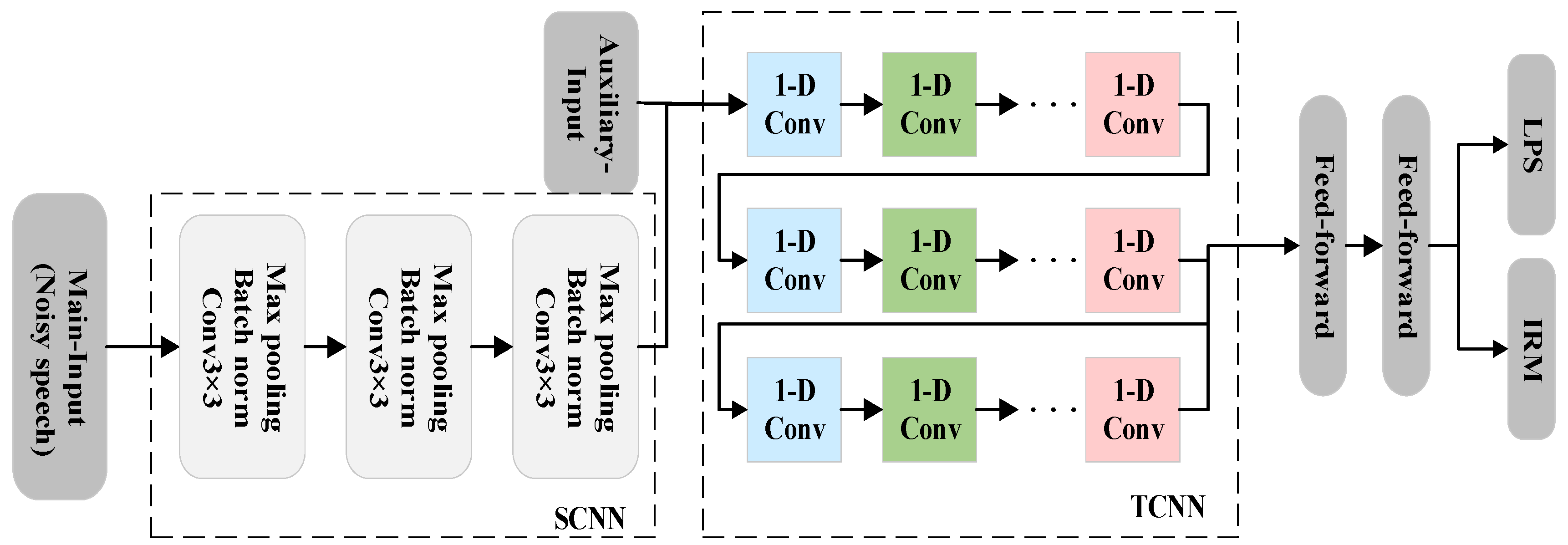
Figure 1. Illustration of the STCNN for multi-objective speech enhancement in [20]. The STCNN comprises three modules: a stacked convolutional neural network (SCNN), a temporal convolutional neural network (TCNN), and two feed-forward layers.
Aerospace 11 00156 g001
Figure 2. The detailed architecture of TCNN.
Aerospace 11 00156 g002
Figure 3. Block diagram of the proposed SMDTANet. (a) The overview diagram of the SMDTANet, which comprises three modules: a stacked multiscale feature extractor, a TA-TCNN, and a densely connected prediction module. (b) The detailed structure of a multiscale convolution block (MS-block). (c) The detailed structure of a densely connected (DC) block. “TA” denotes the triple-attention module.
Aerospace 11 00156 g003
Figure 4. A diagram of the proposed triple-attention module, which comprises a channel–spatial attention block and a T-F attention block. Here, and denote the element-wise product and matrix multiplication, respectively.
Aerospace 11 00156 g004
Figure 5. The average PESQ and STOI performance for the SMDTANet using different loss functions on the unseen test set across all SNR levels.
Aerospace 11 00156 g005
Figure 6. Average gains in terms of PESQ and STOI for the baseline SMNet using different attention types compared with the PESQ and STOI scores of noisy speech.
Aerospace 11 00156 g006
Figure 7. Comparison of enhanced waveforms and spectrograms using different methods in the aircraft tail noise case at the −3 dB SNR level.
Aerospace 11 00156 g007
Table 1. Composition of the airborne noises used in our work.
DatasetNoise Source Noise TypeTotal Number
Training setReal-time acquisition in the cockpit of aircraft AEngine fire alarms, aircraft taxiing noise, aircraft take-off noise, aircraft landing noise, aircraft fault noise, and stall alarm noise.8
Test setReal-time acquisition in the cockpit of aircraft BAircraft tail noise, high-frequency metal scratching noise, propeller noise, and space noise in the aircraft cabin.4
Table 2. The performance in terms of PESQ, STOI (%), model size (in millions), and GFLOPs in the ablation study under the unseen noise scenario. The BOLD values indicate the best performance. “-” denotes that the result is not provided in the original paper.
MethodModel Size (M)GFLOPsRTFPESQ (Score)STOI (%)
SNR Level (dB)AvgSNR Level (dB)Avg
30−3−630−3−6
Noisy---1.8581.63981.42261.25561.54475.4769.0762.5255.2165.57
STCNN---2.41872.19171.95071.71452.0689 84.8179.4272.7365.0175.49
SMNet 7.468.040.03692.47272.22781.98521.75992.1184.8579.9173.3965.8976.01
SMNet-TA+0.8+0.710.05672.51012.28842.04711.78262.15785.0580.974.8967.3677.05
SMDTANet+3.84+3.310.0862.5512.33042.09771.83372.2085.4681.275.2468.3777.57
Table 3. The average performance comparisons of our method and different reference methods on the test set across 11 unseen noise types at all SNR levels. The best performers are highlighted in BOLD font.
Noise TypePESQ (Score)
LSTMSTCNNCRNGCRNFullSubNetGaGNetDeepFilterNetSMDTANet
b12.6327 2.6800 2.7158 2.6957 2.7596 2.7366 2.80112.8232
restaurant1.8861 1.9614 1.9468 1.9956 2.0118 2.0033 2.06192.0948
car1.9855 2.1000 2.0332 1.9989 2.1786 2.2238 2.26532.2990
b22.1092 2.3296 2.1025 2.1502 2.2620 2.3656 2.4662.4896
b31.8697 1.9620 1.9500 1.9486 2.1052 2.1079 2.15012.1376
airport2.1052 2.1591 2.1444 2.0920 2.2027 2.2099 2.24542.2753
train2.5627 2.5698 2.5762 2.6380 2.6772 2.6507 2.72042.7518
exhibition1.5373 1.6571 1.6237 1.7853 1.8066 1.8728 1.90551.9227
b41.7467 1.5409 1.5804 1.4919 1.2047 1.4901 1.33061.3355
subway2.1975 2.2799 2.2727 2.2616 2.3114 2.3089 2.38222.4050
street1.3713 1.5184 1.4464 1.6472 1.5602 1.7531 1.79051.8120
Average2.0003 2.0689 2.0356 2.0641 2.0982 2.1566 2.19262.2133
Noise TypeSTOI (%)
LSTMSTCNNCRNGCRNFullSubNetGaGNetDeepFilterNetSMDTANet
b184.50 86.48 85.74 85.19 86.24 86.39 87.5687.34
restaurant 69.90 72.57 72.02 75.68 72.00 72.37 74.0274.58
car72.87 76.15 74.78 74.21 76.45 77.40 78.8879.18
b279.08 83.53 80.22 82.82 81.63 82.91 84.2184.64
b365.66 69.44 68.21 70.45 73.05 72.61 73.2272.95
airport75.66 77.97 77.34 82.52 76.76 77.37 78.7479.38
train86.17 87.32 86.05 86.45 86.68 86.67 87.1387.97
exhibition65.59 68.00 66.80 70.63 72.01 72.28 72.6672.78
b464.21 65.21 63.23 69.29 60.87 66.03 65.0164.75
subway78.42 80.70 79.40 78.35 79.64 79.63 81.7181.30
street59.71 63.02 60.85 63.45 63.62 67.75 68.668.86
Average72.89 75.49 74.06 76.28 75.36 76.49 77.4377.61
Disclaimer/Publisher’s Note: The statements, opinions and data contained in all publications are solely those of the individual author(s) and contributor(s) and not of MDPI and/or the editor(s). MDPI and/or the editor(s) disclaim responsibility for any injury to people or property resulting from any ideas, methods, instructions or products referred to in the content.