Data-Driven Sensitivity Analysis of the Influence of Geometric Parameterized Variables on Flow Fields Under Different Design Spaces

Abstract

In aerodynamic shape optimization, geometric parameterized variables have a significant impact on the flow field, thereby influencing both the effectiveness and efficiency of the optimization process. This paper utilizes flow field data from computational fluid dynamics (CFD) to develop a data-driven approach for analyzing the influence of geometric parameterized variables on the objective function and flow field across various design spaces. A data-driven method, namely a sensitivity analysis based on the Kriging model, is proposed along with three design space variation schemes (scaling, translation, and their combination) to evaluate the influence of geometric parameters on the objective function under varying design spaces. Furthermore, the study investigates the effects of these design space variation schemes on the sensitivity results using two test functions and a wave drag reduction case. The results of the wave drag reduction case are further analyzed in relation to flow conditions, including the Mach number and shock-wave strength. The findings indicate that design space variations alter the relationship between geometric parameters and the flow field, particularly affecting the shock-wave position and strength, as reflected by the sensitivity indices of the variables. Additionally, the sensitivity results show a strong dependence on the Mach number under varying design space configurations.

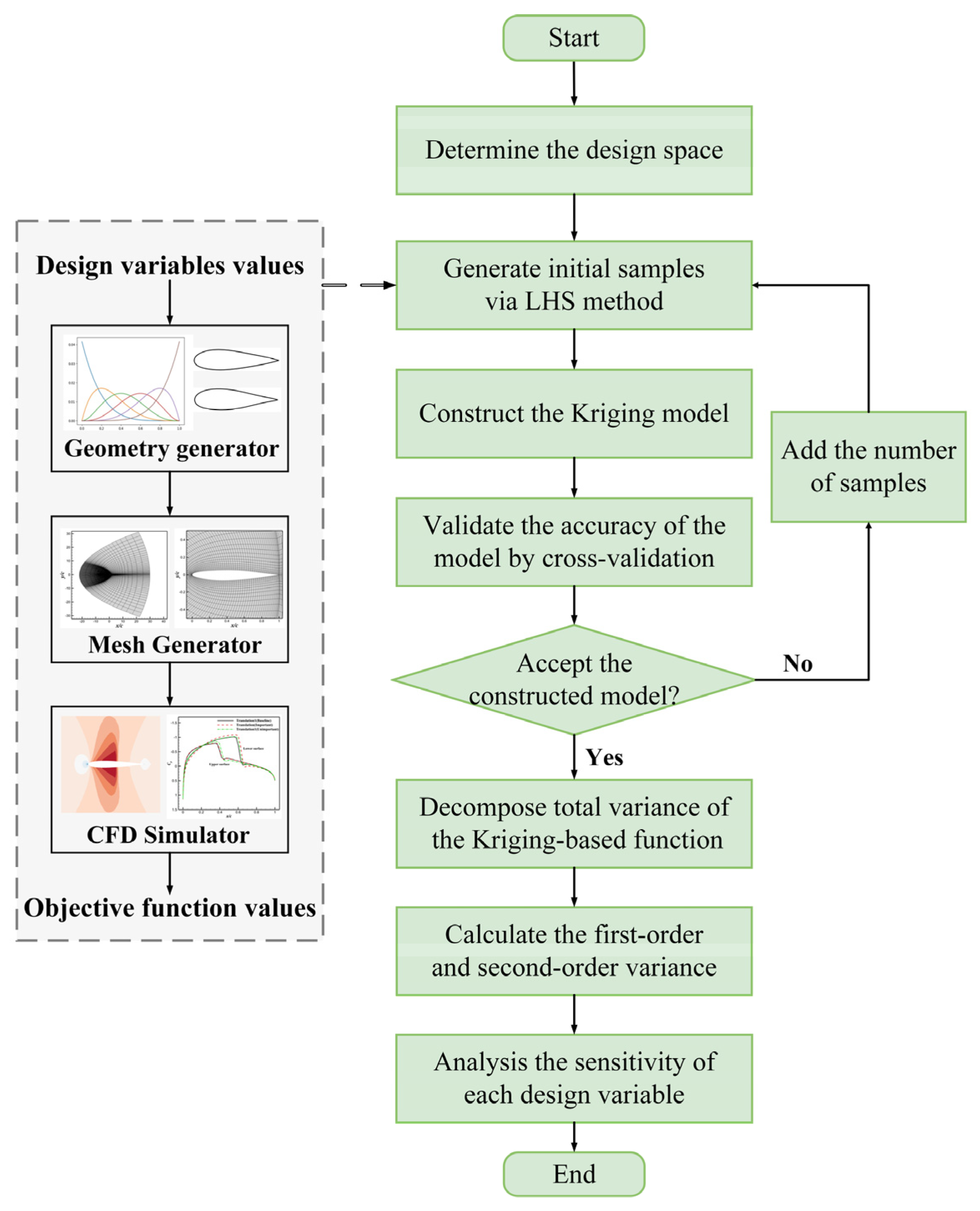
1. Introduction

The aerodynamic shape of an aircraft significantly influences its performance, making aerodynamic shape design a critical component in aircraft development. With advancements in computational capabilities, aerodynamic shape optimization (ASO), which integrates computational fluid dynamics (CFD) technology with optimization algorithms, has become a fundamental method in contemporary aircraft design [1,2,3,4]. To establish an accurate physical model for flow field solutions, a comprehensive set of design variables is typically employed during the geometric shape parameterization stage to fully capture the geometric characteristics of the shape [5]. However, this approach often results in a substantial increase in both the number of design variables and the associated computational costs. As the number of design variables increases, the dimensionality of the design space expands, complicating the optimization problem and reducing optimization efficiency [6,7,8]. Therefore, achieving a balance between optimization effectiveness and computational cost reduction remains a major challenge in ASO.

To balance optimization efficiency and effectiveness in ASO, researchers have investigated several approaches, including surrogate modeling, dimensionality reduction, and variable screening techniques [9,10,11,12]. Surrogate models, such as polynomial response surfaces [13], Kriging [14], radial basis functions [15], and neural networks [16,17], are often used to approximate complex CFD simulations, thereby reducing computational costs and enhancing optimization efficiency. However, due to their strong reliance on training data, these methods often encounter issues such as limited accuracy and poor generalizability, which pose significant challenges, especially in high-dimensional problems. In addition, dimensionality reduction techniques, such as Proper Orthogonal Decomposition (POD), Principal Component Analysis (PCA), and Self-Organizing Map(SOM, have been employed to project high-dimensional design spaces into lower-dimensional representations while preserving key features of the original design. This reduces the number of variables involved and improves computational efficiency [18,19,20]. However, while dimensionality reduction can simplify the design space, it may also result in a loss of parameterization accuracy, which could hinder the achievement of truly optimal solutions. Thus, balancing the trade-off between reduced optimization effectiveness and increased efficiency remains a considerable challenge in the application of dimensionality reduction techniques.

Variable screening methods, particularly sensitivity analysis, represent another key approach to improving optimization efficiency and have been widely applied across various engineering disciplines [21,22,23,24]. Sensitivity analysis, also known as variable importance analysis, identifies input parameters that have a significant impact on outputs while disregarding less influential variables [25]. This process reduces the dimensionality of the design space, decreases problem complexity, and enhances optimization efficiency. Furthermore, by pinpointing and prioritizing key design variables, sensitivity analysis provides essential insights into the interactions between inputs and outputs, which are essential for guiding design decisions and improving the interpretability of complex models. There are many sensitivity analysis methods, including the Morris method, Sobol’s method, and the functional variance analysis method, among others. These methods have been widely applied in various fields to address optimization problems. For instance, Lai et al. [26] applied Sobol’s sensitivity analysis to investigate lithium-ion batteries used in electric vehicles. Jeong et al. [27] proposed an efficient optimization method for aircraft design that analyzed variable sensitivity through functional analysis of variance. Xu et al. [28] introduced an optimization method based on design variable screening. Utilizing a data-driven method that integrates the Kriging regression model with functional analysis of variance, their approach quantitatively assesses the influence of design variables on the objective function and incorporates a screening strategy to reduce both problem dimensionality and computational costs. However, each method has its own strengths and limitations. The Morris method is computationally efficient but cannot capture higher-order effects, while Sobol’s method provides comprehensive sensitivity indices, including first-order and interaction effects. Nevertheless, it relies on multi-dimensional integration and requires a large number of samples to compute sensitivity indices, resulting in high computational costs. To address these challenges, this paper adopts the functional variance analysis method, which improves efficiency by utilizing a Kriging model to transform high-dimensional integrals into one-dimensional integrals.

In the aforementioned variance-based sensitivity analysis method, calculating the response variance of each variable requires traversing the entire design space [29,30]. As a result, selecting an appropriate design space is critical for ensuring the accuracy of sensitivity analysis results and demands careful consideration of the design range for each variable. In ASO, the ranges of design variables are typically determined subjectively by designers based on engineering experience, which introduces uncertainty into the definition of these variable ranges [31]. During the optimization process, the parameterization phase often involves incorporating as many design variables as possible to capture geometric uncertainty and explore a broader range of potential shapes. However, many of these variables may not directly influence the objective function but instead induce only minor modifications to the geometric shape. Consequently, adjusting the range of these design variables may be redundant In the optimization process.

In practical engineering applications, when the relationship between design variables and the objective function is uncertain, timely adjustments to the variable ranges during the optimization process are crucial for identifying the optimal search region. However, flow problems often exhibit complex characteristics such as multi-peaked behavior and nonlinearity [32,33], and the shape and trend of the objective function vary across different design ranges, leading to substantial variations in the flow field. Consequently, in various optimization contexts, even when targeting the same objective function, the optimization goals may differ due to these variations. Based on the preceding discussion and analysis, it is evident that existing research lacks a clear definition or distinction regarding the scope of design variables. Therefore, this study aims to investigate the impact of variations in the scope of design variables on the outcomes of variance-based global sensitivity analysis methods. Moreover, the study explores the influence of selected design variables on the flow field, providing theoretical guidance for aerodynamic shape optimization.

The structure of this paper is organized as follows: Section 2 provides a detailed introduction to the data-driven method employed in this study. Section 3 introduces and discusses three design space variation schemes: scaling, translation, and combination. Section 4 verifies the feasibility and rationale of these variation schemes by two test functions, followed by a comprehensive analysis of these results. Section 5 applies the proposed design space variation schemes to the wave drag reduction case of the NACA0012 airfoil, along with a detailed analysis of the outcomes. Finally, Section 6 presents the conclusions of this paper.

2. Data-Driven Method: Functional Variance Analysis Method Based on the Kriging Model

The functional variance analysis method based on the Kriging model is a data-driven method that utilizes surrogate modeling techniques to quantify and analyze the variance in functional responses caused by multiple design variables. This section introduces the functional variance analysis method based on the Kriging model. The functional variance analysis method is a global sensitivity analysis technique that quantifies the contribution of each design variable to the objective function by decomposing the total variance of the function. To implement this method, it is necessary to establish a relationship between the design variables and the objective function. In this study, the Kriging model is used to construct an approximate expression for this relationship. Figure 1 shows the flowchart of the functional variance analysis method based on the Kriging model.

This section includes details on the Kriging model and functional variance decomposition. Additionally, a two-dimensional test function is used to validate the accuracy and effectiveness of this method.

2.1. Kriging Model

The Kriging model is used to construct an approximate model function for variance analysis based on the distribution information of design variables. It can give the best linear prediction value and mean square error of unknown points by existing samples. The mathematical expression of the Kriging model is as follows:

$$f(x)=\phi {(x)}^{\mathrm{T}}\cdot \eta +z(x)$$

(1)

where $\phi (x)$ is a polynomial of $x$, $\eta$ is the regression coefficient, and $\phi (x)\cdot \eta$ represents the global trend function. Generally, $\phi (x)\cdot \eta$ is assumed as the form of a constant, linear, or quadratic term, though the choice of form has minimal impact on prediction results. In this paper, $\phi (x)\cdot \eta$ is taken as a constant value $\mu$. $z(x)$ is a realization of a normally distributed Gaussian random process with a zero mean and ${\sigma }^2$ variance, which presents the deviation from the global trend function. Its covariance can be expressed as follows:

$$\mathrm{cov}(z(x^i),z(x^j))={\sigma }^{2}R(x^i,x^j,\theta )$$

(2)

where $R(x^i,x^j,\theta )$ denotes the spatial correlation function between two random sample points $x^i$ and $x^j(i,j=1,2,3\cdots ,s)$. $\theta$ is the correlation parameter vector, $0<\theta <1$. In this paper, the Gaussian basic function is employed as the correlation function, expressed as follows:

$$R(x^i,x^j,\theta )=e^{-{\displaystyle \sum _{k=1}^n-{\theta }_k{(x_k^i-x_k^j)}^2}}$$

(3)

Given a sample set $x^s={[x^1,x^2,x^3,\cdots ,x^s]}^{\mathrm{T}}$ and their corresponding response values $Y={[g(x^1),g(x^2),g(x^3)\cdots g(x^s)]}^{\mathrm{T}}$, the values of $\mu$ and ${\sigma }^2$ can be estimated by following equation:

$$\begin{array}{l}\mu =(1^{\mathrm{T}}\cdot R^{-1}\cdot Y)/(1^{\mathrm{T}}\cdot R^{-1}\cdot 1)\\ {\sigma }^2=[(Y-\mu \cdot 1)R^{-1}(Y-\mu \cdot 1)]/n\end{array}$$

(4)

where $R={[R_{ij}]}_{s\times s}$, 1 is a $n$-dimensional unit column vector. From the above equation, it can be seen that the equation contains an unknown distribution parameter ${\theta }_k(k=1,2,3\cdots n)$. The value of the unknown distribution parameter is obtained by maximizing the ln-likelihood function using Bayesian optimization algorithm.

Therefore, for a new point $x^{*}\in R^s$, the predicted value of the Kriging model is

$$\widehat{f}(x^{*})=\mu +r^{\mathrm{T}}(x)R^{-1}(Y-\mu \cdot 1)$$

(5)

where $r(x)$ is a n-dimensional correlation coefficient vector, and $r(x)={[R(x^i,x^{*},\theta )]}_{n\times 1}$.

The accuracy of the surrogate model has a direct impact on the result of sensitivity analysis for the design variables. Therefore, it is crucial to verify the accuracy of the constructed Kriging model before conducting sensitivity analysis. If the established model meets the requirement of accuracy, the functional variance analysis can proceed. Otherwise, additional initial samples are added until the accuracy requirement is satisfied. In this study, initial samples are generated using the Latin Hypercube Sampling (LHS) method, and the accuracy of the constructed model is validated through cross-validation. The error of the model is measured by the coefficient of determination $R^2$.

$$R^2=1-{\displaystyle \frac{{\displaystyle {\sum }_{i=1}^s{({\widehat{f}}_{predict}^i-f_{true}^i)}^2}}{{\displaystyle {\sum }_{i=1}^s{(f_{true}^i-\overline{f})}^2}}}$$

(6)

where ${\widehat{f}}_{predict}^i$ represents the predicted value of the Kriging model at the i-th sample, $f_{true}^i$ represents the true value of the function at the i-th sample, $\overline{f}$ represents the mean of all true values across the sample points.

2.2. Functional Variance Decomposition

The core concept of the functional variance analysis method is variance decomposition. Functional variance decomposition involves decomposing the total variance of the function into the sum of the partial variance contributed by individual design variables and their interactions with other design variables. This decomposition provides a quantitative measure of each design variable’s contribution to the objective function. Assuming the input–output relationship of the system can be described by the equation $Y=g(x)$, where $x={[x_1,x_2,x_3,\cdots ,x_n]}^{\mathrm{T}}$ denotes a n-dimensional vector of independent input variables and $Y$ denotes a one-dimensional vector of the output response. The probability density function of each random variable $x_i(i=1,2,3\cdots n)$ is $f_{X_i}(x_i)$, the joint probability density function of $Y$ is $f_X(x)$. When the input variables are independent, the joint probability density function can be expressed as $f_X(x)={\displaystyle \prod _{i=1}^n{f}_{X_i}(x_i)}$. According to the low-dimensional representation of the high-dimensional model, $Y=g(x)$ can be expanded as follows:

$$g(x)=g_0+{\displaystyle \sum _{i=1}^n{g}_i(x_i)}+{\displaystyle \sum _{i_1=1}^n{\displaystyle \sum _{i_2=i_1+1}^n{g}_{i_1,i_2}(x_{i_1,i_2})}}+\cdots g_{1,2,3\cdots n}(x_1,x_2,\cdots ,x_n)$$

(7)

where

$$g_0={\displaystyle \int \dots }{\displaystyle \int g(x){\displaystyle \prod _{i=1}^n[f_{x_i}(x_i)d{x}_i]}}$$

(8)

$$g_i(x_i)={\displaystyle \int \dots }{\displaystyle \int g(x){\displaystyle \prod _{k\ne i}^n[f_{x_k}(x_k)d{x}_k]}}-g_0$$

(9)

$$g_{i_1,i_2}(x_{i_1},x_{i_2})={\displaystyle \int \dots }{\displaystyle \int g(x){\displaystyle \prod _{k\ne i_1,i_2}^n[f_{x_k}(x_k)d{x}_k]}}-g_{i_1}(x_{i_1})-g_{i_2}(x_{i_2})-g_0$$

(10)

where $g_0$ is a constant, the total mean of the function, $g_i(x_i)$ is considered the main effect function, where the design variable $x_i$ is considered individually, $g_{i_1,i_2}(x_{i_1},x_{i_2})$ is the interaction effect function, considering the interactions between two variables $x_i$ and $x_j$.

Calculating the variance by integration on both sides of Equation (7) can obtain

$$V(x)=V_0+{\displaystyle \sum _{i=1}^n{V}_i(x_i)}+{\displaystyle \sum _{i_1=1}^n{\displaystyle \sum _{i_2=i_1+1}^n{V}_{i_1,i_2}(x_{i_1,i_2})}}+\cdots V_{1,2,3\cdots n}(x_1,x_2,\cdots ,x_n)$$

(11)

where $V_i$ is the first-order variance, which denotes the partial variance by a single design variable $x_i$, $V_{i_1,i_2}$ is the second-order variance, which denotes the partial variance by the interaction between two design variables $x_{i_1},x_{i_2}$, and $V_{1,2,3\cdots n}(x_1,x_2,\cdots ,x_n)$ represent higher-order variance.

Based on the previously established Kriging model, the detailed variance expression of the Kriging-based function can be described as follows:

$$g_0={\displaystyle \int \dots {\displaystyle \int [\mu +r^{\mathrm{T}}(x)R^{-1}(Y-\mu \cdot 1)]}}{\displaystyle \prod _{i=1}^{n}d{x}_i}=\mu +{\displaystyle \int \dots {\displaystyle \int [r^{\mathrm{T}}(x)R^{-1}(Y-\mu \cdot 1)]}}{\displaystyle \prod _{i=1}^{n}d{x}_i}$$

(12)

$$V_0={\displaystyle \int \dots {\displaystyle \int [\mu +r^{\mathrm{T}}(x)R^{-1}(Y-\mu \cdot 1)-g_0}}{]}^2{\displaystyle \prod _{i=1}^{n}d{x}_i}$$

(13)

$$g_i={\displaystyle \int \dots {\displaystyle \int [\mu +r^{\mathrm{T}}(x)R^{-1}(Y-\mu \cdot 1)]}}{\displaystyle \prod _{k\ne i}^{n}d{x}_k}=\mu +{\displaystyle \int \dots {\displaystyle \int [r^{\mathrm{T}}(x)R^{-1}(Y-\mu \cdot 1)]}}{\displaystyle \prod _{i\ne i}^{n}d{x}_k}$$

(14)

$$V_i={\displaystyle \int \dots {\displaystyle \int [g_i-g_0}}{]}^2{\displaystyle \prod _{k\ne i}^{n}d{x}_k}$$

(15)

$$g_{i_1,i_2}={\displaystyle \int \dots {\displaystyle \int [\mu +r^{\mathrm{T}}(x)R^{-1}(Y-\mu \cdot 1)]}}{\displaystyle \prod _{k\ne i_1,i_2}^{n}d{x}_k}=\mu +{\displaystyle \int \dots {\displaystyle \int [r^{\mathrm{T}}(x)R^{-1}(Y-\mu \cdot 1)]}}{\displaystyle \prod _{k\ne i_1,i_2}^{n}d{x}_k}$$

(16)

$$V_{i_1,i_2}={\displaystyle \int \dots {\displaystyle \int [g_{i_1,i_2}-g_0}}{]}^2{\displaystyle \prod _{k\ne i_1,i_2}^{n}d{x}_k}$$

(17)

Since high-order variance effects have a negligible impact on the objective function, only the first-order and second-order variances are considered in this paper. The global sensitivity indices derived from functional variance analysis are defined as follows:

$$S_i={\displaystyle \frac{V_i}{V_0}}$$

(18)

$$S_{i,j}={\displaystyle \frac{V_{i,j}}{V_0}}$$

(19)

$$S_i^T=S_i+S_{i,j}$$

(20)

where $S_i$ is the first-order sensitivity index, which quantifies the individual contribution of the design variable $x_i$ to the output and is also referred to as the main effect index. A larger value of $S_i$ indicates a greater contribution of $x_i$ to the output. $S_{i,j}$ represents the second-order sensitivity index, which reflects the contribution of the interaction between design variables $x_i$ and $x_j$ to the output, also known as the interaction effect indices. $S_i^T$ is the overall sensitivity index, representing the total contribution of the design variable $x_i$ to the output and is referred to as the total effect index. A smaller value of $S_i^T$ suggests a lesser contribution of $x_i$ to the output.

2.3. Verification of the Method

Here, a quadratic polynomial function is used to validate the applicability and accuracy of the functional variance analysis method based on the Kriging model. The expression for the quadratic polynomial is given as follows:

$$y(x_1,x_2)=3{x_1}^2+x_2$$

(21)

where $x_1,x_2\in [0,1]$.

Table 1. Analytical results and proposed method of the various variance contributions.

	g0	V0	V1	V2
Analytical results	1.50	0.8833	0.8	0.0833
Sobol’s method	1.5021	0.8899	0.8102	0.0797
Relative error	0.140%	0.7472%	1.275%	4.322%
Proposed method	1.5018	0.8875	0.8053	0.0822
Relative error	0.120%	0.472%	0.662%	1.360%

presents the comparative results of variance obtained from the analytical results, Sobol’s method, and the proposed method. The results show that both Sobol’s method and the proposed method yield variances that are generally consistent with the analytical results. However, the proposed method demonstrates better accuracy, with a relative error of less than 2%. The computational complexity and computational time for the two methods are listed in

Table 2. Comparison of computational complexity and time for sensitivity methods.

Aspect	Computational Complexity	Computational Times (s)
Sobol’s method	O(n*m)	50
Proposed method	O(n)	2

. The computational complexity is measured by Big O notation. It is observed that Sobol’s method has a complexity of O(n*m), while the proposed method achieves a lower complexity of O(n), where n represents the number of design variables, m denotes the number of samples. In terms of computational times, Sobol’s method requires 50 s to complete the sensitivity calculation due to its higher computational complexity. In contrast, the proposed method, benefiting from its reduced complexity, completes the same task in just 2 s. Therefore, it can be concluded that the functional variance analysis method based on the Kriging model is both highly efficient and accurate in obtaining results.

3. Definition and Variation of Design Space

3.1. Definition of Design Space

This paper primarily explores the impact of different design spaces on the results of variance-based sensitivity analysis. Consequently, the method for generating different design spaces becomes a key focus of this research.

In aerodynamic optimization problems, assuming the input variable $x\in R^n$, where each dimensional design variable $x^i(i=1,2,\cdots ,n)$ has its own specified bounds. The design space of the optimization problem can then be represented by two vectors:

$$x_{lower}\le x\le x_{upper}$$

(22)

where vector $x_{lower}$ represents the lower bound and vector $x_{upper}$ represents the upper bounds of the design variable vector.

To provide a more intuitive description of the design space, the center position and size are used to represent the vectors mentioned above. The center position of the design space $c$ is defined as the central value vector of the design variables, expressed as

$$c={[c_1,c_2,c_3,\cdots ,c_n]}^{\mathrm{T}}$$

(23)

where $c_i$ is the center value of the interval for the i-th design variable. The size of the design space, denoted as $r$, is defined as the variation vector of the design variables, expressed as

$$r={[r_1,r_2,r_3,\cdots ,r_n]}^{\mathrm{T}}$$

(24)

where $r_i$ is half the size of the interval for the i-th design variable. The vectors $x_{lower}$ and $x_{upper}$ can be expressed in terms of the center position and the size of the design space as follows:

$$x_{upper}=c-r$$

(25)

$$x_{upper}=c+r$$

(26)

By substituting Equations (25) and (26) into Equation (22), the design space of the optimization problem can be defined as follows:

$$\mathbf{c}-\mathbf{r}\le x\le \mathbf{c}+\mathbf{r}$$

(27)

3.2. Variation of Design Space

Thus, variations in design space can be achieved by altering the center position $c$ and the size $r$. Changing $r$ alone results in the scaling of the design space, while changing $c$ alone results in the translation of the design space. Both $r$ and $c$ can be modified simultaneously to achieve both scaling and translation of the design space.

Scaling of the design space is accomplished through geometric scaling according to a scaling ratio, defined as a vector $\beta ={[{\beta }_1,{\beta }_2,{\beta }_3,\cdots ,{\beta }_n]}^{\mathrm{T}}$, where ${\beta }_i$ represents the scaling factor for the i-th dimensional design variable, ${\beta }_i>0$. The size of the new design space $r^{new}$ can be expressed as follows:

$$r^{new}=\beta \cdot r$$

(28)

By substituting Equation (28) into Equation (27), the scaled design space can be defined as follows:

$$\mathbf{c}-\beta \mathbf{\cdot }r\le x\le \mathbf{c}+\mathbf{\beta }\cdot r$$

(29)

Translation of the design space is achieved by shifting the center position by a specified amount, defined as a translational movement vector $\mathrm{\Delta }c={[\mathrm{\Delta }{c}_1,\mathrm{\Delta }{c}_2,\mathrm{\Delta }{c}_3,\cdots ,\mathrm{\Delta }{c}_n]}^{\mathrm{T}}$, where $\mathrm{\Delta }{c}_i$ represents the movement of the i-th dimensional design variable, $\mathrm{\Delta }{c}_i\in \mathrm{R}$. The center position of the new design space $c^{new}$ can be expressed as follows:

$$c^{new}=c+\mathrm{\Delta }c$$

(30)

By substituting Equation (30) into Equation (27), the translated design space can be defined as follows:

$$c^{new}-\mathbf{r}\le x\le c^{new}+\mathbf{r}$$

(31)

To explore various design spaces, this paper proposes three different variation schemes, as outlined below:

(1)

Scaling Scheme

In this scheme, only scaling of the design space is performed without altering the center position $c$. By adjusting the scaling factor vector $\beta$, different sizes $r$ of the design spaces can be generated.

(2)

Translation Scheme

In this scheme, only translation of the design space is performed without changing its size $r$. To effectively adjust the center position of the design space, a translation factor vector $\alpha$ is introduced, where the translational movement is determined based on the size of the design space.

$$\alpha ={\displaystyle \frac{\mathrm{\Delta }c}{r}}$$

(32)

By substituting Equation (32) into Equation (31), the new design space of the optimization problem can be expressed as follows:

$$(c+\alpha \cdot r)-r\le x\le (c+\alpha \cdot r)+r$$

(33)

where, $\alpha ={[{\alpha }_1,{\alpha }_2,{\alpha }_3,\cdots ,{\alpha }_n]}^{\mathrm{T}}$ is the translation factor vector that determines the translational movement. $a_i$ represents the translation factor for the i-th dimensional design variable, ${\alpha }_i\in \mathrm{R}$. A positive value of $a_i$ indicates translation in the positive direction of the corresponding dimension. By defining the translation factor vector $\alpha$, the translational movement can be controlled flexibly while maintaining the size of the design space, thus avoiding excessive translation.

(3)

Combination Scheme

In this scheme, both scaling and translation of the design space are performed simultaneously. By adjusting the scaling factor vector $\beta$ and the translation factor vector $\alpha$, both the center position and size of the design space are modified. The new design space is defined as follows:

$$(c+\alpha \cdot r)-\beta \cdot r\le x\le (c+\alpha \cdot r)+\beta \cdot r$$

(34)

where, $c^{new}=c+\alpha \cdot r$ is the new center position, and $r^{new}=\beta \cdot r$ is the new size of design space. This combined transformation enables the generation of design spaces with varying positions and sizes, facilitating a more comprehensive exploration of the design space and providing deeper insights into the influence of local regions on the results.

4. Effect of Design Space Variation on Sensitivity Results in Test Functions

In this section, two typical test functions are employed to investigate the impact of design space variations on the sensitivity results of the design variables. These test functions span multi-dimensional (2D-6D) and multi-modal (single-extremum and multi-extremum) problems. As shown in

Table 3. Test functions and their initial design space.

Case	Function	Type	Initial Design Space
I	Sphere	Single-extremum	$\begin{array}{l}{x}_i\in [-1,1],i=1,2\\ c={[0,0]}^{\mathrm{T}},r={[1,1]}^{\mathrm{T}}\end{array}$
II	Hartmann 6D	Multi-extremum	$\begin{array}{l}{x}_i\in [0.4,0.6],i=1,2,\cdots ,6\\ c={[0.5,0.5,0.5,0.5,0.5,0.5]}^{\mathrm{T}}\\ r={[0.1,0.1,0.1,0.1,0.1,0.1]}^{\mathrm{T}}\end{array}$

, the initial design space serves as the baseline for subsequent variations.

By applying scaling, translation, and combination variations to the initial design space, new design spaces are generated. The variation schemes for each case are detailed shown in

Table 4. The setting of $\beta$ for the scaling scheme.

Case	Scaling 1	Scaling 2	Scaling 3	Scaling 4	Scaling 5
I	${\beta }_1=1,{\beta }_2=5$	${\beta }_1=2,{\beta }_2=5$	${\beta }_1=3,{\beta }_2=5$	${\beta }_1=4,{\beta }_2=5$	${\beta }_1=5,{\beta }_2=5$
II	${\beta }_i=1$	${\beta }_i=2$	${\beta }_i=3$	${\beta }_i=4$	${\beta }_i=5$

,

Table 5. The setting of $\alpha$ for the translation scheme.

Case	Translation 1	Translation 2	Translation 3	Translation 4	Translation 5
I	${\alpha }_1=-4,{\alpha }_2=0$	${\alpha }_1=-2,{\alpha }_2=0$	${\alpha }_1=0,{\alpha }_2=0$	${\alpha }_1=2,{\alpha }_2=0$	${\alpha }_1=4,{\alpha }_2=0$
II	${\alpha }_i=-4$	${\alpha }_i=-2$	${\alpha }_i=0$	${\alpha }_i=2$	${\alpha }_i=4$

and

Table 6. Parameter settings for the combination scheme.

Case		$\mathit{\beta }$	$\mathit{\alpha }$
I	Combination 1	${\beta }_1=0.5,{\beta }_2=5$	${\alpha }_1=0.5,{\alpha }_2=0$
	Combination 2	${\beta }_1=1.5,{\beta }_2=5$	${\alpha }_1=1.5,{\alpha }_2=0$
	Combination 3	${\beta }_1=2.5,{\beta }_2=5$	${\alpha }_1=2.5,{\alpha }_2=0$
	Combination 4	${\beta }_1=0.5,{\beta }_2=5$	${\alpha }_1=-0.5,{\alpha }_2=0$
	Combination 5	${\beta }_1=1.5,{\beta }_2=5$	${\alpha }_1=-1.5,{\alpha }_2=0$
	Combination 6	${\beta }_1=2.5,{\beta }_2=5$	${\alpha }_1=-2.5,{\alpha }_2=0$
II	Combination 1	${\beta }_i=1$	[−2.98, −3.5, 0.23, −2.25, −1.88, 1.57]T
	Combination 2	${\beta }_i=2$	[−2.98, −3.5, 0.23, −2.25, −1.88, 1.57]T
	Combination 3	${\beta }_i=2$	${\alpha }_i=-2$
	Combination 4	${\beta }_i=2$	${\alpha }_i=2$

. The parameter settings in these tables are as follows:

In the scaling variation scheme, the initial design space is proportionally scaled by adjusting the scaling factor vector $\beta$. In Table 3, ${\beta }_i=1$ to ${\beta }_i=5$ respectively represent scaling the initial design space by a factor of 1 to 5. The values for Case I differ slightly, as explained in detail in Section 4.1. Five different scaling schemes are generated by substituting the scaling factor vector β into Equation (29), with Scaling1 representing the initial design space.

In the translation variation scheme, the initial design space is translated left and right according to the translation factor vector $\alpha$. Here, ${\alpha }_i=\pm 2$ and ${\alpha }_i=\pm 4$ represent translational movements that are two and four times the size of the initial design space in the positive and negative directions, respectively. The values for Case I differ slightly, as detailed in Section 4.1. Five different translation schemes are generated by substituting the translation factor vector $\alpha$ into Equation (33), with Translation 3 representing the initial design space.

In the optimization process, it is generally desirable for the design variables to encompass the optimal solution so that the optimal solution can be found quickly, thereby improving the optimization efficiency. In the combination variation scheme, the position of the minimum point of the function is taken into consideration. The design space is generated around different regions near the minimum point by adjusting the translation factor vector $\alpha$ and the scaling factor vector $\beta$. Specifically, two combination schemes are discussed: (1) The center position of the design space is translated to the minimum point, and the scaling factor vector $\beta$ is adjusted to generate different design spaces that contain the minimum point; (2) The center position of the design space is translated to different points near the minimum point, and the scaling factor vector $\beta$ is adjusted to generate different design spaces that do not contain the minimum point. The parameters in the combination schemes are selected based on the minimum points, and different combination schemes are obtained by substituting these parameters into Equation (34).

4.1. Case I

Case I is a two-dimensional single-extremum function expressed as

$$f_1(x)={\displaystyle \sum _{i=1}^2{x}_i^2}$$

(35)

where the initial design space has a center at $c={[0,0]}^{\mathrm{T}}$, with a size of $r={[1,1]}^{\mathrm{T}}$. The minimum point of the function is located at $x_{min}={[0,0]}^{\mathrm{T}}$.

Figure 2 shows the 3D plot of $f_1$, illustrating that the function exhibits mirror symmetry. The variations in design variables $x_1$ and $x_2$ are completely consistent. Therefore, when varying the design space, only the design variable $x_1$ is considered, while the design variable $x_2$ is fixed within the range of [−5,5].

The sensitivity analysis results for different scaling schemes are presented in

Table 7. Sensitivity results for different scaling schemes of Case I.

Sensitivity Indices	Scaling 1	Scaling 2	Scaling 3	Scaling 4	Scaling 5
S1	0.1590%	2.4867%	11.4153%	28.9653%	49.9981%
S2	99.8409%	97.5130%	88.5781%	71.0338%	49.9977%
$S_{12}$	0.0001%	0.0003%	0.0066%	0.0009%	0.0042%

. The interaction effects between design variables are weak and can be neglected. The results indicate that scaling the design space significantly influences the main effect indices of each design variable. In Scaling1, the main effect index of $x_1$ is less than 1%. As the scaling factor increases, the main effect index of $x_1$ increases. Specifically, in Scaling 4 and Scaling 5, the main effect index of $x_1$ exceeds 20%.

The sensitivity analysis results for different translation schemes are presented in

Table 8. Sensitivity results for different translation schemes of Case I.

Sensitivity Indices	Translation 1	Translation 2	Translation 3	Translation 4	Translation 5
S1	27.9061%	8.8900%	0.1585%	8.9052%	27.8312%
S2	72.0935%	91.1099%	99.8413%	91.0947%	72.1524%
$S_{12}$	0.0004%	0.0001%	0.0002%	0.0001%	0.0054%

. From Translation 1 to Translation 3 the main effect index of $x_1$ decreases. From Translation 3 to Translation 5, the main effect index of $x_1$ increases. Comparing the results, it can be observed that when the function exhibits mirror symmetry, the sensitivity analysis results for design spaces aligned with the symmetrical plane remain consistently similar.

For the combination variation, since the minimum point of $f_1$ and the center position of the initial design space are the same, only the second combination scheme is considered.

Table 9. Sensitivity results for different combination schemes of Case I.

Sensitivity Indices	Combination 1	Combination 2	Combination 3	Combination 4	Combination 5	Combination 6
S1	0.1575%	11.4445%	50.0254%	0.1594%	11.4796%	50.0304%
S2	99.8423%	88.5516%	49.9744%	99.8406%	88.5200%	49.9692%
$S_{12}$	0.0002%	0.0039%	0.0002%	0.0001%	0.0004%	0.0004%

presents the sensitivity analysis results for different combination schemes. It can be observed that as the scaling factor ${\beta }_i$ and the translation ${\alpha }_i$ change, the main effect index of $x_1$ vary. From Combination 1 to Combination 3, the main effect index of $x_1$ increases, while from Combination 4 to Combination 6, the main effect index of $x_1$ decreases.

For this single-extremum function, scaling, translation, and combination variations all influence the sensitivity analysis results of design variables, and the variation trends of the sensitivity indices are closely related to the shape of the function. Since the function is mirror-symmetric about the $x=1$ plane, two design spaces that are symmetric about this plane yield similar sensitivity results.

4.2. Case II

Case II is a six-dimensional multi-extremum function, expressed as

$$f_2(x)=-{\displaystyle \sum _{j=1}^4{\gamma }_i{e}^{-{\displaystyle \sum _{i=1}^6{A}_{ij}{(x_i-P_{ij})}^2}}}$$

$$\gamma ={[1,1.2,3,3.2]}^T$$

$$A=\left[\begin{array}{cccccc}10& 3& 17& 3.5& 1.7& 8\\ 0.05& 10& 17& 0.1& 8& 14\\ 3& 3.5& 1.7& 10& 17& 8\\ 17& 8& 0.05& 10& 0.1& 14\end{array}\right]$$

(36)

$$p={10}^{-4}\left[\begin{array}{cccccc}1312& 1696& 5569& 124& 8283& 5886\\ 2329& 4135& 8307& 3736& 1004& 9991\\ 2348& 1451& 3522& 2883& 3047& 6650\\ 4047& 8828& 8732& 5743& 1091& 381\end{array}\right]$$

where the initial design space has a center at $c={[0.5,0.5]}^{\mathrm{T}}$ and a size of $r={[0.1,0.1]}^{\mathrm{T}}$. The minimum point is at $x_{min}={[0.202,0.150,0.477,0.275,0.312,0.657]}^{\mathrm{T}}$.

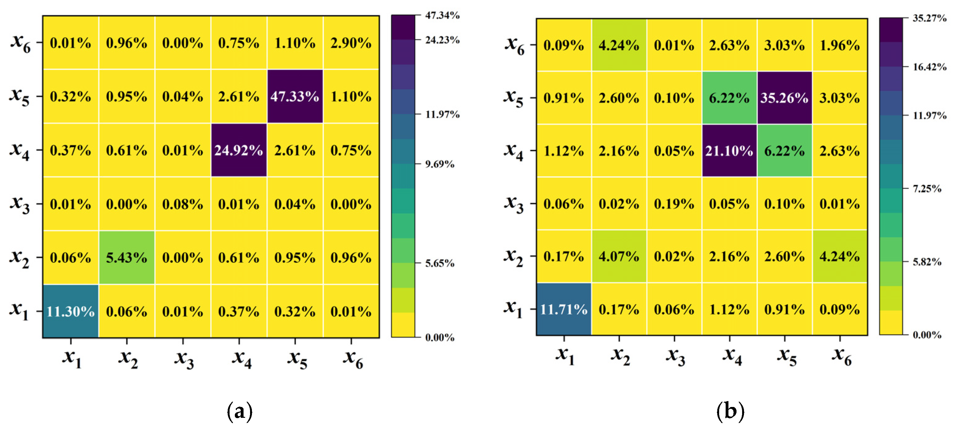
Figure 3 shows the sensitivity results for five scaling schemes. From Scaling 1 to Saling 5, as the scaling factor ${\beta }_i$ increases, the sensitivity indices of design variables change significantly. Among them, the main effect index of $x_1$ remains relatively unchanged, indicating minimal influence from the scaling variations, while the interaction effect index of $x_1$ increases. The main effect indices of $x_2$, $x_4$, $x_5$, and $x_6$ decrease, but the interaction effect indices between these design variables increase. Additionally, the importance ranking of design variables varies considerably across the five scaling schemes. In Scaling 1 and Scaling 3, the top two important design variables are $x_4$ and $x_5$. In Scaling 4, the top two important design variables are $x_5$ and $x_6$. In Scaling 5, the top two important design variables are $x_4$ and $x_6$.

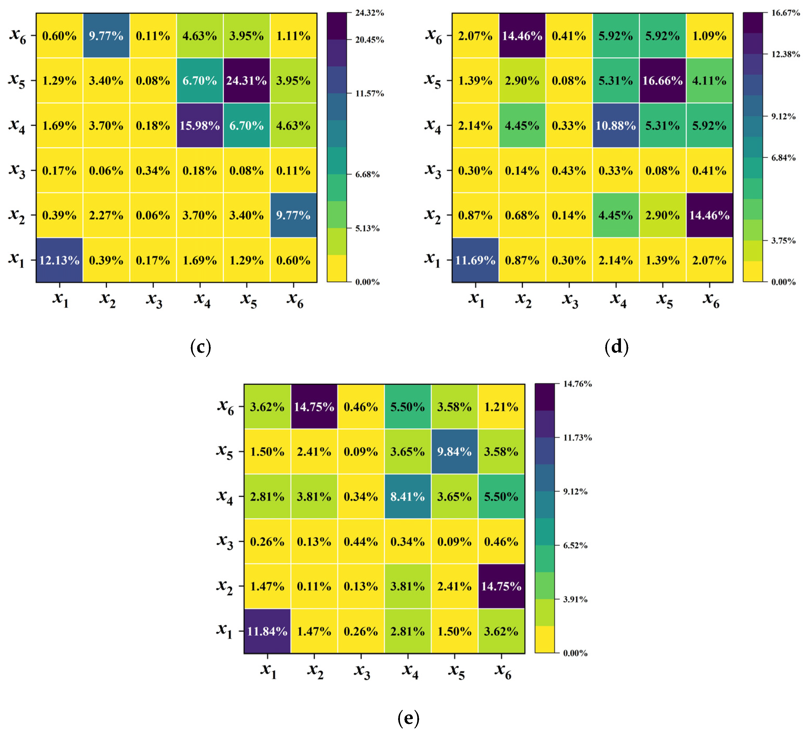
The sensitivity results for different translation schemes are shown in Figure 4. In Translation 1, $x_5$ and $x_6$ contribute the most to the objective function. Their interaction effect is relatively strong, with the interaction effect index exceeding 5%. In Translation 2, the main effect index of $x_6$ increases, while that of $x_5$ decreases. Additionally, the interaction effect between two variables weakens, with the interaction effect index falling below 1%. In Translation 3 and Translation 4, $x_4$ and $x_5$ contribute the most to the objective function. In Translation 5, both the main and interaction effect indices of $x_2$ increase significantly, making it the most influential variable.

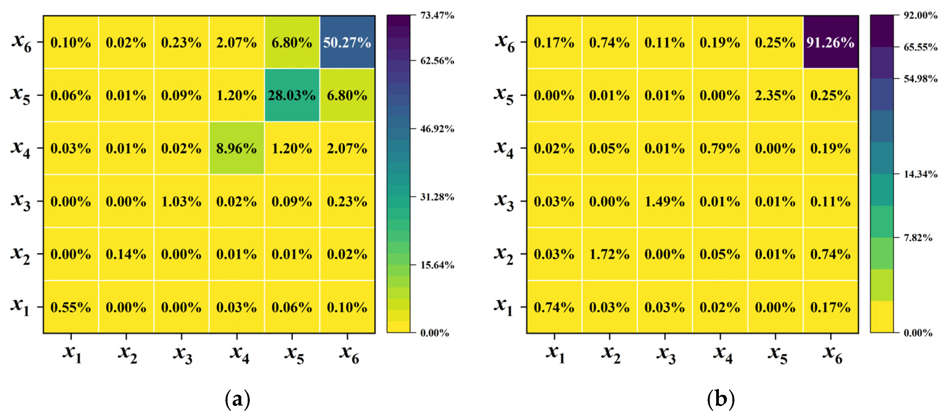
Figure 5 shows the sensitivity results for different combination schemes. In Combination 1 and Combination 2, the center position of the new design space coincides with the minimum point. In Combination 3 and Combination 4, the new design space does not contain the minimum point. In Combination 1 and Combination 2, it can be observed that as the scaling factor ${\beta }_i$ increases, the main effect index of the design variable $x_6$ decrease. However, it remains the most important design variable, with main effect index exceeding 50%. Additionally, the interaction effect index between design variables $x_5$ and $x_6$ increases significantly. In Combination 3 and Combination 4, when the new design space does not contain the minimum point, the sensitivity results vary significantly for different translation factor ${\alpha }_i$ under the same scaling factor ${\beta }_i$. In Combination 3, where the translation factor ${\alpha }_i=-2$ is used, $x_5$ and $x_6$ are the most important variables. In Combination 4, where a different translation factor ${\alpha }_i=2$ is applied, $x_5$ and $x_4$ becomes the most influential variables.

The function $f_2$ is a multi-extreme function with a relatively complex shape. The values of the function fluctuate greatly across different intervals, especially in regions containing local minima. Different variation schemes generate different design spaces, and the shape of the function within these design spaces can vary significantly. This leads to distinct, and, in some cases, even opposing sensitivity results.

In summary, whether dealing with single-extremum or multi-extremum functions, scaling, translation, and combination variations of the design space can significantly impact the sensitivity results of design variables. If the shape of the function changes notably within the design space, the sensitivity results may vary considerably. Therefore, it is crucial to carefully define the design space before conducting the sensitivity analysis.

5. A Wave Drag Reduction Case of NACA0012 Airfoil

5.1. Computational Fluid Dynamics Method and Verification

In this study, the aerodynamic performance of the airfoil is evaluated using an in-house structured CFD platform (Zhang et al., 2023). The Euler equations are applied for inviscid flow simulations, while the Reynolds-Averaged Navier–Stokes (RANS) equations are employed for viscous flows, with the $k-\omega$ model utilized for turbulence modeling. The fluid computational domain is discretized using the finite volume method. To ensure the reliability of the analysis, the accuracy of the CFD code has been validated. The aerodynamic performance of the RAE2822 airfoil is compared with the experimental and CFD solver employed in this study. Case 9 from the AGARD Report AR 138 is used for simulation under conditions $Ma=0.8$, $\alpha ={2.79}^{°}$, $\mathrm{Re}=6.5\times {10}^6$.

As shown in Figure 6, grid independence verification is achieved when the number of grids reaches 289 × 97, at which point the pressure coefficient and aerodynamic force of the airfoil become stable. The computational grid is C-grid, with the height of the first layer is $4\times {10}^{-6}$, and the total number of grid cells is 289 × 97. The pressure distribution of the RAE2822 airfoil, as depicted in Figure 7, shows great agreement between the CFD results and the experimental data, indicating the accuracy of the numerical simulation.

5.2. Problem Statement

Wave drag is the primary source of resistance in transonic flow. In this section, the problem of is studied. Using the NACA0012 airfoil as the baseline airfoil, this study analyzes the variations in wave drag sensitivity across different design spaces and investigates how these changes influence the wave drag of the transonic airfoil. The drag reduction problem is formulated as follows:

$$\mathrm{minimize} C_d$$

(37)

where $C_d$ is the drag coefficient. The calculation conditions are $Ma=0.8$, $\alpha =0^{\circ }$. The governing equation is the Euler equation. The structured computational mesh is generated by C-type topology, as shown in Figure 8. The design variables for the drag reduction problem are CST-parameterized variables. The NACA0012 airfoil is a symmetrical airfoil and has six CST-parameterized variables for both the upper and lower surfaces. Since the variables at the leading-edge of the upper and lower surfaces are opposites, only one variable is required to represent them. Thus, the total number of design variables is reduced to 11.

Taking the original design variable values of the NACA0012 airfoil, denoted as $x_{\mathrm{NACA}0012}$, as the center position of the initial design space, the size of the design space is defined as $r=\left|10\%\times x_{\mathrm{NACA}0012}\right|$. Therefore, the initial design space is expressed as $[x_{\mathrm{NACA}0012}-\left|10\%\times x_{\mathrm{NACA}0012}\right|,x_{\mathrm{NACA}0012}+\left|10\%\times x_{\mathrm{NACA}0012}\right|]$. In this drag reduction problem, since the minimum value of the objective function is unknown, only scaling and translation schemes are applied to the initial design space. The values of the scaling factor are presented in

Table 10. Parameter settings for the scaling scheme.

	Scaling 1	Scaling 2	Scaling 3
$\beta$	${\beta }_i=1$	${\beta }_i=1.5$	${\beta }_i=2$

, where Scaling 1 represents the initial design space.

Table 11. Parameter settings for the translation scheme.

	Translation 1	Translation 2	Translation 3
$\alpha$	${\alpha }_i=-1$	${\alpha }_i=0$	${\alpha }_i=1$

shows the values of the translation factor, where ${\alpha }_i=\pm 1$ indicates a translation amount one times the size of the initial design space, with the sign indicating the direction of the translation.

5.3. Definition of Shock-Wave Strength

The magnitude of shock-wave drag is directly correlated with the strength of the shock-wave. To better describe changes in the shock-wave strength, the decrease in pressure coefficient between the two sides of the shock wave, denoted as $\mathrm{\Delta }{C}_p$, is introduced. The expression for $\mathrm{\Delta }{C}_p$ is defined as follows:

$$\mathrm{\Delta }{C}_p=C_{p_2}-C_{p_1}={\displaystyle \frac{\mathrm{\Delta }p}{\frac{1}{2}{\rho }_{\infty }{V}_{\infty }^2}}$$

(38)

where, $C_{p_1}$ is the pressure coefficient at the wave front, $C_{p_2}$ is the pressure coefficient at the wave back, $\mathrm{\Delta }p$ is the pressure decrease between the two sides of the shock wave, ${\rho }_{\infty }$ is the freestream density, $V_{\infty }$ is the freestream velocity.

By the energy conservation equation for one-dimensional inviscid flow and the isentropic relation [34,35,36], it can be expressed as follows:

$$p_1={\left[{\displaystyle \frac{\left.M_{\infty }^2\cdot \gamma (\gamma -1\right)+2\gamma }{M_1^r\cdot \gamma (\gamma -1)+2\gamma }}\right]}^{{\displaystyle \frac{\gamma }{\gamma -1}}}\cdot p_{\infty }$$

(39)

where, $p_1$ is the static pressure at the wave front, $M_1$ is the Mach number at the wave front, $\gamma$ is the specific heat ratio, $p_{\infty }$ is the freestream static pressure, $M_{\infty }$ is the freestream Mach number.

Based on the static pressure relationship between the two sides of the shock wave:

$${\displaystyle \frac{p_2}{p_1}}={\displaystyle \frac{2\gamma M_1^2-(\gamma -1)}{\gamma +1}}$$

(40)

where $p_2$ is the static pressure at the wave back.

Therefore,

$$\mathrm{\Delta }p=p_2-p_1={\displaystyle \frac{2\gamma M_1^2-2\gamma }{\gamma +1}}{p}_1$$

(41)

Substituting Equations (39) and (41) into Equation (38) yields

$$\mathrm{\Delta }{C}_p={\displaystyle \frac{4(M_1^2-1)}{\gamma +1}}\cdot {\displaystyle \frac{1}{M_{\infty }^2}}\cdot {[{\displaystyle \frac{(\gamma -1)M_{\infty }^2+2}{(\gamma -1)(M_1^2-1)+\gamma +1}}]}^{{\displaystyle \frac{\gamma }{\gamma -1}}}$$

(42)

5.4. Effect of Design Space Variation on Sensitivity Results of the Drag Coefficient

5.4.1. Effect of Scaling Variation on Sensitivity Results

The sensitivity results for the drag coefficient under different scaling schemes (only results with sensitivity indices greater than 1% are depicted) are shown in Figure 9. In Scaling 1, $x_1$, $x_2$, and $x_7$ contribute the most to the drag coefficient, with their main effect indices exceeding 20%. Followed by $x_3$ and $x_8$, with main effect indices of 4.499% and 4.51%, respectively. In contrast, the main effect indices of other variables, namely $x_4$, $x_5$, $x_9$, and $x_{10}$ are less than 2%, indicating that they have little effect on the drag coefficient. As the scaling factor ${\beta }_i$ increases, the main effect indices of $x_1$ rises, while those of $x_2$ and $x_7$ decline. Additionally, the main effect indices of other design variables exhibit relatively minor changes. In Scaling 3, $x_7$ emerges as the most significant variables for the drag coefficient, followed by $x_2$. Under all three scaling schemes, $x_1$, $x_2$, and $x_7$ remain the primary contributors to the drag coefficient, although their contribution rankings differ slightly across the different schemes. Furthermore, it is observed that the sensitivity results for the upper and lower surfaces are symmetrical. For example, $x_2$ and $x_7$, as well as $x_3$ and $x_8$, exhibit similar behavior.

To further verify the accuracy and reliability of sensitivity results, perturbations are applied to important and unimportant design variables in each scheme. The design variables with sensitivity indices ranking in the top two are defined as important design variables, while those ranking in the bottom two are defined as unimportant design variables. For Scaling 1, the important variables are $x_2$ and $x_7$, and the unimportant variables are $x_4$ and $x_9$; For Scaling 2, the important variables are $x_2$ and $x_7$, and the unimportant design variables are $x_4$ and $x_9$; For Scaling 3, the important variables are $x_2$ and $x_7$, and the unimportant design variables are $x_4$ and $x_9$.

Positive perturbations are applied only to specified variables (an increase in the absolute value of the variable is defined as a positive perturbation), and the perturbation is set to $\left|10\%\times x_{\mathrm{NACA}0012}\right|$. The other variables remain at their original values. Since the important and unimportant variables is consistent across all three schemes, we chose Scaling 1 for the perturbation analysis. As shown in

Table 12. Comparison of the drag coefficient under different perturbations.

	NAC0012 (Baseline)	Scaling 1
		Important	Unimportant
$C_d$	0.0093	0.0142	0.0097
		(+52.69%)	(+4.30%)
$\mathrm{\Delta }{C}_p$	0.8136	0.9013	0.8207
		(+10.78%)	(+0.87%)

. It is evident that, compared to the baseline airfoil, the drag coefficient increases by 52.69% and $\mathrm{\Delta }{C}_p$ increases by 10.78% when the important variables are perturbed. In contrast, when the unimportant variables are perturbed, the drag coefficient only increases by 4.30% and $\mathrm{\Delta }{C}_p$ increases by 0.87%. Perturbations in the important design variables have a more substantial impact on the drag coefficient, whereas perturbations in the unimportant design variables have negligible effects. This outcome is consistent with sensitivity analysis results.

Figure 10 and Figure 11 illustrate the pressure and Mach number distributions under different perturbations. Compared to the baseline airfoil, the shock wave on the perturbed airfoils shifts rearward to nearly the same position. Perturbations in important variables significantly increase the shock-wave strength, while perturbations in unimportant variables have a much smaller impact. These results are consistent with the sensitivity analysis results.

5.4.2. Effect of Translation Variation on Sensitivity Results

Figure 12 shows the sensitivity results for the drag coefficient under different translation schemes (only results with sensitivity indices greater than 1% are depicted). The sensitivity indices of the design variables differ significantly across the three translation schemes, and the importance ranking of the design variables for the drag coefficient changes accordingly. For Translation 1, the important variables are $x_7$ and $x_8$, with main effect indices 51.185% and 33.205%, respectively, and the unimportant variables are $x_4$ and $x_6$; For Translation 2, the important design variables are $x_2$ and $x_7$, with main effect indices 30.343% and 29.983%, respectively, and the unimportant design variables are $x_4$ and $x_9$; For Translation 3, the important design variables are $x_1$ and $x_2$, with main effect indices 33.677% and 41.694%, respectively, and the unimportant design variables are $x_7$ and $x_9$.

Perturbations are applied only to important and unimportant variables in each scheme, with the perturbation magnitude set to $\left|10\%\times c^{new}\right|$, while the other variables remain at their original values.

Table 13. Comparison of the drag coefficient under different perturbations.

		${\mathit{C}}_{\mathit{d}}$	$\mathbf{\Delta }{\mathit{C}}_{\mathit{p}}$ (Upper Surface)	$\mathbf{\Delta }{\mathit{C}}_{\mathit{p}}$ (Lower Surface)
Translation 1	Baseline	0.0142	0.0379	0.8771
	Important	0.0194 (+36.62%)	0.0382 (+0.79%)	1.1423 (+30.24%)
	Unimportant	0.0145 (+2.11%)	0.0398 (+5.01%)	0.9270 (+5.69%)
Translation 2	Baseline	0.0093	0.8136	0.8136
	Important	0.0142 (+52.69%)	0.9013 (+10.78%)	0.9013 (+10.78%)
	Unimportant	0.0097 (+4.30%)	0.8207 (+0.87%)	0.8207 (+0.87%)
Translation 3	Baseline	0.0142	0.7952	0.0406
	Important	0.0231 (+62.68%)	0.9867 (+24.08%)	0.0556 (+36.95%)
	Unimportant	0.0149 (+4.93%)	0.8028 (+0.09%)	0.0386 (−9.11%)

shows the drag coefficient and $\mathrm{\Delta }{C}_p$ of both perturbed airfoils and baseline airfoils. The corresponding pressure and Mach number distributions are shown in Figure 13 and Figure 14. A distinct difference can be observed in the shove-wave region of perturbed airfoils compared to the baseline. The specific comparisons are as follows:

(1)

Translation 1: For the upper surface, the shock wave shows almost no change when the important variables are perturbed. However, when unimportant variables are perturbed, the shock wave moves rearward with a slight increase in strength. For the lower surface, the shock wave on the perturbed airfoils shifts rearward, and its strength increases significantly when the important variables are perturbed. Overall, the drag coefficient increases by 36.62% in important variables, while it only increases by 2.11% with perturbations in unimportant variables.

(2)

Translation 2: The areas of the shock-wave region on the upper and lower surfaces are nearly the same. Perturbations in important variables result in a 52.69% increase in the drag coefficient and a 10.78% increase in $\mathrm{\Delta }{C}_p$. In contrast, when unimportant variables are perturbed, the drag coefficient increases by only 4.30%, and $\mathrm{\Delta }{C}_p$ only increases by 0.87%.

(3)

Translation 3: On the upper surface, the shock-wave strength is significantly enhanced by perturbations in important variables, with little change when unimportant design variables are perturbed. On the lower surface, the shock-wave strength decreases with perturbations in unimportant variables but increases when important variables are perturbed. Overall, the drag coefficient increases by 62.68% when important variables are perturbed, whereas it increases by only 4.93% when unimportant variables are perturbed.

As the design space changes, the sensitivity results of design variables are affected, with the shock wave being a primary factor influencing these changes. To further explore the impact of design space variations on the shock wave, uniform sampling is conducted within different design spaces. Figure 15 illustrates the relationship between shock-wave strength, position, and design space. When the design space expands in the positive direction, the shock-wave strength increases, and its position shifts rearward. Conversely, as the design space expands in the negative direction, the shock-wave strength decreases, and the shock-wave position shifts forward.

The sensitivity results of the scaling and translation schemes reveal that the contributions of geometric parameterized variables to the drag coefficient vary across different design spaces. Variations in the design space directly influence the sensitivity indices of variables, which in turn affect their importance ranking. An analysis of pressure and Mach number distributions shows that variations in the design space primarily affect the shock-wave position and strength, thereby altering the sensitivity indices of the geometric parameterized variables.

5.5. Effect of Design Space Variation on Sensitivity Analysis at Different Mach Numbers

To further investigate the influence of design space variations on the sensitivity results of drag coefficient, particularly in scenarios with or without a shock wave, a case without a shock wave is selected for comparison in this subsection. The calculation conditions are $Ma=0.6$, $\alpha =0^{\circ }$. All other settings are identical to those in Section 5.2.

Figure 16 presents the sensitivity analysis results for the drag coefficient under different scaling schemes. Across the three scaling schemes, it is evident that when no shock wave is generated on the airfoil surface, $x_1$ is the most important variable for the drag coefficient, with main effect indices exceeding 95%. In contrast, the main effect indices of other variables are all less than 1% and can be ignored. There are notable differences between cases with shock waves and without shock waves. When a shock wave is generated on the airfoil surface, $x_2$ and $x_7$ become more influential variables for the drag coefficient.

Figure 17 presents the sensitivity analysis results for the drag coefficient under different translation schemes. It can be observed that the sensitivity results obtained from different translation schemes are essentially the same. $x_1$ is the most important variable for the drag coefficient, while the contributions of other variables are minimal. This outcome differs from the sensitivity results obtained in Section 5.3.

Comparing the sensitivity results under two Mach numbers, it can be seen that the sensitivity results of the drag coefficient in different design spaces are related to the flow conditions, which directly affect the importance ranking of the geometric parameterized variables. From the sensitivity indices of these variables, it is clear that when a shock wave is present on the airfoil surface, the influence of the geometric parameterized variables on the drag coefficient becomes more complicated.

6. Conclusions

This paper investigates the influence of geometric parameterized variables on transonic flow fields under different design spaces. Three variation schemes of the design space are established in this study, and their effects on sensitivity results are analyzed using two test functions and a wave drag reduction case. The underlying causes of these patterns are also explored. The conclusions are as follows:

(1) In the test functions, variations in the design space (scaling, translation, and combination) have a significant impact on the sensitivity results. The trends of sensitivity indices for these variables are directly influenced by the shape of functions within the design space.

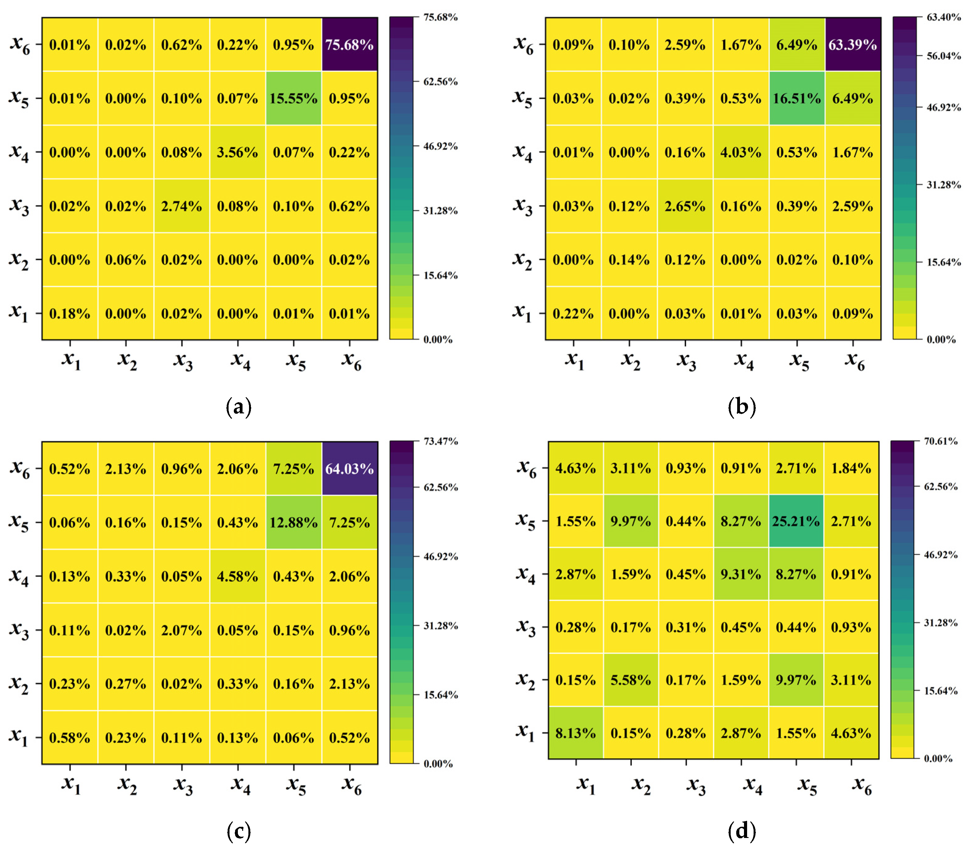
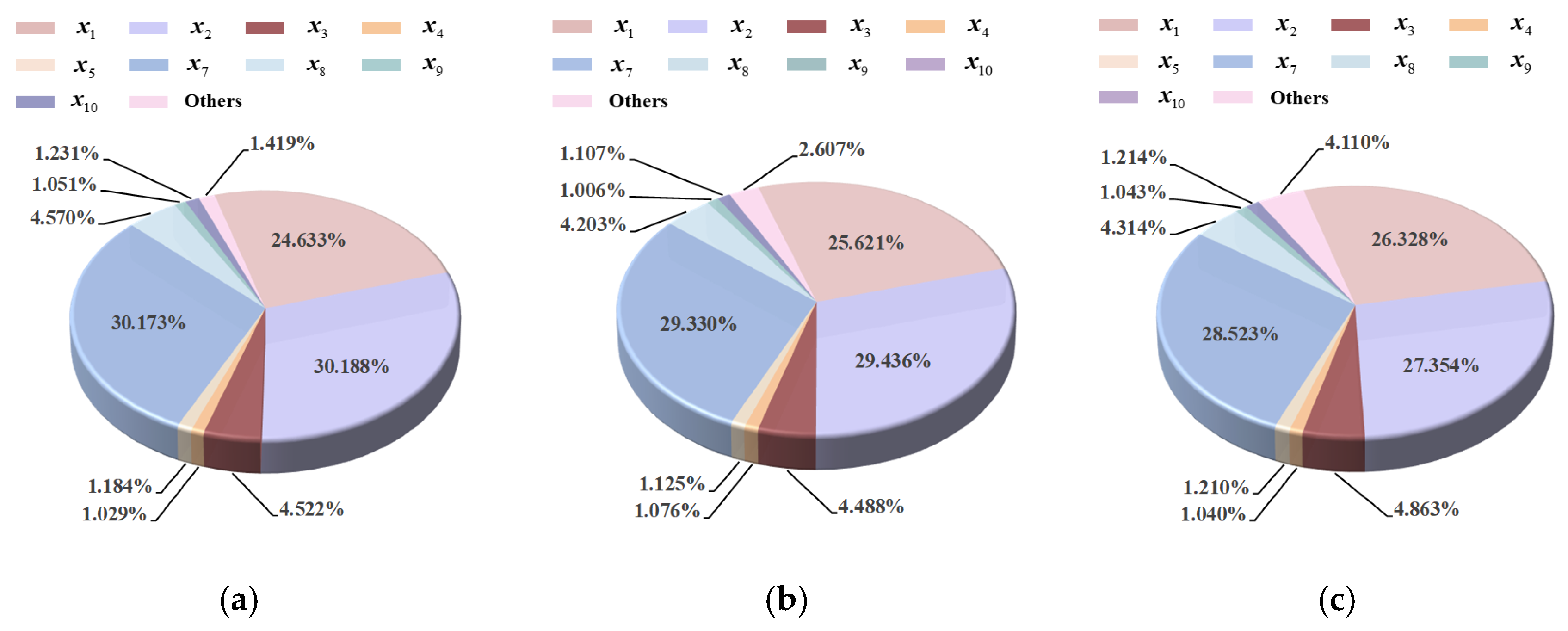
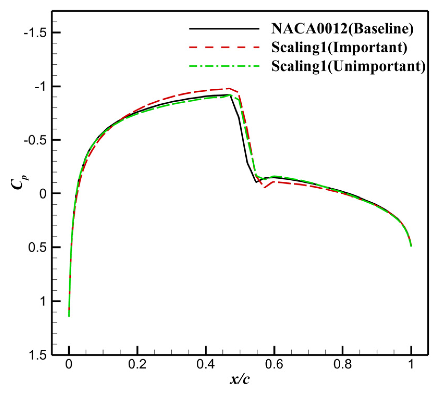
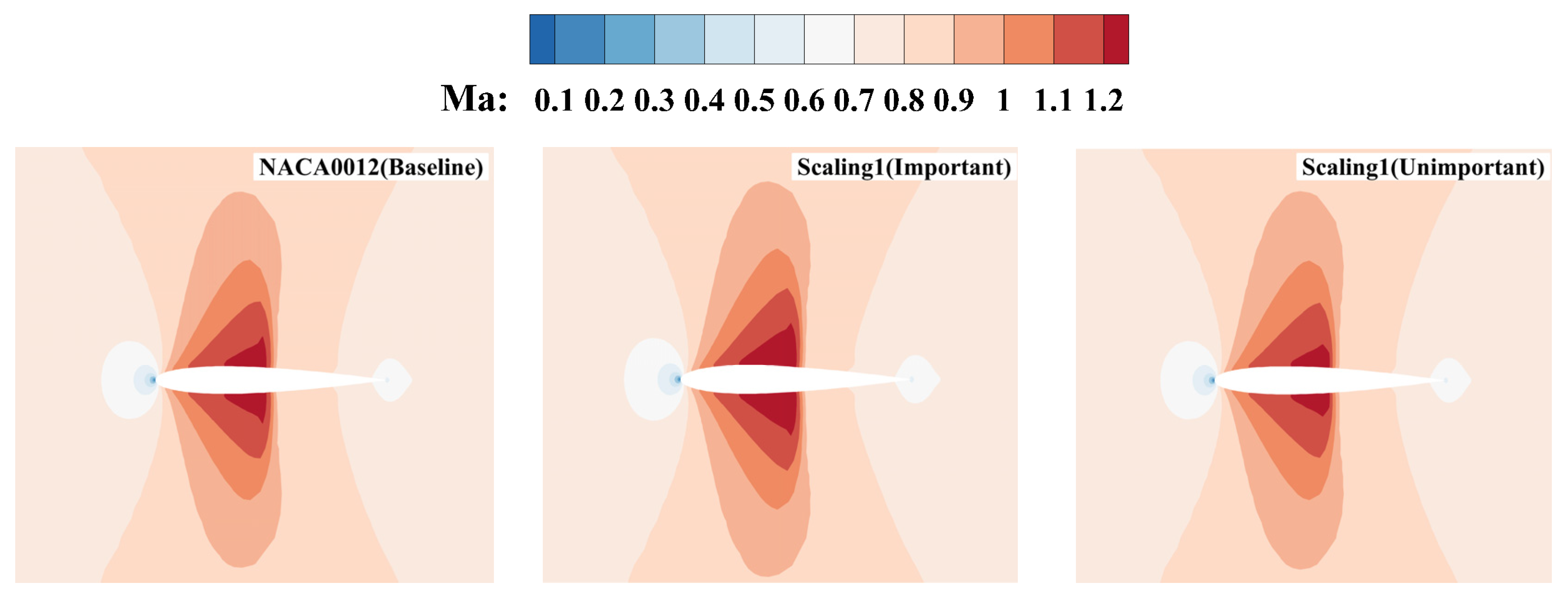
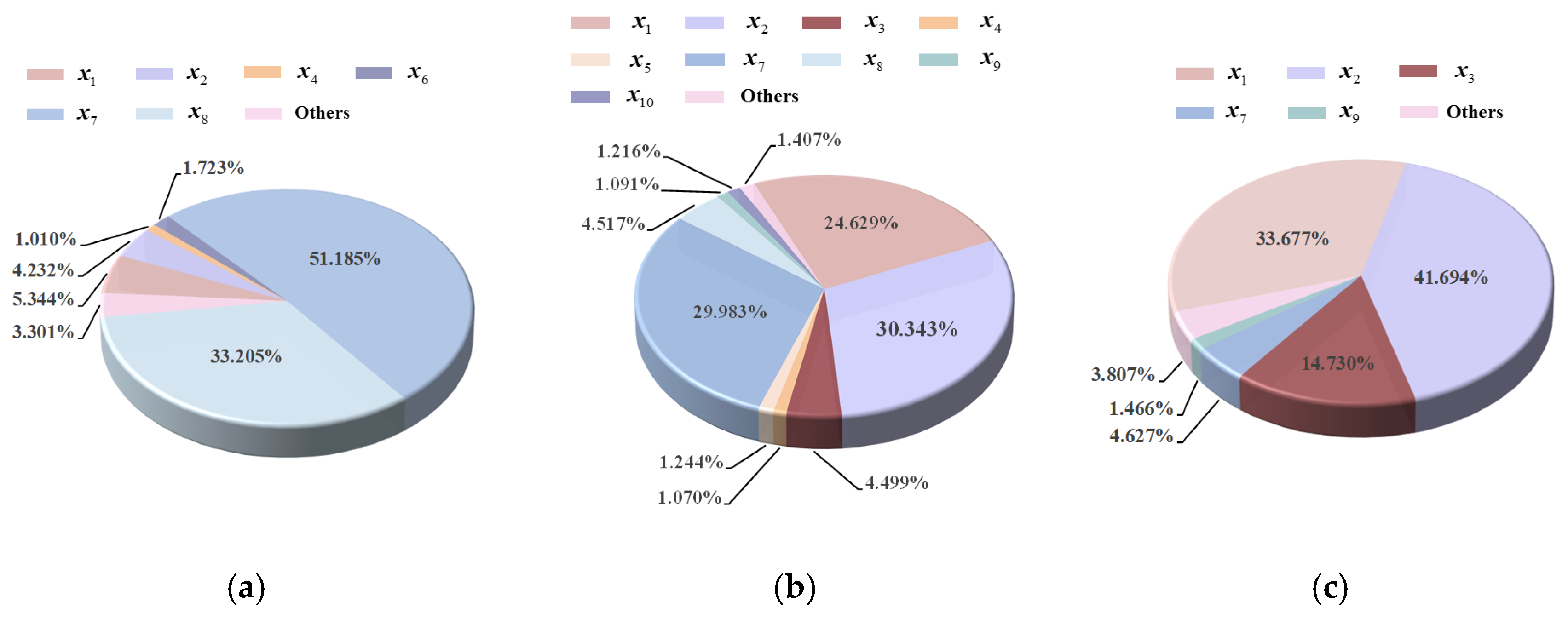
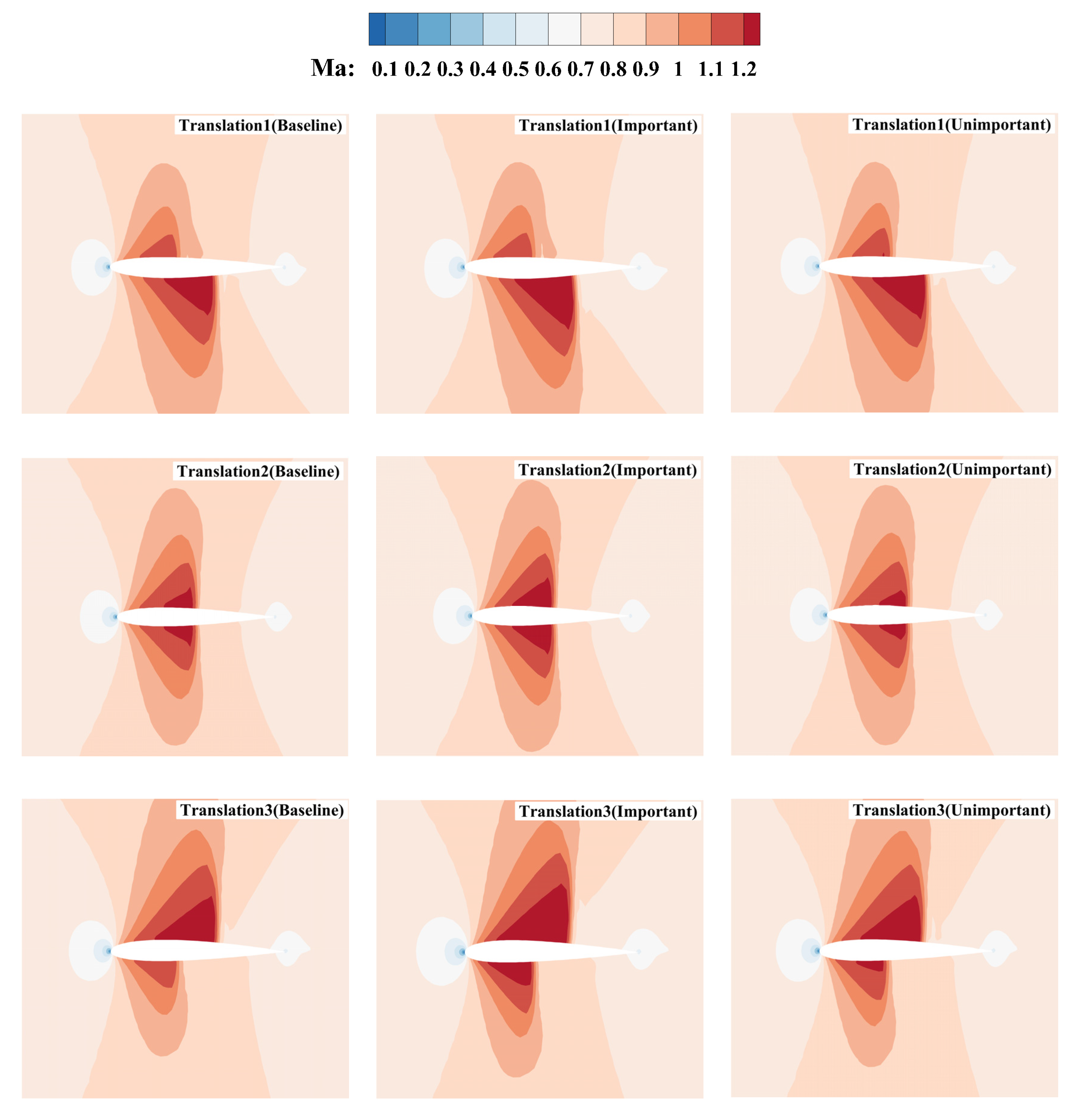
(2) In the wave drag reduction case, variations in the design space affect the relationship between geometric parameterized variables and the flow field, specifically influencing the shock-wave position and strength, which is reflected in the sensitivity indices of the variables.

(3) The sensitivity indices of geometric parameterized variables are closely related to the Mach number. As the Mach number changes, the sensitivity results of these variables in different design spaces also change accordingly.

(4) The conclusions of this paper have important implications for aerodynamic optimization design. When performing the sensitivity analysis method in the optimization design, careful selection of the design space is crucial to ensure accurate results.