Temperature Prediction for Aerospace Thermal Tests Based on Physical and LSTM Hybrid Model

Abstract

During spacecraft operations, structures experience extreme aerodynamic heating, necessitating thermal testing to gather data on the thermal response of surface materials. Given the nonrepeatable nature of these test articles, accurately predicting the temperature rise profile under thermal load inputs is essential before formal testing. Although theoretical analyses can develop precise internal heat transfer models for modules, limited test data hampers the modeling of inter-module heat transfer processes. Furthermore, variations in test article parameters across different tests restrict the generalizability of existing models. We present a hybrid modeling approach that integrates a physical model with a long short-term memory (LSTM) network to address these challenges. The LSTM model is trained on historical data to capture complex inter-module heat transfer dynamics. Additionally, varying parameters of the test articles are included as model inputs to enhance versatility and adaptability. Experiments demonstrate that the model achieves high prediction accuracy (MAE = 17.41 (K) R² = 0.9988) even when test article parameters differ from historical data. Moreover, it shows strong adaptability to changes in the input power signal (MAE = 34.91 (K) R² = 0.9990). This study successfully predicts temperature profiles during thermal testing using minimal test data, thereby improving computational efficiency and reducing testing costs, which facilitates the effective implementation of formal thermal testing.

1. Introduction

When a spacecraft crosses the Earth’s atmosphere or a high-speed vehicle cruises through the atmosphere, it not only experiences a mechanical environment consisting of various mechanical loads such as aerodynamic forces, vibration, noise, inertial forces, etc., but also faces a severe aerodynamic thermal environment [1]. These thermal energies heat critical areas, such as large thermal structures and wing leading edges, which can cause the local temperature of the vehicle structure to exceed 2000 °C [2]. This harsh thermal environment can have a series of adverse effects on the structural material properties and internal and external components of the vehicle. The normal operation of spacecraft can be significantly impacted, potentially leading to catastrophic events such as disintegration. On 1 February 2003, during the Space Shuttle Columbia’s reentry into the atmosphere, the spacecraft experienced intense aerodynamic heating on its surface, with temperatures exceeding 1649 °C. This extreme heat caused the landing gears to melt and eroded the heat-insulating tiles, ultimately destabilizing the spacecraft and leading to its destruction [3]. Therefore, aerospace structural thermal tests are particularly critical in the design process of supersonic vehicles, taking into account the aerodynamic thermal problems and the need to obtain the thermal response signals of surface materials and analyze their properties [4].

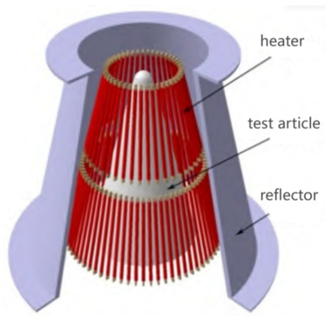
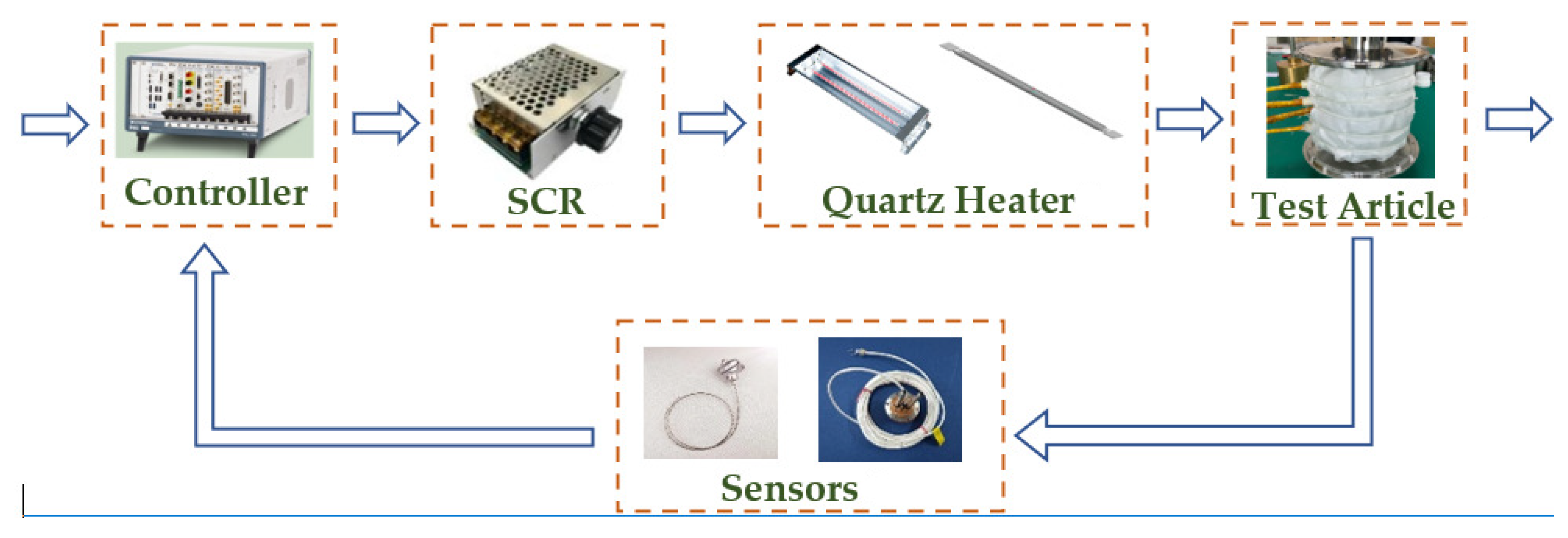
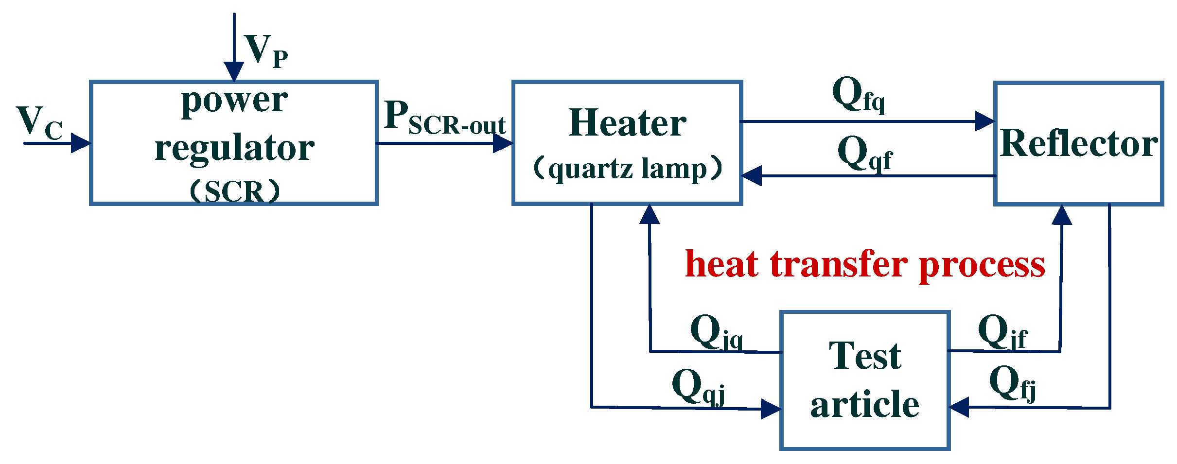
Due to the irreversible changes in the test article’s physical properties that may occur after it has been subjected to high-temperature heating, using this article for further testing may result in significant deviations. Therefore, most thermal tests for aerospace structures involve one-time test articles, making it crucial to implement predictions to enhance accuracy and reduce costs. Developing models to forecast the temperature of test articles is essential. Traditional thermal test system models, based on physics and parameter identification, play a vital role in temperature prediction. Cui et al. [5] examined the power characteristics, amplification factors, and time constants of quartz lamp heaters using both theoretical and experimental methods, contributing valuable data for temperature model establishment. Zhang et al. [6] investigated the dynamic characteristics of thyristor power regulation devices and quartz lamp heaters, applying system identification techniques to enhance the mathematical models of various thermal test system modules. He et al. [7] created a mathematical model for the temperature control system of an aircraft’s hot and cold airflow mixing chamber using physical modeling methods, along with a controlled autoregressive moving average model for offline identification of heater system parameters, resulting in a more accurate model. While physical modeling has clarified parameters affecting hysteresis, little research has explored the combined effects of design parameters like size and material properties on temperature coefficients [8]. In aerospace structural thermal testing, obtaining valid model information is challenging due to confidentiality concerns. Additionally, physics-based models require precise input data, are complex and time-consuming to compute, and the one-time nature of thermal tests limits the availability of data for model parameter identification. This complicates the establishment of accurate physical models, thereby affecting temperature prediction accuracy.

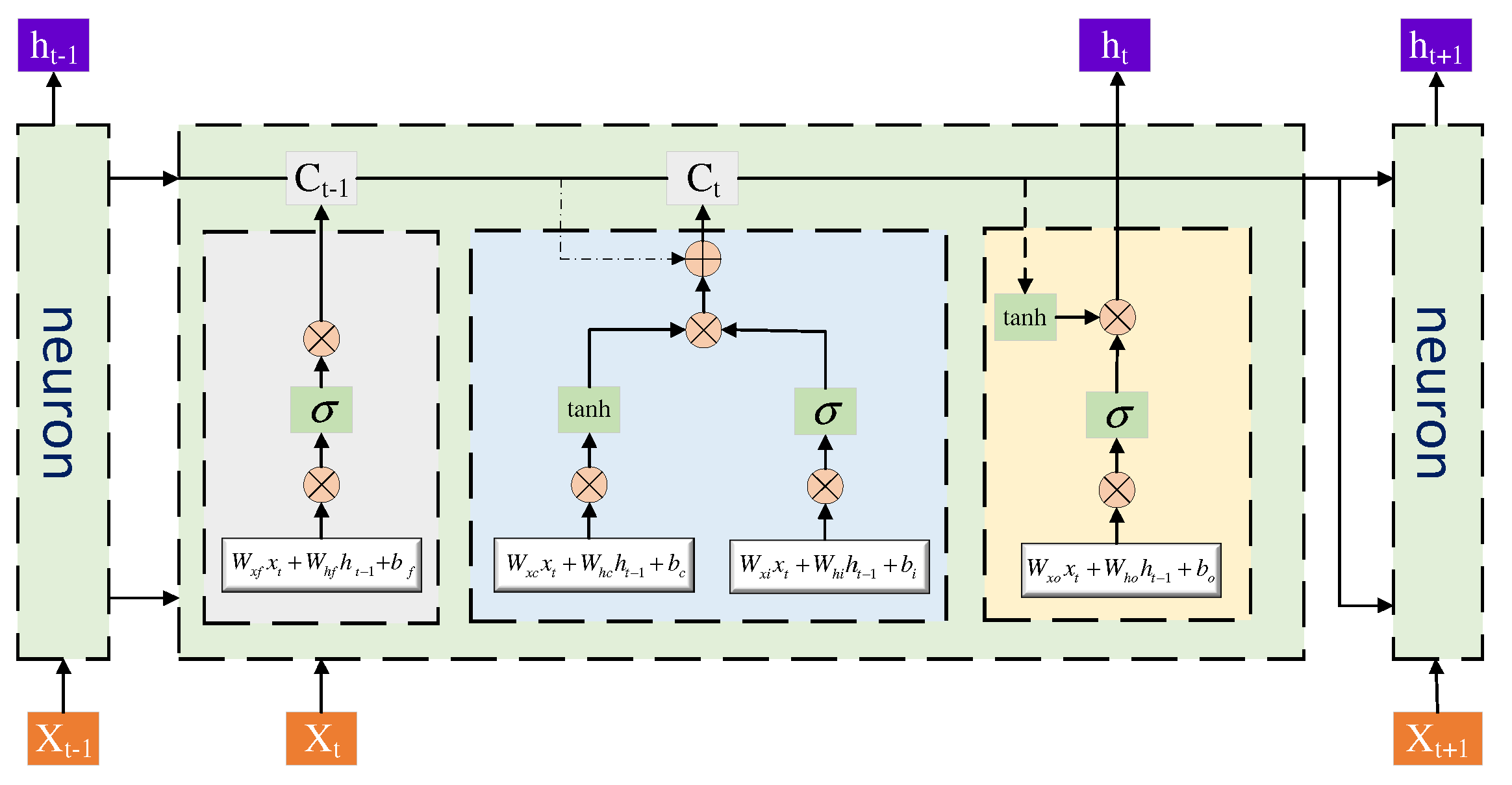
In recent years, deep learning has emerged as a key technology in advanced artificial intelligence, utilizing multilayered architectures to automatically extract high-level abstract features from data [9]. This approach does not rely on manual design. Leveraging these advantages, deep learning models have achieved significant success in various time series forecasting tasks, including remote sensing [10] and multisensor data fusion [11]. They have also proven effective in uncovering complex relationships among multiple time series [12]. Jun et al. [13] combined traditional physics-based model outputs with historical data to train long short-term memory (LSTM) networks for flood trend forecasting, enhancing prediction accuracy while reducing reliance on experimental data and improving computational efficiency. A deep learning approach using self-organizing maps (SOMs) and multilayer perceptrons (MLPs) for multisensor data prediction was proposed in [14]. Reference [15] introduced a deep architecture for traffic flow prediction that employed stacked autoencoders and a logistic regression layer. Additionally, Reference [16] discussed a forecasting model for solar power generation utilizing autoencoders and LSTM with various activation functions. Fang et al. [17] developed a temperature-strain mapping model based on transfer learning and a bidirectional LSTM network, employing analytical modal decomposition to denoise strain data, training the LSTM on this dataset, and transferring parameters to other datasets. However, this purely data-driven approach can diverge from physical mechanisms [18]. While aerospace thermal tests provide substantial historical data for model training, the model complexity increases with various inputs, including geometric and physical parameters of heaters and test articles. This complexity results in significant computational demands during training, raising the risk of model overfitting. Furthermore, the lack of interpretability in trained models complicates the identification of potential issues during the prediction process.

Model–data fusion is an integrated approach designed to enhance predictive capabilities and deepen the understanding of complex systems by combining historical data with theoretical models or computational simulations [18]. Ni et al. [19] introduced a physics-informed residual network that integrates physical principles into the learning process to improve the accuracy of bearing diagnostics under non-steady-state conditions. Grover et al. 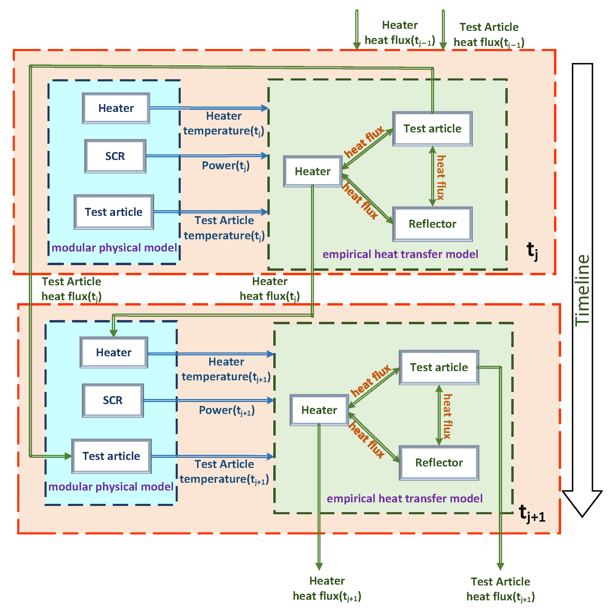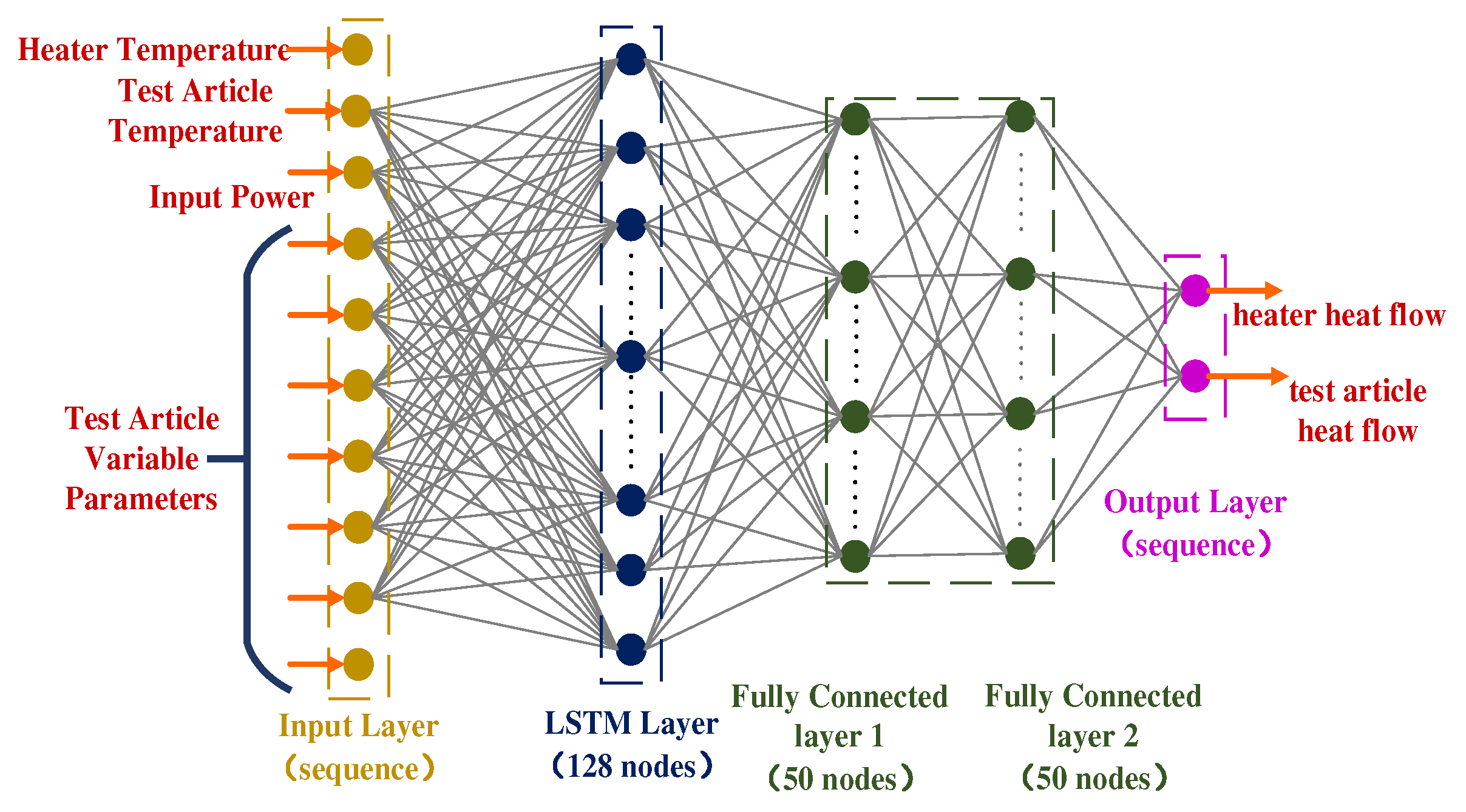[20] proposed a hybrid method that merges trained predictive models with deep neural networks to calculate the joint statistics of various weather-related variables. To address the limitations of both physical modeling and machine learning modeling, and to tackle the critical challenges of data scarcity and insufficient model information in temperature predictions for thermal test systems, we introduce a hybrid modeling framework. This framework effectively integrates the ease of application and interpretability of physics-based models with the dynamic capabilities of LSTM networks and exhibits strong extrapolation, transfer, and generalization abilities.

The methodology is grounded in the theoretical construction of physical models for various modules within the thermal test system, coupled with developing a complex heat transfer process model utilizing the LSTM network. This method facilitates the synergistic integration of the two models, enhancing the interpretability of the LSTM network by leveraging the strong interpretability of the physical model. Additionally, the incorporation of the LSTM network reduces the modeling complexity of the aerospace thermal test system. After testing and analyzing the results, this approach demonstrates the ability to accurately predict the temperature of the test articles and adjust the control parameters during the thermal test, thereby preventing potential damage to the test articles caused by inadequate control parameters in the formal test. Furthermore, this method offers a promising solution for specific engineering applications characterized by data scarcity, high computational demands, and modeling challenges. The main contributions of this study include:

(1)

A high-accuracy thermal test temperature prediction method is proposed, which can achieve precise temperature prediction based on a limited amount of experimental data, thereby providing correct guidance for formal thermal tests.

(2)

The temperature prediction method proposed in this study demonstrates significant generality and generalization capability when dealing with variations in test article parameters across different thermal tests. This avoids the need for remodeling for each new test article, improving computational efficiency and reducing test costs.

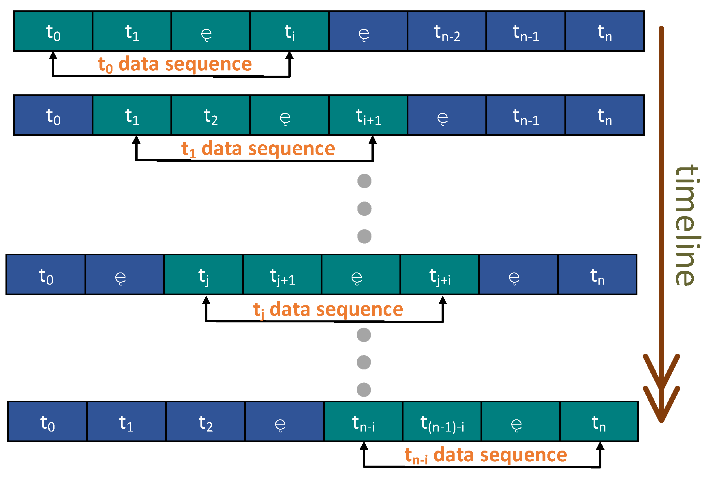
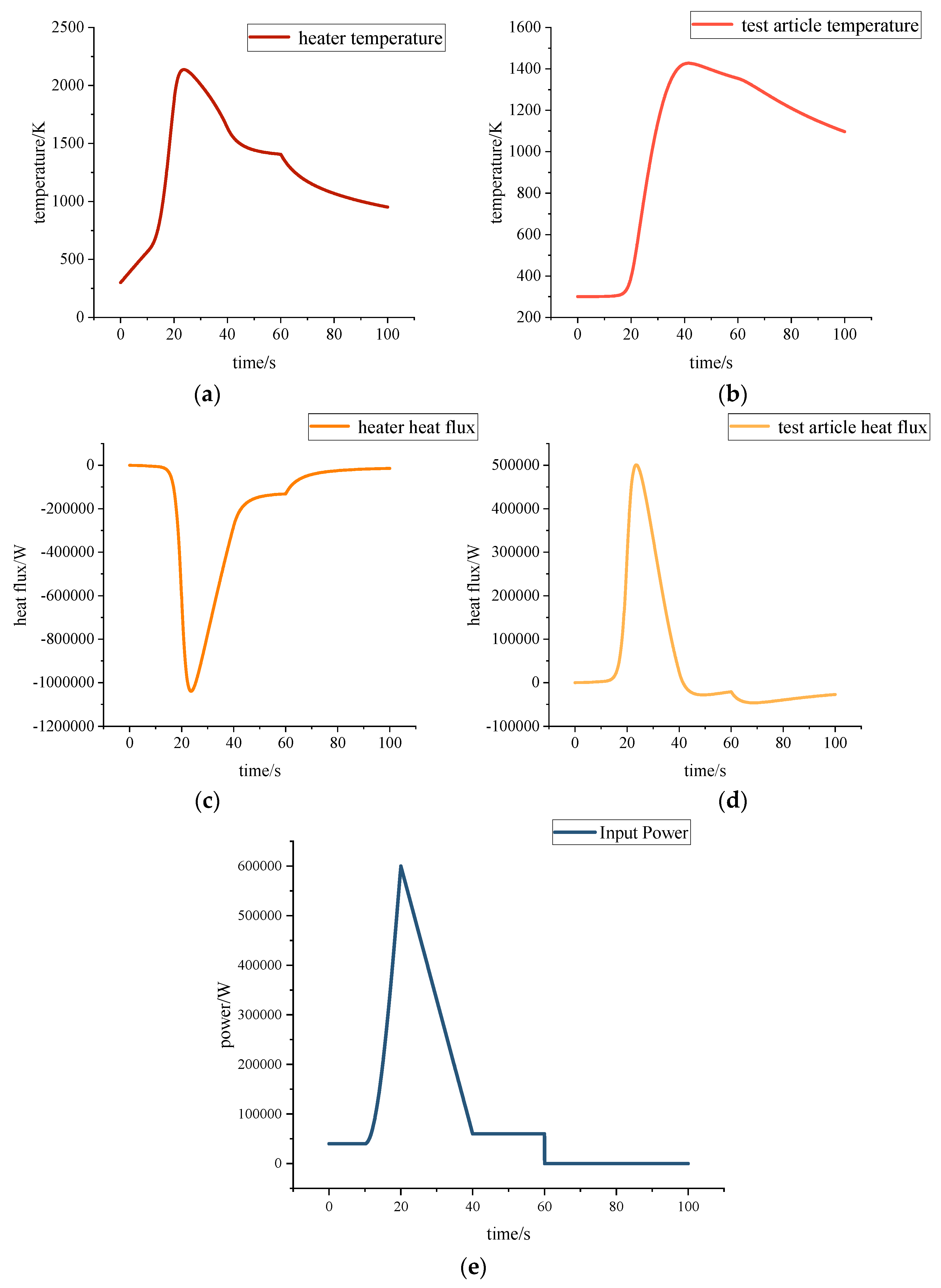
The remainder of this paper is organized as follows. In Section 2, we detail the physical models of the various modules of the thermal test system. In Section 3, we present the prediction method of the hybrid physical–LSTM model, including the structure of the LSTM model and the prediction procedure. In Section 4, we compare the observed values with the predictions made by the standalone LSTM model and the hybrid model. In Section 5, we provide the conclusions of this study.

2. Thermal Test System Model

2.1. Aerospace Thermal Test System

The heating methods are constrained by the structural, material, and design verification requirements of the spacecraft, mainly including radiant heating, convective heating, and conductive heating, as well as other advanced technologies such as induction heating, electron beam heating, and laser heating. Arc-heating wind tunnels and high-temperature nozzles achieve convective heat transfer through high-temperature and high-speed airflow, while rocket sleds utilize aerodynamic heating generated by speed, making them an ideal thermal simulation method. Conductive heating is typically implemented using heating pads or through electrical conduction, serving a relatively singular purpose. In contrast, radiant heating commonly employs quartz lamp arrays or graphite strip heaters, which are favored for their small size, high power, adjustability, and stability, making them suitable for complex structures. With the continuous increase in testing temperature and heating power density requirements—for instance, the maximum heating capability of graphite heaters developed for the Space Shuttle and hypersonic vehicles in the United States can reach 5600 kW/m²—similar technological advancements have been achieved domestically with modular quartz lamp heating devices [21,22,23,24,25,26,27,28]. Figure 1 illustrates the conical thermal test device used in the radiant heating tests of a spacecraft’s antenna cover [29].

The heating system for thermal tests consists of heaters, power regulation devices, sensors, and control equipment, forming a closed-loop control system together with the test article. The control equipment typically comprises a programmable logic controller (PLC), a digital signal processor (DSP), or a computer. The power regulation device employs a silicon controlled rectifier (SCR), while the heater is usually selected from quartz lamp arrays or graphite heaters. Sensors used in the system include heat flux sensors or temperature sensors. The heated structural components can be complete tactical or launch models, or they may consist of partial components of the model [30].

During the heating process, the heat flux or temperature data of the test article’s surface, absorbed in real-time, is collected via heat flux sensors or temperature sensors. This data is then compared and computed against the target value, generating output commands for the controller, which are subsequently transmitted to the power regulation device. In the heating process control system, the primary function is to adjust the voltage and linearly amplify the controller’s output, thereby changing the input power to the heater and subsequently altering the thermal energy delivered to the test article. This process ultimately ensures that the thermal state of the test article’s surface follows the specified control target curve, achieving automated heating control. The thermal energy absorbed by the structural surface can be directly represented as heat flux density or indicated by the temperature rise state of the structural wall after absorbing heat. The specific workflow of the thermal test system is illustrated in Figure 2.

2.2. Mechanistic Model

We focus on the modeling and temperature prediction of test systems in hydrostatic tests. Due to the high accuracy and minimal time delay of the heat flow and temperature sensors employed in this study, the sensors’ dynamic behavior is assumed to be negligible in the modeling process. This assumption effectively simplifies the model’s complexity without compromising the accuracy of the temperature prediction results. The block diagram of the physical model for the thermal test system is presented in Figure 3, with the parameter information detailed in

Table 1. Meaning of names in the mechanism model of the thermal test system.

Symbol	Interpretations	Symbol	Interpretations
VC	The control voltage output from the controller	Qfq	Heat flow radiated to the heater by the reflector
VP	Power input AC voltage	Qqf	Heat flow radiated from the heater to the reflector
PSCR-out	SCR output power	Qqj	Heat flow radiated by the heater to the test article
Qfj	Heat flow radiated from the reflector to the test article	Qjq	Heat flow radiated from the test article to the heater
Qjf	Heat flow radiated by the test article to the reflector

.

2.2.1. Physical Model of SCR

In thermal testing, the power supply provides the necessary energy support, typically utilizing an easy-to-use AC power source accompanied by a voltage regulation device, such as an AC/AC converter based on thyristor technology. This device adjusts the voltage through the use of thyristors, transformers, and control circuits. The input AC power is rectified and stepped down before the output voltage is managed by triggering the thyristors using control signals. Research has shown that the amplification factor of thyristor devices decreases as the input voltage increases, and the static functional relationship between input and output voltages remains fixed.

As illustrated in Figure 3, the input to the thyristor includes the control voltage output from the PC and the AC voltage supplied by the power source, while the output is the power regulated by the thyristor. The power output can be expressed as follows:

$$P_{\mathit{SCR}-\mathit{out}}=(1-\frac{\alpha }{\pi }+\frac{\sin \left(2\alpha \right)}{2\pi })P_{\mathit{SCR}-\max }$$

(1)

where $\alpha$ is the control angle function, which is to regulate the control voltage, the specific relationship with the SCR model; and $P_{SCR-\max }$ is the maximum voltage that the thyristor can output.

2.2.2. Physical Model of a Quartz Lamp Heater

Quartz lamp heaters utilize quartz glass tubes to emit infrared radiation for heating articles and are widely used in industrial and scientific applications. The basic structure consists of a quartz lamp tube, a reflector, and a support frame, with a coiled tungsten filament inside the lamp tube, operating at a voltage of 220 V. The high-temperature resistance of quartz glass allows the reflector to concentrate energy, while the support frame stabilizes the lamp tube. During operation, the electric current generates infrared radiation in the lamp tube, directly heating the surface of the article. Compared to traditional methods, quartz lamps do not require coatings, exhibit high electrical-to-thermal conversion efficiency, heat up rapidly, have low thermal inertia, and allow for precise control, making them suitable for thermal tests on complex structures.

The following equation represents the basic formula for thermal radiation:

$$Q_{rad}=\epsilon \sigma A{T}^4$$

(2)

where $Q_{rad}$ is the heat transferred by radiation, $\epsilon$ is the emissivity, $\sigma$ is the Stefan–Boltzmann constant, $A$ is the area, and $T$ is the temperature.

According to the law of heat transfer and energy conservation, the following mathematical model of a quartz lamp heater is obtained:

$${\displaystyle {\int }_{t_0}^{t_1}(\eta P_{SCR-out}+Q_{jq}+Q_{fq}-Q_q)}dt=(c_s{m}_s)T_q$$

(3)

where $\eta$ is the electrical-to-thermal energy conversion efficiency, $Q_q$ is the heat flow radiated outward from the quartz lamp heater, $c_s$ is the specific heat capacity of the heater, $m_s$ is the mass of the heater, and $T_q$ is the temperature of the heater, $t_0$ is the initial time of the heating process, and $t_1$ is the end time of the heating process.

2.2.3. Physical Model of the Test Article

The principle of establishing the physical model of the temperature rise of the test article is the same as that of establishing the physical model of the quartz lamp heater according to the law of conservation of heat transfer and energy conservation:

$${\displaystyle {\int }_{t_0}^{t_1}(Q_{qj}+Q_{fj}-Q_j)dt}=(c_j{m}_j)T_j$$

(4)

where $Q_j$ is the heat flow radiated outward from the test article, $c_j$ is the specific heat capacity of the test article, $m_j$ is the mass of the test article, and $T_j$ is the temperature of the test article, $t_0$ is the initial time of the heating process, and $t_1$ is the end time of the heating process.

2.2.4. Physical Model of the Reflector

The principle of establishing the physical model of a quartz lamp heater is the same as that of establishing the physical model of the temperature rise of a reflector according to the law of heat transfer and energy conservation:

$${\displaystyle {\int }_{t_0}^{t_1}(Q_{qf}+Q_{jf}-Q_f)dt}=(c_f{m}_f)T_f$$

(5)

where $Q_f$ is the heat flow radiated outward from the reflector, $c_f$ is the specific heat capacity of the reflector, $m_f$ is the mass of the reflector, and $T_f$ is the temperature of the reflector, $t_0$ is the initial time of the heating process, and $t_1$ is the end time of the heating process.

2.2.5. Physical Modeling of the Heat Transfer Process

The heat transfer process is modeled to account for the mutual radiation of heat among the quartz lamp heater, reflector, and test article. The LSTM network method, which will be specifically introduced in Section 3, is employed to solve the radiation heat transfer problems between modules. This approach excludes the convective heat transfer process, and because the reflector plate typically incorporates a cooling device, its temperature is assumed to remain constant at room temperature. Based on established principles of heat transfer, it is known that net radiant heat flow from the quartz lamp heater is

$$Q_{pure\_q}=Q_{jq}+Q_{fq}-Q_q$$

(6)

The net radiant heat flow of the test article is

$$Q_{pure\_j}=Q_{qj}+Q_{fj}-Q_j$$

(7)

In summary, let the sampling time be $t$, where “0” denotes the state at the previous moment and “1” denotes the state at this moment. The above equation can be used to find the temperature of different components at this moment

$$Q_{pure\_j}t=C_j{m}_j(T_{j(1)}-T_{j(0)})$$

(8)

$$P_{SCR-out(t_1)}t+Q_{pure\_q}t=(c_s{m}_s)(T_{q(1)}-T_{q(0)})$$

(9)

3. Generalized Hybrid Modeling Method

3.1. Hybrid Modeling Approach

The hybrid modeling method effectively combines physical modeling and empirical modeling, leveraging the inherent knowledge of the process while utilizing empirical models to compensate for uncertainties in mechanistic understanding. Compared to traditional physical models, the development of hybrid models is more efficient and easier to apply. Because hybrid models use physical models as their foundation, they possess strong extrapolation and generalization capabilities, overcoming the limitations associated with the poor generalization of conventional empirical models.

The overall model of the thermal test system encompasses the physical models of various modules, as well as the heat transfer process models for the heater, test article, and reflector. This comprehensive model is complex and involves numerous parameters, making it challenging to establish. Notably, the heat transfer process model includes parameters such as view factors and emissivity at different temperatures, which can be difficult to determine and identify. Additionally, since most aerospace thermal test systems are one-time tests and the information regarding test articles is confidential, obtaining large datasets and model information is problematic. Thus, there is a need to develop a generalized modeling prediction and construction method that allows for accurate temperature predictions of test articles using limited data from the thermal test system that requires model establishment. We integrate the aforementioned physical model of the thermal test system with a deep learning model for the heat transfer process, enabling the thermal test system model to predict outcomes based on variations in the model. This approach ensures the interpretability of the model while eliminating the need to transfer the model’s large amounts of data for model identification.

Figure 4 illustrates the generic hybrid model methodology proposed in this paper, which integrates a physical model with an empirical model to predict the temperature of the test article in an aerospace thermal test. The input to the thermal test system model is the control voltage, which is sent to the thyristor power conditioning device for regulation; the regulated power is then supplied to the heater. Simultaneously, the temperatures of the test article and the heater at the current moment are fed into the empirical model. The empirical model computes the net heat flow on the surfaces of both the test article and the heater at the current moment. The temperature changes of the test article and the heater are calculated using Equations (8) and (9), combined with their current temperatures to obtain the temperatures for the next time step. Subsequently, the temperature at the next moment, along with other inputs such as power, geometrical parameters of the test article, and physical parameters, is input back into the empirical model to derive the net heat flow for that moment. This process continues iteratively, gradually generating the temperature profile of both the heater and the test article over the entire time series.

3.2. LSTM Neural Network

Given the pronounced temporal characteristics of the heat transfer process in the thermal test system, along with the need for single-step predictions, this study employs a recurrent neural network (RNN) architecture from deep learning for modeling. However, standard RNNs suffer from the issues of vanishing and exploding gradients, as the backpropagation through time (BPTT) process exponentially relies on the weights of each time step, making it challenging to learn information over 5 to 10 time steps [31]. To address these challenges, we utilize long short-term memory (LSTM) networks. LSTM networks mitigate the vanishing gradient problem by introducing a linear component known as the cell state, which allows for the retention of information at each time step. The model employs a “gate” mechanism to regulate the flow of information within the cell state [12]. This approach is particularly advantageous for predicting the temperature curves of the thermal test system, which exhibit temporal characteristics.

The gating mechanisms within the LSTM cell—including input gates, oblivion gates, and output gates (Figure 5)—work together to update and regulate the information flow. Gating can be viewed as a fully connected layer, and it is from these gates that the LSTM stores and updates information. More specifically, gates are realized by sigmoid functions and dot product operations, and gates do not provide additional information. The general form of gating can be expressed as follows:

$$g(x)=\sigma (Wx+b)$$

(10)

where $\sigma (x)$, called the “sigmoid function,” which maps a real value to the interval 0–1, is used to characterize how much information passes through. When the output value of the gate is “0”, it means that no information passes through, and when the value is “1” it means that all information can pass through.

$i$, $f$, and $o$ are used to denote the input, oblivion, and output gates, respectively, and $W$ and $b$ denote the weight matrix and bias vector of the network. The forward computation process of LSTM is shown in the equations. At time step $t$, the input and output vectors of the hidden layer of the LSTM are $x_t$ and $h_t$, respectively, and the memory cell is $c_t$. The input gate is used to control how much of the network’s current input $x_t$ dataflows into the based cell; that is, how much of it can be saved to $c_t$, which has the value

$$i_t=\sigma (W_{xi}{x}_t+W_{hi}{h}_{t-1}+b_i)$$

(11)

The forgetting gate is a crucial component of the LSTM unit, responsible for determining which information to retain and which to discard. It effectively mitigates the issues of vanishing and exploding gradients that arise during backpropagation through time. The forgetting gate regulates the self-connection within the unit, allowing it to discern which portions of historical information should be eliminated. Specifically, it influences the extent to which the information stored in the previous moment’s memory cell $c_{t-1}$ affects the current memory cell $c_t$

$$f_t=\sigma (W_{xf}{x}_t+W_{hf}{h}_{t-1}+b_f)$$

(12)

$$c_t=f_t{c}_{t-1}+i_t\tanh ({\mathrm{W}}_{xc}{x}_t+W_{hc}{h}_{t-1}+b_c)$$

(13)

The output gate controls the effect of the memory cell $c_t$ on the current output value $h_t$; that is, which part of the memory cell will be output at the time step $t$. The value of the output gate is shown below, and the output $h_t$ of the LSTM cell at the time $t$ can be obtained by the following equation:

$$o_t=\sigma (W_{xo}{x}_t+W_{ho}{h}_{t-1}+b_o)$$

(14)

$$h_t=o_t\tanh (c_t)$$

(15)

3.3. LSTM-Based Hybrid Model Construction Method

In this study, the main input features of the LSTM model for predicting the temperature change in the heat transfer process include the time series of the heater temperature, the test article temperature, and the input power. In addition, the physical properties and geometrical parameters of the test article materials are included as auxiliary features to enhance the generalization performance of the model, so that this model construction method can be applied to the modeling and prediction of the thermal test system of different test articles to improve the modeling efficiency and reduce the modeling cost. The main inputs to the LSTM model are shown in

Table 2. Heat transfer process LSTM model input features.

Num.	Model Input Features	Num.	Model Input Features
1	Heater temperature	2	Test article temperature
3	Input power	4	The inner diameter of the test article
5	Thickness of the test article	6	Height of test article
7	Heating distance	8	Density of test article material
9	Specific heat capacity of test article	10	Emissivity at room temperature of test article

, and the outputs of the LSTM model are the time series of the heat flow of the heater and the heat flow of the test article.

3.3.1. Application of LSTM Models to the Heat Transfer Process

The effectiveness of the LSTM model for the heat transfer process relies on the careful selection of hyperparameters, including the architecture of the LSTM layers, the number of units, and the batch size. We design the LSTM model with 10 input nodes and 2 output nodes. Based on the complexity of the task, a single LSTM layer comprising 128 neurons is employed to prevent underfitting and effectively capture intricate time series patterns. Following the LSTM layer, a forgetting layer is incorporated with a forgetting rate of 0.1 to enhance convergence speed. Two fully connected layers are then added after the forgetting layer, utilizing the ReLU activation function to facilitate nonlinear transformations. The structure of the LSTM model is illustrated in Figure 6.

During model training, a total of 200 iterations were conducted based on the dataset size. A staged variable learning rate strategy was employed as follows: the learning rate for the initial 100 iterations was set to 0.001, while the learning rate for the subsequent 100 iterations was adjusted to 0.0001 to enhance the convergence speed of the model. Additionally, to mitigate the risk of model overfitting, the L2 regularization technique was implemented, with the regularization parameter set to 0.0001. For data preprocessing, mean-standard deviation normalization was employed, as illustrated in Equation (16)

$$x^{\prime }={\displaystyle \frac{x-\mu }{\sigma }}$$

(16)

where $x$ is the original feature data, $\mu$ is the mean value of the feature data in all samples, $\sigma$ is the standard deviation of the feature data in all samples, and $x^{\prime }$ is the normalized data.

Additionally, based on the actual workflow of the heat transfer process, we used a fixed-size sliding window method to process the data stream. This method uses a constant buffer size, and while updating the buffer content with the new data, the old data entries are eliminated to ensure that the model focuses on the latest and most relevant information, as shown in Figure 7, with a total of $n$ sampling points and a sliding window of length $i$, where t denotes the time step length, which is the sampling time in the experiment. This method not only helps to handle real-time data reception in a continuous data stream [32] but also improves computational efficiency. In constructing the LSTM model of the heat transfer process, the length of the sliding window is defined empirically. Given that the pretest duration in a formal test is typically 5 s and the sampling frequency is 20 Hz, we determine the length of the sliding window (i.e., for $i$) to be 100.

To further optimize the model training, we designed a simple data enhancement strategy for the specific characteristics of the temperature profile of the test article. Since we are aware that the early stage of heating belongs to the preheating stage, while the later stage is the natural cooling stage, we focus our attention on the sharp warming and stabilization process in the middle stage of heating. For this reason, we increase the proportion of the mid-heating data in the training set to improve the accuracy of the model’s fit to this phase.

3.3.2. Application of Generalized Hybrid Model Prediction Methods

Figure 8 illustrates the structured workflow of the LSTM-based generalized hybrid model prediction method for aerospace thermal tests proposed in this paper. First, the physical model is developed through model identification using a substantial amount of historical data, and the LSTM model is subsequently trained with this data. Subsequently, a low-temperature, short-duration preheating test is conducted on the test article for which the temperature needs to be predicted. This test generates a small set of time series data representing the temperatures of both the test article and the heater, which serves as the initial input to the hybrid model. Typically, this preheating period lasts for 5 s in a formal test. The unknown physical parameters of the test article are identified using this small set of test data. Additionally, the geometric parameters of the test article are measured and provided as inputs to the hybrid model, along with the small set of temperature sequences, the identified physical parameters of the test article, and the output power of the thyristor.

According to the method shown in Figure 4, the temperature profile of the test article is predicted. The method can adapt to the effects of sudden power changes on temperature and heat flow in the time series, thus ensuring that the prediction results meet the requirements of practical applications. At the same time, the model takes multiple physical and geometrical parameters of the test article as inputs, which can meet the modeling needs of thermal test systems for different test articles, thus improving the modeling efficiency and reducing the modeling cost.

4. Example Analysis and Validation

4.1. Data Acquisition

In this section, thermal test data from four cylindrical test articles with varying geometric parameters are primarily obtained, as summarized in

Table 3. Geometric parameters of the model.

Num.	Inner Diameter of Test Article/mm	Thickness of Test Article/mm	Height of Test Article/mm	Heating Distance/mm	Reflecting Distance/mm
1	190	5	250	50	22.5
2	250	10	300	50	12.5
3	220	7.5	275	100	15
4	200	8	280	70	20

. Three types of test articles with different geometric configurations are selected to simulate the heat transfer process during the thermal tests. Each type of test article is subjected to four different test article simulations under different power input conditions, resulting in a total of 24 datasets that are used as training data for the LSTM network. The thermal test data from the fourth test article is utilized to validate the effectiveness of the hybrid model methodology. Additionally, three commonly used aerospace materials—titanium, ceramics, and magnesium oxide—are selected as the test article materials for training the simulation model. Carbon fiber is also chosen as the material for validating the simulation model. The specific physical parameters for these materials are detailed in

Table 4. Physical parameters of the materials.

Materials	Density/(kg/m3)	Specific Heat Capacity/(J/(kg·K))	Emissivity
Titanium	4480	530	0.5
Ceramics	2300	877.96	0.9
Magnesium oxide	3580	940	0.8
Carbon fiber	2000	712	0.95

.

In the aerospace thermal test, the temperature profile of the test article heating mainly presents the impact condition. In the early stage of heating, the heater is preheated with low power, usually within 20 s; in the middle stage of heating, the input power of the heater rises greatly, resulting in a rapid increase in the temperature of the heater and the test article, and then the power of the heater decreases and stabilizes in order to maintain the temperature of the test article near the target; in the late stage of heating, the heater is turned off so that the test article is cooled down naturally [24]. Because the test data of aerospace thermal tests is more sensitive, this paper adopts the ANSYS-FLUENT platform (V.2022 R1) to simulate the heat transfer process to obtain data. The simulation data content mainly includes the heat flow and temperature of the heater and the heat flow and temperature of the test article, and set the power curve for the heater input according to reference [24].

Figure 9 shows the simulation results obtained using the geometrical parameters of model 1 in Table 3 and the titanium material. The temperature and heat flow curves exhibit characteristics that correspond to those of the power curves, with the results closely resembling the curve characteristics reported in [24]. This consistency demonstrates that the simulation results align with both the theoretical analysis and the actual conditions, thereby validating the accuracy of the simulation platform construction. The simulation data are used as observations to verify the hybrid model prediction method based on the LSTM proposed in this paper.

4.2. Results Validation and Discussion

The structure and parameter settings of the LSTM network described in Section 3.3.1 are employed to train the LSTM network, which is subsequently integrated into the hybrid model prediction method outlined in Section 3.3.2 for practical application verification. We validate the correctness of the methodology by considering the experimental values obtained from the ANSYS-FLUENT simulation tests as observed values and the results obtained from the hybrid model predictions as predicted values. The temperature profiles are predicted for two scenarios: changes in the geometric parameters and changes in the material property parameters of the test article within the thermal test system, thereby verifying the accuracy of the proposed method. Additionally, a step curve, distinct from the shock condition, is employed as the power input to the heater to evaluate the robustness and fitting ability of the model. The training data presented in Section 4.1 is utilized to train the LSTM model (devoid of a physical model), with its output representing the temperature of the test article. The results obtained from this LSTM-only model are compared with those derived from the hybrid model prediction method—integrating both physical principles and LSTM—as developed in this study. This comparison demonstrates that the hybrid model offers greater accuracy and generalization capability in temperature predictions than the traditional prediction method that relies solely on the LSTM model.

4.2.1. Results and Discussion of Variation of Geometric Parameters

In this section of the thermal test system, the geometric parameters from Model 4 in Table 3 were utilized, with titanium selected as the material for the test article. The heater power input curve of Figure 9e was used. Figure 10a presents the results of predicting the temperature profile for the next 95 s, based on the known temperature data of the test article during the first 5 s. The results indicate that both the hybrid model and the LSTM model accurately predict the temperature profiles compared to the actual observed values. However, as illustrated in the figure, the predicted temperature profile from the hybrid model demonstrates a closer fit to the observed values than that of the LSTM model.

Further analysis of the error curves shown in Figure 10b indicates that the error curves of the hybrid model are smoother, with a maximum error significantly lower than that of the LSTM model. The fluctuation observed in the LSTM model at 60 s can be attributed to a significant change in the power input at that time. Additionally, the complexity of the LSTM model increases its susceptibility to overfitting, which may further contribute to this behavior. To quantitatively evaluate the fit of the prediction curve to the observation curve, this study employs the coefficient of determination (R²) as an evaluation metric. The R² value closer to 1 signifies a stronger fitting capability of the model. The specific R² values are detailed in

Table 5. Model 4 comparison of the prediction results of the LSTM model vs. the hybrid model for the impact conditions of the Model 4 titanium test article.

Model	MAE/K	MaxAPE	R2
LSTM model	44.48	12.5%	0.9958
Hybrid model	17.41	2.5%	0.9988

. Through the verification and analysis of the experimental results in this section, it can be concluded that the hybrid model prediction method based on LSTM effectively enhances the prediction accuracy of temperature curves for test articles with varying geometric parameters during thermal tests. Notably, under these working conditions, the hybrid model demonstrates a significant improvement in prediction accuracy compared to the traditional LSTM model.

4.2.2. Results and Discussion of Material Parameter Variations

In this section, the thermal test system is examined, utilizing the geometric parameters from Model 4 in Table 3, with carbon fiber selected as the test article material. The heater power input curve of Figure 11c was used. The objective is to verify the efficacy of the hybrid model prediction method based on the LSTM network proposed in this paper for predicting temperature changes in response to variations in geometric parameters and material properties. As illustrated in Figure 11a, both models are capable of predicting the temperature trend for the next 115 s with a relatively high degree of accuracy, given the temperature data of the test article during the first 5 s. However, while the temperature profiles predicted by both the hybrid model and the LSTM model closely align with the actual measured temperature profiles, the LSTM model demonstrates a significant error at the beginning of the prediction and exhibits fluctuations around the 60 s mark. The error analysis presented in Figure 11b indicates that the difference between the predicted values of the hybrid model and the actual observed values is significantly smaller than that of the LSTM model. Specific data are provided in

Table 6. Model 4 comparison of the prediction results of the LSTM model vs. the hybrid model for the impact conditions of the carbon fiber test article.

Model	MAE/K	MaxAPE	R2
LSTM model	40.42	10.5%	0.9962
Hybrid model	22.48	2.8%	0.9991

.

In this section, the LSTM-based hybrid model prediction method is employed to predict the temperature of the test article, which possesses different geometric parameters and physical properties compared to the historical training dataset. The results demonstrate that the temperature predictions generated by this method exhibit minimal error between the predicted values and the actual observed values, indicating a strong fit. This suggests that the hybrid model trained on historical data achieves high accuracy and broad applicability in temperature prediction, outperforming the traditional LSTM model. Consequently, it can be concluded that the generalized LSTM-based hybrid model prediction method maintains high prediction accuracy across multiple combinations of geometric parameters and physical properties.

4.2.3. Results and Discussion of Input Working Condition Changes

In this section, the heat transfer process model of the thermal test system uses the geometrical parameters of Model 4 in Table 3, and the test article material is carbon fiber. Different from the shock working conditions used in the previous sections, a three-stage step input power was chosen for this test to verify the generalization performance of the model. The heater power input curve of Figure 12c was used. Based on Figure 12a, the temperature change for the next 115 s is predicted based on the temperature recorded in the first 5 s of the test article. The results indicate that the temperature profile predicted by the hybrid model closely aligns with the actual temperature profile of the test article. In contrast, the conventional LSTM model exhibits substantial prediction error during the time interval from 60 to 100 s. As illustrated in the error analysis presented in Figure 12b, the prediction error of the hybrid model is significantly lower than that of the traditional LSTM model. The specific results are detailed in

Table 7. Model 4 comparison of the prediction results of the LSTM model vs. the hybrid model for the step-working condition of the carbon fiber test article.

Model	MAE/K	MaxAPE	R2
LSTM model	147.35	8.4%	0.9929
Hybrid model	34.91	2.4%	0.9990

.

By adjusting the mode of input power, the hybrid model designed in this paper can still effectively predict the temperature variation of the thermal test system, while the traditional LSTM model fails to achieve similar results. This result shows that the hybrid framework combining the physical model and LSTM proposed in this paper has high generalization ability and prediction accuracy when dealing with large fluctuations in the input conditions, thus verifying the accuracy and versatility of the hybrid model prediction method based on LSTM.

5. Conclusions

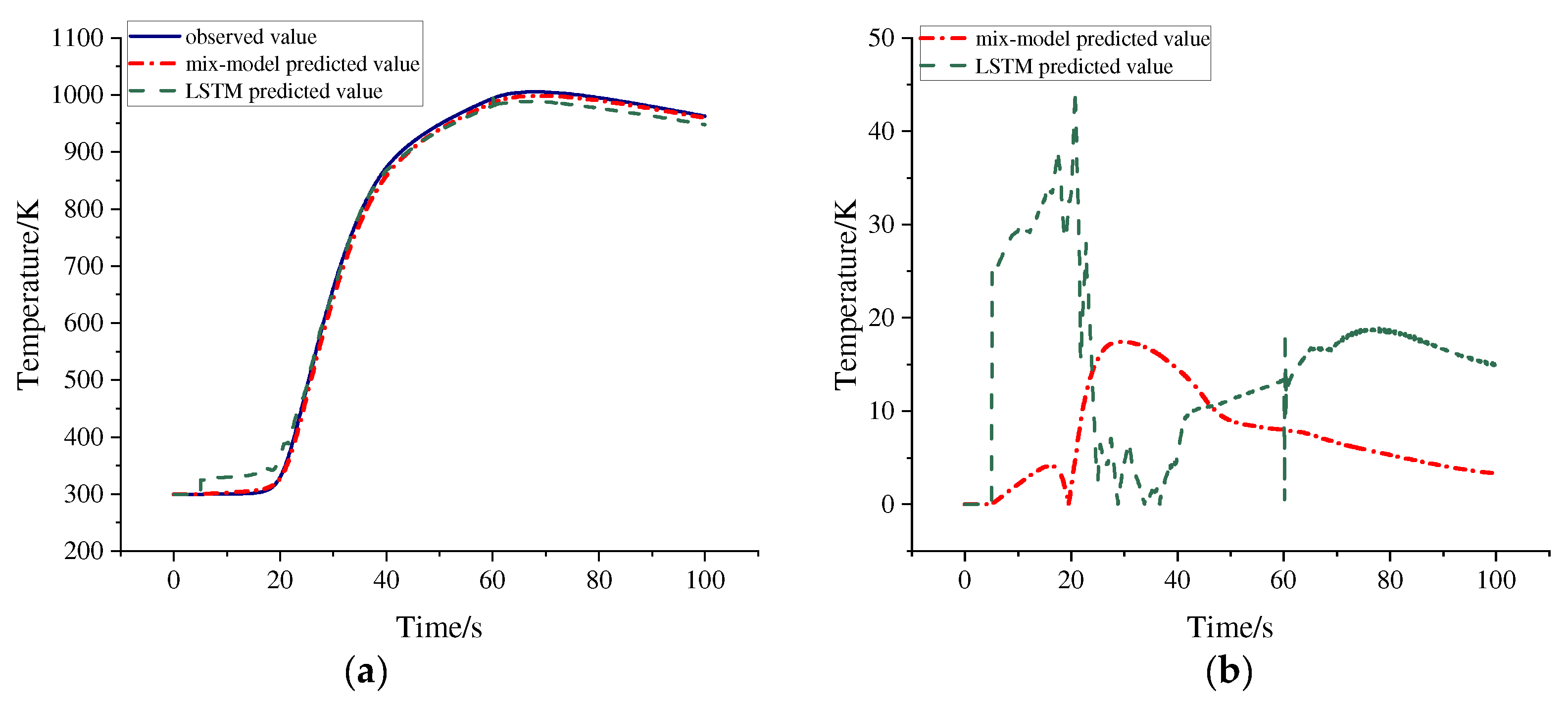
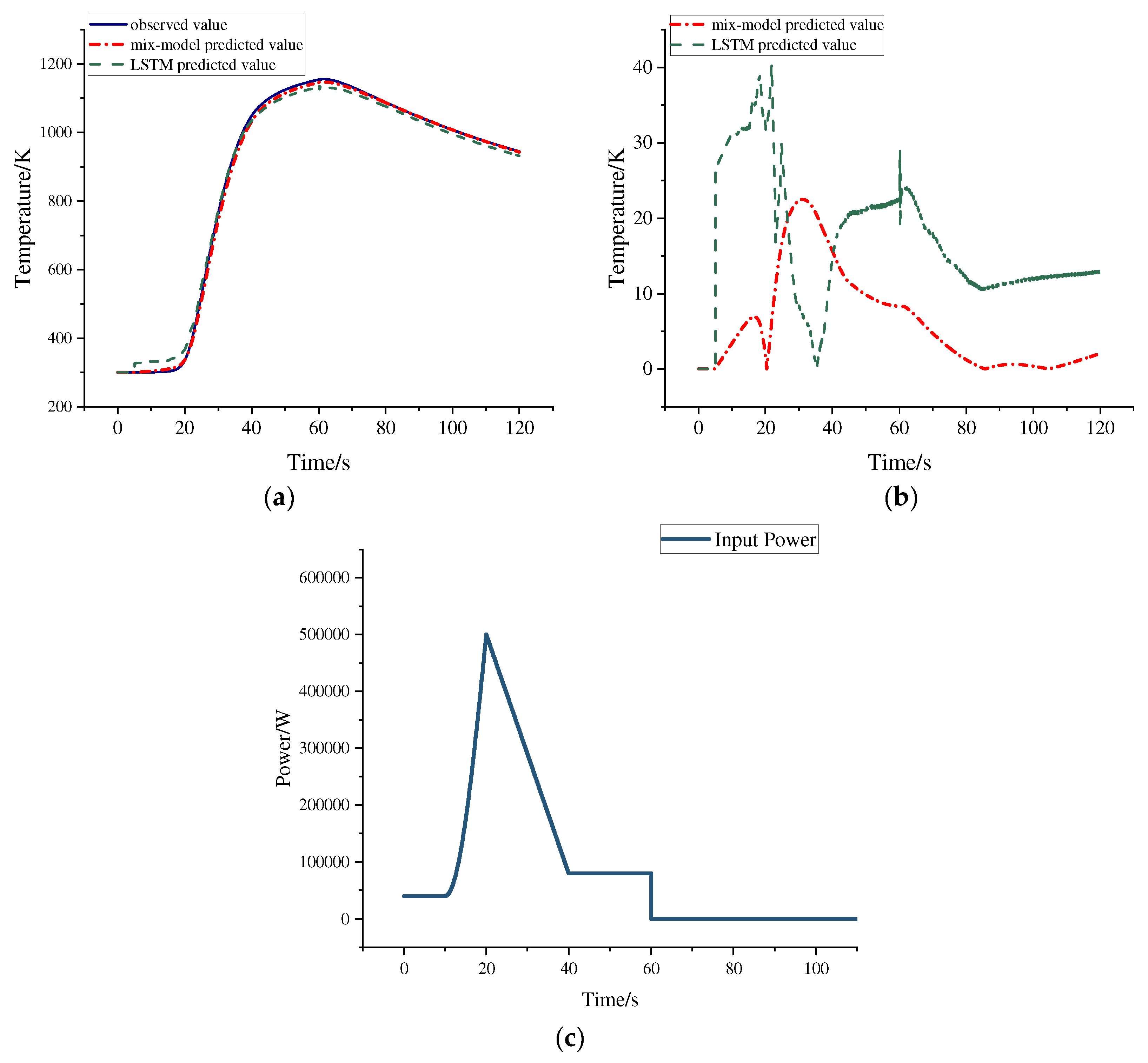
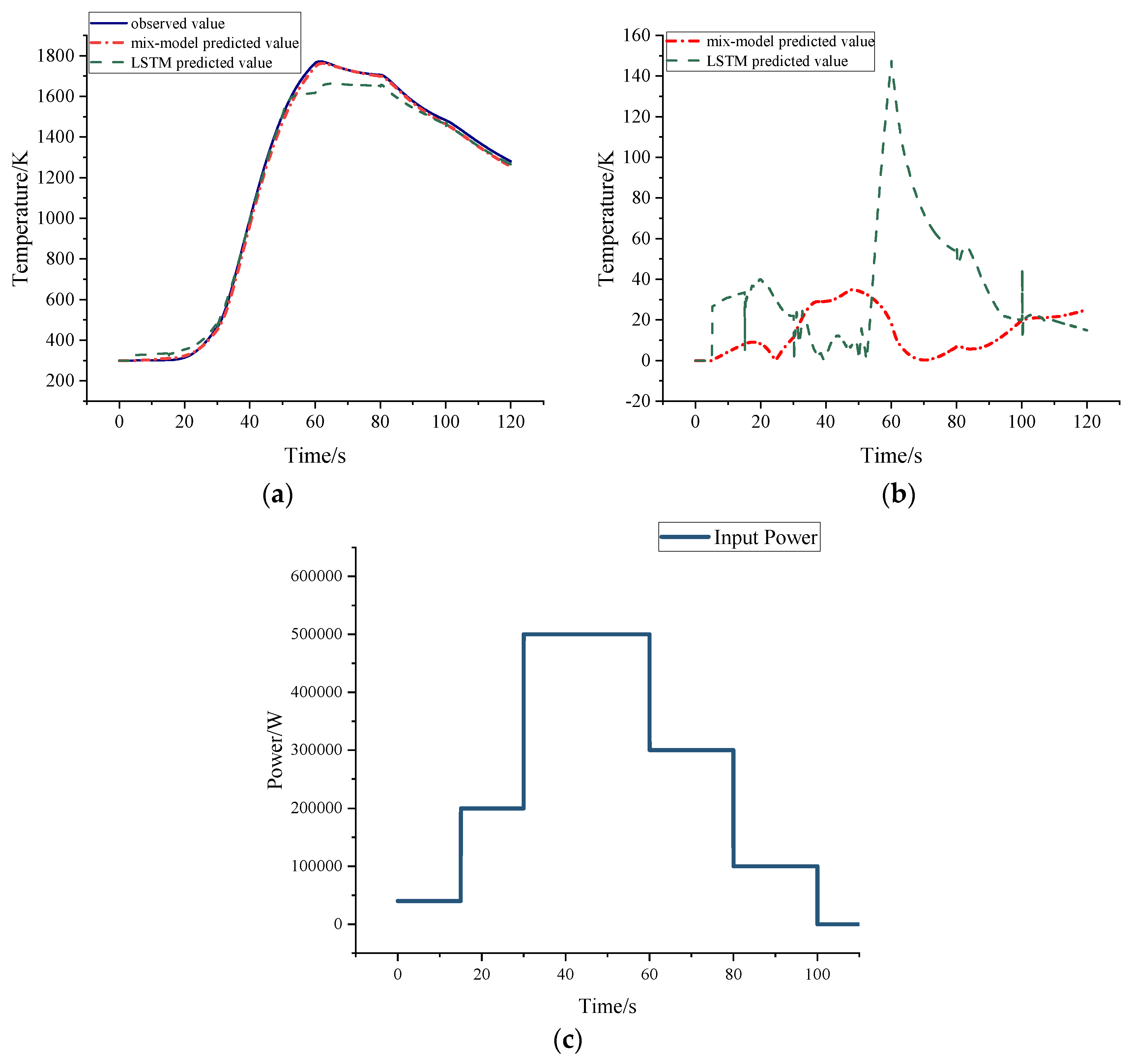
In this paper, we construct the physical model and heat transfer process model for each module of the thermal test system based on its working principles and operational flow. And a temperature prediction method based on the LSTM network with the hybrid model is proposed, and simulation tests are conducted using ANSYS-FLUENT. The simulation data are subsequently used for network training and method validation. The decision coefficients predicted by the hybrid model are 0.9988, 0.9991, and 0.9990 for the three cases of geometric parameter change, material parameter change, and input curve working condition change, respectively. These values exceed the coefficient of determination predicted by the LSTM model, thereby validating the accuracy and robustness of the proposed hybrid model for temperature prediction.

The results of this study illustrate the effectiveness of the hybrid model prediction method that combines the LSTM network with a physical model for predicting test article temperatures in aerospace thermal tests. This approach leverages the strengths of both empirical and physical models, demonstrating versatility and accuracy across different test articles. Ultimately, the method enhances the modeling efficiency and reduces the modeling costs associated with aerospace thermal test systems for various test articles, smoothing the way for the development of more complex models capable of identifying and adapting to diverse test articles. This method can be employed to develop a thermal test forecasting system, which, when integrated with relevant intelligent control algorithms, can adjust control inputs based on predicted thermal test results. This approach not only prevents damage to test articles due to over-control but also enhances the accuracy and reliability of thermal response analysis for aerospace components.

References

1. Zhang, L.S.; Yu, J.J. Thermal Protection Technology for Hypersonic Vehicles; Science Press: Beijing, China, 2021. [Google Scholar]
2. Hargis, C.B. The X-20 (Dyna-Soar) Progress Report; NASA-72-N-71619; NASA: Washington, DC, USA, 1972.
3. Zhang, Y.T.; Li, Y.Y. Causes of the Space Shuttle Columbia crash and analysis of its materials. High Technol. 2005, 23, 34–37. [Google Scholar]
4. Shen, C.; Sun, F.X.; Sia, X.L.; Cao, Z.W.; Yu, M.X.; Wang, Z.F. Aerodynamic Heating Transient Characteristics of Localized Porous Wall-Cavity Structures. J. Astronaut. 2012. [Google Scholar]
5. Cui, Z.; Wang, L. Thermal Characterization of Quartz Lamp Heaters. Strength Environ. 2004, 31, 40–44. [Google Scholar]
6. Zhang, W.; Wang, L.S.; Wang, M.K.; Wang, Q.S.; Ju, Y.T. Research on the Control of the Heating System of Pneumatic Heating Simulation Test. Strength Environ. 2005, 32, 45–52. [Google Scholar]
7. He, Z.; Yang, G.; Zu, J.R.; Li, B. Modeling and Characterization of the Temperature Control System for Hot and Cold Airflow Hybrid Chamber. Hydraul. Pneum. 2023, 47, 26–33. [Google Scholar]
8. Hampson, R.; Dobie, G. Steady State Physical Modeling for Optimizing Capacitive Tactile Sensors Thermal Sensitivity. IEEE Sens. 2023, 23, 26047–26054. [Google Scholar] [CrossRef]
9. LeCun, Y.; Bengio, Y.; Hinton, G. Deep Learning. Nature 2015, 521, 436. [Google Scholar] [CrossRef]
10. Zhang, L.; Zhang, L.; Du, B. Deep Learning for Remote Sensing Data: A Technical Tutorial on the State of the Art. IEEE Geosci. Remote Sens. Mag. 2016, 4, 22–40. [Google Scholar] [CrossRef]
11. Zhu, X.X.; Tuia, D.; Mou, L.; Xia, G.-S.; Zhang, L.; Xu, F.; Fraundorfer, F. Deep Learning in Remote Sensing: A Comprehensive Review and List of Resources. IEEE Geosci. Remote Sens. Mag. 2017, 5, 8–36. [Google Scholar] [CrossRef]
12. Han, Z.Y.; Zhao, J.; Leung, H.; Ma, K.F.; Wang, W. A Review of Deep Learning Models for Time Series Prediction. IEEE Sens. J. 2019, 21, 7833–7848. [Google Scholar] [CrossRef]
13. Li, J.; Wu, G.F.; Zhang, Y.P. Optimizing Flood Predictions by Integrating LSTM and Physical-Based Models with Mixed Historical and Simulated Data. Heliyon 2024, 10, e33669. [Google Scholar] [CrossRef] [PubMed]
14. Kussul, N.; Shelestov, A.; Lavreniuk, M.; Butko, I.; Skakun, S. Deep Learning Approach for Large Scale Land Cover Mapping Based on Remote Sensing Data Fusion. In Proceedings of the 2016 IEEE International Geoscience and Remote Sensing Symposium (IGARSS), Beijing, China, 10–15 July 2016; pp. 198–201. [Google Scholar]
15. Lv, Y.; Duan, Y.; Kang, W.; Li, Z.; Wang, F.-Y. Traffic Flow Prediction with Big Data: A Deep Learning Approach. IEEE Trans. Intell. Transp. Syst. 2015, 16, 865–873. [Google Scholar] [CrossRef]
16. Gensler, A.; Henze, J.; Sick, B. Deep Learning for Solar Power Forecasting—An Approach Using AutoEncoder and LSTM Neural Networks. In Proceedings of the 2016 IEEE International Conference on Systems, Man, and Cybernetics (SMC), Budapest, Hungary, 9–12 October 2016; pp. 2858–2865. [Google Scholar]
17. Fang, J.; Huang, T.; Li, M.; Wang, Y. A Modeling Method for Temperature-Strain Mapping of Bridges Based on Migration Learning and Bi-LSTM Neural Network. Vib. Shock. 2023, 42, 126–134. [Google Scholar]
18. Ding, P.; Zhang, H.; Zhao, X.L. Intelligent Thermal Error Prognostics of Gear Grinding Machine Spindle Based on Model-Data Fusion Approach. IEEE Sens. 2024, 24, 29074–29085. [Google Scholar] [CrossRef]
19. Ni, Q.; Ji, J.C.; Halkon, B.; Feng, K.; Nandi, A.K. Physics-Informed Residual Network (PIRes Net) for Rolling Element Bearing Fault Diagnostics. Mech. Syst. Signal Process. 2023, 200, 110544. [Google Scholar] [CrossRef]
20. Grover, A.; Kapoor, A.; Horvitz, E. A Deep Hybrid Model for Weather Forecasting. In Proceedings of the KDD ‘15: Proceedings of the 21th ACM SIGKDD International Conference on Knowledge Discovery and Data Mining, Sydney, NSW, Australia, 10–13 August 2015; pp. 379–386. [Google Scholar]
21. Yan, M.C.; Yu, Y.; Li, J.L.; Shi, Y.X. Progress in Thermal-Mechanical Coupling Testing and Evaluation Techniques for Hypersonic Vehicle Structures. Flight Guid. Missile 2015, 2, 84–87. [Google Scholar]
22. Shang, L.; Wu, D.; Pu, Y.; Wang, H.; Wang, F.; Gao, Z. Experimental Study on the Thermal Insulation Performance of Lightweight Thermal Protection Materials for Hypersonic Vehicles in an Oxygen Environment at 1700 °C. Spacecr. Environ. Eng. 2016, 42, 7–12. [Google Scholar]
23. Xia, L.S.; Qi, B.; Zhang, X.; Zou, Y. Thermal Environment Analysis of Plate-Type Quartz Lamp Heaters for Thermal Insulation Testing. Infrared Technol. 2016, 38, 617–621. [Google Scholar]
24. Wang, L.S.; Wang, Q.S. Recent Developments in Structural Thermal Testing Technology. Missile Aerosp. Transp. Technol. 2000, 2, 7. [Google Scholar]
25. Qin, Q.Q.; Ren, Q.M.; Wang, Q.; Jiang, J.L.; Cheng, Z. The Impact of Aerodynamic Pressure on the Thermal Insulation Performance of Flexible Thermal Protection Structures. Aerosp. Mater. Technol. 2010, 40, 81–83. [Google Scholar]
26. Wu, D.F.; Pan, B.; Zheng, L.M.; Wang, W.Y.; Mou, M.; Zhu, S.; Li, S. Simulation Methods and Experimental Research on Aerodynamic Thermal Environment for Hypersonic Vehicle Materials and Structures. Spacecr. Environ. Eng. 2012, 29, 250–258. [Google Scholar]
27. Zhao, B.P.; Yan, C.Y.; Meng, X.N.; Liu, P.; Sun, L.; Li, Y.; Cai, J.; Wang, X. Recent Advances in Large Thermal Environment Testing Technology. J. Therm. Environ. Test. 2016, 13, 1–9. [Google Scholar]
28. He, Q.H.; Liu, J.; Tian, Y.K.; Wang, W.; Liu, Y. Research on Control Technology for Structural Thermal Testing of Hypersonic Vehicles in Low-Pressure Environments. Strength Environ. 2019, 46, 9–15. [Google Scholar]
29. Wang, D.C.; Lin, H. Analysis of Key Technologies for Quartz Lamp Radiation-Based Transient Thermal Environment Testing. Equip. Environ. Eng. 2016, 13, 36–40. [Google Scholar]
30. Gers, F.A.; Schmidhuber, J.; Cummins, F. Learning to Forget: Continual Prediction with LSTM; IDSIA-01-99; Istituto Dalle Molle di Studi sull’ Intelligenza Artificiale: Manno, Switzerland, 1999. [Google Scholar]
31. Jaber, F.H.; Shukla, S. Accuracy of hydrodynamic modeling of flood detention reservoirs. J. Hydrol. Eng. 2007, 12, 225–230. [Google Scholar] [CrossRef]
32. Zhang, K. Research on Graphite Heating Elements and Their Heating Control Methods. Master’s Thesis, China Aerospace Science and Technology Corporation, Beijing, China, 2017. [Google Scholar]
Figure 1. Conical thermal test device.
Aerospace 11 00964 g001
Figure 2. Thermal test system workflow.
Aerospace 11 00964 g002
Figure 3. Mechanical model of the thermal test system.
Aerospace 11 00964 g003
Figure 4. Principle of the hybrid model methodology.
Aerospace 11 00964 g004
Figure 5. LSTM network structure.
Aerospace 11 00964 g005
Figure 6. Structure of the LSTM model for the heat transfer process.
Aerospace 11 00964 g006
Figure 7. Mechanism of the sliding window operation.
Aerospace 11 00964 g007
Figure 8. Structured workflow for generalized hybrid model prediction methods.
Aerospace 11 00964 g008
Figure 9. ANSYS-FLUENT platform simulation data: (a) heat flow profile of the heater; (b) heat flow profile of the test article; (c) temperature profile of the heater; (d) temperature profile of the test article; (e) heater input power curve.
Aerospace 11 00964 g009
Figure 10. Temperature prediction results for Model 4 titanium test article impact conditions: (a) temperature prediction curves; (b) prediction vs. observation error curves.
Aerospace 11 00964 g010
Figure 11. Model 4 temperature prediction results for impact conditions of the carbon fiber test article: (a) temperature prediction curves; (b) prediction vs. observation error curves; (c) heater input power curve.
Aerospace 11 00964 g011
Figure 12. Model 4 step condition temperature prediction results for the carbon fiber test article: (a) temperature prediction curves; (b) prediction vs. observation error curves; (c) heater input power curve.
Aerospace 11 00964 g012