Optimal Guidance Law for Critical Safe Miss Distance Evasion

Abstract

In pursuit–evasion scenarios, the pursuer typically possesses a lethal zone. If the evader effectively utilizes perceptual information, they can narrowly escape the lethal zone while minimizing energy consumption, thereby avoiding excessive and unnecessary maneuvers. Based on optimal control theory, we propose a guidance law for achieving critical safe miss distance evasion under bounded control. First, we establish the zero-effort miss (ZEM) state equation for the evader, while approximating disturbances from the pursuer. Next, we formulate an optimal control problem with energy consumption as the objective function and the ZEM at the terminal time as the terminal constraint. Subsequently, we design an iterative algorithm that combines the homotopy method and Newton’s iteration to solve the optimal control problem, applying Pontryagin’s Maximum Principle. The simulation results indicate that the designed iterative method converges effectively; through online updates, the proposed guidance law can successfully achieve critical safe miss distance evasion. Compared to programmatic maneuvering and norm differential game guidance law, this approach not only stabilizes the evader’s evasion capabilities but also significantly reduces energy consumption.

1. Introduction

In certain evasive situations, a larger miss distance is not always preferable. An excessive miss distance may result in unnecessary energy waste and hinder course recovery. For instance, when an unmanned aerial vehicle (UAV) primarily tasked with engaging a target is evading an interceptor, completing the evasion with a large miss distance may result in insufficient energy to engage the subsequent target. Critical safe miss distance evasion refers to evasive action that ensures the miss distance exceeds a critical safe value while minimizing energy consumption. Consequently, critical safe miss distance evasion represents a more efficient maneuvering strategy [1].

Traditional maneuver evasion techniques primarily consist of programmatic maneuvers such as sinusoidal maneuvers [2] and spiral maneuvers [3], which exhibit relatively low levels of proactivity. With the advancements in optimal control theory, methods utilizing detected pursuer information for active evasion have become mainstream. These methods involve the application of Pontryagin’s Maximum Principle and differential game theory to derive analytical solutions for optimal guidance laws [4,5,6]. Recently, scholars have expanded and refined research on optimal maneuver evasion strategies by incorporating high-order complex models, conditions of incomplete information, and multi-agent cooperative evasion strategies. For instance, reference [7] investigated optimal maneuver evasion strategies by establishing a high-order guidance system state-space model for interceptors under proportional guidance control, and utilizing a formula for miss distance series. Reference [8] combined guidance laws derived from complete and incomplete information models using mixed-strategy game theory to propose a new adaptive weighted differential game guidance law. Reference [9] integrated the covariance matrix analysis of Kalman filtering into differential game theory to propose an orientation-driven guidance law. Additionally, references [10,11,12] developed maneuver evasion guidance laws for evaders in active defense scenarios using differential game theory. In the study of the one-evader two-pursuer game problem, the work in reference [13] is based on ideal dynamic characteristics, whereas reference [14] adopted first-order dynamic assumptions and bounded control. Furthermore, with the development of machine learning, intelligent evasion methods have been proposed, such as acquiring evasion guidance law through deep reinforcement learning [15] and employing machine learning to identify saddle-point solutions in nonlinear optimal control problems [16,17].

The aforementioned methods provide robust guidance laws for evasion in various scenarios. However, the objective function, which aims to maximize the miss distance, often results in excessive energy consumption and over-maneuvering issues. To address this, traditional solutions propose treating the control variables as process costs, which are subsequently weighted with terminal costs to form a quadratic differential game [18]. Nevertheless, quadratic differential games yield suboptimal solutions, as they do not consider the boundaries of control variables when solving for co-state variables, and the weighting parameters for the objective function necessitate manual tuning. Consequently, building on previous optimal control theories, several studies have explored optimal guidance laws under critical safe miss distance constraints. Reference [19] derived a solution for the critical safe miss distance evasion problem in a two-dimensional plane under bounded control. However, the miss distance constraint remains a soft constraint weighted within the objective function. Reference [1] employed a similar objective function to investigate three-dimensional critical safe miss distance guidance laws and optimized the selection of the miss distance setting in the objective function using a neural network surrogate model. Reference [20] simplified the evasion maneuver problem to the timing of maneuver selection and utilized LSTM networks to predict the intercept miss distance in real-time during flight, thereby determining the optimal timing for evasion. However, this method does not analyze its optimality.

As discussed above, the current research on critical safe miss distance evasion remains incomplete, particularly regarding the optimality of energy consumption. To address this gap, this study focuses on the maneuvering evasion problem in three-dimensional space, formulating a guidance law for critical safe miss distance evasion grounded in optimal control theory. Initially, the state equation for the zero-effort miss (ZEM) in three-dimensional space is established by treating the pursuer’s maneuvers as disturbances and estimating their values. Subsequently, an optimal control problem is formulated with the control cost defined as the objective function and the ZEM at the terminal time specified as the terminal constraint. The problem is subsequently solved using Pontryagin’s Maximum Principle and iterative algorithms. Finally, the effectiveness of the proposed method is validated through comparative simulations.

This paper presents three substantial and innovative contributions. First, the consideration of bounded control enhances the realism of the modeling process. The introduction of bounded control also complicates the optimal control problem, necessitating an iterative solution approach. Second, it introduces a maneuver estimation method for the pursuer, effectively transforming the game problem into a unilateral optimal control problem, thereby significantly simplifying the derivation of the optimal solution. Third, the miss distance constraint is no longer weighted within the objective function, filling a gap in the research on critical safe miss distance evasion regarding terminal constraints. The terminal constraints are more aligned with the actual requirements of critical miss distance. This research can enrich the evasion strategies and provide valuable insights for optimal maneuvering strategies under other complex model constraints.

2. Optimal Control Problem of Critical Safe Miss Distance Evasion

2.1. Dynamics of Pursuer and Evader

In this paper, both the pursuer and the evader are modeled with constant-speed, three-degree-of-freedom vehicle dynamics. As illustrated in Figure 1, the evader’s initial position is defined as the origin O, and the OX axis is oriented along the evader’s target direction within the horizontal plane. The OY axis is vertical and points upward, and the OZ axis completes the right-handed coordinate system. Thus, we have the following:

$$\left\{\begin{array}{l}{\dot{x}}_i=V_i\cos {\theta }_i\cos {\sigma }_i\\ {\dot{y}}_i=V_i\sin {\theta }_i\\ {\dot{z}}_i=-V_i\cos {\theta }_i\sin {\sigma }_i\\ {\dot{\theta }}_i=\left(a_{yi}-g\cos {\theta }_i\right)/V_i\\ {\dot{\sigma }}_i=-a_{zi}/\left(V_i\cos {\theta }_i\right)\end{array}\right.$$

(1)

where the subscripts $i=E,P$ denote the evader and pursuer, respectively; $\left(x_i,y_i,z_i\right)$ represents the position; $V_i$ is the speed; ${\theta }_i$ is the trajectory inclination angle; ${\sigma }_i$ is the trajectory deflection angle; and $g$ is the gravitational acceleration. $a_{yi}$ and $a_{zi}$ are the normal control accelerations that are perpendicular to the velocity vector, with $a_{yi}$ lying in the plane containing the velocity vector and $a_{zi}$ lying in the horizontal plane. Let $a_i={\left[\begin{array}{cc}{a}_{yi}& a_{zi}\end{array}\right]}^{\mathrm{T}}$, and the upper limit of control is $a_{i,\max }$. Equation (1) is based on the aircraft dynamic model presented in reference [1], with the gravitational acceleration and control acceleration separated to emphasize their independent effects on the dynamics.

Figure 1. Relative motion diagram of the pursuer and evader.

In Figure 1, $q_y$ and $q_z$ are the line-of-sight angles in the pitch and yaw directions of the evader, respectively. In the figure, the directions of $q_y$, $q_z$, ${\theta }_E$, and ${\sigma }_P$ are positive, while the directions of ${\sigma }_E$ and ${\theta }_P$ are negative. In this study, the following assumptions are established:

Assumption 1.

The initial relative motion between the pursuer and evader is characterized by a head-on interception, with the line-of-sight angle exhibiting minimal variation throughout most of the engagement process.

Assumption 2.

There is no control delay for either the pursuer or the evader, and both have ideal dynamic characteristics.

Assumption 3.

The evader is aware of the pursuer’s maximum control input and can obtain real-time information on both parties’ velocities and positions.

The head-on interception refers to the pursuer approaching the evader along the direction opposite to the velocity vector of the evader. This interception method facilitates the stable tracking of the evader by the pursuer and enables the interception of a higher-speed evader. Assumptions 1 and 2 simplify the analytical process of the model, ensuring that it can be effectively solved within the constraints of limited derivations and computational methods. Assumption 3 posits that, in engagement scenarios, both parties’ aircrafts are equipped with radar, a velocity detection system, and other relevant equipment.

2.2. State Equation for Zero-Effort Miss

As shown in Figure 2, the normal control acceleration is projected onto the initial line-of-sight coordinate system ${\mathrm{O}-\mathrm{X}}_{\mathrm{L}}{\mathrm{Y}}_{\mathrm{L}}{\mathrm{Z}}_{\mathrm{L}}$, resulting in $\left[u_{xi}{u}_{yi}{u}_{zi}\right],i=E,P$. Let $r$ denote the distance between the two entities, and $\mathit{r}={\mathit{r}}_E-{\mathit{r}}_P$ represent the distance vector. Let $y_d$ and $z_d$ denote the components of the distance vector along the ${\mathrm{OY}}_{\mathrm{L}}$ and ${\mathrm{OZ}}_{\mathrm{L}}$ axes, respectively. Then, we have the following:

$$\left\{\begin{array}{l}{\ddot{y}}_d=u_{yE}-u_{yP}\\ {\ddot{z}}_d=u_{zE}-u_{zP}\end{array}\right.$$

(2)

Figure 2. Projection of control acceleration in initial line-of-sight coordinate system.

In calculating the time-to-go, it is assumed that the impact of the second derivative of distance on the result is relatively small, and the following typical approach is adopted for the estimation [10]:

$$t_g=-{\displaystyle \frac{r}{\dot{r}}}$$

(3)

In the ${\mathrm{OY}}_{\mathrm{L}}$ direction, with ${\left[\begin{array}{cc}{y}_d& {\dot{y}}_d\end{array}\right]}^{\mathrm{T}}$ as the state variable, the state equation is established as follows:

$$\left[\begin{array}{c}{\dot{y}}_d\\ {\ddot{y}}_d\end{array}\right]=\left[\begin{array}{cc}0& 1\\ 0& 0\end{array}\right]\left[\begin{array}{c}{y}_d\\ {\dot{y}}_d\end{array}\right]+\left[\begin{array}{c}0\\ 1\end{array}\right]u_{yE}-\left[\begin{array}{c}0\\ 1\end{array}\right]u_{yP}$$

(4)

At time $t$, the zero-input state transition matrix is introduced:

$$\Phi \left(t_g,t\right)=\exp \left(\left[\begin{array}{cc}0& 1\\ 0& 0\end{array}\right]\left(t_g-t\right)\right)=\left[\begin{array}{cc}1& t_g-t\\ 0& 1\end{array}\right]$$

(5)

Thus, the zero-effort miss in the ${\mathrm{OY}}_{\mathrm{L}}$ direction at time $t$ is obtained as follows:

$$Z_y\left(t\right)=\left[\begin{array}{cc}1& 0\end{array}\right]\Phi \left(t_g,t\right)\left[\begin{array}{c}{y}_d\\ {\dot{y}}_d\end{array}\right]=y_d+{\dot{y}}_d\left(t_g-t\right)$$

(6)

Similarly, the zero-effort miss in the $O{Z}_L$ direction is as follows:

$$Z_z\left(t\right)=\left[\begin{array}{cc}1& 0\end{array}\right]\Phi \left(t_g,t\right)\left[\begin{array}{c}{z}_d\\ {\dot{z}}_d\end{array}\right]=z_d+{\dot{z}}_d\left(t_g-t\right)$$

(7)

Taking the derivatives of $Z_y$ and $Z_z$, and combining the result with Equation (2), we obtain the following:

$$\left\{\begin{array}{l}{\dot{Z}}_y\left(t\right)={\dot{y}}_d+{\ddot{y}}_d\left(t_g-t\right)-{\dot{y}}_d=\left(t_g-t\right)\left(u_{yE}-u_{yP}\right)\\ {\dot{Z}}_z\left(t\right)={\dot{z}}_d+{\ddot{z}}_d\left(t_g-t\right)-{\dot{z}}_d=\left(t_g-t\right)\left(u_{zE}-u_{zP}\right)\end{array}\right.$$

(8)

According to the transformation relationship between the coordinate systems $\mathrm{O}-\mathrm{XYZ}$ and ${\mathrm{O}-\mathrm{X}}_{\mathrm{L}}{\mathrm{Y}}_{\mathrm{L}}{\mathrm{Z}}_{\mathrm{L}}$, we have the following:

$$\left[\begin{array}{c}{u}_{yi}\\ u_{zi}\end{array}\right]=\left[\begin{array}{ccc}0& 1& 0\\ 0& 0& 1\end{array}\right]M\left(q_y,q_z\right)M^{-1}\left({\theta }_i,{\sigma }_i\right)\left[\begin{array}{c}0\\ a_{yi}\\ a_{zi}\end{array}\right],i=E,P$$

(9)

where the transformation matrix function $\mathit{M}$ is given by the following:

$$\mathit{M}\left(\psi ,\zeta \right)=\left[\begin{array}{ccc}\cos \psi \cos \zeta & \sin \psi & -\cos \psi \sin \zeta \\ -\sin \psi \cos \zeta & \cos \psi & \sin \psi \sin \zeta \\ \sin \zeta & 0& \cos \zeta \end{array}\right]$$

(10)

Substituting the above expression into Equation (8), we obtain the following:

$$\left\{\begin{array}{l}{\dot{Z}}_y\left(t\right)=\left(t_g-t\right)\left({\alpha }_{11}{a}_{yE}+{\alpha }_{12}{a}_{zE}+u_{yP}\right)\\ {\dot{Z}}_z\left(t\right)=\left(t_g-t\right)\left({\alpha }_{21}{a}_{yE}+{\alpha }_{22}{a}_{zE}+u_{zP}\right)\end{array}\right.$$

(11)

where the coefficients of the state equation are as follows:

$$\left\{\begin{array}{l}{\alpha }_{11}=\cos q_y\cos {\theta }_E+\sin q_y\sin {\theta }_E\cos \left(q_z-{\sigma }_E\right)\\ {\alpha }_{12}=\sin q_y\sin \left(q_z-{\sigma }_E\right)\\ {\alpha }_{21}=\sin {\theta }_E\sin \left({\sigma }_E-q_z\right)\\ {\alpha }_{22}=\cos \left(q_z-{\sigma }_E\right)\end{array}\right.$$

(12)

Thus, we have obtained the state equation for the zero-effort miss.

2.3. Objective Function and Constraints

To transform the critical safe miss distance evasion problem into a unilateral optimal control problem, the ZEM caused by the maneuvers of the pursuer and evader is addressed separately. By integrating Equation (11), the miss distance at time $t_g$ is obtained:

$$\left\{\begin{array}{l}{Z}_y\left(t_g\right)=Z_{y,0}+{\displaystyle {\int }_0^{t_g}\left(t_g-t\right)\left({\alpha }_{11}{a}_{yE}+{\alpha }_{12}{a}_{zE}\right)\mathrm{d}t}+{\displaystyle {\int }_0^{t_g}-\left(t_g-t\right)u_{yP}\mathrm{d}t}\\ Z_z\left(t_g\right)=Z_{z,0}+{\displaystyle {\int }_0^{t_g}\left(t_g-t\right)\left({\alpha }_{21}{a}_{yE}+{\alpha }_{22}{a}_{zE}\right)\mathrm{d}t}+{\displaystyle {\int }_0^{t_g}-\left(t_g-t\right)u_{zP}\mathrm{d}t}\end{array}\right.$$

(13)

The integral terms of the pursuer are considered as disturbances and are approximated using the following method. At $t=0$, the pursuer’s strategy is assumed to minimize the absolute value of the initial ZEM by the terminal time. When $0.5a_{P,\max }{t}_g^2\ge \sqrt{Z_{y,0}^2+Z_{z,0}^2}$, if $u_{yp}=2Z_{y,0}/t_g^2$ and $u_{zp}=2Z_{z,0}/t_g^2$, according to Equation (13), it can be ensured that ${\displaystyle {\int }_0^{t_g}-\left(t_g-t\right)u_{yP}\mathrm{d}t}=-Z_{y,0}$ and ${\displaystyle {\int }_0^{t_g}-\left(t_g-t\right)u_{zP}\mathrm{d}t}=-Z_{z,0}$, meaning that the pursuer can successfully eliminate the initial ZEM at the terminal time. When $0.5a_{P,\max }{t}_g^2<\sqrt{Z_{y,0}^2+Z_{z,0}^2}$, the pursuer is unable to fully eliminate the initial ZEM. In this case, the maximum control $a_{P,\max }$ is distributed proportionally between the two directions, i.e., setting $u_{yp}=a_{P,\max }{Z}_{y,0}/\sqrt{Z_{y,0}^2+Z_{z,0}^2}$ and $u_{zp}=a_{P,\max }{Z}_{z,0}/\sqrt{Z_{y,0}^2+Z_{z,0}^2}$. Based on the above approximation method, the disturbance terms are calculated as follows:

$$I_{dy}={\displaystyle {\int }_0^{t_g}-\left(t_g-t\right)u_{yP}\mathrm{d}t}\approx -Z_{y,0}\mathrm{sat}\left({\displaystyle \frac{0.5a_{P,\max }{t}_g^2}{\sqrt{Z_{y,0}^2+Z_{z,0}^2}}}\right)$$

(14)

$$I_{dz}={\displaystyle {\int }_0^{t_g}-\left(t_g-t\right)u_{zP}\mathrm{d}t}\approx -Z_{z,0}\mathrm{sat}\left({\displaystyle \frac{0.5a_{P,\max }{t}_g^2}{\sqrt{Z_{y,0}^2+Z_{z,0}^2}}}\right)$$

(15)

where the saturation function sat is given by the following:

$$\mathrm{sat}\left({\displaystyle \frac{a}{b}}\right)\triangleq \left\{\begin{array}{ll}a/b\hfill & ,\left|a\right|<\left|b\right|\hfill \\ \mathrm{sgn}\left(a/b\right)\hfill & ,\left|a\right|\ge \left|b\right|\hfill \end{array}\right.$$

(16)

The basis for the above approximation is that, at $t=0$, the pursuer’s strategy is assumed to minimize the absolute value of the initial ZEM by the terminal time. This approximation considers, on one hand, the limitations of the pursuer’s control and, on the other hand, the trend of the disturbance. Additionally, the approximation can be updated in real time during the guidance process.

Let the ZEM caused by the evader be treated as the new state variables in the optimal control problem, and the new state equation is as follows:

$$\left\{\begin{array}{l}{\dot{Z}}_{yE}\left(t\right)=\left(t_g-t\right)\left({\alpha }_{11}{a}_{yE}+{\alpha }_{12}{a}_{zE}\right)\\ {\dot{Z}}_{zE}\left(t\right)=\left(t_g-t\right)\left({\alpha }_{21}{a}_{yE}+{\alpha }_{22}{a}_{zE}\right)\end{array}\right.$$

(17)

To minimize energy consumption in control, the objective function is defined as follows:

$$J={\displaystyle {\int }_0^{t_g}\frac{1}{2}\left(a_{yE}^2+a_{zE}^2\right)\mathrm{d}t}$$

(18)

The energy is expressed using the energy concept commonly employed in optimal control theory [12], which is the integral of the square of the control acceleration with respect to time. Therefore, the unit of energy in this paper is ${\mathrm{m}}^2\cdot {\mathrm{s}}^{-3}$.

By decoupling the constraints on the terminal ZEM in two directions, the evader’s requirements for the magnitudes of the terminal ZEM in both directions are established to be no less than $Z_{set}$. Consequently, the constraints are defined as follows:

$$\left\{\begin{array}{l}{Z}_{set}-\left|Z_y\left(t_g\right)\right|\le 0\\ Z_{set}-\left|Z_z\left(t_g\right)\right|\le 0\end{array}\right.$$

(19)

In the aforementioned approximate model, the constraints on $Z_y\left(t_g\right)$ and $Z_z\left(t_g\right)$ utilize absolute values. However, in practical applications, to increase the energy consumption of the pursuer, it is necessary for the signs of $Z_y\left(t_g\right)$ and $Z_z\left(t_g\right)$ to match those of $Z_{y,0}$ and $Z_{z,0}$ at the initial time, respectively. Then, we have the following:

$$\left\{\begin{array}{l}{Z}_{set}-\mathrm{sgn}\left(Z_{y,0}\right)Z_y\left(t_g\right)\le 0\\ Z_{set}-\mathrm{sgn}\left(Z_{z,0}\right)Z_z\left(t_g\right)\le 0\end{array}\right.$$

(20)

It is evident that when the initial zero-effort miss is zero, the sign function should not equal zero. Therefore, the sign function is defined as follows:

$$\mathrm{sgn}\left(a\right)\triangleq \left\{\begin{array}{ll}1\hfill & ,a\ge 0\hfill \\ -1\hfill & ,a<0\hfill \end{array}\right.$$

(21)

Moreover, the control is bounded, with the constraints given by the following:

$${‖{\mathit{a}}_E‖}_2\le a_{E,\max }$$

(22)

The preceding discussion outlines the optimal control problem concerning critical safe miss distance evasion, where the constraint on the miss distance is not incorporated into the objective function but is instead treated as a hard constraint. The distinction between the maneuver for a critical safe miss and the traditional maneuver aimed at maximizing the miss distance is illustrated in Figure 3, where $Z_{\max }$ represents the maximized miss distance and $Z_{safe}$ denotes the critical safe miss distance.

Figure 3. Schematic diagram of critical safe miss distance evasion.

3. Solution Method of the Optimal Guidance Law

3.1. Optimal Guidance Law

The aforementioned optimal control problem is solved using the Pontryagin’s Maximum Principle. The Hamiltonian is as follows:

$$H\left(a_{ty},a_{tz},{\lambda }_1,{\lambda }_2,t\right)={\displaystyle \frac{1}{2}}\left(a_{ty}^2+a_{tz}^2\right)+{\lambda }_1\left(t_g-t\right)\left({\alpha }_{11}{a}_{ty}+{\alpha }_{12}{a}_z\right)+{\lambda }_2\left(t_g-t\right)\left({\alpha }_{21}{a}_{ty}+{\alpha }_{22}{a}_z\right)$$

(23)

where ${\lambda }_1$ and ${\lambda }_2$ are co-state variables. According to the Maximum Principle, the adjoint equations are as follows:

$$\left\{\begin{array}{l}{\dot{\lambda }}_1=-{\displaystyle \frac{\partial H}{\partial Z_y}}=0\\ {\dot{\lambda }}_2=-{\displaystyle \frac{\partial H}{\partial Z_z}}=0\end{array}\right.$$

(24)

$$\left\{\begin{array}{l}{\lambda }_1\left(t_g\right)=-{\gamma }_1\mathrm{sgn}\left(Z_{y,0}\right)\\ {\lambda }_2\left(t_g\right)=-{\gamma }_2\mathrm{sgn}\left(Z_{z,0}\right)\end{array}\right.$$

(25)

where ${\gamma }_1$ and ${\gamma }_2$ are Lagrange multipliers. The transversality condition is as follows:

$$\left\{\begin{array}{l}{\gamma }_1\left[Z_{set}-\mathrm{sgn}\left(Z_{y,0}\right)Z_y\left(t_g\right)\right]+{\gamma }_2\left[Z_{set}-\mathrm{sgn}\left(Z_{z,0}\right)Z_z\left(t_g\right)\right]=0\\ Z_{set}-\mathrm{sgn}\left(Z_{y,0}\right)Z_y\left(t_g\right)\le 0\\ Z_{set}-\mathrm{sgn}\left(Z_{z,0}\right)Z_z\left(t_g\right)\le 0\\ {\gamma }_1\ge 0,{\gamma }_2\ge 0\end{array}\right.$$

(26)

The extremum condition states that for any permissible ${a^{\prime }}_{yE}$ and ${a^{\prime }}_{zE}$, the following is held:

$$H\left(a_{yE},a_{zE},{\lambda }_1,{\lambda }_2,t\right)\le H\left({a^{\prime }}_{yE},{a^{\prime }}_{zE},{\lambda }_1,{\lambda }_2,t\right)$$

(27)

By combining the quadratic form in Equation (23) with the control boundary constraint in Equation (22), the optimal control is derived as follows:

$$a_E=\mathrm{sat}\left({\displaystyle \frac{a_{E,\max }}{\left(t_g-t\right)\sqrt{{\left({\lambda }_1{\alpha }_{11}+{\lambda }_2{\alpha }_{21}\right)}^2+{\left({\lambda }_1{\alpha }_{12}+{\lambda }_2{\alpha }_{22}\right)}^2}}}\right)\left[\begin{array}{c}\left(-{\lambda }_1{\alpha }_{11}-{\lambda }_2{\alpha }_{21}\right)\left(t_g-t\right)\\ \left(-{\lambda }_1{\alpha }_{12}-{\lambda }_2{\alpha }_{22}\right)\left(t_g-t\right)\end{array}\right]$$

(28)

Consequently, once the co-state variables are determined, the optimal control can be obtained, which necessitates jointly solving Equations (23)–(28).

3.2. Method for Solving Co-State Variables

As the co-state variables do not possess an analytical solution, a numerical solution method has been designed, consisting of the following steps.

Step 1: Assume ${\lambda }_1={\lambda }_2=0$ and determine whether Equation (26) is satisfied.

According to Equation (25), ${\gamma }_1={\gamma }_2=0$, and the Hamiltonian is as follows:

$$H={\displaystyle \frac{1}{2}}\left(a_{yE}^2+a_{zE}^2\right)$$

(29)

Furthermore, according to Equation (28), $a_{yE}=a_{zE}=0$; then, the following is obtained:

$$\left\{\begin{array}{l}{Z}_y\left(t_g\right)=Z_{y,0}+I_{dy}\\ Z_z\left(t_g\right)=Z_{z,0}+I_{dz}\end{array}\right.$$

(30)

Given that ${\gamma }_1={\gamma }_2=0$, the assumption holds true only if the following is true:

$$\left\{\begin{array}{l}{Z}_{set}-\mathrm{sgn}\left(Z_{y,0}\right)\left(Z_{y,0}+I_{dy}\right)\le 0\\ Z_{set}-\mathrm{sgn}\left(Z_{z,0}\right)\left(Z_{z,0}+I_{dz}\right)\le 0\end{array}\right.$$

(31)

Then, the co-states are obtained as $\left[\begin{array}{cc}{\lambda }_1& {\lambda }_2\end{array}\right]=\left[\begin{array}{cc}0& 0\end{array}\right]$.

Step 2: If the assumption in Step 1 is not satisfied, we can further assume that ${\lambda }_1=0$, ${\lambda }_2\ne 0$ and determine whether Equation (26) is satisfied.

Based on the assumption, it follows that ${\gamma }_1=0$, ${\gamma }_2\ne 0$. The first task is to determine whether $Z_{set}-\mathrm{sgn}\left(Z_{z,0}\right)\left(Z_{z,0}+I_{dz}\right)<0$ is valid. If this condition is satisfied, then ${\gamma }_2=0$, and the assumption ${\lambda }_2\ne 0$ is not valid. Otherwise, the following equality constraint must be met:

$$Z_{set}-\mathrm{sgn}\left(Z_{z,0}\right)Z_z\left(t_g\right)=0$$

(32)

For convenience in subsequent use, the expression above can be rewritten as follows:

$$Z_z\left(t_g\right)-\mathrm{sgn}\left(Z_{z,0}\right)Z_{set}=0$$

(33)

After solving for ${\lambda }_2$ from Equation (33), substitute ${\lambda }_1=0$ and the solution ${\lambda }_2^{\ast }$ into the inequality:

$$Z_{set}-\mathrm{sgn}\left(Z_{y,0}\right)Z_y\left(t_g\right)\le 0$$

(34)

If inequality (34) is satisfied, then the assumption is validated, resulting in the co-states $[\begin{array}{cc}{\lambda }_1& {\lambda }_2\end{array}]=[\begin{array}{cc}0& {\lambda }_2^{\ast }\end{array}]$.

Step 3: If the assumption in Step 2 is not satisfied, we can further assume that ${\lambda }_2=0$, ${\lambda }_1\ne 0$ and determine whether Equation (26) is satisfied.

Similarly, based on the assumption, it follows that ${\gamma }_1\ne 0$, ${\gamma }_2=0$. The first task is to determine whether $Z_{set}-\mathrm{sgn}\left(Z_{y,0}\right)\left(Z_{y,0}+I_{dz}\right)\le 0$ is valid. If this condition is met, then ${\gamma }_1=0$, and the assumption ${\lambda }_1\ne 0$ is not valid. Otherwise, the following equality constraint must be satisfied:

$$Z_y\left(t_g\right)-\mathrm{sgn}\left(Z_{y,0}\right)Z_{set}=0$$

(35)

After solving for ${\lambda }_1$ from Equation (35), substitute ${\lambda }_2=0$ and the solution ${\lambda }_1^{\ast }$ into the inequality:

$$Z_{set}-\mathrm{sgn}\left(Z_{z,0}\right)Z_z\left(t_g\right)\le 0$$

(36)

If inequality (36) is satisfied, then the assumption is validated, resulting in the co-states $[\begin{array}{cc}{\lambda }_1& {\lambda }_2\end{array}]=[\begin{array}{cc}{\lambda }_1^{\ast }& 0\end{array}]$.

Step 4: If the assumption in Step 3 is not valid, then ${\lambda }_1\ne 0$, ${\lambda }_2\ne 0$. According to Equation (26), the following equality constraint must be satisfied:

$$\left\{\begin{array}{l}{Z}_y\left(t_g\right)-\mathrm{sgn}\left(Z_{y,0}\right)Z_{set}=0\\ Z_z\left(t_g\right)-\mathrm{sgn}\left(Z_{z,0}\right)Z_{set}=0\end{array}\right.$$

(37)

Values of ${\lambda }_1$ and ${\lambda }_2$ can be derived from Equation (37).

The steps outlined above detail the process for solving the co-state variables, as illustrated in Figure 4.

Figure 4. Process for solving co-state variables.

3.3. Iteration Method for Solving Nonlinear Equations

Equations (33), (35), and (37) are all nonlinear equations that necessitate iterative solutions. According to Equation (28), ${‖{\mathit{a}}_E‖}_2$ exhibits two types of variation curves, with $t_x$ in Figure 5 representing the inflection point of the control variable.

Figure 5. Two variation curves of ${‖{\mathit{a}}_E‖}_2$.

When solving Equation (33), the assumptions ${\lambda }_1=0$ and ${\lambda }_2\ne 0$ are made. By combining Equations (13) and (28), the variation of ${‖{\mathit{a}}_E‖}_2$ corresponds to Case 1 when the following is obtained:

$$\left|{\displaystyle \frac{3{\alpha }_{22}\left[\mathrm{sgn}\left(Z_{z,0}\right)Z_{set}-Z_{z,0}-I_{dz}\right]}{t_g^2\left(-{\alpha }_{21}^2-{\alpha }_{22}^2\right)}}\right|\le a_{t,\max }$$

(38)

At this point, ${\lambda }_2$ does not require iterative solving and is expressed as follows:

$${\lambda }_2={\displaystyle \frac{3\left[\mathrm{sgn}\left(Z_{z,0}\right)Z_{set}-Z_{z,0}-I_{dz}\right]}{t_g^3\left(-{\alpha }_{21}^2-{\alpha }_{22}^2\right)}}$$

(39)

For Case 2, the nonlinear equation required for the iteration process in Equation (33) is given by the following:

$$G_2\left({\lambda }_2\right)=Z_{z,0}+I_{dz}+I_h\left({\alpha }_{21},{\lambda }_2\right)+I_h\left({\alpha }_{22},{\lambda }_2\right)-\mathrm{sgn}\left(Z_{z,0}\right)Z_{set}=0$$

(40)

where $I_h\left(\alpha ,\lambda \right)$ is defined as follows:

$$I_h\left(\alpha ,\lambda \right)\triangleq \left\{\begin{array}{ll}-t_g^3{\alpha }^2\lambda /3\hfill & \left|-\lambda \alpha t_g\right|\le a_{E,\max }\hfill \\ \mathrm{sgn}\left(-\lambda \alpha \right)\left[\alpha \left(2t_g{t}_x-t_x^2\right)a_{E,\max }/2\right]-{\left(t_g-t_x\right)}^3{\alpha }^2\lambda /3\hfill & \left|-\lambda \alpha t_g\right|>a_{E,\max }\hfill \end{array}\right.$$

(41)

and $t_x$ can be calculated by the following:

$$t_x=t_g-{\displaystyle \frac{a_{E,\max }}{\left|-\lambda \alpha \right|}}$$

(42)

Similarly, for Equation (35), the variation of ${‖{\mathit{a}}_E‖}_2$ corresponds to Case 1 when the following is obtained:

$$\left|{\displaystyle \frac{3{\alpha }_{11}\left[\mathrm{sgn}\left(Z_{y,0}\right)Z_{set}-Z_{y,0}-I_{dy}\right]}{t_g^2\left(-{\alpha }_{11}^2-{\alpha }_{12}^2\right)}}\right|\le a_{E,\max }$$

(43)

At this point, ${\lambda }_1$ does not require iterative solving, leading to the following:

$${\lambda }_1={\displaystyle \frac{3\left[\mathrm{sgn}\left(Z_{y,0}\right)Z_{set}-Z_{y,0}-I_{dy}\right]}{t_g^3\left(-{\alpha }_{11}^2-{\alpha }_{12}^2\right)}}$$

(44)

For Case 2, the nonlinear equation required for the iteration process in Equation (35) is given by the following:

$$G_1\left({\lambda }_1\right)=Z_{y,0}+I_{dy}+I_h\left({\alpha }_{11},{\lambda }_1\right)+I_h\left({\alpha }_{12},{\lambda }_1\right)-\mathrm{sgn}\left(Z_{y,0}\right)Z_{set}=0$$

(45)

Combining with Equation (28), the system of nonlinear equations required for the iteration process in Equation (37) is given by:

$$\mathit{F}\left({\lambda }_1,{\lambda }_2\right)=\left[\begin{array}{c}{Z}_{y,0}+I_{dy}+I_y\left({\lambda }_1,{\lambda }_2\right)-\mathrm{sgn}\left(Z_{y,0}\right)Z_{set}\\ Z_{z,0}+I_{dz}+I_z\left({\lambda }_1,{\lambda }_2\right)-\mathrm{sgn}\left(Z_{z,0}\right)Z_{set}\end{array}\right]=\left[\begin{array}{c}0\\ 0\end{array}\right]$$

(46)

where

$$\left\{\begin{array}{l}{I}_y\left({\lambda }_1,{\lambda }_2\right)=\left[\left(-{\alpha }_{11}^2-{\alpha }_{12}^2\right){\lambda }_1+\left(-{\alpha }_{11}{\alpha }_{21}-{\alpha }_{12}{\alpha }_{22}\right){\lambda }_2\right]W\left({\lambda }_1,{\lambda }_2\right)\\ I_z\left({\lambda }_1,{\lambda }_2\right)=\left[\left(-{\alpha }_{11}{\alpha }_{21}-{\alpha }_{12}{\alpha }_{22}\right){\lambda }_1+\left(-{\alpha }_{21}^2-{\alpha }_{22}^2\right){\lambda }_2\right]W\left({\lambda }_1,{\lambda }_2\right)\end{array}\right.$$

(47)

For Case 1, when $t_g\sqrt{{\left({\lambda }_1{\alpha }_{11}+{\lambda }_2{\alpha }_{21}\right)}^2+{\left({\lambda }_1{\alpha }_{12}+{\lambda }_2{\alpha }_{22}\right)}^2}\le a_{E,\max }$, the following is obtained:

$$W\left({\lambda }_1,{\lambda }_2\right)=t_g^3/3$$

(48)

In Case 1, Equation (46) is a linear equation in terms of $\mathit{\lambda }={\left[\begin{array}{cc}{\lambda }_1& {\lambda }_2\end{array}\right]}^{\mathrm{T}}$, and it can be solved analytically to yield the following:

$$\lambda ={\left[\begin{array}{ll}{\alpha }_{11}^2+{\alpha }_{12}^2\hfill & {\alpha }_{11}{\alpha }_{21}+{\alpha }_{12}{\alpha }_{22}\hfill \\ {\alpha }_{11}{\alpha }_{21}+{\alpha }_{12}{\alpha }_{22}\hfill & {\alpha }_{21}^2+{\alpha }_{22}^2\hfill \end{array}\right]}^{-1}\left[\begin{array}{c}{Z}_{y,0}+I_{dy}-\mathrm{sgn}\left(Z_{y,0}\right)Z_{set}\\ Z_{z,0}+I_{dz}-\mathrm{sgn}\left(Z_{z,0}\right)Z_{set}\end{array}\right]$$

(49)

For Case 2, when $t_g\sqrt{{\left({\lambda }_1{\alpha }_{11}+{\lambda }_2{\alpha }_{21}\right)}^2+{\left({\lambda }_1{\alpha }_{12}+{\lambda }_2{\alpha }_{22}\right)}^2}\le a_{E,\max }$, the following is obtained:

$$W\left({\lambda }_1,{\lambda }_2\right)={\displaystyle \frac{a_{E,\max }\left(2t_g{t}_x-t_x^2\right)}{2\sqrt{{\left({\lambda }_1{\alpha }_{11}+{\lambda }_2{\alpha }_{21}\right)}^2+{\left({\lambda }_1{\alpha }_{12}+{\lambda }_2{\alpha }_{22}\right)}^2}}}+{\displaystyle \frac{{\left(t_g-t_x\right)}^3}{3}}$$

(50)

where

$$t_x=t_g-{\displaystyle \frac{a_{E,\max }}{\sqrt{{\left({\lambda }_1{\alpha }_{11}+{\lambda }_2{\alpha }_{21}\right)}^2+{\left({\lambda }_1{\alpha }_{12}+{\lambda }_2{\alpha }_{22}\right)}^2}}}$$

(51)

Equations (40) and (45) each possess a single independent variable and are relatively straightforward in form, facilitating the identification of appropriate initial values. Consequently, the Newton iteration method is employed as follows:

$${\lambda }_i^{\left(k+1\right)}={\lambda }_i^{\left(k\right)}-{\displaystyle \frac{G_i\left({\lambda }_i^{\left(k\right)}\right)}{{\dot{G}}_i\left({\lambda }_i^{\left(k\right)}\right)}},k=0,1,\mathrm{\dots },N_n-1;i=1,2$$

(52)

where $N_n$ denotes the upper limit of the Newton iteration. Let the error tolerance be $\epsilon$, and the convergence criterion for iteration process is as follows:

$$\left|{\lambda }_i^{\left(k+1\right)}-{\lambda }_i^{\left(k\right)}\right|\le \epsilon ,i=1,2$$

(53)

To ensure a suitable initial value for the Newton iteration, we assume that $q_z$ and ${\sigma }_E$ differ only slightly. Consequently, ${\alpha }_{12}$ and ${\alpha }_{21}$ are small quantities that can be disregarded, enabling an analytical approximation of $\mathit{\lambda }$:

$${\lambda }_1^{\left(0\right)}=-\mathrm{sgn}\left(Z_{y,0}\right){\left[{\displaystyle \frac{a_{t,\max }^3\mathrm{sgn}\left(Z_{y,0}\right)}{6{\alpha }_{11}\left(Z_{y,0}+I_{dy}+\mathrm{sgn}\left(Z_{y,0}\right)\left({\alpha }_{11}{a}_{t,\max }{t}_g^2/2-Z_{set}\right)\right)}}\right]}^{{\displaystyle \frac{1}{2}}}$$

(54)

$${\lambda }_2^{\left(0\right)}=-\mathrm{sgn}\left(Z_{z,0}\right){\left[{\displaystyle \frac{a_{t,\max }^3\mathrm{sgn}\left(Z_{z,0}\right)}{6{\alpha }_{22}\left(Z_{z,0}+I_{dz}+\mathrm{sgn}\left(Z_{z,0}\right)\left({\alpha }_{22}{a}_{t,\max }{t}_g^2/2-Z_{set}\right)\right)}}\right]}^{{\displaystyle \frac{1}{2}}}$$

(55)

${\lambda }^{\left(0\right)}={\left[{\lambda }_1^{\left(0\right)}{\lambda }_2^{\left(0\right)}\right]}^{\mathrm{T}}$ represent the initial value for the iteration of Equation (52).

To solve Equation (46), a preliminary value is initially calculated based on Equation (49). If the preliminary value satisfies the inequality for Case 1, then $\mathit{\lambda }={\mathit{\lambda }}^{\left(0\right)}$. If the preliminary value does not satisfy Case 1, the iteration solution is required. Due to the coupling between ${\lambda }_1$ and ${\lambda }_2$, the nonlinear equations become more complex, necessitating the adoption of the Newton–homotopy iteration method [21] for the solution:

$$\left\{\begin{array}{l}{\mathit{\lambda }}^{\left(k+1\right)}={\mathit{\lambda }}^{\left(k\right)}-{\left[\nabla \mathit{F}\left({\mathit{\lambda }}^{\left(k\right)}\right)\right]}^{-1}\left[\mathit{F}\left({\mathit{\lambda }}^{\left(k\right)}\right)+\left({\displaystyle \frac{k}{N_h}}-1\right)\mathit{F}\left({\mathit{\lambda }}^{\left(0\right)}\right)\right],k=0,1,\mathrm{\dots },N_h-1\\ {\mathit{\lambda }}^{\left(k+1\right)}={\mathit{\lambda }}^{\left(k\right)}-{\left[\nabla \mathit{F}\left({\mathit{\lambda }}^{\left(k\right)}\right)\right]}^{-1}\mathit{F}\left({\mathit{\lambda }}^{\left(k\right)}\right),k=N_h,N_h+1,\mathrm{\dots },N_h+N_n-1\end{array}\right.$$

(56)

where $N_h$ is the number of homotopy iterations and $N_n$ is the upper limit for the Newton iteration. The homotopy iteration method demonstrates strong adaptability to initial values, so the purpose of $N_h$ iterations is to obtain a suitable initial value for the subsequent Newton iteration. The computed ${\mathit{\lambda }}^{\left(0\right)}$ serves as the initial value for homotopy iteration, and the convergence criterion for Newton iteration is given by the following:

$${‖{\mathit{\lambda }}^{\left(k+1\right)}-{\mathit{\lambda }}^{\left(k\right)}‖}_2\le \epsilon$$

(57)

In summary, once the solution for $\mathit{\lambda }$ is complete, the optimal evasion guidance law can be derived from Equation (28).

4. Simulation and Analysis

4.1. Simulation Setup

Continuous updates to the guidance law during flight are essential due to the simplifications and assumptions inherent in the ZEM model. Given that the simulation time step is frequently shorter than the duration required for an iterative solution, the evader continues to employ the previous guidance law until the updates are finalized. Furthermore, as the distance diminishes, the angle between the evader’s velocity vector and the line-of-sight increases, leading to a heightened linearization error. Consequently, it is mandated that updates to the guidance law and control commands cease when the distance falls below $r_C$. When $r_C$ is too large, it may cause the guidance law to stop updating prematurely. Conversely, if $r_C$ is too small, significant linearization errors may lead to an inaccurate guidance law. According to simulation results, a value of $r_C=500\mathrm{m}$ provides stable guidance and control performance for the evader.

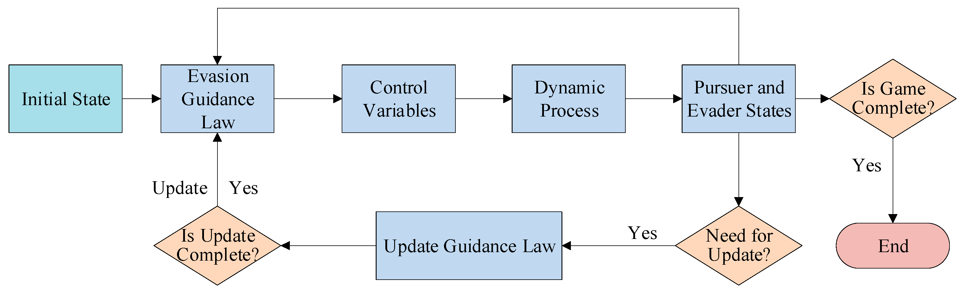
The iteration initial values for the first computation of the guidance law are derived from Section 3.3, whereas the initial values for each subsequent update adopt the calculated result of the preceding update. A concise overview of the simulation process is illustrated in Figure 6, and the general parameters are detailed in Table 1. As indicated in Section 2.3, the critical safe miss distance synthesized in two directions is denoted as $Z_{safe}=\sqrt{2}{Z}_{set}$. The computer hardware configuration comprises an Intel Core i7-13620H processor operating at 4.90 GHz. All results in this study are based on computational simulations and do not include experimental data.

Figure 6. Simulation flow chart.

Table 1. General parameters used in simulation.

Time Step	${\mathit{Z}}_{\mathit{s}\mathit{e}\mathit{t}}$	${\mathit{N}}_{\mathit{n}}$	${\mathit{N}}_{\mathit{h}}$	$\mathit{\epsilon }$	${\mathit{V}}_{\mathit{E}}$	${\mathit{V}}_{\mathit{P}}$	${\mathit{a}}_{\mathit{E},\mathbf{max}}$	${\mathit{a}}_{\mathit{P},\mathbf{max}}$
0.001 s	50 m	50	100	0.001	2 km/s	2 km/s	10 g	12 g

In the simulation, the pursuer’s guidance law employs proportional navigation with bounded control:

$$\left[\begin{array}{c}{a}_{yP}\\ a_{zP}\end{array}\right]=\left[\begin{array}{c}{k}_P{V}_P{\dot{q}}_y\\ k_P{V}_P{\dot{q}}_z\end{array}\right]\mathrm{sat}\left({\displaystyle \frac{a_{P,\max }}{k_P{V}_P\sqrt{{\dot{q}}_y^2+{\dot{q}}_z^2}}}\right)$$

(58)

where $k_P$ is the effective navigation ratio.

4.2. Simulation of Critical Safe Miss Distance Evasion

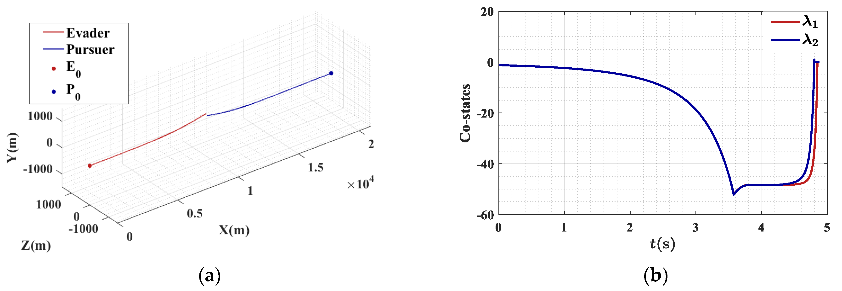
First, simulations were conducted under two typical operating conditions, shown in Table 2, with the effective navigation ratio of the pursuer set to 3. The simulation results are illustrated in Figure 7, Figure 8, Figure 9 and Figure 10. In Figure 7 and Figure 9, points ${\mathrm{E}}_0$ and ${\mathrm{P}}_0$ denote the initial positions of the evader and the pursuer, respectively. The miss distances for two conditions were 70.68 m and 71.37 m, with errors of −0.04% and 0.93% relative to the critical value, respectively. The energy consumption of the evader under two conditions is $4.787\times {10}^3{\mathrm{m}}^2\cdot {\mathrm{s}}^{-3}$ and $8.467\times {10}^2{\mathrm{m}}^2\cdot {\mathrm{s}}^{-3}$, respectively.

Table 2. Initial states under typical conditions.

	Condition 1	Condition 2
$\left[x_E\left(\mathrm{m}\right)y_E\left(\mathrm{m}\right)z_E\left(\mathrm{m}\right){\theta }_E\left(\mathrm{rad}\right){\sigma }_E(\mathrm{rad})\right]$	$\left[00000\right]$	$\left[00000\right]$
$\left[x_P\left(\mathrm{m}\right)y_P\left(\mathrm{m}\right)z_P\left(\mathrm{m}\right){\theta }_P\left(\mathrm{rad}\right){\sigma }_P(\mathrm{rad})\right]$	$\left[20000000\pi \right]$	$\left[2000010001000-0.04993.0916\right]$

Figure 7. Trajectory and co-state variables in Condition 1. (a) The trajectory; (b) the co-state variables.

Figure 8. Evasion and pursuit control commands in Condition 1. (a) a_y; (b) a_z.

Figure 9. Trajectory and co-state variables in Condition 2. (a) The trajectory; (b) the co-state variables.

Figure 10. Evasion and pursuit control commands in Condition 2. (a) a_y; (b) a_z.

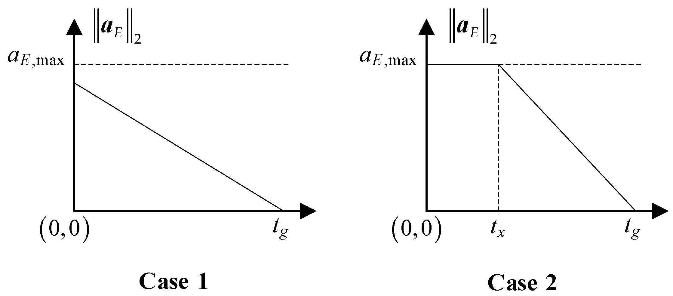
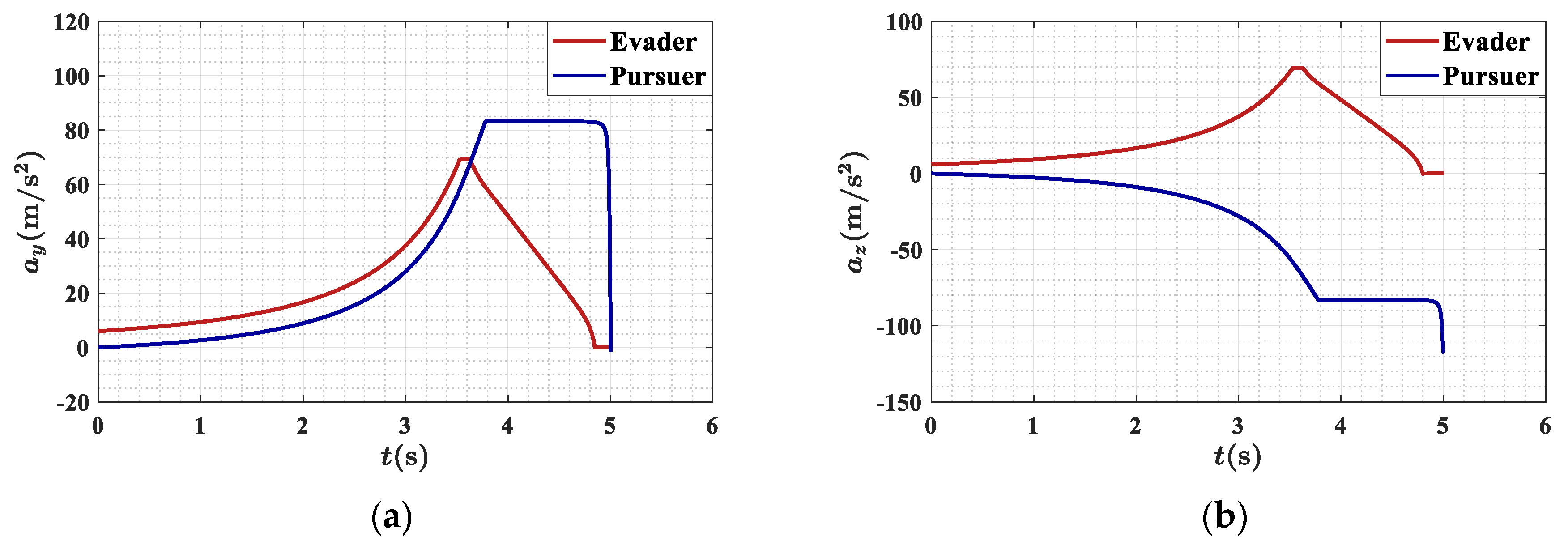
Under both conditions, the miss distances are near the critical safe value, with Condition 2 demonstrating a greater miss distance and reduced energy consumption. This phenomenon is attributed to the initial ZEM of zero in Condition 1, while Condition 2 features a significant initial ZEM of 70.80 m. The absolute values of the evasion control for both conditions display a trend of initially increasing and subsequently decreasing. In Condition 1, when the pursuer’s maximum control commands are insufficient to reduce the ZEM to the critical safe value, the evasion control command becomes zero. In Condition 2, as the time-to-go decreases, the co-state variable in the pitch direction does not converge to zero, leading to a non-zero evasion control command. When the distance between the two parties is below the established threshold of 500 m, the control command remains constant. The average duration for the guidance law updates in two conditions is $3.68\times {10}^{-5}\mathrm{s}$, with a maximum duration of 0.0096 s, which satisfies the requirement for rapid updates.

Monte Carlo simulations were conducted. The initial states were generated uniformly at random within the range specified in Table 3. The random variables for the initial states include the relative positions of two parties and the direction of the evader’s velocity. The evader’s initial position was always located at the origin of the coordinate system, while the direction of pursuer’s initial velocity was oriented toward the evader, aligning with the initial line of sight. To evaluate the adaptability of the guidance law to different effective navigation ratios of pursuer, simulations were conducted 500 times for $k_p=3$ and $k_p=4$, respectively. The simulation trajectories and statistical results are presented in Figure 11. Due to the influence of gravity, the average positions at the interception moment for both parties are significantly lower than the origin. The statistics on the miss distance indicate that the average miss distances for $k_p=3$ and $k_p=4$ are 136.51 m and 116.37 m, respectively, with 12.4% and 32.0% of them falling below the critical value. The minimum miss distances are 70.45 m and 70.37 m, with relative errors to the critical value of −0.37% and −0.48%, respectively. The average energy consumption for the evader is 9.847 × 10² m²·s⁻³ and 2244 × 10³ m²·s⁻³, while for the pursuer, it is $2.435\times {10}^4{\mathrm{m}}^2\cdot {\mathrm{s}}^{-3}$ and $2.627\times {10}^4{\mathrm{m}}^2\cdot {\mathrm{s}}^{-3}$, respectively. In 1000 simulations, the average update time for the guidance law is 1.17 × 10⁻⁵ s, with a maximum update time of 0.0088 s, which meets the requirements for rapid updates.

Table 3. Range of initial states distributions in Monte Carlo simulations.

	θE(rad)	σE(rad)	xP(km)	yP(km)	zP(km)
Range	[−0.1,0.1]	[−0.1,0.1]	[18,22]	[−2,2]	[−2,2]

Figure 11. Trajectories and statistical results of guidance law with critical safe miss distance. (a) The trajectories; (b) the statistical results.

It can be observed that under random initial states, the average miss distance is greater when $k_p=3$ compared to $k_p=4$. The average energy consumption for the evader is higher at $k_p=4$; however, the energy consumption for the pursuer is also greater. When $k_p=3$, Case 1 of ${‖{\mathit{a}}_E‖}_2$ occurs more frequently, leading to more instances in which no iteration is required, resulting in a shorter average update time. Due to simplifications in the optimal control model, the proportion of miss distances below the critical safe value is relatively high. Nevertheless, for both effective navigation ratios, the relative errors of the minimum miss distances compared to the critical safe value are less than 1%, indicating that the guidance law for critical safe miss distance evasion is effective.

4.3. Comparison with Other Methods

To illustrate the effectiveness of the guidance law for critical safe miss distance evasion in reducing energy consumption, comparisons were made with the sinusoidal maneuver, spiral maneuver, and norm differential game maneuver [22]. The sinusoidal and differential game maneuvers are applied in the yaw plane, with the control commands for the three methods detailed in Table 4. Considering that some of the miss distances in Section 4.2 fall below the critical value while the relative error does not exceed 1%, this section modifies the original $Z_{set}=50\mathrm{m}$ in the guidance law to ${Z^{\prime }}_{set}=1.01\times Z_{set}$. Initial states were uniformly and randomly generated within the range specified in Table 3, and 500 simulations were conducted for each of the four methods with $k_p=3$.

Table 4. Control commands for three methods.

Control Variable	Sinusoidal Maneuver	Spiral Maneuver	Norm Differential Game
$a_{yE}$	0	$a_{E,\max }\cos \left(\pi t/4\right)$	0
$a_{zE}$	$a_{E,\max }\sin \left(\pi t/4\right)$	$a_{E,\max }\sin \left(\pi t/4\right)$	$a_{E,\max }\mathrm{sgn}\left(Z_z\left(t\right)\right)$

$a_{yE}$$a_{E,\max }\cos \left(\pi t/4\right)$$a_{zE}$$a_{E,\max }\sin \left(\pi t/4\right)$$a_{E,\max }\sin \left(\pi t/4\right)$$a_{E,\max }\mathrm{sgn}\left(Z_z\left(t\right)\right)$ The simulation results are presented in Table 5 and Figure 12. In Figure 12, the results of the critical safe miss distance maneuver exhibit a significant difference compared to other maneuvering methods. The primary reason for this difference is that the proposed guidance law has an objective function specifically aimed at achieving the critical safe miss distance. In contrast, the programmatic oscillatory maneuvers lack the objective functions, while the norm differential game maneuver is designed to maximize the miss distance. Table 5 provides the statistics of the miss distances and energy consumption, including the mean value, relative standard deviation (RSD), and other relevant statistical metrics. In the context of anti-interception operations, evasion is deemed unsuccessful when the miss distance is less than the critical safe miss distance. In the results of the critical safe miss distance evasion, occurrences of miss distance below the critical value are no longer observed, indicating that the 1% adjustment to $Z_{set}$ is effective. Comparatively, among the four evaluated methods, the critical safe miss distance evasion exhibits the smallest average miss distance. Moreover, the critical safe miss distance evasion has no instances of failure, which is comparable to the differential game maneuver. The energy consumption of the critical safe miss distance evasion is also lower and significantly less than that of the other methods. Although the average miss distances for the sinusoidal and spiral maneuvers are larger, they exhibit relatively high RSDs and greater proportions of failure. This indicates that the miss distances for the programmatic maneuvers are more dependent on initial state values, exhibiting lower proactivity. When flight times are similar, the energy consumption of sinusoidal and spiral maneuvers shows a small variation after fixing the frequency and phase, resulting in lower RSDs in energy consumption. Since the control magnitude of the differential game maneuver is set at $a_{E,\max }$, the differences in flight times are also minimal, leading to a lower RSD for energy consumption.

Table 5. Statistics of miss distance and energy consumption for different methods.

Maneuvering Method	Average Miss (m)	Minimum Miss (m)	RSD of Miss	Failure Proportion	Average Energy Consumption (m2 s−3)	RSD of Energy Consumption
Critical safe miss maneuver	129.70	71.14	82.2%	0	$9.368\times {10}^2$	108.2%
Sinusoidal maneuver	295.52	0.36	90.8%	22.8%	$1.081\times {10}^4$	7.3%
Spiral maneuver	316.76	4.63	85.2%	15.2%	$2.419\times {10}^4$	5.8%
Norm differential	870.74	383.02	35.3%	0	$2.443\times {10}^4$	5.9%

Figure 12. Statistics of miss distances and energy consumption for different methods. (a) The miss distances; (b) the energy consumption.

In summary, the proposed guidance law exhibits a greater probability of successful evasion compared to programmatic oscillatory maneuvers while incurring lower energy costs. Furthermore, in comparison to the norm differential game maneuver, it additionally achieves a reduction in energy consumption and effectively satisfies the requirements for critical safe miss distance evasion.

4.4. Evaluation of the Adaptability to Unpowered Aerial Vehicle

To reduce the mathematical and computational complexity, the proposed guidance law is formulated for the constant-speed vehicle. However, when the engagement time is short and the vehicle’s speed variation is relatively small, the guidance law could be adapted for the unpowered aerial vehicle. The aerodynamic characteristics and mass data for the CAV-H model are provided in reference [23]. In the subsequent simulation, we consider a scenario in which both the pursuer and evader are CAV-H models, aiming to evaluate the adaptability of the guidance law to the more complex model. The specific procedure for applying the guidance law under the CAV-H model is outlined as follows:

Step 1: Determine the maximum control $a_{E,\max }$ and $a_{P,\max }$ based on the current speeds, maximum attack angles, and aerodynamic characteristics of the evader and pursuer.

Step 2: If the guidance law needs to be updated, substitute the current speeds of the evader and pursuer into $V_E$ and $V_P$, respectively, and compute the required acceleration command for the evader.

Step 3: Based on the aerodynamic characteristics of CAV-H, calculate the attack angle ${\alpha }_E$ and the bank angle ${\nu }_E$ from the acceleration command. Substitute the attack angle and bank angle into the CAV-H dynamic model and perform the simulation through numerical integration.

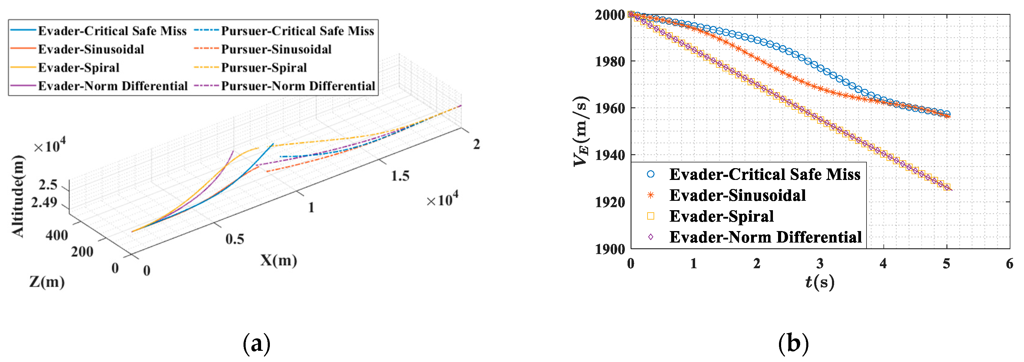
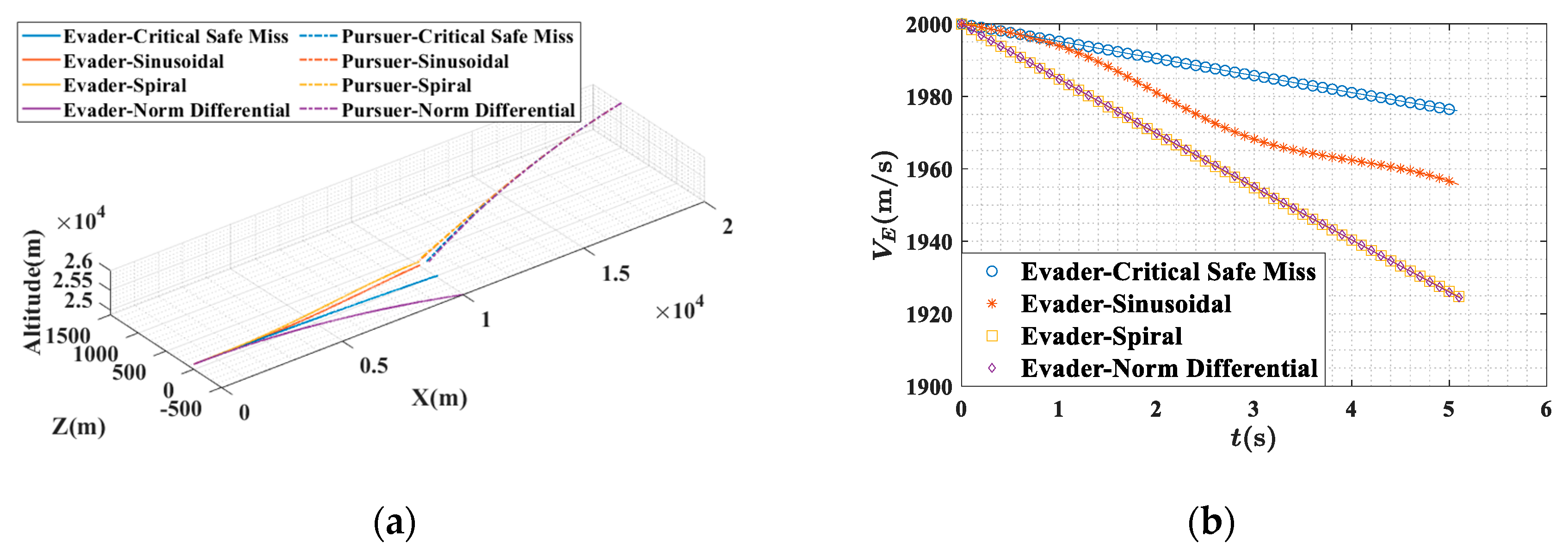
The effective navigation ratio of the pursuer is set to 4, and the initial altitude of the evader is set to 25 km. Under Condition 1 and Condition 2 provided in Table 2, the four guidance laws in Section 4.3 are applied in the simulations. The resulting flight trajectories and speed curves are shown in Figure 13 and Figure 14, while the miss distances and the evader’s terminal speeds are presented in Table 6. For the unpowered vehicle, a larger acceleration in the objective function leads to a larger attack angle, which results in greater speed loss. Therefore, in this section, energy consumption is represented by the evader’s speed loss, defined as the difference between the initial and the terminal speeds. Under both conditions, the miss distance of the critical safe miss distance maneuver exceeds the critical value. The speed curves for the spiral maneuver and the differential game maneuver are similar, as both use maximum overload, resulting in a comparable aerodynamic drag. In Condition 1, the speed loss of the critical safe miss distance maneuver is only slightly lower than that of the sinusoidal maneuver. However, the miss distance of the sinusoidal maneuver is smaller than $Z_{safe}$, whereas the critical safe miss distance maneuver ensures safe evasion. In Condition 2, all the guidance laws achieve safe evasion, with the critical safe miss distance maneuver resulting in the smallest speed loss.

Figure 13. Simulation results of the CAV-H model under Condition 1. (a) The trajectories; (b) the speed curves.

Figure 14. Simulation results of the CAV-H model under Condition 2. (a) The trajectories; (b) the speed curves.

Table 6. Simulation results based on the CAV-H model.

Maneuvering Method	Miss in Condition 1 (m)	Miss in Condition 2 (m)	Speed Loss in Condition 1 (m/s)	Speed Loss in Condition 2 (m/s)
Critical safe miss maneuver	71.23	268.99	42.91	23.97
Sinusoidal maneuver	60.02	123.97	43.98	44.31
Spiral maneuver	72.85	72.45	74.96	75.32
Norm differential	178.24	675.29	75.27	75.77

The results indicate that the critical safe miss distance maneuver can be effectively applied to the CAV-H model. In comparison with the programmatic maneuver and the differential game maneuver, the critical safe miss distance guidance law achieves a safe evasion with smaller speed losses in head-on intercepts.

5. Conclusions

This paper addresses the pursuit–evasion problem for constant-speed vehicles in three-dimensional space and proposes a guidance law for critical safe miss distance evasion. Simulation results validate the effectiveness of the guidance law. The main conclusions are as follows:

Through the state equation of the ZEM and the approximation of the disturbances experienced by the pursuer, an optimal control problem for critical safe miss distance evasion was established. Using the Maximum Principle, the optimal guidance law under bounded control and terminal constraints was derived. Furthermore, an iterative method was designed for solving co-state variables with the homotopy method and Newton iteration.

The simulation results demonstrate that, within a certain range of initial conditions, the proposed iterative method meets real-time requirements. Under head-on intercept conditions, the guidance law effectively achieves critical safe miss distance evasion and adapts to different effective navigation ratios of the pursuer. Compared to other methods, the critical safe miss distance evasion results in a lower probability of the miss distance being below the critical value and incurs a smaller energy cost. In head-on intercept scenarios, the proposed guidance law is applicable to unpowered vehicle models.

Future research will focus on comparing various guidance methods across a broader range of engagement configurations, such as non-head-on intercepts, and improving the feasibility of the proposed guidance law in practical engineering applications.