Comparative Analysis of Deep Reinforcement Learning Algorithms for Hover-to-Cruise Transition Maneuvers of a Tilt-Rotor Unmanned Aerial Vehicle

Abstract

Work on trajectory optimization is evolving rapidly due to the introduction of Artificial-Intelligence (AI)-based algorithms. Small UAVs are expected to execute versatile maneuvers in unknown environments. Prior studies on these UAVs have focused on conventional controller design, modeling, and performance, which have posed various challenges. However, a less explored area is the usage of reinforcement-learning algorithms for performing agile maneuvers like transition from hover to cruise. This paper introduces a unified framework for the development and optimization of a tilt-rotor tricopter UAV capable of performing Vertical Takeoff and Landing (VTOL) and efficient hover-to-cruise transitions. The UAV is equipped with a reinforcement-learning-based control system, specifically utilizing algorithms such as Deep Deterministic Policy Gradient (DDPG), Trust Region Policy Optimization (TRPO), and Proximal Policy Optimization (PPO). Through extensive simulations, the study identifies PPO as the most robust algorithm, achieving superior performance in terms of stability and convergence compared with DDPG and TRPO. The findings demonstrate the efficacy of DRL in leveraging the unique dynamics of tilt-rotor UAVs and show a significant improvement in maneuvering precision and control adaptability. This study demonstrates the potential of reinforcement-learning algorithms in advancing autonomous UAV operations by bridging the gap between dynamic modeling and intelligent control strategies, underscoring the practical benefits of DRL in aerial robotics.

1. Introduction

Due to the emergence of Artificial Intelligence (AI), research on the trajectory optimization of small UAVs is evolving. Such UAVs are expected to be capable of flying in unknown environments. The maneuverability requirement demands efficient path planning, waypoint navigation, autonomous control, and movement. This leads to the planning and development of versatile small Unmanned Aerial Vehicles (UAVs). Once limited to the military, UAVs are now widely used in industrial and commercial sectors. Unmanned aerial vehicles, which vary in shape and size, are a major constituent of Unmanned Aerial Systems (UASs). They range from micro-scale UAVs to larger, high-altitude aircraft. This research focuses on small UAVs that can perform agile maneuvers, from hovering to cruising.

Managing agile and autonomous UAVs is more challenging than controlling other man-made flying vehicles. The flight of UAVs in quiescent environments is challenging, especially when demonstrating controlled, efficient, and highly maneuverable flight (agility). This has led the UAV community to research how to improve the flight of man-made vehicles by extracting features from biological fliers and producing bio-inspired man-made fliers. A UAV capable of performing precise and high-rate maneuvers is called an agile UAV, and the strategies to achieve flight agility involve the study of natural fliers, such as birds, insects, bats, etc. Biological fliers can close the coupling of control actions, including position control, attitude control, navigation, and flight stabilization. Typical design methodology and control theory must be improved to meet the requirements of maintaining desired response and stable flight [1].

Unmanned Aerial Vehicles (UAVs) are broadly classified as either fixed-wing UAVs or rotary-wing UAVs. The former category requires a runway for takeoff and landing. At the same time, the latter has the capability of Vertical Takeoff and Landing (VTOL), i.e., without needing a runway. This has led to an increased interest in such vehicles, called multi-copters or multi-rotors. Such VTOL vehicles use multiple rotors to operate and can perform specific movements, including hovering and vertical takeoff and landing from a static or dynamic place [2]. Multi-copters are typically named based on the number of rotors present on them, majorly Multi-TRUAV (tilt-rotor UAV), such as tricopters, quad-copters, octa-copters, etc. [3].

The Eagle Eye UAV is the first practical application of the Dual-TRUAV, with two tilt rotors mounted on the wingtips [4]. Ozdemir et al. [5] designed a UAV with two rotors and one main coaxial fan, namely, TURAC. Its mathematical model was derived and CFD simulations were used to calculate the aerodynamic coefficients. Papachristos et al. [6] designed a prototype of a tilt-rotor UAV that explicitly adopted a model predictive control scheme that relied on constrained multi-parametric optimization for flight control. Chen et al. [7] developed a quad-rotor in which only the two front rotors could tilt. It was constructed based on experiments and numerical analysis and used a robust servo linear quadratic regulator. Tilt-rotors face control difficulties during flight. Yunus et al. [8] used a conventional PID control method for tilt-rotor quad-plane and pusher quad-plane configurations. In his work, Liu et al. [3] reviewed often-used linear control methods such as robust control, LQR, state feedback, etc. However, these techniques are unsuitable for external disturbances and nonlinearities [9].

Considering the nonlinear characteristics of such vehicles, Francesco et al. [10] applied a nonlinear dynamic inversion method for flight control on a tilted quad-rotor UAV with a central duct. In contrast, Kong et al. [11] proposed a backstepping method to deal with such nonlinearities. Yildiz et al. [12] worked on a quad tilt-wing UAV with an adaptive nonlinear hierarchical controller. However, this adaptive law could not bind the estimated parameters that could handle aircraft dynamics’ uncertainties.

In 2016, a Y-type aircraft with tiltable rotors with a specifically designed model predictive control scheme was developed, relying on multi-parameter constrained optimization [6]. Sliding Mode Control (SMC) is an effective method to deal with such model uncertainties in nonlinear systems. Yoo et al. [13] verified this scheme of fuzzy SMC by performing ground and flight tests on a tilt-rotor UAV. Later, Yin et al. [14] incorporated Neural Networks (NNs) to the SMC of a quad tilt-rotor aircraft and compared the simulations with other nonlinear control algorithms. However, it was observed that control performance had to be sacrificed to achieve stability using this method. Yang et al. [15] proposed a new control technique using a non-singular terminal SMC and neural networks to track a given trajectory of a robotic airship.

Tricopter UAV are currently being used in many applications as they can operate in rugged terrains and on hazardous missions such as surveillance, monitoring, target acquisition, battle damage assessment, transportation, package delivery, imaging of forest fires, and many other dangerous tasks [16]. Inspired by this functionality, this paper focuses on the control of a tricopter. There are various configurations of multi-copters. However, an essential aspect of describing and differentiating among dynamic systems is the Degree of Freedom (DOF). It defines the configuration, i.e., position and orientation, of a dynamic system based on the number of independent generalized coordinates at any instant. A typical aerial vehicle has 6 DOF, including three translational positions (longitudinal, lateral, and altitude) and three rotational positions or attitude angles (roll, pitch, and yaw), which describe the configuration of the vehicle in three-dimensional space [17].

Several configurations of multi-copters have been proposed to achieve more efficiency in terms of maneuverability, propulsion, size, and even costs. One such widely used configuration is the quad-copter, which has four rotors in which lift is achieved by rotating all rotors with equal speed, while varying the speeds of the opposite rotors helps to control its attitude [18]. However, its airframe structure makes it hard for it to achieve and maintain higher attitude angle changes, thus making it less flexible or agile. It is necessary to sustain such changes continuously to perform agile maneuvers, which can be achieved if the quad-copter can tilt some or all of its rotors. Hence, it becomes a more flexible and less rigid tilt-rotor multi-copter in this situation.

This paper, therefore, focuses on a tricopter which, as the name implies, has three rotors, which are allowed to tilt for enhanced control and maneuverability. The vehicle acts like a standard multi-copter during takeoff, providing the required thrust to gain altitude like a conventional rotary-wing (VTOL) UAV. After it takes off, the front rotors are tilted forward, thereby vectoring the thrust from these rotors in the longitudinal direction. Consequently, this tilt-rotor setup achieves forward motion like a conventional fixed-wing UAV.

The work of Tran et al. [19] compares adaptive fuzzy gain scheduling and conventional PID controllers for a single-tilt tricopter, which showed the former to be better than the latter. It was observed that there are opportunities for further research in this area by either performing experimental validations with the physical hardware of such aerial vehicles or by testing via simulations by modifying its shape and inclusion of additional tilt rotors, etc.

The tricopter configuration investigated in this paper is the multi-tilt tricopter, where, during different phases of flight, the rotors are tilted, which provides the benefits of enhanced agility of the UAV and the likelihood of achieving independent translational and rotational motions. Due to this, the position (in an inertial frame) can be controlled more efficiently without a change in its attitude. Among the pioneering works on this configuration is the work of Mohamed et al. [20], where an innovative airframe with tilting rotors was proposed. This study used feedback linearization and H∞-control to show how the attitude of such aerial vehicles can be stabilized. A similar tilt-rotor tricopter was studied by Kastelan et al. [21], which used a pilot-supporting controller, and in [22] a flatness-based control was applied to show how independently tilting rotors can follow arbitrary trajectories. Kumar et al. [23] worked on a re-configurable tilt-rotor UAV with the capability of handling in-flight motor failure. They analyzed the controllability and observability of the T-shaped UAV configuration. Numerical simulations were performed to validate the proposed fault-tolerant system. Another study,  [24], explained the dynamics of a tilt rotor UAV capable of using a differential flatness-based controller to achieve position and attitude control. This controller was evaluated against a conventional controller.

There are certain limitations of traditional methods like Model Predictive Control (MPC), Sliding Mode Control (SMC), neural networks etc., which, while effective in many scenarios, often struggle with the highly nonlinear and coupled dynamics of tilt-rotor tricopter UAVs. MPC is widely used, and its performance relies on the accuracy of the dynamic model of the system and the computational cost of solving optimization problems in real-time. This can be problematic in scenarios with high system dynamics or uncertainties, such as UAVs operating in uncertain/turbulent environments [25]. On the other hand, SMC provides robustness and performs effectively in the case of systems with uncertainties. However, it suffers from the issue of chattering, which introduces high-frequency oscillations due to discontinuous control action, thus making it less suitable for precise control in agile maneuvers like hover-to-cruise transition [26]. Neural networks can model complex, nonlinear dynamics, but they require extensive training and computational resources. They are prone to over-fitting, generalization issues, and lack adaptability, especially in new or uncertain conditions during flight [27]. Moreover, tilt-rotor UAVs present unique challenges due to their coupled dynamics, tilt mechanisms, and airframe aerodynamics, which are difficult for conventional controllers to model accurately. DRL offers a model-free approach, which enables the UAV to learn optimal control policies through interaction with the environment. This ability to handle high-dimensional state spaces and adapt to dynamic conditions makes it particularly well-suited for hover-to-cruise transition, where traditional methods may fall short.

The emergence of artificial-intelligence-based algorithms in aircraft path planning has led us to explore using reinforcement-learning algorithms for generating optimum paths. The existing techniques, including nonlinear programming, differential dynamic programming, spline-based path planning, etc., are used for generating optimal paths with distinct purposes [28,29,30]. Similarly, for UAVs to perform versatile, agile maneuvers like hover-to-cruise [31], dynamic soaring [32], and perching [33] the typical deterministic approaches are used. Such approaches are generally susceptible to initial guesses, but newer machine-learning-based algorithms [34] can be used for the same purpose as they are independent of initial conditions.

A multidisciplinary initiative has been sparked by including machine-learning techniques in path planning for aerial vehicles. Deep-learning techniques have recently been used to train autonomous agents for many applications. Reinforcement learning, a specialized branch of machine learning, is a practical framework owing to its robustness and ability to solve path planning and complex control issues [35]. It has been applied to problems including obstacle avoidance [36], surveillance by a swarm of UAVs [37], and flocking of fixed-wing UAVs [38].

1.1. Emergence of Deep Reinforcement Learning (DRL)

The majority of past successes in RL have been scaled up to high-dimensional problems by using DRL. This is due to the robust function approximation and learning of low-dimensional feature representations by the DRL algorithm. These features enable DRL to deal with the curse of dimensionality efficiently, unlike traditional tabular and non-parametric methods [39]. Machine learning deals with learning functions from data, and deep learning comprises choosing a loss function, a function approximator (deep neural network), and optimization of parameters using any suitable algorithm. These neural networks are known as Deep Reinforcement Learning (DRL) if combined with reinforcement. The combination of neural networks and RL dates back to the early 1990s when Tesauro’s TD-Gammon was developed based on a neural network function [40].

It is commonly used for control problems with continuous actions and state spaces. It can help decipher data from noise and overcome the model’s inherent uncertainties while performing different actions or tasks. Due to promising results and scientific applications, it has gained attraction from the aerospace community, encompassing aircraft dynamics, guidance, control, and optimization of trajectories. In 1993, a combination of neural networks with various RL algorithms was applied to robotic applications. Most research focused on theoretical results based on linear and tabular function approximators. After two decades of Tesauro’s results, in the early 2010s, deep learning emerged as a groundbreaking field, specifically in the areas of speech recognition [41] and computer vision [42]. This empirical success led to the fact that linear or tabular functions did not apply to problems that need to learn tasks that involve multi-step computations.

DRL’s robustness and model-free approach provide a framework for developing mechanical devices that work successfully in complex environments. The control policy is initialized with random weights, leading to the RL agent’s haphazard actions agent. Although learning via RL is appealing, obtaining a precise control policy is problem-dependent [43]. Deep Reinforcement Learning (DRL) combines reinforcement learning with deep neural networks, which enhances the potential of physics-based control and simulation of autonomous systems. Simple yet effective exploration strategies, which model Brownian motion, such as Gaussian noise or Ornstein–Uhlenbeck (OU) processes [44], are used as a standard practice. However, advanced strategies based on the RL algorithm demonstrate higher performance and sample efficiency [45].

The success of DRL spans from beating human experts in Go [46] to controlling machines in high dimensional spaces [47]. This success path has led researchers to explore how to implement DRL in complex and high-dimensional spaces. For example, in a real-time strategy game, the agent may need several sensations instead of a single action, including continuous and discrete actions [48]. A few of the major algorithms that utilize DRL include Deep Q-learning (DQN), Q- Actor–Critic, Trust-Region Policy Optimization (TRPO), Proximal Policy Optimization (PPO), Deep Deterministic Policy Gradient (DDPG), etc.

Santos et al. [49] used a stochastic reinforcement-learning technique known as learning automata for path tracking and stabilization of attitude. This method tuned the parameters of height and attitude to attain the path while using discrete actions. In contrast to stochastic algorithms, deterministic policy gradient algorithms deal with continuous action and state spaces while providing adequate estimations [50].

One reason for gaining popularity was the defeat of the world’s best Go game player by DRL-trained AlphaGo [46]. It was trained using a Deep Q-Network (DQN). A better choice for solving complex problems would be the Deep Deterministic Policy Gradient (DDPG) algorithm by Lillicrap et al. [47]. A comparative study between DDPG and Recurrent Deterministic Policy Gradient (RDPG) was carried out, which established the effectiveness of DDPG for path planning and control [51].

In 2015, Schulman et al. [52] proposed a new policy gradient-based algorithm, Trust Region Policy Optimisation (TRPO). By the adjustment of hyperparameters, TRPO showed robustness in a variety of high-dimensional tasks. Hwangbo et al. [53] used TRPO to control a quad-rotor, demonstrating its robustness, especially in initial conditions. A refined version of TRPO, Proximal Policy Optimisation (PPO), outperformed other such algorithms. Several studies have demonstrated the effectiveness of PPO for stability and control of a quadcopter [54,55] and fixed-wing UAVs [56] as well. Koch et al. [57] compared PID controllers with RL-based algorithms and illustrated that these algorithms were more efficient and accurate as they were less sensitive to initialization conditions and disturbances. In ref. [58], the developmental reinforcement-learning approach was proven to be effective and faster in the control of a tilt-rotor UAV consisting of high dimensional continuous action space. It demonstrated a fault-tolerant system capable of learning a robust policy.

This research explores the effectiveness of the above-mentioned DRL algorithms for generating optimum paths and maintaining stability while performing agile maneuvers of hover-to-cruise. The respective DRL algorithms (DDPG, TRPO, PPO) are used to train the agents and are then compared for performance analysis.

1.2. Trajectory Optimization for Transition Maneuver Between Hover to Cruise

Trajectory optimization of a dynamic system is a procedure that generates state and control sequences according to the system’s specified constraints under consideration. The underlying phenomenon for motion planning algorithms consists of formulating a plan for the trajectory tracking controller, followed by the robot [59].

Compared to piloted aircraft, UAVs possess smaller, safer, and lighter platforms. Future UAVs are expected to perform long endurance missions with higher maneuverability and autonomy [60]. Various designs of UAVs have evolved to meet the requirements of different mission profiles. Aircraft with fixed wings are designed in such a way that they offer high speed, endurance, and extensive range. In contrast, rotary wing designs (such as helicopters, multi-rotors, and ducted fans) possess hover capabilities, high maneuverability, and Vertical Takeoff/Landing (VTOL). This VTOL feature eliminated the need for any runway or launch and recovery equipment, which gives it the flexibility to operate on various platforms. However, if a mission calls for both of these features then a UAV with level flight and VTOL capability is an optimal design. There is an increasing trend of development of a hybrid vehicle having the benefits of both fixed wing and rotary wing aircraft [61].

In the early 1950s, the Convair/Navy XFY-1 VTOL fighter [62] became the first piloted aircraft to vertically take off from the ground, hover, and transition to a steady level flight; transition back to hover mode; and then land vertically. This first-of-a-kind VTOL aircraft was named POGO, which, unlike helicopters, had conventional aircraft controls. Hence, it did not respond to controls while in hover mode. Although this Convair aircraft was a stepping stone to future VTOL aircraft, the drawbacks of this design were the placement of the cockpit, as it affected the pilot’s vision and led to a high risk of engine failure.

Unmanned vehicles are in demand due to their advantages over manned aircraft. These include flexibility in platform configuration according to mission requirements, lower cost, and pilot safety, especially during demanding missions. UAV applications require a vehicle capable of performing different operations in a composite mission. Operations of UAVs include taking off from a confined space, monitoring a region with a certain cruise speed (depending on mission requirement), being able to hover, and landing in a limited space. These complementary but operational capabilities lead towards a hybrid vehicle having a rotary wing and fixed wing aircraft features [5].

Conventional UAVs cannot take off or land at any location; hence, they require a runway. However, their steady level of flight is considerably better than helicopter systems. VTOL aircraft can fly at a speed similar to that of a conventional UAV, but the additional weight of the VTOL system affects its payload capacity. In addition, the advantages of VTOL UAVs include better maneuverability than their traditional counterparts due to the high thrust-to-weight ratio and the capability of flying and hovering at lower altitudes [5]. VTOL UAVs are beneficial as they can takeoff and land in hazardous environments that are inapt for conventional takeoff and landing vehicles, and they can reach the target operation area in less time. Moreover, a VTOL UAV operating in a cruise flight mode can transition to hover mode and vice versa according to the mission requirement. Such features allow VTOL UAVs to perform efficiently in a wide range of missions compared to conventional UAVs [63,64].

There has been significant research to combine the hover capability of rotorcrafts with the performance parameters of fixed wind aircraft [65]. This has led to the design and development of convertible planes capable of fulfilling hover mission requirements along with forward cruise. Such vehicles pose a more significant challenge during the transition phase between cruise and hover, coupled with altitude variation and partial loss of control. The variations in these parameters due to transition are undesirable and have an adverse effect on the flight capabilities of vehicles, especially in confined spaces.

The main challenge for VTOL UAVs capable of sustained flight is transitioning from hover to cruise. The vehicle takes off from the ground and transitions to cruising speed during this maneuver. In a typical mission, the UAV hovers over a specific area to gather necessary information and then switches back to cruise mode. Depending on the mission requirements, the UAV may need to perform these transitions multiple times. Challenges associated with the hover-to-cruise transition include loss of altitude and partial control, designs requiring high thrust-to-weight ratios, and longer transition times.

The seminal work in the field of transition maneuver dates back to 1998 when Nieuwstadt and Murray [66] conducted numerical simulations for such trajectories of UAVs. They used a ducted fan vehicle to investigate the technique of differential flatness for the computation of a trajectory for fast switching between the two flight modes. A control architecture comprising different linear controllers for each flight mode was also used [67]. In their work, Green and Oh [68,69,70] took an experimental approach to analyze hover-to-cruise-flight maneuvers along with the idea of ‘prop-hanging’ for conventional fixed-wing small UAVs. Yang et al. [71] proposed two nonlinear algorithms based on the dynamic inversion method for the autonomous transition control of tilt-rotor and vectored thrust aircraft. For transition control of tilt rotors, various techniques such as Eigen-structure assignment [72], Dynamic inversion [10], gain scheduling [73] and mode predictive control [74] have been adopted.

2. Purpose of Study

The study’s primary purpose is to evaluate the performance of deep-reinforcement-learning-based techniques to control an autonomous flight and generate an optimal, collision-free path. The conventional methods for path planning include Nonlinear Programming (NLP), dynamic programming deterministic techniques, etc. [30,75]. With the emergence of ML, various algorithms have been used for optimization problems [34]. This study evaluates the DRL algorithms’ robustness and performance in handling complex constraints.

Traditional trajectory optimization methods often rely on prior knowledge of UAV dynamics and can require significant computational effort when dealing with highly nonlinear and dynamic systems, especially when re-planning in real-time. In contrast, in such scenarios where adaptability and robustness are critical, DRL methods directly learn policies from interaction with the environment. Classical approaches, like gradient-based methods, often converge to local minima, which might not be the optimal solution. Global optimization methods, such as A* or RRT*, address this issue of local optima but are computationally expensive and not always feasible for real-time control. Such traditional methods suffer from local issues rather than global ones.

One of the reasons for selecting a DRL-based approach instead of traditional methods is the lack of adaptability to changing goals of the latter. They are typically designed for predefined tasks or environments. Adapting them to new scenarios, such as varying wind conditions or changing mission objectives, often requires re-tuning or re-planning. DRL, on the other hand, learns policies that can generalize to a wide range of scenarios, making it more versatile. After training, DRL enables near-instantaneous decision-making through policy inference, which is critical for high-speed UAV maneuvers.

The application of machine learning on aerial vehicles has led to a multidisciplinary research initiative where autonomous systems can be trained for various tasks related to guidance, navigation, and complex control problems [34]. DRL, particularly, has helped UAVs perform specific tasks and actions to overcome the model’s uncertainties. Santos et al. [76] used a stochastic RL-based algorithm that tuned height and attitude to stabilize UAVs in various environments using discrete actions. Deterministic gradient-based algorithms are better for dealing with continuous state and action spaces. It provides more immersive results in various environments for a specific agent [50]. A comparative study between deterministic policy gradient-based algorithms proved them effective [77]. To explore this domain, they used another algorithm, Proximal Policy Optimization (PPO), especially for continuous state spaces in high-dimensional problems.

In this research, the problem of controlling a UAV for efficient path planning and stabilization is selected using three DRL-based algorithms. A MATLAB-based environment is created to train the UAV (agent). This comparative study uses DDPG, TRPO, and PPO for a similar scenario. The results will show a performance analysis regarding the efficiency and limitations of the respective algorithms.

Implementation of RL can be either value-based or policy-based. Q-function approximation is used for the value-based approach, while policy-based algorithms work on policy parameterization. This research focuses on three reinforcement-learning algorithms: Deep Deterministic Policy Gradient (DDPG), Proximal Policy Optimization (PPO), and Trust Region Policy Optimization (TRPO). The former is a deterministic policy-based algorithm that follows the actor–critic approach for continuous state-action pairs [10]. In contrast, the latter two belong to the family of on-policy algorithms, which utilize first-order optimization methods to ensure that the new policy is closer to the previous policy. DDPG uses a Q-value function Q(s, a) based on its states and actions, while PPO and TRPO use an advantage function.

In traditional control methods, controllers are trained offline. In contrast, reinforcement learning involves an agent continuously interacting with the environment to enhance its performance and move toward optimal solutions. RL algorithms use a reward/penalty-based approach to maximize rewards through environment interaction. Unlike traditional methods, fixed on a single solution due to offline learning, RL agents continually improve through iterative learning and interaction with the environment. This research emphasizes using such algorithms for their robustness, effectiveness in complex environments, and iterative learning, aiming to yield improved outcomes.

Enabling Vertical Takeoff and Landing (VTOL) and long-range flight capabilities can significantly expand the potential for development across a wide range of new and existing real-world aircraft applications. Tilt-rotor VTOL UAVs offer distinct advantages over traditional fixed-wing and multi-rotor aircraft for such applications.

Our study solely focuses on simulation-based evaluation to demonstrate the effectiveness of the chosen algorithms instead of real-world implementation. The key challenges in deploying these algorithms on a physical UAV system include computational resource constraints, safety concerns during training execution, and real-time processing requirements. The potential solution to this can include implementing strategies like model compression or using on-board GPUs and advanced computing devices and using pre-trained models to minimize real-time learning. But  the primary goal of this study is to explore the capabilities and performance of Deep-Reinforcement-Learning (DRL) algorithms in handling the complex dynamics and control challenges of a tilt-rotor UAV during the hover-to-cruise transition.

3. Methodology

One major goal of implementing Artificial Intelligence (AI) is to develop autonomous agents that learn optimal behaviors by interacting with the environment and improve via trial and error over time. A mathematical framework for experience-driven learning is called Reinforcement Learning (RL). In the past, the success of RL [78,79] was appreciated, but these approaches lacked scalability and were limited to low-dimensional problems. RL algorithms have complexity issues: memory complexity, sample complexity, and computational complexity [80]. However, with the increase in research regarding deep learning, tools are being developed to overcome these issues.

A neural network is a function approximator, particularly useful when dealing with a large or unknown state or action space. It eliminates the need for a lookup table to store, index, maintain, and update all information. Through training, it learns to map respective states to values, using coefficients to approximate the function and adjusting weights iteratively along the gradients to minimize errors and achieve the desired outcome. This fundamental principle is utilized in Deep-Reinforcement-Learning (DRL) algorithms, which combine deep neural networks with reinforcement learning.

In this study, a deep-reinforcement-learning-based approach as an optimization technique is developed to provide the proposed research solutions. It is applied to a small UAV capable of performing the agile maneuver of transitioning from hover to cruise.

A thorough literature study shows two main approaches, value-based and policy-based, to solve such problems. From the literature review, three advanced reinforcement-learning algorithms, namely, Deep Deterministic Policy Gradient (DDPG), Proximal Policy Optimization (PPO), and Trust Region Policy Optimization (TRPO), have been selected and applied for the path planning and optimization. A tilt-rotor tricopter UAV model has been formed, which serves as the agent for the respective algorithms to perform hover-to-cruise maneuvers. The resulting simulations of aircraft models will help to carry out a thorough review of using these RL-based algorithms for trajectory optimization.

Modeling of the tilt-rotor tricopter UAV involves its dynamics and kinematics, defining action space, A, and state space, S. This mathematical model accounts for all the respective UAV’s unique characteristics, enabling it to perform hover-to-cruise maneuvers. While using RL, a crucial component is designing the reward function, $r_t$. This reward function encourages precise trajectory generation, optimization, and a smooth transition from the hover to the cruise phase. The parameters of the reward function include minimization of energy consumption, smooth transition, achievement of target velocity, stability, time efficiency, and safety penalties.

4. Modeling and Problem Formulation

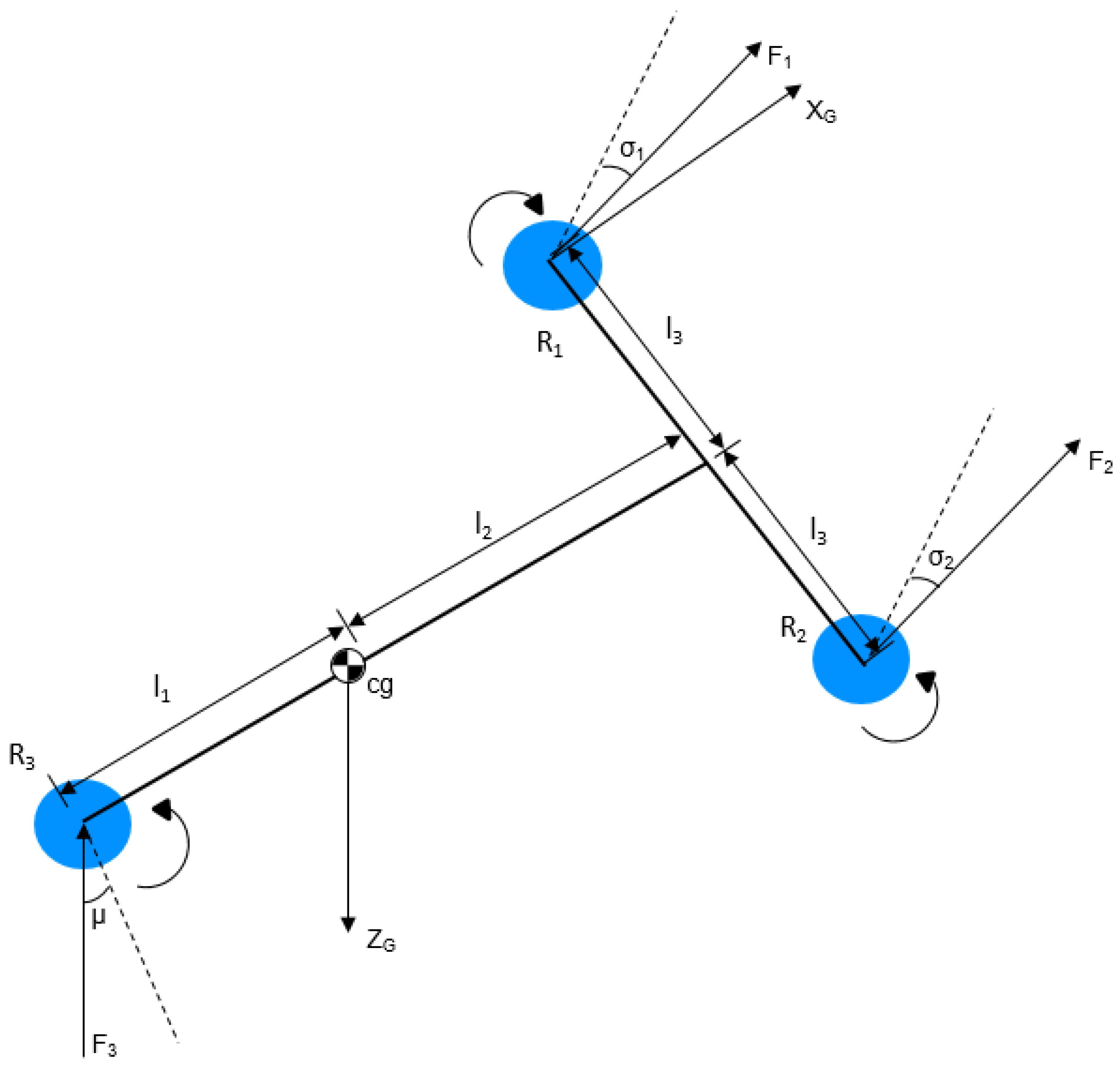
4.1. Description of the Tilt Tri-Rotor UAV

The vehicle under consideration is a hybrid of fixed-wing and rotary-wing UAVs. It comprises three rotors such that the placement of rotors at the end of each arm of the tilt-rotor tricopter forms a T-shaped structure, as shown in Figure 1. The three rotors can be tilted from 0° to 90° to realize the transition between hover and fixed-wing modes. These three rotors are labeled as $R_1,R_2$, and $R_3$, where ${\sigma }_1$, ${\sigma }_2$, and $\mu$ are the tilt angles of $R_1$, $R_2$, and $R_3$, respectively. $F_1,F_2$, and $F_3$ show the forces acting on each rotor, whereas $l_1$, $l_2$, and $l_3$ represent the moment arms.

The UAV can exhibit three flight modes: the hover mode, the fixed-wing mode, and the transition (from hover-to-cruise to cruise-to-hover) mode. A suitable hover mode controller must be designed to ensure the stability of the flight process and the precision of takeoff and landing during the takeoff and landing phases. A hybrid controller is usually employed in transition mode, which is made possible by the weight distribution of the hover mode controller and the fixed wing controller. The dynamic model has been developed based on the arrangement of rotors and the choice of coordinate system.

In the hover mode, the attitude is governed by two tilt angles and three rotational speeds. The right rotor ($R_2$) and the rear rotor ($R_3$) rotate in a counterclockwise direction, while the left rotor ($R_1$) rotates in a clockwise direction. The rear rotor helps compensate for the moment produced by the front rotors, stabilizing the pitch angle. When the aircraft is in transition mode, a gradual increase in forward velocity is attained with a gradual tilt of the two front rotors in the forward direction. However, the rear rotor decreases its rotational velocity. With the increase in speed, the tilt angles of both front rotors will reach 90 degrees. At this stage, the axes of these rotors coincide with the axis of the body of the UAV, and the third rotor stops completely. After achieving the desired height, the speed, at this moment, is enough to counteract gravity, and the tilt-rotor UAV turns into airplane mode (cruise) to fly like a conventional aircraft.

Table 1. Modeling parameters of tricopter.

Symbol	Description	Value	Unit
m	Mass of tricopter	1.5	kg
$l_1$	Moment arm	0.312	m
$l_2$	Moment arm	0.213	m
$l_3$	Moment arm	0.305	m
$I_{xx}$	Moment of inertia around x-body axis	0.0239	$\mathrm{kg}{\mathrm{m}}^2$
$I_{yy}$	Moment of inertia around y-body axis	0.01271	$\mathrm{kg}{\mathrm{m}}^2$
$I_{zz}$	Moment of inertia around z-body axis	0.01273	$\mathrm{kg}{\mathrm{m}}^2$

shows the modeling parameters of the tricopter.

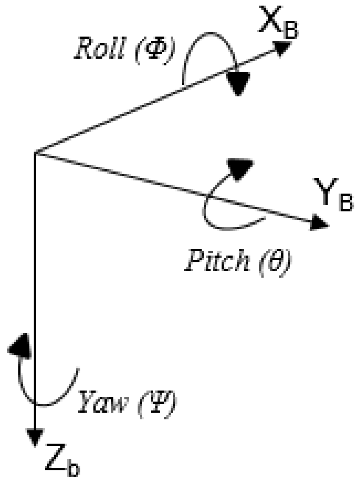
4.2. Coordinate System

The considered system can be defined using two different co-ordinate systems. The local coordinate system is denoted by B and can seen as the body-fixed coordinates of the tricopter. The global, denoted by G, is a coordinate system of earth or the inertial frame with its origin fixed to the center of mass ‘mg’ of the vehicle. The position of the respective tricopter UAV in an inertial frame is defined by coordinates X, Y, and Z.

The coordinate system can be seen in Figure 2. The $X_B$ axis is defined as the direction directly ahead, as seen from the tricopter’s perspective, and the $Y_B$ axis as the direction to the right. The $Z_B$ axis is established directly downward from the tricopter’s center of gravity. Using the rotation matrix R($\varphi ,\theta ,\psi$), the relationship between the coordinate systems of the earth and the tricopter (Body) may be mathematically explained. The attitude/rotation is defined by Euler angles, roll angle ($\varphi$), pitch angle ($\theta$), and yaw angle ($\psi$), and is the angle around $X_B$, $Y_B$, and $Z_B$ axes, respectively. A Direction Cosine Matrix (DCM) is used for their transformation from inertial (navigation) frame (X,Y,Z) to body frame ($X_b,Y_b,Z_b$), which is defined in Equation (1):

$$\left[\begin{array}{c}{X}_B\\ Y_B\\ Z_B\end{array}\right]=R(\varphi ,\theta ,\psi )\left[\begin{array}{c}X\\ Y\\ Z\end{array}\right]$$

(1)

where $R(\varphi ,\theta ,\psi )$ is the DCM or coordinate transformation matrix.

The rotation is applied to each of the three base vectors. The $Z_B$ axis is rotated first, with an angle of $\psi$, followed by the $Y_B$ axis, with an angle of $\theta$, and finally the $X_B$ axis, with an angle of $\varphi$ to produce the overall rotation. The rolling matrix $R(x,\varphi )$ along the x-axis, where $\varphi$ is the rolling angle along the x-axis, is as follows (Equation (2)):

$$R(x,\varphi )=\left[\begin{array}{ccc}1& 0& 0\\ 0& cos\varphi & sin\varphi \\ 0& -sin\varphi & cos\varphi \end{array}\right]$$

(2)

The rolling matrix $R(y,\theta )$ along the y-axis, where $\theta$ is the rolling angle along the y-axis, is as follows (Equation (3)):

$$R(y,\theta )=\left[\begin{array}{ccc}cos\theta & 0& -sin\theta \\ 0& 1& 0\\ sin\theta & 0& cos\theta \end{array}\right]$$

(3)

The rolling matrix $R(z,\psi )$ along the z-axis, where $\psi$ is the rolling angle along the z-axis, is given as (Equation (4)):

$$R(z,\psi )=\left[\begin{array}{ccc}cos\psi & sin\psi & 0\\ -sin\psi & cos\psi & 0\\ 0& 0& 1\end{array}\right]$$

(4)

Using the above-defined matrices, the coordinate transformation matrix can be calculated:

$$R(\varphi ,\theta ,\psi )=R(z,\psi )R(y,\theta )R(x,\varphi )$$

(5)

$$DCM=R(\varphi ,\theta ,\psi )=\left[\begin{array}{ccc}cos\theta cos\psi & cos\theta sin\psi & -sin\theta \\ sin\varphi sin\theta cos\psi -cos\varphi sin\psi & sin\varphi sin\theta sin\psi +cos\varphi cos\psi & sin\varphi cos\theta \\ cos\varphi sin\theta cos\psi +sin\varphi sin\psi & cos\varphi sin\theta sin\psi -sin\varphi cos\psi & cos\varphi cos\theta \end{array}\right]$$

(6)

The relation between Euler rates ($\dot{\varphi },\dot{\theta },\dot{\psi }$) in an inertial frame and angular body rates (p, q, r) can be represented as (Equation (7)):

$$\left[\begin{array}{c}\dot{\varphi }\\ \dot{\theta }\\ \dot{\psi }\end{array}\right]=\left[\begin{array}{ccc}1& sin\varphi tan\theta & cos\varphi tan\theta \\ 0& cos\varphi & -sin\varphi \\ 0& {\displaystyle \frac{sin\varphi }{cos\theta }}& {\displaystyle \frac{cos\varphi }{cos\theta }}\end{array}\right]\left[\begin{array}{c}p\\ q\\ r\end{array}\right]$$

(7)

4.3. Nonlinear Equations of Motion

This section focuses on deriving a 6-DOF nonlinear mathematical model of the tilt-rotor tricopter UAV. The schematic diagram of the tilt tri-rotor UAV coordinate system is shown in Figure 1. Dynamic pressure (Q) relies on two factors, aircraft speed (V) and air density ($\rho$), and is defined as:

$$Q={\displaystyle \frac{1}{2}}\rho V_a^2$$

(8)

Aerodynamic forces:

$$\left[\begin{array}{c}{F}_x\\ F_y\\ F_z\end{array}\right]=Q{S}_{ref}\left[\begin{array}{c}-C_{D_{\alpha }}cos\left(\alpha \right)+C_{L_{\alpha }}sin\left(\alpha \right)+(-C_{D_{\alpha }}cos\left(\alpha \right)+C_{L_{\alpha }}sin\left(\alpha \right)){\displaystyle \frac{c}{2V_a}}q\\ -C_{D_{\alpha }}sin\left(\alpha \right)-C_{L_{\alpha }}cos\left(\alpha \right)+(-C_{D_{\alpha }}sin\left(\alpha \right)-C_{L_{\alpha }}cos\left(\alpha \right)){\displaystyle \frac{c}{2V_a}}q\\ C_Y+C_{Y_{\beta }}\beta +{\displaystyle \frac{b}{2V_a}}p{C}_{Y_p}+{\displaystyle \frac{b}{2V_a}}r{C}_{Y_r}\end{array}\right]$$

(9)

Aerodynamic moments:

$$\left[\begin{array}{c}{M}_x\\ M_y\\ M_z\end{array}\right]=Q{S}_{ref}\left[\begin{array}{c}\overline{b}\left(C_L+C_{L_{\beta }}\beta +C_{L_p}{\displaystyle \frac{\overline{b}}{2V_a}}p+C_{L_r}{\displaystyle \frac{\overline{b}}{2V_a}}r\right)\\ c\left(C_M+C_{M_{\alpha }}+C_{M_q}{\displaystyle \frac{c}{2V_a}}q\right)\\ \overline{b}\left(C_N+C_{N_{\beta }}\left(\beta \right)+C_{N_p}{\displaystyle \frac{b}{2V_a}}p+C_{N_r}{\displaystyle \frac{b}{2V_a}}r\right)\end{array}\right]$$

(10)

Propulsive forces:

$$\left[\begin{array}{c}{F}_x\\ F_y\\ F_z\end{array}\right]=\left[\begin{array}{ccc}sin\left({\sigma }_1\right)& sin\left({\sigma }_2\right)& sin\left(\mu \right)\\ 0& 0& 0\\ -cos\left({\sigma }_1\right)& -cos\left({\sigma }_2\right)& -cos\left(\mu \right)\end{array}\right]\left[\begin{array}{c}{F}_1\\ F_2\\ F_3\end{array}\right]$$

(11)

Propulsive moments:

$$\left[\begin{array}{c}{M}_x\\ M_y\\ M_z\end{array}\right]=\left[\begin{array}{ccc}{l}_{3}cos\left({\sigma }_1\right)& -l_{3}cos\left({\sigma }_2\right)& 0\\ l_{1}cos\left({\sigma }_1\right)& l_{2}cos\left({\sigma }_2\right)& -l_{1}cos\left(\mu \right)\\ l_{3}sin\left({\sigma }_1\right)& -l_{3}sin\left({\sigma }_2\right)& sin\left(\mu \right)\end{array}\right]\left[\begin{array}{c}{F}_1\\ F_2\\ F_3\end{array}\right]+\left[\begin{array}{ccc}sin\left({\sigma }_1\right)& sin\left({\sigma }_2\right)& sin\left(\mu \right)\\ 0& 0& 0\\ -cos\left({\sigma }_1\right)& -cos\left({\sigma }_2\right)& -cos\left(\mu \right)\end{array}\right]\left[\begin{array}{c}-M_1\\ M_2\\ M_3\end{array}\right]$$

(12)

Gravitational forces:

$$\left[\begin{array}{c}{F}_x\\ F_y\\ F_z\end{array}\right]=\left[\begin{array}{c}-mgsin\left(\theta \right)\\ mgcos\left(\theta \right)sin\left(\varphi \right)\\ mgcos\left(\theta \right)cos\left(\varphi \right)\end{array}\right]$$

(13)

in which g is the gravity acceleration (g = 9.81 $\mathrm{m}/{\mathrm{s}}^2$ ).

The velocity ($V_b$) is given by Equation (14). Using components of velocity, incidence angle ($\alpha$), and sideslip angle ($\beta$) can be calculated (Equations (15) and (16)).

$$V=\sqrt{u^2+v^2+w^2}$$

(14)

$$\alpha =\mathrm{atan}2(w,u)$$

(15)

$$\beta =\mathrm{atan}2(v,u)$$

(16)

Under the assumption of considering the tricopter as a rigid body and neglecting the gyroscopic moments due to inertia from rotors, pitching moment due to tilted rotors, drag forces, and drag moments, the dynamics are defined by the general nonlinear 6-DOF equations of motion. Equation (17) shows the derived translational and rotational equations of motion for the respective UAV. The rigid body dynamics of the tri-rotor UAV are derived from Newton’s principles. The UAV is free to rotate and translate in three dimensions. The 6-DOF rigid body equations of motion for tri-rotor UAVs are expressed as differential equations in terms of translational motion, rotational motion, and kinematics.

$$\left.\begin{array}{c}\dot{u}=rv-qw-gsin\theta +{\displaystyle \frac{F_x}{m}}\hfill \\ \dot{v}=-r+pw+=gcos\theta sin\varphi +{\displaystyle \frac{F_y}{m}}\hfill \\ \dot{w}=qu-pv-gcos\theta cos\varphi +{\displaystyle \frac{F_z}{m}}\hfill \\ \dot{p}={\displaystyle \frac{I_{yy}-I_{zz}}{I_{xx}}}qr+{\displaystyle \frac{M_x}{I_{xx}}}\hfill \\ \dot{q}={\displaystyle \frac{I_{zz}-I_{xx}}{I_{yy}}}pr+{\displaystyle \frac{M_y}{I_{yy}}}\hfill \\ \dot{r}={\displaystyle \frac{I_{xx}-I_{yy}}{I_{zz}}}pq+{\displaystyle \frac{M_z}{I_{zz}}}\hfill \end{array}\right\}$$

(17)

where $F_x$, $F_y$, and $F_z$ are the external forces and $M_x$, $M_y$, and $M_z$ represent the external moments generated by the rotors in the x, y, and z directions, respectively. They all act on the center of gravity with respect to the body-fixed frame. The given equations demonstrate the dynamics in terms of translational velocities (u, v, w), rotational velocities (p, q, r), rotational angles ($\varphi ,\theta ,\psi$), and the rotational inertias ($I_{xx},I_{yy},I_{zz}$) of the tri-rotor UAV.

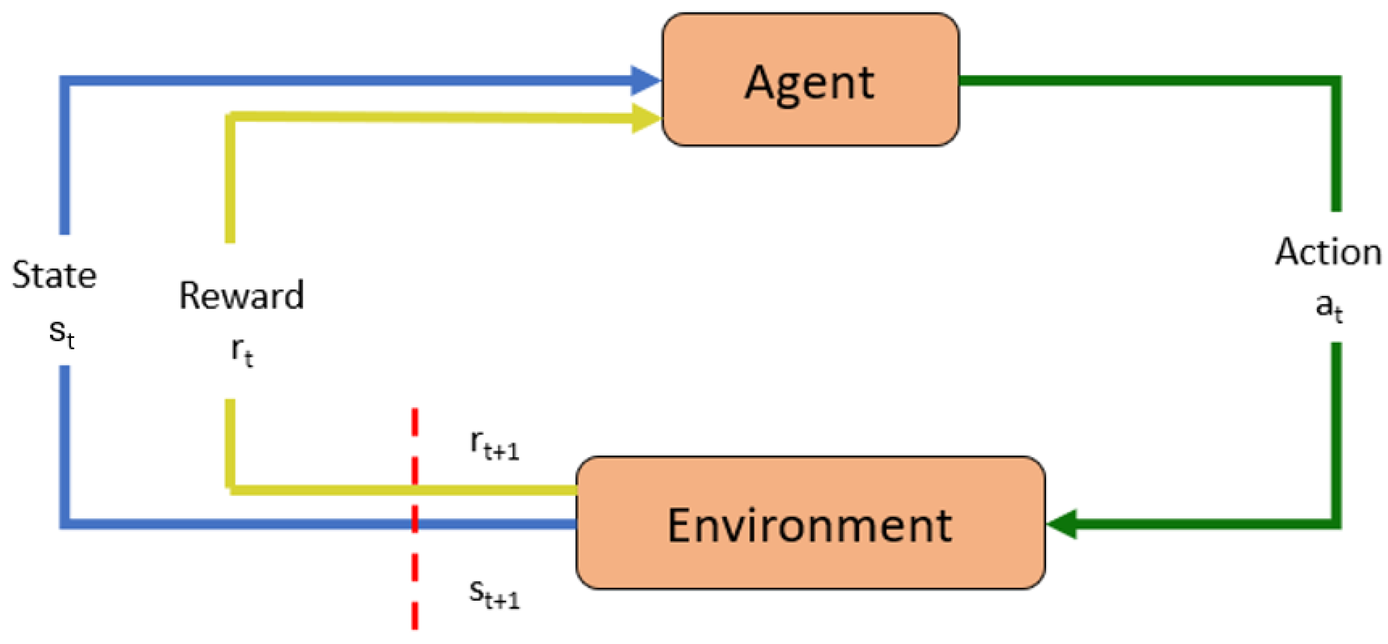
5. Reinforcement-Learning Framework

Reinforcement Learning (RL) is a specialized branch of machine learning that enables the agent to use experience to develop an ideal behavior. As described in [81], it is a learning framework where the agent learns via a trial and error method from its environment. Unlike other machine-learning algorithms, the agent/learner is not given a proper set of actions. It explores and learns from the environment to achieve the maximum rewards to reach a specific target or goal. Such algorithms differ from supervised learning as direct statistical pattern recognition cannot be applied to these problems. The simultaneous process of learning and zero a priori knowledge of the environment demands a better strategy. The sequence of actions is progressively improved, which helps to attain the best behavior/policy to reach the final goal.

The basic framework of reinforcement-learning algorithms consists of an agent that takes actions according to its state space in a particular environment and receives feedback to perform the defined task. Over time, the continuous agent–environment interaction leads to a maximized reward [7]. The agent, in its initial state, $s_t$, in the environment, acts, $a_t$, and, in return, receives a reward, $r_{t+1}$, to decide its following action to acquire the next state, $s_{t+1}$. This iterative approach follows a continually updating policy function to estimate its next move. This can be seen in Figure 3.

Another influence on RL is optimal control. In an RL environment, the agent, at each state, continuously learns from its experience and rewards (feedback) from the environment. This state is considered the environment’s statistics and consists of information the agent requires to take action, such as the position of sensors and actuators. This algorithm is policy-based and requires the agent to learn a policy (controlled strategy) $\pi$, which helps to maximize the cumulative but discounted reward. Hence, the RL agent solves the problem of optimal control. However, continuous learning from the environment challenges RL since a state transition dynamics model is unavailable in this technique. This method of RL can be formally described as the Markov Decision Process (MDP):

• A set of states, S, and a distribution of initial states, $\mathit{p}\left(s_o\right)$
• A set of actions, A
• Transition dynamics, T($s_{t+1}|s_t,a_t$)
• An instantaneous reward function, R($s_t,a_t,s_{t+1}$)
• A discount factor, $\gamma$∈ [0, 1]

Here, policy $\pi$ is a mapping of states to a probability distribution over actions: $\pi :\mathit{S}\to \mathit{p}(\mathit{A}=a|\mathit{S})$. Suppose the state is reset after each episode of length T (episodic). In that case, the sequence of actions, states, and rewards in the respective episode constitute a trajectory or rollout of the policy. This roll out of policy accumulates rewards from the environment for each episode, resulting in the return $R={\sum }_{t=0}^{T-1}{\gamma }^t{r}_{t+1}$. The optimal policy, ${\pi }^{*}$, is developed based on the maximum expected return from all states (Equation (18)):

$${\pi }^{*}=argma{x}_{\pi }E\left[R\right|\pi ]$$

(18)

For the non-episodic process, T = ∞. Here, $\gamma$ < 1 prevents the sum of rewards from being accumulated. Moreover, methods with finite transitions are applicable, whereas those relying on complete trajectories are not. The Markov property takes decisions for a state $s_t$ based only on the previous state, i.e., $s_{t-1}$, ignoring $\{s_0,s_1,\dots s_{t-2}\}$. This assumption becomes unrealistic as all the states should be fully observable. A modification of MDP is Partially Observable MDP (POMDP), where the distribution of observation depends on the current state and previous action [82]. A common approach to replace MDP is implementing Recurrent Neural Networks (RNNs) [51,83,84], which are dynamic systems, unlike feed-forward neural networks.

5.1. Deep-Reinforcement-Learning Algorithms

This section briefly covers the Deep Deterministic Policy Gradient (DDPG), Proximal Policy Optimization (PPO), and Trust Region Policy Optimization (TRPO) algorithms for maximizing the trajectory of the respective tilt-rotor tricopter UAV. These algorithms are used in Deep Reinforcement Learning (DRL) for their stability and efficiency in training agents to perform complex tasks.

These algorithms are implemented by setting up the necessary neural networks for policy and value functions, defining the state and action spaces, and designing an appropriate reward function. Their training involves interacting with a simulation environment to collect experiences and updating the respective networks based on observed rewards and policy improvements. Using these algorithms for UAV trajectory optimization provides robust and stable learning of control policies, crucial for performing precise and efficient hover-to-cruise maneuvers in tilt-rotor tricopter UAVs.

In general, DDPG is suitable for continuous action spaces with high-dimensional state space such as for controlling UAVs. However, it is sensitive to hyperparameter tuning and tends to get stuck in local optima, especially in complex environments. TRPO ensures monotonic updates in policy, which makes it robust towards large updates, but it has high computational costs and issues with stability. PPO strikes a balance between stability and efficiency, but it may face issues in fine tuning the complex UAV maneuvers. These RL-based methods face challenges during hover-to-cruise maneuvering, such as handling continuous state-action spaces, maintaining stability, and managing control inputs in an optimum manner.

During hover-to-cruise transition, the tricopter needs to maintain vertical thrust during hover mode and gradually transitions to forward thrust with the adjustment of tilt-rotors. The dynamic changes in speed and altitude require smooth adjustments in the speed and tilt angles of rotors. The algorithms under consideration need to cater the constraints on rotor speeds, tilt angles, energy consumption, and aerodynamic forces, etc. In the context of hover-to-cruise transition maneuvers for tilt-rotor UAVs, the control inputs (tilt angles and rotor speeds) are continuous variables; hence, DDPG is well suited for attitude and trajectory control. In real-world scenario where fine-tuning is necessary, DDPG can prove to be risky since it is more prone to overfitting and local optima issues, which makes it the least effective for complex transition maneuvering [47]. The guaranteed policy improvement of TRPO due to the factor of ‘trust region’ makes it more robust and stable when the UAV is transitioning from vertical takeoff to hover and then to cruise mode [52]. However, this stability requires enormous computational power, which makes it less practical, especially for real-time applications [83]. PPO is less sensitive to hyperparameters as compared to DDPG and is more sample efficient than TRPO. For the hover-to-cruise maneuver, this algorithm is more effective for balancing exploration and exploitation [85]. It is more adaptable and has a simpler objective function, but its reliance on this fixed function restricts it from fine tuning the parameters. PPO is recommended for real-time applications, but DDPG and TRPO might be useful in other contexts depending on the trade-offs between efficiency and stability.

5.2. Deep Deterministic Policy Gradient (DDPG)

The Deep Deterministic Policy Gradient (DDPG, Algorithm 1) algorithm is a model-free, off-policy Reinforcement-Learning (RL) algorithm well-suited for continuous action spaces, making it a practical choice for trajectory optimization in UAVs. The DDPG algorithm, introduced by Lillicrap et al. [47], combines the strengths of both DQN (Deep Q-Network) and actor–critic methods. It leverages the deterministic policy gradient algorithm to handle continuous action spaces directly, avoiding the need for action discretization. For many tasks, the action space becomes continuous. If such an action space is discretized too finely, it becomes enormous, making converging hard. DDPG is based on an actor–critic framework where the actor tunes a parameter, $\theta$, for policy function (best action space for a state) (Equation (19)) and the critic evaluates this function based on Temporal Difference (TD) error.

$${\pi }_{\theta }(s,a)=P\left[a\right|s,\theta ]$$

(19)

The agent employs two neural networks:

• Actor Network ($\mu (s\mid {\theta }^{\mu })$): Determines the best action, a, for a given state, s.
• Critic Network ($Q(s,a\mid {\theta }^Q)$): Evaluates action a given the state s.

The algorithm uses a target network for both the actor and the critic to improve stability during training. The deterministic target policy can be described as $\mu :S\to A$. These target networks are slowly updated to follow the original networks. The loss function for the critic network is defined in Equation (20), and the update for the actor network is given by Equation (21).

Critic Network Update:

$$L\left({\theta }^Q\right)=E_{s_t,a_t,r_t,s_{t+1}}\left[{\left(r_t+\gamma Q^{\prime }(s_{t+1},{\mu }^{\prime }(s_{t+1}\mid {\theta }^{{\mu }^{\prime }})\mid {\theta }^{Q^{\prime }})-Q(s_t,a_t\mid {\theta }^Q)\right)}^2\right]$$

(20)

where $Q^{\prime }$ and ${\mu }^{\prime }$ are the target networks for the critic and actor, respectively.

Actor Network Update:

$${\nabla }_{{\theta }^{\mu }}J\approx E_{s_t}\left[{\nabla }_{a}Q(s,a\mid {\theta }^Q){\mid }_{a=\mu (s\mid {\theta }^{\mu })}{\nabla }_{{\theta }^{\mu }}\mu (s\mid {\theta }^{\mu })\right]$$

(21)

The actor network is updated using the gradient of the Q-value function concerning the action.

In DDPG, Ornstein–Uhlenbeck noise (OU noise) is typically added to the action selection process to encourage exploration of the state space. The Ornstein–Uhlenbeck process is preferred because it generates temporally correlated noise, which is suitable for continuous control problems. The agent explores the environment more effectively, especially when the policy is not yet well-defined in the early stages of training. The noise is gradually reduced over time to allow for more deterministic behavior as the agent learns. The OU noise parameters (mean of the noise = 0.0, rate of mean aversion = 0.15, min value for noise scale = 0.2, max value for noise scale = 0.3, decay period = 100,000) are adjusted based on the specifics of the respective system and computational constraints.

Algorithm 1 DDPG (Deep Deterministic Policy Gradient)

1: Initialize the actor network $\mu \left(s\right|{\theta }^{\mu })$ and critic network $Q(s,a|{\theta }^Q)$ with random weights (${\theta }^{\mu }$ and ${\theta }^Q$).   2: Initialize target networks ${\mu }^{\prime }$ and $Q^{\prime }$ with weights ${\theta }^{{\mu }^{\prime }}\leftarrow {\theta }^{\mu }$ and ${\theta }^{Q^{\prime }}\leftarrow {\theta }^Q$.   3: Initialize replay buffer R.   4: repeat   5:     for each episode do   6:         Initialize a random process (Ornstein–Uhlenbeck noise) $\mathcal{N}$ for action exploration.   7:         Receive initial state $s_1$.   8:         for each timestep t do   9:            Select action $a_t=\mu \left(s_t\right|{\theta }^{\mu })+{\mathcal{N}}_t$. 10:            Execute action $a_t$, observe reward $r_t$ and next state $s_{t+1}$. 11:            Store transition $(s_t,a_t,r_t,s_{t+1})$ in replay buffer R. 12:            Sample a random mini-batch of N transitions $(s_i,a_i,r_i,s_{i+1})$ from R. 13:            Set $y_i=r_i+\gamma Q^{\prime }(s_{i+1},{\mu }^{\prime }\left(s_{i+1}\right|{\theta }^{{\mu }^{\prime }})|{\theta }^{Q^{\prime }})$. 14:            Update critic by minimizing the loss: $$L\left({\theta }^Q\right)={\displaystyle \frac{1}{N}}\sum _i{\left(y_i-Q(s_i,a_i|{\theta }^Q)\right)}^2.$$ 15:            Update actor using the sampled policy gradient: $${\nabla }_{{\theta }^{\mu }}J\approx {\displaystyle \frac{1}{N}}\sum _i{\nabla }_{a}Q(s,a|{\theta }^Q){|}_{a=\mu \left(s\right|{\theta }^{\mu })}{\nabla }_{{\theta }^{\mu }}\mu \left(s\right|{\theta }^{\mu }).$$ 16:            Update target networks: $${\theta }^{Q^{\prime }}\leftarrow \tau {\theta }^Q+(1-\tau ){\theta }^{Q^{\prime }}$$ $${\theta }^{{\mu }^{\prime }}\leftarrow \tau {\theta }^{\mu }+(1-\tau ){\theta }^{{\mu }^{\prime }}.$$ 17: until convergence

5.3. Proximal Policy Optimization (PPO)

PPO (Algorithm 2), introduced by Schulman et al. [85], is an on-policy algorithm designed to simplify and improve the training process by restricting the update size to keep new policies close to the old policies. A clip function is introduced to avoid divergence and reduce the difference between both policies. PPO balances sample efficiency and ease of implementation, making it a preferred choice for various RL applications.

This algorithm updates the parameter $\theta$ by computing the gradient through a Monte Carlo method. A policy loss function, J, is obtained when the agent interacts with the environment through such a policy. Practically, the parameters are updated through the backpropagation of these gradients in a neural network.

$${\nabla }_{\theta }J\left(\theta \right)=E_{\tau \sim {\pi }_{\theta }\left(\tau \right)}\left[\sum _t^T{\nabla }_{\theta }log{\pi }_{\theta }(a_t\mid s_t)·R\left(\tau \right)\right]$$

(22)

PPO uses Generalized Advantage Estimation (GAE) to reduce the variance of the gradient estimates and achieve a better policy. An advantage estimate is used, which is a function of the sum of discounted rewards ($r_{t^{\prime }}$) and the value function ($V_{\varphi }\left(s_t\right)$) for time steps $t^{\prime }>t$ discounted by $\gamma$.

$${\widehat{A}}^t=\sum _{t^{\prime }>t}{\gamma }^{t^{\prime }-t}(r_{t^{\prime }}-V_{\varphi }\left(s_t\right))$$

(23)

The advantage function assesses a behavior in relation to other behaviors in the state, rewarding good behavior with positive rewards and punishing bad behavior with negative rewards.

The PPO algorithm uses a surrogate objective function to ensure that updates do not deviate too much from the previous policy. This objective function is given by (Equation (24)):

$$L_{CLIP}\left(\theta \right)={\widehat{E}}_t\left[min\left(r_t\left(\theta \right){\widehat{A}}^t,\mathrm{clip}(r_t\left(\theta \right),1-ϵ,1+ϵ){\widehat{A}}^t\right)\right]$$

(24)

where $r_t\left(\theta \right)$ is the probability ratio between the new and old policies (Equation (25)), ${\widehat{A}}^t$ is the advantage estimate, and $ϵ$ is a hyperparameter with a small value that controls the clipping range by keeping the new policy close to the old policy.

$$r_t\left(\theta \right)={\displaystyle \frac{{\pi }_{\theta }(a_t\mid s_t)}{{\pi }_{{\theta }_{old}}(a_t\mid s_t)}}$$

(25)

Algorithm 2 PPO (Proximal Policy Optimization)

1: Initialize policy network ${\pi }_{\theta }\left(a\right|s)$ and value function $V_{\varphi }\left(s_t\right)$ with random weights.   2: Initialize target networks if using any.   3: Initialize hyperparameters: learning rate $\alpha$, clipping parameter $ϵ$, discount factor $\gamma$, and others as needed.   4: repeat   5:     for each iteration do   6:         Collect trajectories using the current policy ${\pi }_{\theta }$.   7:         Compute advantages ${\widehat{A}}_t$ using the collected trajectories and the value function estimates $V_{\varphi }\left(s_t\right)$.   8:         Update the policy by maximizing the PPO objective function: $$L_{CLIP}\left(\theta \right)=arg\underset{\theta }{max}\left[min\left(r_t\left(\theta \right)A_t,\mathrm{clip}\left(r_t\left(\theta \right),1-ϵ,1+ϵ\right)A_t\right)\right]$$   9:         Update the value function $V_{\varphi }$ by minimizing the value loss: $$V_{\varphi }=arg\underset{\varphi }{min}\left[{\left(V_{\varphi }\left(s_t\right)-{\widehat{V}}_t\right)}^2\right]$$ 10: until convergence

5.4. Trust Region Policy Optimization (TRPO)

TRPO (Algorithm 3), also introduced by Schulman et al. [52], is an on-policy algorithm that improves policy stability by ensuring that the updates do not drastically change the policy. This is achieved by constraining the step size in policy space. It is a policy optimization method that ensures updates are within a specific trust region, which helps maintain stability and improves performance. The TRPO algorithm optimizes the following objective function (Equation (26)) subject to a trust region constraint:

$$L_{TRPO}\left(\theta \right)=E_t\left[{\displaystyle \frac{{\pi }_{\theta }(a_t\mid s_t)}{{\pi }_{{\theta }_{old}}(a_t\mid s_t)}}{\widehat{A}}^t\right]$$

(26)

subject to:

$$E_t\left[D_{KL}\left[{\pi }_{{\theta }_{old}}(a_t\mid s_t)\mid \mid {\pi }_{\theta }(a_t\mid s_t)\right]\right]\le \delta$$

(27)

where $D_{KL}$ is the Kullback–Leibler divergence between the old and new policies and $\delta$ is a hyperparameter controlling the trust region size.

Algorithm 3 TRPO (Trust Region Policy Optimization)

1: Initialize policy parameters ${\theta }_0$, value function parameters ${\varphi }_0$, and policy network ${\pi }_{\theta }\left(a\right|s)$ with random weights. 2: Initialize hyperparameters: learning rate $\alpha$, maximum KL divergence $\delta$, discount factor $\gamma$. 3: repeat 4:     for each iteration do 5:         Collect trajectories using the current policy ${\pi }_{\theta }$. 6:         Compute advantages $A_t$ using the collected trajectories and the value function estimates $V_{\varphi }\left(s_t\right)$. 7:         Update the policy by optimizing the surrogate objective subject to a KL divergence constraint: $${\theta }_{\mathrm{new}}=L_{TRPO}\left(\theta \right)=E_t\left[{\displaystyle \frac{{\pi }_{\theta }(a_t\mid s_t)}{{\pi }_{{\theta }_{old}}(a_t\mid s_t)}}{\widehat{A}}^t\right]$$ such that $$E_t\left[D_{KL}\left[{\pi }_{{\theta }_{old}}(a_t\mid s_t)\mid \mid {\pi }_{\theta }(a_t\mid s_t)\right]\right]\le \delta$$ 8: until convergence

6. Simulation Environment

The simulation environment used for the transition maneuver and trajectory optimization of a tilt-rotor tricopter UAV using the three algorithms is implemented using MATLAB and Simulink (R2021b) for dynamic modeling and simulation. Reinforcement-learning libraries, including TensorFlow PyTorch and Reinforcement Learning Toolbox, implement the DDPG, PPO, and TRPO algorithms—Simulink’s built-in tools for modeling UAV dynamics and control systems.

7. Training Process

Implementing RL-based algorithms on a tilt-rotor tricopter to optimize the hover-to-cruise maneuver requires an action space, a state space, and a reward function. The state space includes relevant dynamic variables, the action space encompasses control inputs for maneuvering and mode transitions, and the reward shaping guides the learning process toward achieving efficient and safe flight operations. These components are crucial for designing a practical reinforcement-learning framework tailored to our research’s specific dynamics and objectives.

7.1. State Space

The state space comprises the collection of all the variables and parameters the UAV obtains from the environment. At any given time during the simulation, the position of the UAV relative to the inertial coordinate system and the motion variables are defined as state. The state space consists of position, velocity components (linear and angular velocities), orientation (roll, pitch, yaw angles), and tilt angle of rotors (${\sigma }_i$, where i = 1, 2).

$$\mathrm{state}=s={[x,y,z,u,v,w,\varphi ,\theta ,\psi ,p,q,r,{\sigma }_i]}^T$$

(28)

7.2. Action Space

In Reinforcement Learning (RL), the action space includes all possible actions the UAV can take at each time step in a given environment. These actions are controlled or adjusted by the policy learned by the respective algorithm being implemented. Values, such as rotor speeds, engine thrusts, and tilt angle, must be adjusted for a tilt-rotor tricopter UAV to transition from hover to cruise.

$$\mathrm{action}=a={[u_1,u_2,u_3,{\sigma }_i]}^T$$

(29)

7.3. Reward Function

A reward function assesses agents’ actions in the environment according to their current state. It defines the immediate feedback to the agent to determine its performance during simulation. It guides the learning process by reinforcing desirable behaviors and penalizing undesired ones. In this paper, reward function shaping involves setting up the function to guide the UAV toward achieving the desired maneuver efficiently. It should encourage the UAV to transition smoothly from hovering to cruising while optimizing performance criteria such as energy efficiency, stability, and minimal time to achieve a steady cruising speed.

7.4. Reward Function Components

a. Target Velocity Achievement: The agent should achieve and maintain a desired cruising velocity. It is modeled using the difference between the current and target velocities.

$$R_{\mathrm{velocity}}=-k_v\parallel v-v_{\mathrm{target}}\parallel$$

b. Minimized Energy Consumption: The agent optimizes the energy used during the maneuver and gets penalized for high energy consumption, which is represented by the throttle.

$$R_{\mathrm{energy}}=-k_{\mathrm{e}}·\sum _{i=1}^n{T}_i$$

where $T_i$ is the throttle level of rotor i, n is the number of rotors, and $k_e$ is a weight parameter for penalizing energy consumption.

c. Smooth Transition: This variable encourages a smooth and stable transition from hover to cruise by minimizing sudden changes in the tilt angles, $\Delta {\sigma }_i$, of the front two rotors.

$$R_{\mathrm{smoothness}}=-k_{\mathrm{sm}}·\sum _{i=1}^n\left(|\Delta {\sigma }_i|\right)$$

d. Stable Orientation: The stability reward, penalizing deviations in roll, pitch, and yaw, is expressed as:

$$R_{\mathrm{stability}}=-k_{\mathrm{st}}·\sum _{st=\varphi \theta \psi }\parallel e_{st}\parallel$$

$$R_{\mathrm{stability}}=-k_{\mathrm{st}}·\left(|\Delta \varphi |+|\Delta \theta |+|\Delta \psi |\right)$$

where $e_{st}$ includes the deviations in roll ($\Delta \varphi$), pitch ($\Delta \theta$), and yaw ($\Delta \varphi$).

e. Time Efficiency: The reward function that encourages timely completion of the maneuver is

$$R_{\mathrm{time}}=-k_{\mathrm{t}}·max(60-t_{elapsed},0)$$

where the maximum allowed time for completion of the maneuver is 60 and $t_{\mathrm{elapsed}}$ is the time elapsed since the start of the maneuver.

f. Safety Penalties: The reward function penalizing the UAV for approaching operational limits, including altitude, tilt angle, and thrust.

$$R_{\mathrm{safety}}=-k_{\mathrm{s}}·\sum _{j}max(0,{\mathrm{limit}}_j-{\mathrm{value}}_j)$$

These can be elaborated as

$$\begin{array}{ccc}\hfill R_{\mathrm{safety}}=-k_{\sigma }·\sum _{i=1}^{2}max(0,{\sigma }_i-{\sigma }_{\max })& \hfill -\hfill & k_T·\sum _{i=1}^{n}max(0,T_i-T_{\max })\hfill \\ \hfill -k_{hmin}·max(0,h_{\min }-h)& \hfill -\hfill & k_{hmax}·max(0,h-h_{\max })\hfill \end{array}$$

where $k_{\sigma }$, $k_T$, $k_{hmin}$, and $k_{hmax}$ are weighting factors for the respective penalties. ${\sigma }_i$ is the tilt angle for thre front two rotors, i, and ${\sigma }_{\max }$ is the maximum allowable tilt angle. It has a continuous value between 0° to 90°. h represents the current altitude, $h_{\min }$ is the minimum allowable altitude (1 m) to avoid ground collision and to maintain its cruising height, and $h_{\max }$ is the ceiling height of 12 m. $d_{\mathrm{obstacle}}$ is the distance to the nearest obstacle and $d_{\min }$ is the minimum safe distance from obstacles. The overall reward function is a weighted sum of the individual components, as shown in Equation (30), and the values for their weightage are given in

Table 2. Weights for reward function.

Weights	Values
$k_v$	0.1
$k_e$	0.7
$k_{sm}$	0.1
$k_{st}$	0.2
$k_t$	0.5
$k_{\sigma }$	0.2
$k_T$	0.5
$k_{hmin}$	0.6
$k_{hmax}$	0.1

.

$$r_t=R_{\mathrm{velocity}}+R_{\mathrm{energy}}+R_{\mathrm{smoothness}}+R_{\mathrm{stability}}+R_{\mathrm{time}}+R_{\mathrm{safety}}$$

(30)

The tilt-rotor tricopter acts as an RL agent. Initially, various parameters, including simulation duration, sample time, number of episodes, etc., are defined for each algorithm (

Table 3. Values of hyperparameters for each RL algorithm.

Hyper Parameters	DDPG	PPO	TRPO
Critic Learn Rate	1 × 10−3	1 × 10−4	-
Actor Learn Rate	1 × 10−4	1 × 10−4	-
Value Function Learning Rate	-	-	1 × 10−3
Sample Time	0.1	0.1	0.1
Experience buffer size (N)	1 × 106	-	-
Discount factor ($\gamma$)	0.99	0.997	0.99
Mini batch size (M)	64	128	128
Target update rate ($\tau$)	1 × 10−3	-	-
Target network update frequency (steps)	1000	-	-
KL-divergence limit ($\delta$)	-	0.01	0.01
Clip Factor	-	0.2	-
Generalised Advantage Estimation (${\lambda }_{GAE}$)	-	0.95	0.97

).

The system is operated at a sampling frequency of 10 Hz, ensuring accurate and responsive state updates. In MATLAB, the tic command was used to start timing and the toc command was used to measure the elapsed time for each cycle. To maintain the 10 Hz frequency, the elapsed time returned by the toc command was close to 0.1 s. This helped to verify if it aligns with the sampling frequency. Measuring the time taken per training step ensured that the algorithms were running at the correct rate (e.g., 10 Hz) by adjusting the simulation loop or model update rate accordingly. This approach was similar, regardless of the RL algorithm being used.

Control inputs were computed directly within Simulink based on the reinforcement-learning policy, and the UAV’s states were updated in real-time. The actor network is a neural network that determines the actions to be taken by the UAV based on the current state. In contrast, the critic network is a neural network that evaluates the actions taken by the actor network by estimating the Q-value, which represents the expected cumulative reward of taking a certain action in a given state.

For DDPG, the actor and critic networks have one hidden layer with 300 neurons and two with 100 neurons each. In an actor network, the first hidden layer of neurons takes the current state of the UAV as an input and performs computations using the ReLU activation function. The subsequent layers perform further computations. For the output layer, the action to be taken by the UAV is passed through an activation function of tanh to ensure it is within the acceptable range. In a critic network, the first hidden layer takes the concatenated state and action and performs computations to generate the Q-value, a scalar value representing the expected cumulative reward. All layers of the critic network use the ReLU rectifier.

The Generalized Advantage Estimation (GAE) method reduces the variance in critic output for PPO and TRPO. GAE introduces a hyperparameter (${\lambda }_{GAE}$) that controls the trade-off between reducing variance and maintaining low bias.

DDPG employs a replay buffer and target networks to stabilize training, while TRPO explicitly uses KL divergence to define a trust region. PPO approximates this concept through its clipped objective function, with optional KL divergence constraints in some implementations.

8. Results and Discussion

When the tilt-rotor tricopter UAV performed a vertical takeoff and transitioned from hover mode to cruise mode, flight dynamics and control algorithms, such as DDPG, PPO, and TRPO, influenced its position, velocity, and thrust trends.

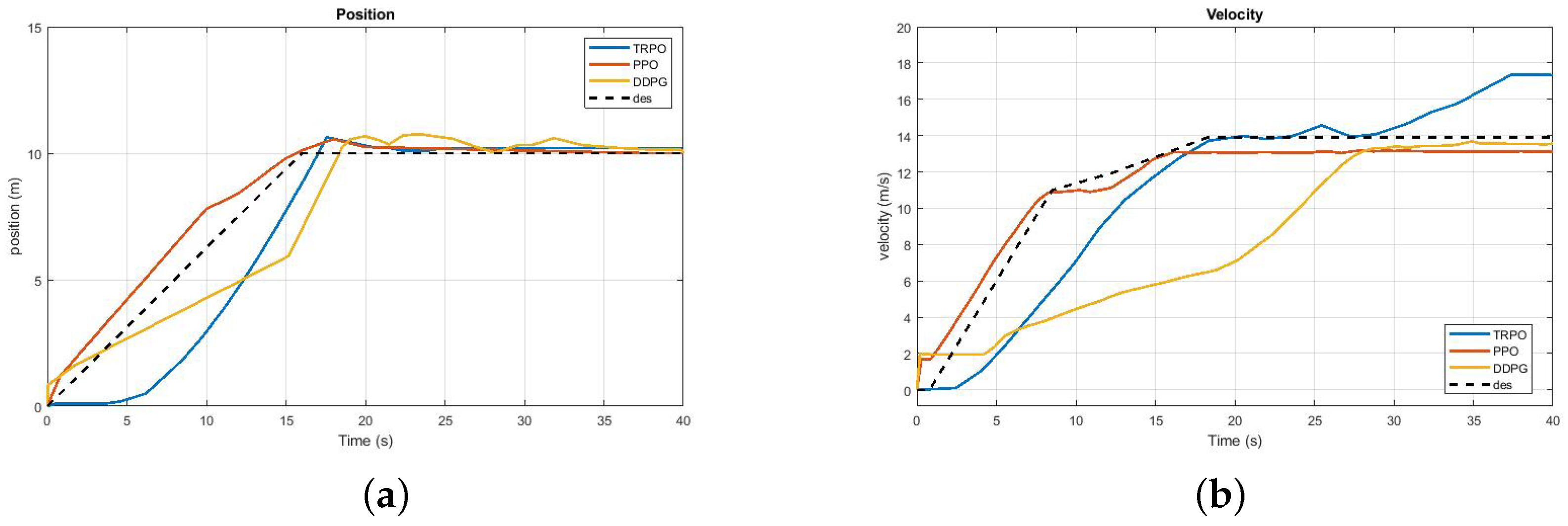
8.1. Trends of Position and Velocity of the UAV

In Figure 4a, it can be seen that, at the start of the vertical takeoff, the UAV’s position increases rapidly and it gains altitude until it reaches its desired height of 10 m. The UAV’s position on the z-axis stabilizes as it reaches a steady hover altitude. During the transition, the UAV’s position remains near the desired height (z-axis), but it will change more significantly in the horizontal plane as it accelerates to its cruising speed.

Initially, the UAV’s velocity starts to increase for a smooth takeoff. It tries to stabilize its value when the UAV cruises forward. This can be seen in Figure 4b.

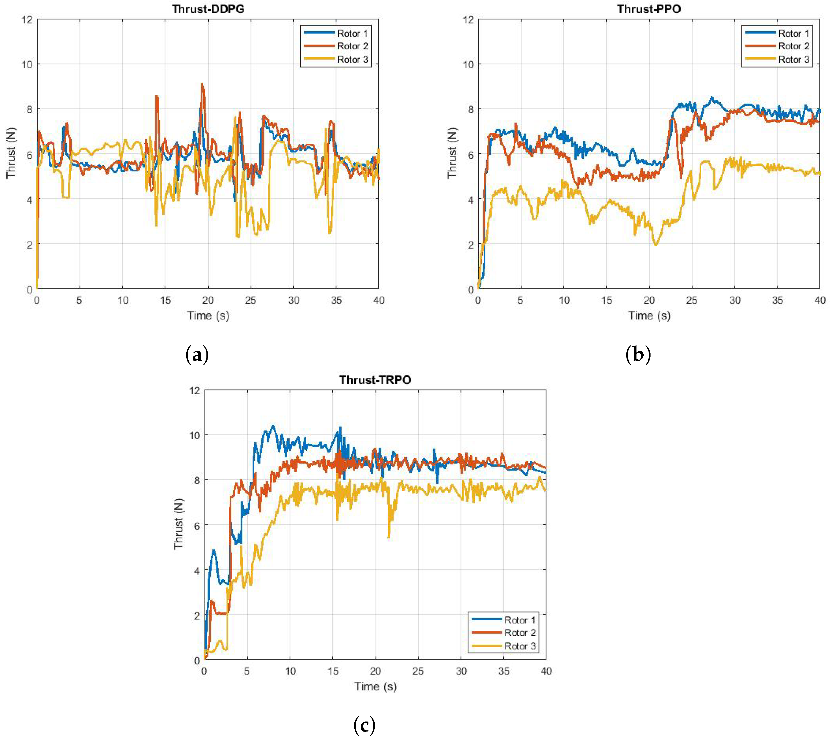
8.2. Control Variable of the UAV

The trend of thrust for the motors of tricopters starting off vertically and transitioning to cruise can be divided into two main phases: vertical takeoff and cruise transition. During the vertical takeoff phase, all motors need to generate enough thrust to overcome the weight of the tricopter and achieve takeoff. In Figure 5, it is observed that, initially, the motors generate a high level of thrust to lift the tricopter off the ground. It then tries to stabilize while maintaining a steady ascent and hover. As the tricopter transitions from vertical takeoff to forward cruise flight, the thrust dynamics change for the front and back rotors. The front rotors begin to tilt forward to transition from providing vertical lift to generating horizontal thrust for forward motion.

The tilt angle increases, progressively reducing the vertical lift component while increasing the horizontal thrust component. The back rotor reduces its thrust as the forward thrust from the front rotors takes over the primary role in generating forward motion. The thrust distribution among the motors is adjusted to maintain stability during the transition. This involves reducing the thrust on the rear engine and maintaining thrust on the forward motors to pitch the tricopter forward.

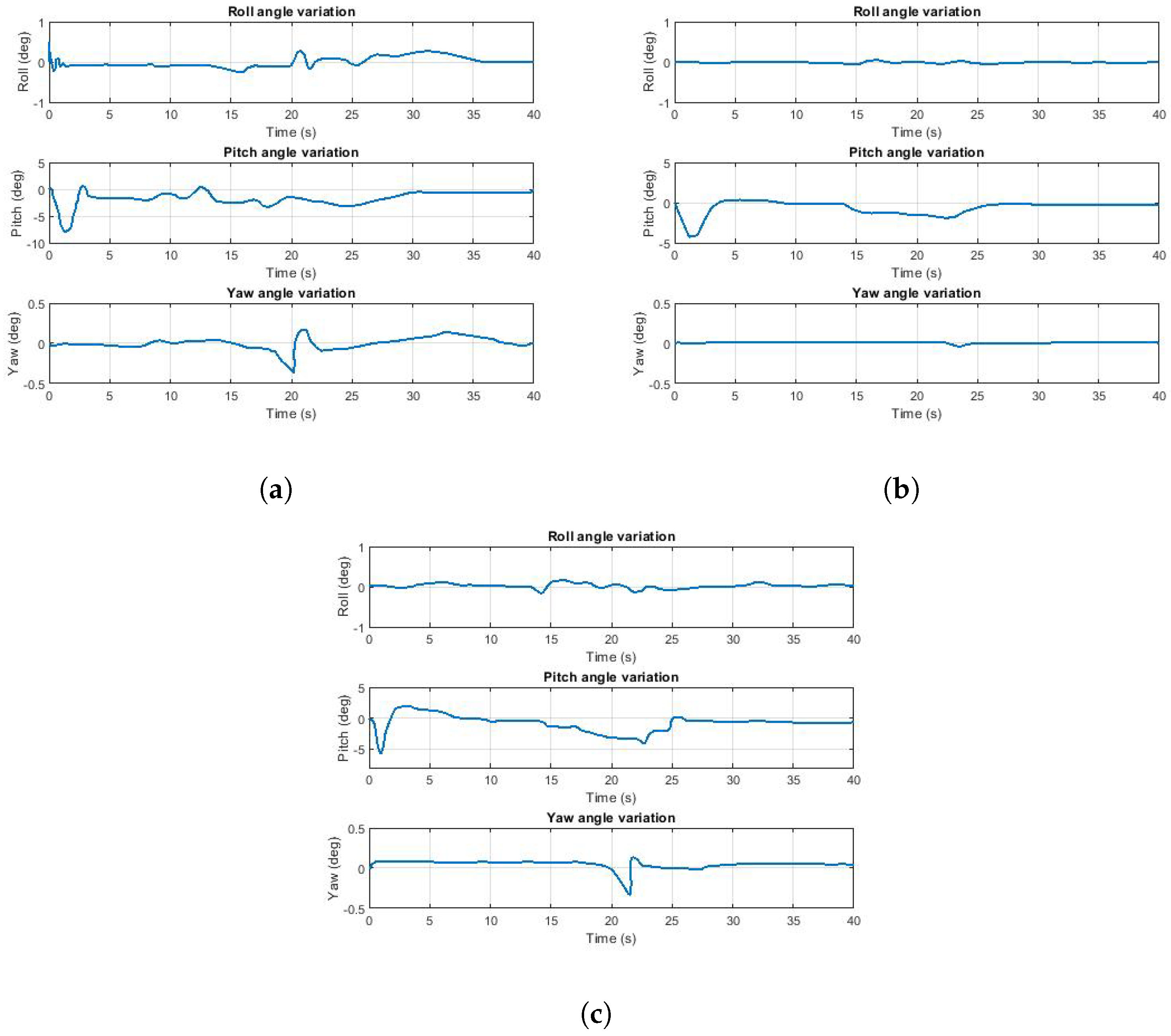
8.3. Trends of Euler Angles of the UAV

The trends of Euler angles (roll ($\varphi$), pitch ($\theta$), yaw ($\psi$)) provide insights into the behavior of the UAV during different phases of flight (Figure 6). During takeoff, the roll angle remains close to zero for all algorithms because the UAV is ascending vertically. The UAV tries to remain stable and close to zero, indicating level flight. During the transition, as seen in Figure 6a, the roll angle deviates from zero and tries to stabilize it, even after the transition. During takeoff and hover, the UAV tries to maintain its pitch and stabilize for a steady climb for all three algorithms. Only PPO performs well during the transition from hover to cruise, while the other two algorithms still show deviations. However, the UAV stabilized to a new steady-state value that was appropriate for cruise flight after some time. The yaw angle remained relatively constant during vertical takeoff and cruise, but the UAV faced difficulty in maintaining it during the transition; see Figure 6a,c.

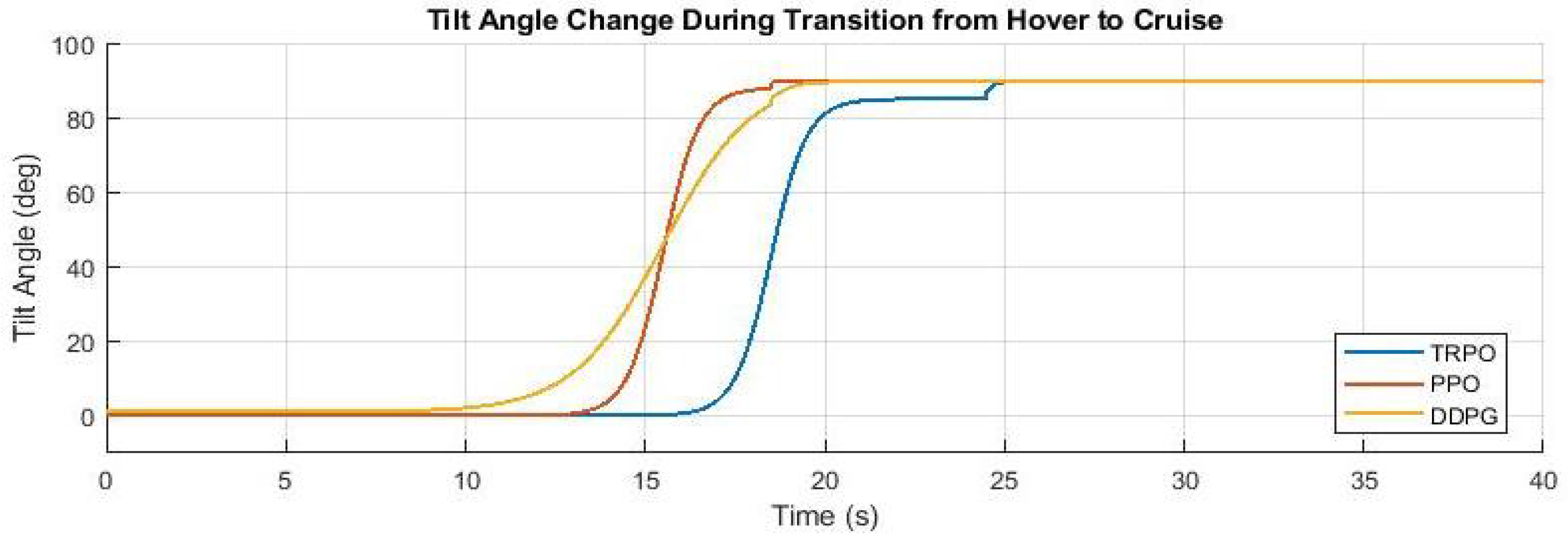
8.4. Variation of the Tilt Angle of Rotors of the UAV

In Figure 7, DDPG provides a smooth but potentially quicker transition due to its continuous control policy. PPO offers a steady and stable transition, minimizing oscillations, and TRPO ensures the most stable and conservative transition since it focuses on reliable and minor updates within a trust region. DDPG shows a trend that adapts quickly, potentially showing faster initial changes followed by a smoothing effect as it approaches the target. In contrast, in the case of PPO and TRPO, the tilt angle changes more steadily and slowly, ensuring that each change is within a safe and stable margin. The more gradual transitions shown for PPO and TRPO allow for smoother changes in aerodynamics and easier control of the UAV during the maneuver.

The plateau in each graph around the range of 80 degrees, followed by a continuation towards 90 degrees, can be attributed to several factors related to the UAV control dynamics and the implementation of the control algorithms. The control algorithms (especially in reinforcement learning) learn with step-wise adjustment. They learn a strategy to approach the maximum tilt angle in stages. The initial rapid increase could result from the learned policy optimizing for speed, while the brief plateau allows for a re-calibration before making the final adjustment. This can also be explained in terms of exploration and exploitation. This plateau results from balancing exploration (trying new actions) and exploitation (using known good actions). The algorithm temporarily exploits a near-optimal angle (around 80 degrees) before exploring further to reach the optimal tilt angle (90 degrees).

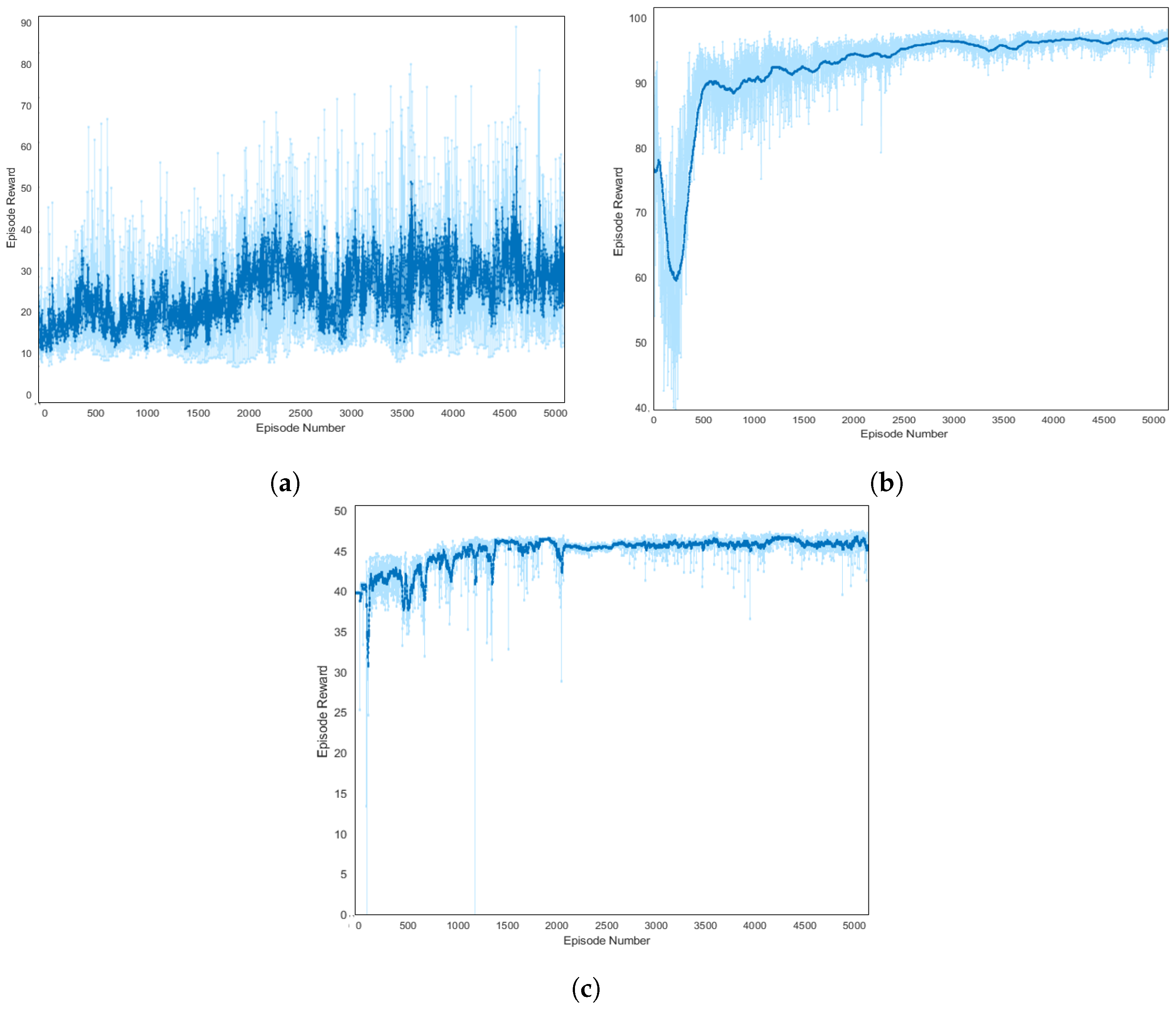
8.5. Learning of Algorithms

The differences between the three algorithms causes the agent (UAV) to learn and respond differently. This variation of implementation is explained as follows.

8.5.1. Deep Deterministic Policy Gradient (DDPG)

During takeoff, DDPG learns to control the thrust and pitch of the tilt-rotor to achieve a stable vertical takeoff. Learning the appropriate action sequences optimizes the transition from hover to cruise. It adapts to maintain steady cruising by balancing exploration and exploitation of the learned policy.

8.5.2. Proximal Policy Optimization (PPO)

PPO uses a clipped objective function to ensure stable learning, which helps control the UAV’s ascent during takeoff. It learns a policy that efficiently transitions from hover to cruise while ensuring smooth cruising by optimizing the policy to maintain the desired velocity and trajectory.

8.5.3. Trust Region Policy Optimization (TRPO)

TRPO focuses on optimizing the policy while ensuring that updates do not deviate significantly, which is beneficial for stable vertical takeoff. It handles the transition by maintaining a stable policy update. It optimizes the policy while respecting the trust region’s constraints.

Table 4. Comparative Summary of DDPG, TRPO, and PPO for trajectory planning.

Algorithm	Advantages	Disadvantages
DDPG	- High sample efficiency due to off-policy learning. - Suitable for continuous action spaces.	- Sensitive to hyperparameter tuning. - Prone to instability during training. - Requires careful exploration strategies to avoid local minima.
TRPO	- Monotonic policy improvement, ensures stability. - Effective in environments with significant nonlinearity and dynamics.	- High computational cost due to second-order optimization. - Less sample-efficient due to on-policy learning.
PPO	- Balances simplicity and performance with clipped objectives. - Computationally efficient. - Relatively robust to hyperparameter choices.	- Still less sample-efficient compared to off-policy methods. - May require extensive tuning to maximize performance.

summarizes the key strengths and weaknesses of the respective algorithms in the context of trajectory planning for the tilt-rotor UAV. The respective table highlights aspects such as sample efficiency, performance, stability, convergence, computational complexity, and robustness to hyperparameter tuning.

8.6. Reward Generation

In this study, the UAV trains for 5000 episodes for each algorithm. Sample time and simulation duration are predefined to determine the time for each episode. The algorithm calculates the reward for each episode and its average, as shown in Figure 8. For DDPG, at the beginning of the training phase the UAV explores the action space, and with each passing episode the experience replay buffer is filled, and the algorithm learns; see Figure 8a. Multiple experiments showed that a minimum of 1000 episodes is necessary for PPO to achieve effective convergence. In the case of TRPO, the agent learns and tries to maintain its rewards in a smaller window for better convergence.

The experimental results of average rewards and the number of steps required for the convergence of all algorithms are shown in

Table 5. Average rewards.

Parameters	DDPG	PPO	TRPO
Average reward	31.339	95.2336	46.8981
Episode Q0	174.8831	93.335	99.6194
No. of steps required for convergence		1600 ± 100	2100 ± 50

. In Table 5, it can be seen that the average reward of the PPO algorithm is the highest, followed by TRPO, while DDPG obtained the lowest. The PPO algorithm has the fastest convergence speed, which is nearly 30% faster than TRPO, while the DDPG algorithm can hardly converge; it can be deduced that the training efficiency of the PPO algorithm is faster than that of the others.

9. Conclusions

In this study, the reinforcement-learning method is adopted to train an agent to obtain optimal transition for the tilt-rotor VTOL aerial vehicles part of the design process. A mathematical model of the respective UAV, observation vector, action space, and reward function are also defined. The three RL-based algorithms, DDPG, PPO, and TRPO, are utilized to update the parameters of the neural network architecture. Simulation results successfully demonstrated the application of reinforcement-learning algorithms in enhancing the maneuverability and operational efficiency of a tilt-rotor tricopter UAV.

A comprehensive analysis of RL-based transition flight control algorithms are performed to evaluate the performance of the UAV. Among the algorithms tested, Proximal Policy Optimization (PPO) emerged as the most effective, outperforming Deep Deterministic Policy Gradient (DDPG) and Trust Region Policy Optimization (TRPO) in terms of stability, convergence speed, and adaptability to complex flight transitions. The superior performance of PPO underscores its potential as a robust solution for UAV control in dynamic environments, paving the way for more autonomous and efficient aerial systems.

References

1. Ol, M.; Parker, G.; Abate, G.; Evers, J. Flight controls and performance challenges for MAVs in complex environments. In Proceedings of the AIAA Guidance, Navigation and Control Conference and Exhibit, Honolulu, HI, USA, 18–21 August 2008; p. 6508. [Google Scholar]
2. Sababha, B.H.; Zu’bi, H.M.A.; Rawashdeh, O.A. A rotor-tilt-free tricopter UAV: Design, modelling, and stability control. Int. J. Mechatronics Autom. 2015, 5, 107–113. [Google Scholar] [CrossRef]
3. Logan, M.; Vranas, T.; Motter, M.; Shams, Q.; Pollock, D. Technology challenges in small UAV development. In Infotech@ Aerospace; ARC: Arlington, VA, USA, 2005; p. 7089. [Google Scholar]
4. Bolkcom, C. V-22 Osprey Tilt-Rotor Aircraft; Library of Congress Washington DC Congressional Research Service: Washington, DC, USA, 2004. [Google Scholar]
5. Ozdemir, U.; Aktas, Y.O.; Vuruskan, A.; Dereli, Y.; Tarhan, A.F.; Demirbag, K.; Erdem, A.; Kalaycioglu, G.D.; Ozkol, I.; Inalhan, G. Design of a commercial hybrid VTOL UAV system. J. Intell. Robot. Syst. 2014, 74, 371–393. [Google Scholar] [CrossRef]
6. Papachristos, C.; Alexis, K.; Tzes, A. Dual–authority thrust–vectoring of a tri–tiltrotor employing model predictive control. J. Intell. Robot. Syst. 2016, 81, 471–504. [Google Scholar] [CrossRef]
7. Chen, Z.; Jia, H. Design of flight control system for a novel tilt-rotor UAV. Complexity 2020, 2020, 4757381. [Google Scholar] [CrossRef]
8. Govdeli, Y.; Muzaffar, S.M.B.; Raj, R.; Elhadidi, B.; Kayacan, E. Unsteady aerodynamic modeling and control of pusher and tilt-rotor quadplane configurations. Aerosp. Sci. Technol. 2019, 94, 105421. [Google Scholar] [CrossRef]
9. Ningjun, L.; Zhihao, C.; Jiang, Z.; Yingxun, W. Predictor-based model reference adaptive roll and yaw control of a quad-tiltrotor UAV. Chin. J. Aeronaut. 2020, 33, 282–295. [Google Scholar]
10. Di Francesco, G.; Mattei, M.; D’Amato, E. Incremental nonlinear dynamic inversion and control allocation for a tilt rotor UAV. In Proceedings of the AIAA Guidance, Navigation, and Control Conference, National Harbor, MD, USA, 13–17 January 2014; p. 0963. [Google Scholar]
11. Kong, Z.; Lu, Q. Mathematical modeling and modal switching control of a novel tiltrotor UAV. J. Robot. 2018, 2018. [Google Scholar] [CrossRef]
12. Yildiz, Y.; Unel, M.; Demirel, A.E. Adaptive nonlinear hierarchical control of a quad tilt-wing UAV. In Proceedings of the 2015 IEEE European Control Conference (ECC), Linz, Austria, 15–17 July 2015; pp. 3623–3628. [Google Scholar]
13. Yoo, C.S.; Ryu, S.D.; Park, B.J.; Kang, Y.S.; Jung, S.B. Actuator controller based on fuzzy sliding mode control of tilt rotor unmanned aerial vehicle. Int. J. Control. Autom. Syst. 2014, 12, 1257–1265. [Google Scholar] [CrossRef]
14. Yin, Y.; Niu, H.; Liu, X. Adaptive neural network sliding mode control for quad tilt rotor aircraft. Complexity 2017, 2017, 7104708. [Google Scholar] [CrossRef]
15. Yang, Y.; Yan, Y. Neural network approximation-based nonsingular terminal sliding mode control for trajectory tracking of robotic airships. Aerosp. Sci. Technol. 2016, 54, 192–197. [Google Scholar] [CrossRef]
16. Song, Z.; Li, K.; Cai, Z.; Wang, Y.; Liu, N. Modeling and maneuvering control for tricopter based on the back-stepping method. In Proceedings of the 2016 IEEE Chinese Guidance, Navigation and Control Conference (CGNCC), Nanjing, China, 12–14 August 2016; pp. 889–894. [Google Scholar]
17. Crowther, B.; Lanzon, A.; Maya-Gonzalez, M.; Langkamp, D. Kinematic analysis and control design for a nonplanar multirotor vehicle. J. Guid. Control. Dyn. 2011, 34, 1157–1171. [Google Scholar] [CrossRef]
18. Lanzon, A.; Freddi, A.; Longhi, S. Flight control of a quadrotor vehicle subsequent to a rotor failure. J. Guid. Control. Dyn. 2014, 37, 580–591. [Google Scholar] [CrossRef]
19. Tran, H.K.; Chiou, J.S.; Nam, N.T.; Tuyen, V. Adaptive fuzzy control method for a single tilt tricopter. IEEE Access 2019, 7, 161741–161747. [Google Scholar] [CrossRef]
20. Mohamed, M.K.; Lanzon, A. Design and control of novel tri-rotor UAV. In Proceedings of the 2012 IEEE UKACC International Conference on Control, Cardiff, UK, 3–5 September 2012; pp. 304–309. [Google Scholar]
21. Kastelan, D.; Konz, M.; Rudolph, J. Fully actuated tricopter with pilot-supporting control. IFAC-PapersOnLine 2015, 48, 79–84. [Google Scholar] [CrossRef]
22. Servais, E.; d’Andréa Novel, B.; Mounier, H. Ground control of a hybrid tricopter. In Proceedings of the 2015 IEEE International Conference on Unmanned Aircraft Systems (ICUAS), Denver, CO, USA, 9–12 June 2015; pp. 945–950. [Google Scholar]
23. Kumar, R.; Sridhar, S.; Cazaurang, F.; Cohen, K.; Kumar, M. Reconfigurable fault-tolerant tilt-rotor quadcopter system. In Proceedings of the Dynamic Systems and Control Conference, Atlanta, GA, USA, 30 September–3 October 2018; American Society of Mechanical Engineers: New York, NY, USA, 2018; Volume 51913, p. V003T37A008. [Google Scholar]
24. Kumar, R.; Nemati, A.; Kumar, M.; Sharma, R.; Cohen, K.; Cazaurang, F. Tilting-rotor quadcopter for aggressive flight maneuvers using differential flatness based flight controller. In Proceedings of the Dynamic Systems and Control Conference, Tysons, VA, USA, 11–13 October 2017; American Society of Mechanical Engineers: New York, NY, USA, 2017; Volume 58295, p. V003T39A006. [Google Scholar]
25. Lindqvist, B.; Mansouri, S.S.; Agha-mohammadi, A.a.; Nikolakopoulos, G. Nonlinear MPC for collision avoidance and control of UAVs with dynamic obstacles. IEEE Robot. Autom. Lett. 2020, 5, 6001–6008. [Google Scholar] [CrossRef]
26. Wang, Q.; Namiki, A.; Asignacion Jr, A.; Li, Z.; Suzuki, S. Chattering reduction of sliding mode control for quadrotor UAVs based on reinforcement learning. Drones 2023, 7, 420. [Google Scholar] [CrossRef]
27. Jiang, B.; Li, B.; Zhou, W.; Lo, L.Y.; Chen, C.K.; Wen, C.Y. Neural network based model predictive control for a quadrotor UAV. Aerospace 2022, 9, 460. [Google Scholar] [CrossRef]
28. Raivio, T.; Ehtamo, H.; Hämäläinen, R.P. Aircraft trajectory optimization using nonlinear programming. In System Modelling and Optimization: Proceedings of the Seventeenth IFIP TC7 Conference on System Modelling and Optimization, 1995; Springer: Berlin/Heidelberg, Germany, 1996; pp. 435–441. [Google Scholar]
29. Betts, J.T. Survey of numerical methods for trajectory optimization. J. Guid. Control. Dyn. 1998, 21, 193–207. [Google Scholar] [CrossRef]
30. Judd, K.; McLain, T. Spline based path planning for unmanned air vehicles. In Proceedings of the AIAA Guidance, Navigation, and Control Conference and Exhibit, Montreal, QC, Canada, 6–9 August 2001; p. 4238. [Google Scholar]
31. Maqsood, A.; Go, T.H. Optimization of transition maneuvers through aerodynamic vectoring. Aerosp. Sci. Technol. 2012, 23, 363–371. [Google Scholar] [CrossRef]
32. Mir, I.; Maqsood, A.; Eisa, S.A.; Taha, H.; Akhtar, S. Optimal morphing–augmented dynamic soaring maneuvers for unmanned air vehicle capable of span and sweep morphologies. Aerosp. Sci. Technol. 2018, 79, 17–36. [Google Scholar] [CrossRef]
33. Feroskhan, M.; Go, T.H. Control strategy of sideslip perching maneuver under dynamic stall influence. Aerosp. Sci. Technol. 2018, 72, 150–163. [Google Scholar] [CrossRef]
34. Aggarwal, S.; Kumar, N. Path planning techniques for unmanned aerial vehicles: A review, solutions, and challenges. Comput. Commun. 2020, 149, 270–299. [Google Scholar] [CrossRef]
35. Sutton, R.S.; Barto, A.G. Reinforcement Learning: An Introduction; MIT Press: Cambridge, MA, USA, 2018. [Google Scholar]
36. Ma, Z.; Wang, C.; Niu, Y.; Wang, X.; Shen, L. A saliency-based reinforcement learning approach for a UAV to avoid flying obstacles. Robot. Auton. Syst. 2018, 100, 108–118. [Google Scholar] [CrossRef]
37. Liu, Y.; Liu, H.; Tian, Y.; Sun, C. Reinforcement learning based two-level control framework of UAV swarm for cooperative persistent surveillance in an unknown urban area. Aerosp. Sci. Technol. 2020, 98, 105671. [Google Scholar] [CrossRef]
38. Yan, C.; Xiang, X.; Wang, C. Fixed-Wing UAVs flocking in continuous spaces: A deep reinforcement learning approach. Robot. Auton. Syst. 2020, 131, 103594. [Google Scholar] [CrossRef]
39. Bengio, Y.; Courville, A.; Vincent, P. Representation learning: A review and new perspectives. IEEE Trans. Pattern Anal. Mach. Intell. 2013, 35, 1798–1828. [Google Scholar] [CrossRef] [PubMed]
40. Tesauro, G. Temporal difference learning and TD-Gammon. Commun. ACM 1995, 38, 58–68. [Google Scholar] [CrossRef]
41. Dahl, G.E.; Yu, D.; Deng, L.; Acero, A. Context-dependent pre-trained deep neural networks for large-vocabulary speech recognition. IEEE Trans. Audio Speech Lang. Process. 2011, 20, 30–42. [Google Scholar] [CrossRef]
42. Krizhevsky, A.; Sutskever, I.; Hinton, G.E. Imagenet classification with deep convolutional neural networks. In Proceedings of the Advances in Neural Information Processing Systems, Lake Tahoe, NV, USA, 3–6 December 2012; pp. 1097–1105. [Google Scholar]
43. Novati, G.; Mahadevan, L.; Koumoutsakos, P. Deep-Reinforcement-Learning for Gliding and Perching Bodies. arXiv 2018, arXiv:1807.03671. [Google Scholar]
44. Uhlenbeck, G.E.; Ornstein, L.S. On the theory of the Brownian motion. Phys. Rev. 1930, 36, 823. [Google Scholar] [CrossRef]
45. Zhu, C.; Byrd, R.H.; Lu, P.; Nocedal, J. Algorithm 778: L-BFGS-B: Fortran subroutines for large-scale bound-constrained optimization. Acm Trans. Math. Softw. 1997, 23, 550–560. [Google Scholar] [CrossRef]
46. Silver, D.; Huang, A.; Maddison, C.J.; Guez, A.; Sifre, L.; Van Den Driessche, G.; Schrittwieser, J.; Antonoglou, I.; Panneershelvam, V.; Lanctot, M.; et al. Mastering the game of Go with deep neural networks and tree search. Nature 2016, 529, 484. [Google Scholar] [CrossRef] [PubMed]
47. Lillicrap, T.P.; Hunt, J.J.; Pritzel, A.; Heess, N.; Erez, T.; Tassa, Y.; Silver, D.; Wierstra, D. Continuous control with deep reinforcement learning. arXiv 2015, arXiv:1509.02971. [Google Scholar]
48. Wei, E.; Wicke, D.; Luke, S. Hierarchical approaches for reinforcement learning in parameterized action space. In Proceedings of the 2018 AAAI Spring Symposium Series, Palo Alto, CA, USA, 26–28 March 2018. [Google Scholar]
49. dos Santos, S.R.; Barros, S.N.; Givigi, C.L.; Nascimento, L. Autonomous construction of multiple structures using learning automata: Description and experimental validation. IEEE Syst. J. 2015, 9, 1376–1387. [Google Scholar] [CrossRef]
50. Silver, D.; Lever, G.; Heess, N.; Degris, T.; Wierstra, D.; Riedmiller, M. Deterministic policy gradient algorithms. In Proceedings of the 31st International Conference on Machine Learning, PMLR, Beijing, China, 22–24 June 2014. [Google Scholar]
51. Hausknecht, M.; Stone, P. Deep recurrent q-learning for partially observable mdps. In Proceedings of the 2015 AAAI Fall Symposium Series, Palo Alto, CA, USA, 12–14 November 2015. [Google Scholar]
52. Schulman, J.; Levine, S.; Abbeel, P.; Jordan, M.; Moritz, P. Trust region policy optimization. In Proceedings of the International Conference on Machine Learning, Lille, France, 6–11 July 2015; pp. 1889–1897. [Google Scholar]
53. Hwangbo, J.; Sa, I.; Siegwart, R.; Hutter, M. Control of a quadrotor with reinforcement learning. IEEE Robot. Autom. Lett. 2017, 2, 2096–2103. [Google Scholar] [CrossRef]
54. Heess, N.; TB, D.; Sriram, S.; Lemmon, J.; Merel, J.; Wayne, G.; Tassa, Y.; Erez, T.; Wang, Z.; Eslami, S.; et al. Emergence of locomotion behaviours in rich environments. arXiv 2017, arXiv:1707.02286. [Google Scholar]
55. Lopes, G.C.; Ferreira, M.; da Silva Simões, A.; Colombini, E.L. Intelligent control of a quadrotor with proximal policy optimization reinforcement learning. In Proceedings of the 2018 IEEE Latin American Robotic Symposium, 2018 Brazilian Symposium on Robotics (SBR) and 2018 Workshop on Robotics in Education (WRE), Joao Pessoa, Brazil, 6–10 November 2018; pp. 503–508. [Google Scholar]
56. Bøhn, E.; Coates, E.M.; Moe, S.; Johansen, T.A. Deep reinforcement learning attitude control of fixed-wing uavs using proximal policy optimization. In Proceedings of the 2019 IEEE International Conference on Unmanned Aircraft Systems (ICUAS), Atlanta, GA, USA, 11–14 June 2019; pp. 523–533. [Google Scholar]
57. Koch, W.; Mancuso, R.; West, R.; Bestavros, A. Reinforcement learning for UAV attitude control. ACM Trans. Cyber-Phys. Syst. 2019, 3, 1–21. [Google Scholar] [CrossRef]
58. Deshpande, A.M.; Kumar, R.; Minai, A.A.; Kumar, M. Developmental reinforcement learning of control policy of a quadcopter UAV with thrust vectoring rotors. In Proceedings of the Dynamic Systems and Control Conference; American Society of Mechanical Engineers: Atlanta, GA, USA, 2020; Volume 84287, p. V002T36A011. [Google Scholar]
59. LaValle, S.M. Planning Algorithms; Cambridge University Press: Cambridge, UK, 2006. [Google Scholar]
60. Çakici, F.; Leblebicioğlu, M.K. Control system design of a vertical take-off and landing fixed-wing UAV. IFAC-PapersOnLine 2016, 49, 267–272. [Google Scholar] [CrossRef]
61. Saeed, A.S.; Younes, A.B.; Islam, S.; Dias, J.; Seneviratne, L.; Cai, G. A review on the platform design, dynamic modeling and control of hybrid UAVs. In Proceedings of the 2015 IEEE International Conference on Unmanned Aircraft Systems (ICUAS), Denver, CO, USA, 9–12 June 2015; pp. 806–815. [Google Scholar]
62. Chana, W.F.; Coleman, J.S. World’s first vtol airplane convair/navy xfy-1 pogo. In SAE Transactions; SAE International: Warrendale PA, USA, 1996; pp. 1261–1266. [Google Scholar]
63. Smith Jr, K.; Belina, F. Small V/STOL Aircraft Analysis, Volume 1; NASA: Greenbelt, MD, USA, 1974. [Google Scholar]
64. Ahn, O.; Kim, J.; Lim, C. Smart UAV research program status update: Achievement of tilt-rotor technology development and vision ahead. In Proceedings of the 27th Congress of International Council of the Aeronautical Sciences, Nice, France, 19–24 September 2010; pp. 2010–2016. [Google Scholar]
65. Pines, D.J.; Bohorquez, F. Challenges facing future micro-air-vehicle development. J. Aircr. 2006, 43, 290–305. [Google Scholar] [CrossRef]
66. Van Nieuwstadt, M.J.; Murray, R.M. Rapid hover-to-forward-flight transitions for a thrust-vectored aircraft. J. Guid. Control. Dyn. 1998, 21, 93–100. [Google Scholar] [CrossRef]
67. Stone, R.H.; Anderson, P.; Hutchison, C.; Tsai, A.; Gibbens, P.; Wong, K. Flight testing of the T-wing tail-sitter unmanned air vehicle. J. Aircr. 2008, 45, 673–685. [Google Scholar] [CrossRef]
68. Green, W.E.; Oh, P.Y. A MAV that flies like an airplane and hovers like a helicopter. In Proceedings of the Proceedings, 2005 IEEE/ASME International Conference on Advanced Intelligent Mechatronics, Monterey, CA, USA, 24–28 July 2005; pp. 693–698. [Google Scholar]
69. Green, W.E.; Oh, P.Y. Autonomous hovering of a fixed-wing micro air vehicle. In Proceedings of the Proceedings 2006 IEEE International Conference on Robotics and Automation, 2006, ICRA 2006, Orlando, FL, USA, 15–19 May 2006; pp. 2164–2169. [Google Scholar]
70. Green, W.E. A Multimodal Micro Air Vehicle for Autonomous Flight in Near-Earth Environments; Drexel University: Philadelphia, PA, USA, 2007. [Google Scholar]
71. Xili, Y.; Yong, F.; Jihong, Z. Transition flight control of two vertical/short takeoff and landing aircraft. J. Guid. Control. Dyn. 2008, 31, 371–385. [Google Scholar] [CrossRef]
72. Yanguo, S.; Huanjin, W. Design of flight control system for a small unmanned tilt rotor aircraft. Chin. J. Aeronaut. 2009, 22, 250–256. [Google Scholar] [CrossRef]
73. Muraoka, K.; Okada, N.; Kubo, D.; Sato, M. Transition flight of quad tilt wing VTOL UAV. In Proceedings of the 28th Congress of the International Council of the Aeronautical Sciences, Brisbane, Australia, 23–28 September 2012; pp. 3242–3251. [Google Scholar]
74. Mehra, R.; Wasikowski, M.; Prasanth, R.; Bennett, R.; Neckels, D. Model predictive control design for XV-15 tilt rotor flight control. In Proceedings of the AIAA Guidance, Navigation, and Control Conference and Exhibit, Montreal, QC, Canada, 6–9 August 2001; p. 4331. [Google Scholar]
75. Hameed, R.; Maqsood, A.; Hashmi, A.; Saeed, M.; Riaz, R. Reinforcement learning-based radar-evasive path planning: A comparative analysis. Aeronaut. J. 2022, 126, 547–564. [Google Scholar] [CrossRef]
76. dos Santos, S.R.B.; Nascimento, C.L.; Givigi, S.N. Design of attitude and path tracking controllers for quad-rotor robots using reinforcement learning. In Proceedings of the 2012 IEEE Aerospace Conference, Big Sky, MT, USA, 3–10 March 2012; pp. 1–16. [Google Scholar]
77. Wang, C.; Wang, J.; Shen, Y.; Zhang, X. Autonomous navigation of UAVs in large-scale complex environments: A deep reinforcement learning approach. IEEE Trans. Veh. Technol. 2019, 68, 2124–2136. [Google Scholar] [CrossRef]
78. Kohl, N.; Stone, P. Policy gradient reinforcement learning for fast quadrupedal locomotion. In Proceedings of the IEEE International Conference on Robotics and Automation, New Orleans, LA, USA, 26 April–1 May 2004; Proceedings. ICRA’04. 2004. IEEE: New York, NY, USA, 2004; Volume 3, pp. 2619–2624. [Google Scholar]
79. Ng, A.Y.; Coates, A.; Diel, M.; Ganapathi, V.; Schulte, J.; Tse, B.; Berger, E.; Liang, E. Autonomous inverted helicopter flight via reinforcement learning. In Experimental Robotics IX; Springer: Berlin/Heidelberg, Germany, 2006; pp. 363–372. [Google Scholar]
80. Strehl, A.L.; Li, L.; Wiewiora, E.; Langford, J.; Littman, M.L. PAC model-free reinforcement learning. In Proceedings of the 23rd International Conference on Machine Learning; Association for Computing Machinery: New York, NY, USA, 2006; pp. 881–888. [Google Scholar]
81. Wood, C. The flight of albatrosses (a computer simulation). Ibis 1973, 115, 244–256. [Google Scholar] [CrossRef]
82. Kaelbling, L.P.; Littman, M.L.; Cassandra, A.R. Planning and acting in partially observable stochastic domains. Artif. Intell. 1998, 101, 99–134. [Google Scholar] [CrossRef]
83. Mnih, V.; Badia, A.P.; Mirza, M.; Graves, A.; Lillicrap, T.; Harley, T.; Silver, D.; Kavukcuoglu, K. Asynchronous methods for deep reinforcement learning. In Proceedings of the International Conference on Machine Learning, New York, NY, USA, 19–24 June 2016; pp. 1928–1937. [Google Scholar]
84. Wierstra, D.; Förster, A.; Peters, J.; Schmidhuber, J. Recurrent policy gradients. Log. J. Igpl 2010, 18, 620–634. [Google Scholar] [CrossRef]
85. Schulman, J.; Wolski, F.; Dhariwal, P.; Radford, A.; Klimov, O. Proximal policy optimization algorithms. arXiv 2017, arXiv:1707.06347. [Google Scholar]
Figure 1. Configuration of tilt-rotor tricopter.
Aerospace 11 01040 g001
Figure 2. Coordinate system.
Aerospace 11 01040 g002
Figure 3. Architecture of reinforcement learning.
Aerospace 11 01040 g003
Figure 4. (a) Height attained by UAV for all three algorithms. (b) Velocity of UAV for all three algorithms.
Aerospace 11 01040 g004
Figure 5. Thrust for all three rotors of the UAV: (a) DDPG; (b) PPO; (c) TRPO.
Aerospace 11 01040 g005
Figure 6. Euler angles of UAV during the maneuver: (a) DDPG; (b) PPO; (c) TRPO.
Aerospace 11 01040 g006
Figure 7. Change in tilt angles.
Aerospace 11 01040 g007
Figure 8. Episode reward received by the UAV during the training phase: (a) DDPG; (b) PPO; (c) TRPO.
Aerospace 11 01040 g008