Communication

Mathematical Mechanism of Gini Index Used for Multiple-Impulse Phenomenon Characterization

1
School of Missile Engineering, Rocket Force University of Engineering, Xi’an 710025, China
2
School of Mechanics, Civil Engineering and Architecture, Northwestern Polytechnical University, Xi’an 710072, China
3
Guangzhou Institute of Science and Technology, Guangzhou 510540, China
*
Authors to whom correspondence should be addressed.
Aerospace 2024, 11(12), 1034; https://doi.org/10.3390/aerospace11121034
Submission received: 27 September 2024 / Revised: 27 November 2024 / Accepted: 27 November 2024 / Published: 18 December 2024

Abstract

:
The Gini index (GI) is widely used for measuring the sparsity of signals and has been proven to be effective in the extraction of fault features. A fault-induced vibration, which involves the obvious phenomenon of multiple impulses, is a kind of sparse signal and the GI has been widely used in the diagnosis of rotating machine faults. However, why the GI can be used to evaluate the sparsity or impulsiveness of a signal has not been revealed directly. In this study, the mathematical mechanism of the GI, used for the representation of the multiple-impulse phenomenon, is deeply researched based on the theoretical deviation of the GI with regard to several typical signals. The theoretical results show that the GI increases with the increment in the number of impulses in the signal when the signal is interrupted by relatively low degrees of white noise. The bigger the difference between the amplitude of the impulse and the variance in the noise, the bigger the value of the GI. Namely, the signal-to-noise ratio has a great influence on the value of the GI. However, the GI is still a powerful tool for the characterization of the impulsive intensity of the multiple-impulse phenomenon. Both simulation and experimental data analysis are introduced to show the application of the GI in practice. It is shown that the fault diagnosis method based on the maximization of the GI is more powerful than that of kurtosis in terms of the extraction of fault features of rolling element bearings (REBs).

1. Introduction

Initially introduced in economics, the GI was originally used to measure inequality in terms of people’s income and wealth [1]. Recently, the GI has been widely used as a measure of sparsity in the machinery fault diagnosis process [2,3,4,5,6,7,8,9,10]. In particular, it has been proven to be powerful when used for depressing random impulsive noise during the fault diagnosis of rotating machines, such as REBs and gears [5,6,9,11]. For example, Miao et al. [12] developed improved kurtosis-guided grams, such as the Kurtogram [4], Protrugram [5] and SKRgram [6], via the GI for REB fault identification and later proposed a practical framework for the GI based on the squared envelope of vibration [2,3]. In 2024, Tong et al. [13] proposed a novel gear fault diagnosis method by using the spectral GI and segmented energy spectrum. Yu and Zhao [14] proposed a fault characteristic impulse separation method for flexible thin-wall bearings based on wavelet transform and the correlated GI. Chen et al. [15] developed a novel method, named the IGIgram, based on envelope analysis for REB fault diagnosis. The results showed that the GI family has quite good performance in the field of mechanical fault diagnosis. Moreover, many new indexes, such as the spectral GI [12] and correlated GI [14], have been developed based on the definition of the GI.
However, why the GI is useful for characterizing the fault features of mechanical components, such as REBs and gears, is not clearly stated in the existing literature. Namely, the mathematical mechanism of the GI, used to represent the impulse features of vibration signals, has not been discussed yet. Generally, the GI is used to measure the sparsity of a signal, and the fault-induced vibrations in REBs and gears are a kind of cyclical series of impulses, whose cyclical frequency is related to the location of the fault. Moreover, a cyclical series of impulses is a kind of multiple-impulse phenomenon and is a kind of sparse signal. In this case, we focused on revealing the mathematical mechanism of the GI for the representation of the multiple-impulse phenomenon, and the theoretical deviations of the GI in regard to several typical signals, including constant signals, an ideal series of cyclical impulses, white noise, white noise with a positive bias, and a series of cyclical impulses with white noise, have been researched in this paper. The theoretical results show that the GI increases with the increment in the number of impulses in the signal when the signal is interrupted by relatively low degrees of white noise. The bigger the difference between the amplitude of the impulse and the variance in the noise, the bigger the value of the GI. Simulations were performed to validate the correction of the theoretical deviation. Two experimental signal analyses were used to show the application of the GI in engineering.

2. Definition of GI

For an arbitrary signal x > 0, the discrete form of the signal can be represented as x n , n = 1 , N , where N is the length of the signal. Denoting the GI with γ , the GI is defined based on the discrete form of the signal and is given by [3]
γ = 1 2 n = 1 N x n x 1 N n + 1 / 2 N ,   x n 0 ,      
where x 1 = n = 1 N x n is the l 1 norm of the signal and x n , n = 1 , N denotes the order statistic variable of x n , n = 1 , N , namely x 1 < x 2 < < x N 1 < x N . x k denotes the kth-order statistic variable of x n , n = 1 , N .
Denoting α n = 2 N n + 1 / 2 N , n = 1 , , N , then Equation (1) can be further denoted as
                      γ = 1 2 x 1 n = 1 N x n N n + 1 / 2 N       = 1 2 n = 1 N x n n = 1 N x n N n + 1 / 2 N = 1 n = 1 N α n x n n = 1 N x n ,       x n 0   ,          
where n = 1 N α n = N . It can be seen that the GI is related to the ratio of the weighted summation of the order statistic variable to the summation of the variable. Figure 1 illustrates the coefficient α n when the length of the series equals 2000. Obviously, the coefficient α n decreases linearly to 0 and the summation of α n equals the area under the line of α n .

3. GI of Typical Signals

To understand why the GI is powerful for characterizing the impulsiveness or sparsity of the fault-induced vibration and is robust to the random impulsive noise, the GIs of several typical signals are theoretically calculated in this section. Only the discrete forms of the signal are considered because the GI is defined based on the discrete signal.

3.1. Constant Signal

Suppose that an arbitrary non-zero constant signal is denoted as x n = c , c 0 , n = 1 , . . . , N . It is very easy to obtain corresponding order statistic series, namely x n = c , n = 1 , . . . , N . In this case, the GI of the constant signal is given by
γ = 1 n = 1 N α n x n n = 1 N x n = 1 n = 1 N α n c n = 1 N c = 1 n = 1 N α n c N c = 1 c n = 1 N α n N c = 0   .    
We use the equation n = 1 N α n = N in the last equation. It can be seen that the GI of the constant signal equals zero. This means that there is no impulsive characteristic in the non-zero constant signal or that the non-zero constant signal is not sparse.

3.2. Ideal Series of Cyclical Impulses
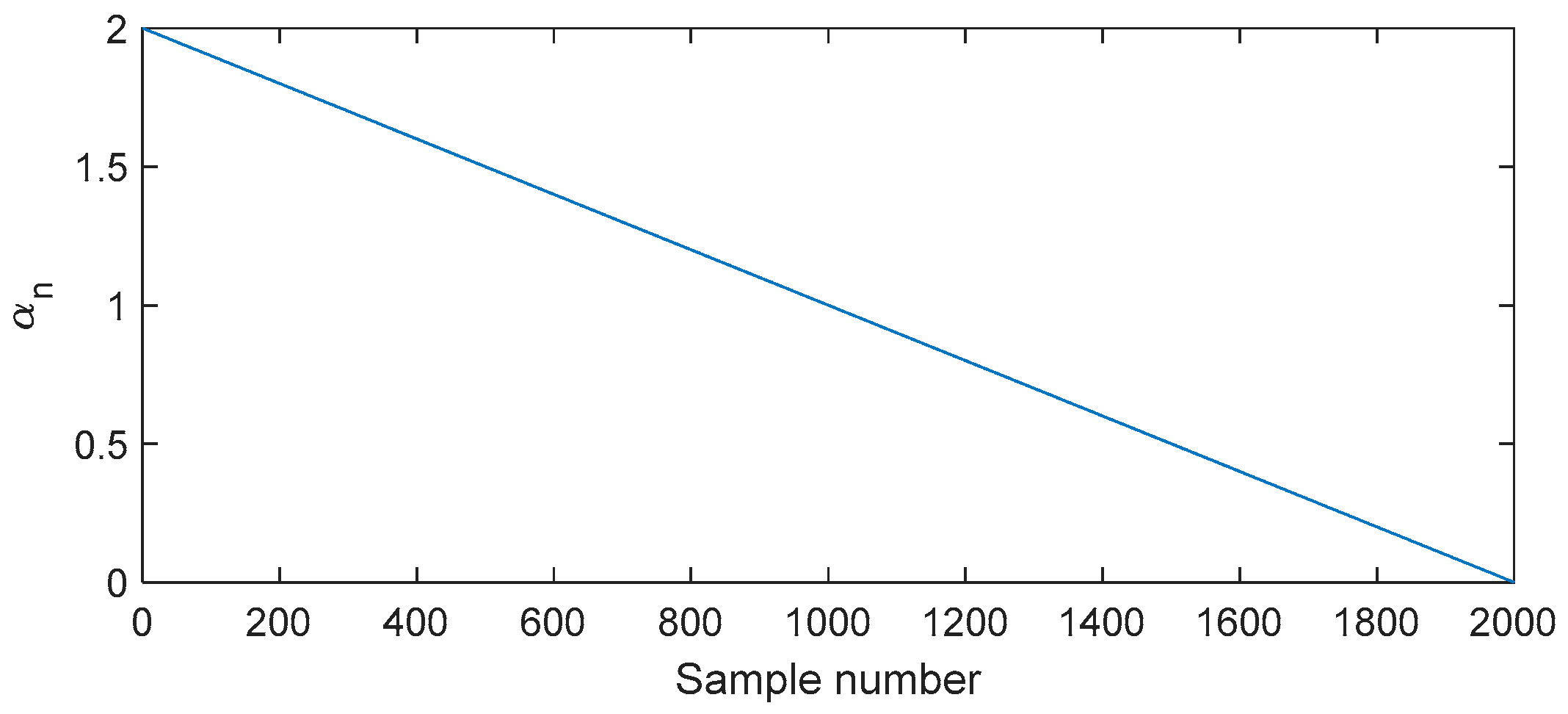
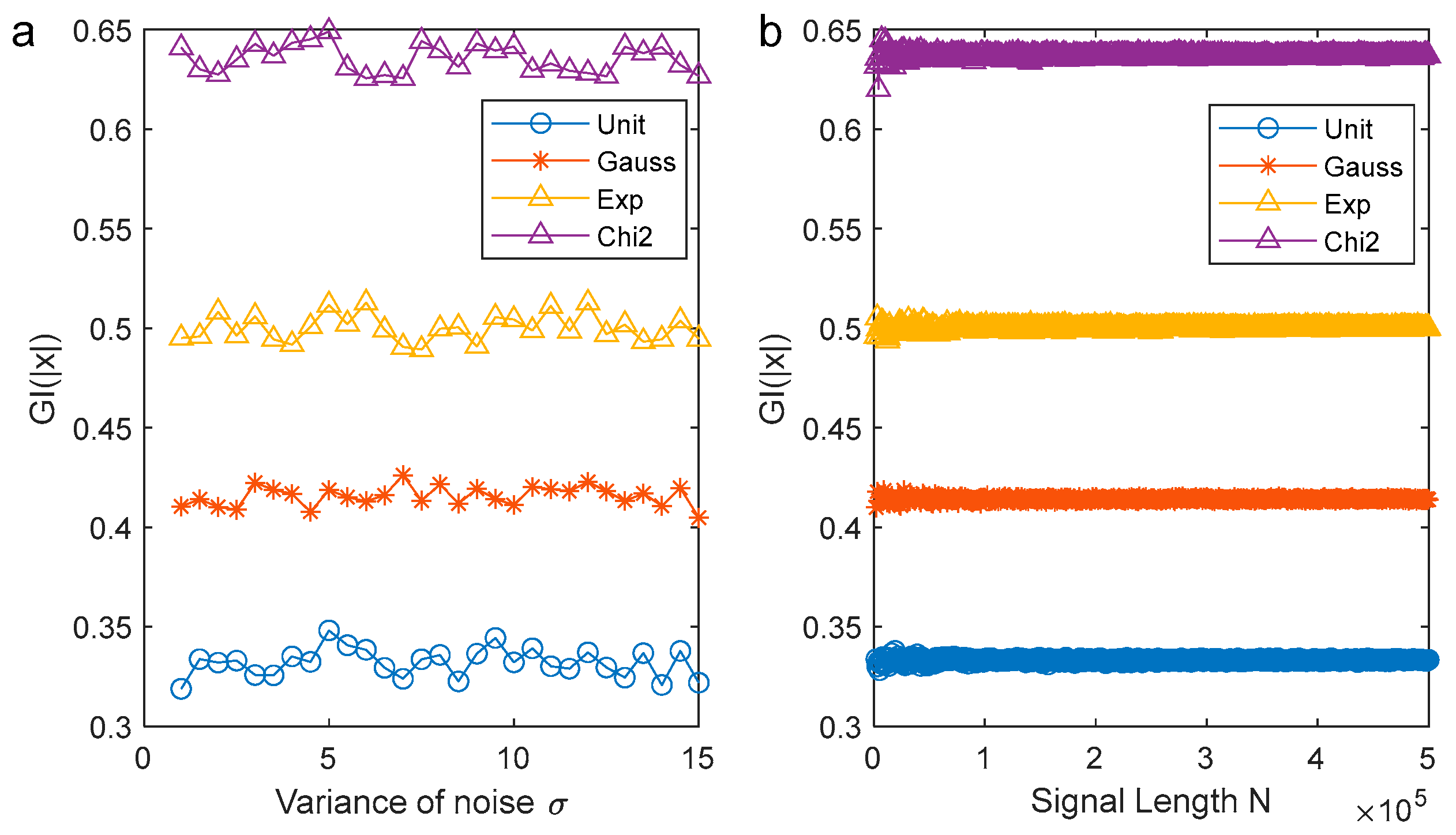
The series of cyclical impulses is one of most important signals in the fault diagnosis of rotating machines, because the impulses will be cyclically produced if a fault appears in the contact interfaces of REBs and gears.
Generally, an arbitrary series of ideal cyclical impulses with the amplitude of A can be denoted as
p n = A m = 1 M δ n m N M + 1 , n = 1 , , N , M = 1 ,   , N 1 ,          
where N denotes the length of the signal and M denotes the total number of cyclical impulses. δ n denotes the Dirac function. Obviously, there are M sample points whose value is A. Therefore, the series of order statistic is
p n = 0 , n = 1 , , N M A , n = N M + 1 , , N .                          
Then, the GI of the series of ideal cyclical impulse is
γ = 1 2 n = 1 N p n p 1 N n + 1 / 2 N = 1 2 × M 2 N = 1 M N   .                  
The derivation is shown in Appendix A.1. It can be seen that the GI value of the series of ideal cyclical impulses decreases with the increase in the total number of cyclical impulses when the length of the signal is fixed. If the total number of the cyclical impulses M is fixed, then the GI value of the series of ideal cyclical impulse increases with the increase in the length of signal. Apparently, M / N denotes the density of the cyclical impulses. It means that the smaller the density of cyclical impulses is, the bigger the GI value of the series of ideal cyclical impulses is. This result is consistent with the sparsity of the signal. Namely, the smaller the density of cyclical impulses, the sparser the series of ideal cyclic impulses is.

3.3. White Noise

In the engineering applications, noise is inevitable. Generally, the noise is white and can be denoted as a random series with a Gauss distribution of N μ , σ 2 .
Without loss of generality, white noise with a distribution of N 0 , σ 2 is considered and the series of absolute value w n , n = 1 , . . . , N is used, because the GI is defined on a series with the positive values. It is known that w n , n = 1 , . . . , N obeys the semi-normal distribution, whose probability density function (pdf) and cumulative distribution function (cdf) are given by [10]
f X w = 2 π σ 2 · e x p w 2 2 σ 2 u w , w R ,      
F X w = e r f w σ 2 u w ,                      
where u x denotes the unit step function whose formula is given by
u x = 1 , x 0 0 , x < 0   ,                          
and e r f x denotes the error function whose formulation is given by
e r f x 2 π 0 x e x p v 2 d v .                        
The average and variance of w n , n = 1 , . . . , N are given by
μ w = σ 2 / π     ,   σ w 2 = σ 2 π 2 π .                        
Because the expectation of the summation of a series equals the summation of the expectation of each random variable in the series, the following equation exists:
E n = 1 N w n = n = 1 N E w n = N σ 2 / π   .            
On the other hand, the order statistic series of w k , k = 1 , . . . , N can be denoted as w 1 < < w k < < w N , k = 1 , . . . , N . Suppose that the pdf and cdf of a random variable X are given by p x and F x ; then, the pdf of kth-order statistic X k is [10]
g y k = N ! k 1 ! N k ! F y k k 1 1 F y k n k p y k .          
Substituting Equations (7) and (8) into Equation (13), we can obtain the pdf of the kth-order statistic w k as follows:
g X w k = N ! k 1 ! N k ! F X w k k 1 1 F X w k N k f X w k = N ! k 1 ! N k ! e r f w σ 2 k 1 1 e r f w σ 2 N k 2 π σ 2 · e x p w k 2 2 σ 2 u w k   .
In this instance, the expectation of the kth-order statistic w k is
E X w k = w k g X w k d w k = 0 w k N ! k 1 ! N k ! e r f w k σ 2 k 1 1 e r f w k σ 2 N k 2 π σ 2 · e x p w k 2 2 σ 2 d w k = 2 π σ 2 N ! k 1 ! N k ! 0 w k e r f w k σ 2 k 1 · 1 e r f w k σ 2 N k · e x p w k 2 2 σ 2 d w k ,      
and the following equations exist.
E k = 1 N w k = 2 π σ 2 k = 1 N N ! k 1 ! N k ! 0 w k e r f w k σ 2 k 1 · 1 e r f w k σ 2 N k · e x p w k 2 2 σ 2 d w k ,
E k = 1 N α k w k = 2 π σ 2 k = 1 N α k · N ! k 1 ! N k ! 0 w k e r f w k σ 2 k 1 1 e r f w k σ 2 N k e x p w k 2 2 σ 2 d w k .
It can be seen that the accurate values of Equations (16) and (17) are based on the calculation of e r f x . Unfortunately, it is known to all that there is no closed expression for the cdf of Gauss distribution. Therefore, Equations (16) and (17) are also not closed. To address this question, the numerical methods are considered here. Figure 2 illustrates the numerical results of g X w k , w k g X w k and α k w k g X w k of the order statistic of the white noise when the length N equals 5. It can be seen that the values of g X w k , w k g X w k and α k w k g X w k are finite and decrease fast along the horizontal axis. Therefore, Equations (16) and (17) are finite and the expectations of order statistic variables and weighted order statistic variables exist.
Figure 3a illustrates the GIs of noises with different distributions, including the unit, Gauss, exponential and chi-square distributions. The variances of noises are changed from 1 to 15. It can be seen that there is only a little fluctuation for the GI values of different noises when the variance of the noise increases and the GI values of noises with different distributions are different from each other. In this case, we can deduce that E k = 1 N α k x k is proportional to k = 1 N E x k , although the integration in the expectation of kth-order statistic variable E X x k is not closed and we cannot write the explicit expressions of E X x k and E X k = 1 N x k . Figure 3b shows that the GI values of the noises with the distributions of unit, Gauss, exponent and chi-square vary with the length of noise. Similar to Figure 3a, it can be seen that there is also only a little fluctuation of GI values when the length N changes. By comparing Figure 3a,b, it can be deduced that the GI value of noise is mainly influenced by the distribution. Therefore, we suppose that
E k = 1 N α k w k = ρ N k = 1 N E w k .      
In this instance, the GI of the white noise can be calculated by
γ = 1 2 n = 1 N w n w 1 N n + 1 / 2 N = 1 n = 1 N α n w n n = 1 N w n , x n 0 ,    = 1 n = 1 N α n w n N σ 2 / π = 1 ρ N N σ 2 / π N σ 2 / π = 1 ρ N   .            
From Figure 3b, we can estimate that the GI of white noise with Gauss distribution is almost 0.4142 when the length N is closed to positive infinity. Therefore, the coefficient ρ N   e q u a l s   0.5858 for the white noise.

3.4. White Noise with Positive Bias

For the white noise with non-zero bias, it can be denoted by
x n = c + w n , n = 1 , . . . , N ,                                        
where c denotes the bias. Because the GI is based on the signal with positive value, we suppose that w n 0 , and c + w n = c + w n . In this case, the GI of the signal with non-zero bias is
γ = 1 2 n = 1 N x n x 1 N n + 1 / 2 N = 1 ρ N σ 2 / π + c σ 2 / π + c .        
The detailed derivation is listed in Appendix A.2. It can be seen that the GI value decreases with the increase in the bias c. For a fixed bias, the bigger the variance of the noise, the bigger the GI value. It means that the bias of a signal has an important influence on the calculation of the GI value and it is better to eliminate the bias before calculating the GI of a signal.

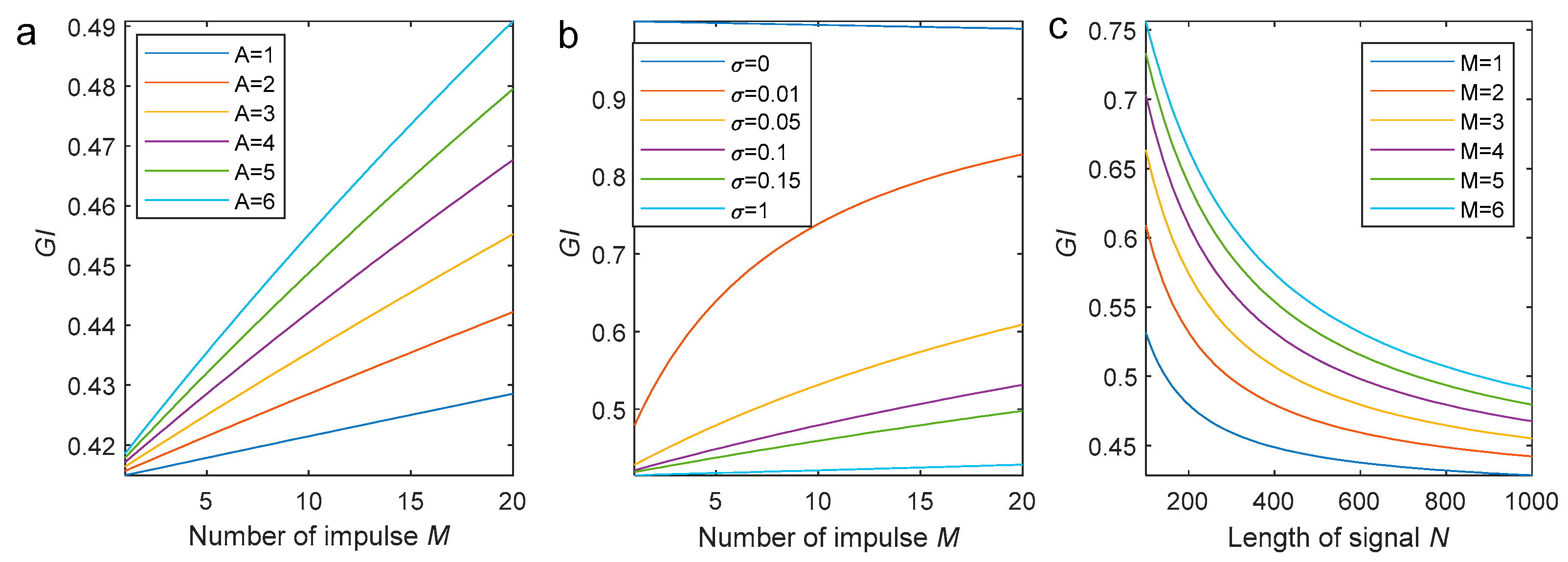
3.5. Cyclic Impulse Series with White Noise

In engineering applications, if there is a fault occurring on the contact interface of the REB and gear, the collected vibration is commonly the synthesis of the fault-induced vibration and the noise. Therefore, for the sake of calculation and understanding, the collected vibration is denoted by the summation of the cyclical impulse series and the white noise. Namely,
y n = A m = 1 M δ n m N M + 1 + w n , n = 1 , , N ,            
where A denotes the amplitude of the impulses, M denotes the total number of the impulses and w n ,   n = 1 , , N denotes the white noise with a distribution of N 0 , σ 2 . Then, the order statistic variable series of the collected vibration can be given by
y n = w n , n = 1 , , N M A + w n , n = N M + 1 , , N   .              
Suppose that the amplitude of the impulse A is bigger than the variance of the noise. Namely, A σ . Then, A + w n   A for arbitrary n. Then, we will obtain the GI of the cyclic impulse series with white noise by referring to Equation (19).
γ = 1 2 n = 1 N y n y 1 N n + 1 / 2 N = 1 n = 1 N M α n w n + M A M 2 N n = 1 N M w n + M A     = 1 ρ N N M σ 2 / π + M A M 2 N N M σ 2 / π + M A .                                            
The detailed derivation is listed in Appendix A.3.
Figure 4a illustrates the theoretical variation trends of the GI along the increase in the impulse number M when the signal length N equals 1000 and the variance of white noise σ equals 1. It can be seen that the GI of cyclic impulse series with white noise increases with the increment of the impulse numbers when the signal length is fixed. Moreover, the bigger the amplitude of the impulses, the bigger the GI value. Figure 4b illustrates the theoretical variation trends of the GI along the increase in the impulse number M when the signal length N equals 1000 and the amplitude of impulse A equals 20. The figure shows that the white noise plays an important role in the GI calculation of cyclic impulse series. When there is no noise, the GI deceases with the increase in the impulse number. This is consistent with the decrease in the sparsity of a signal. It means that the sparsity decreases because the energy of the cyclic impulse series is distributed to more impulses. However, when the white noise with small variance is added into the cyclic impulse series, the GI increases with the increment of the impulse number. Moreover, the bigger the signal-to-noise ratio (SNR), the bigger the GI value for a fixed number of impulses. Figure 4c shows the variation in the GI along the increase in signal length when the variance of white noise σ equals 1 and the amplitude of impulse A equals 20. It can be seen that the GI values decrease when the length of cyclic impulse series with added white noise increases. Because the amplitude of the impulse does not change, the growth of the signal length means the reduction of the SNR. Therefore, the GI of cyclic impulse series with white noise is comprehensively influenced by the amplitude of the impulse, the number of impulses and the degree of noise. This result has not been revealed in the previous literature because most of the existing literature does not consider the influence of noise despite noise being inevitable in engineering applications.

4. Numerical Simulations

In this section, two numerical simulations are performed to validate the correction of the proposed idea. The GIs of white noise with a Gauss distribution of N 0 , σ 2 with different biases added are calculated. The variances σ of the noises are set from one to six and the results are illustrated in Figure 5a. The GI of the numerical simulation is calculated when the length of the signal is 50,000 and is denoted by the scatter points. The solid lines denote the theoretical results of Equation (21). It can be seen that the simulation results coincide with the theoretical results very well and the GI values of white noises decrease with the growth of the positive bias. It means that the bias will affect the calculation of the signal GI.
On the other hand, a cyclic impulse series with an amplitude A of 1 is produced and the impulse number varies from 1 to 20. The cyclic impulse series is interrupted by different degrees of white noise. The variances of the white noises are set to be, in order, 0, 0.001, 0.005, 0.01, 0.1 and 1. The GI of the noise interrupting cyclic impulse series is calculated numerically. To eliminate the random interruption of the white noise, the calculation is repeatedly performed 100 times. The averaged values of the GI are illustrated as the discrete points in Figure 5b. The solid lines show the variation trends of the GI along the increase in the impulse number M when the variance of the white noise is different. It can be seen that the numerical simulation shares the same variation trends with the theoretical analysis, which are similar to those shown in Figure 4b. Moreover, the smaller the variance of the white noise, the closer both the values of the simulation and theoretical calculation are. This phenomenon comes from the fact that the supposition A σ is not satisfied when the variance of the white noise increases close to 1. This is because the amplitude of the impulse is also 1.

5. Applications

Although the GI value of the cyclic impulse series with noise is comprehensively affected by the amplitude of the impulse, the number of impulses and the degree of noise, it can be seen that the GI is positively related to the number of impulses when only low degrees of white noise exist in the signal. Therefore, it can be deduced that the maximization of the GI is inclined to extract as many impulses as possible in applications because the noise is inevitable. Comparatively, it has been proved that the maximization of kurtosis is inclined to extract a single impulse with huge amplitude [11]. In this case, a method based on the maximization of the GI is proposed and applied to a simulation and two experimental signals to illustrate the usage of the GI in application. The maximization of the GI is used to design an optimal Morlet filter and the parameters of the Morlet filter are optimized by the genetic algorithm (GA). Moreover, the maximization of kurtosis is also applied to illustrate the performance of the GI in the experimental data analysis. The detailed procedure of the method can be seen in Ref. [16].

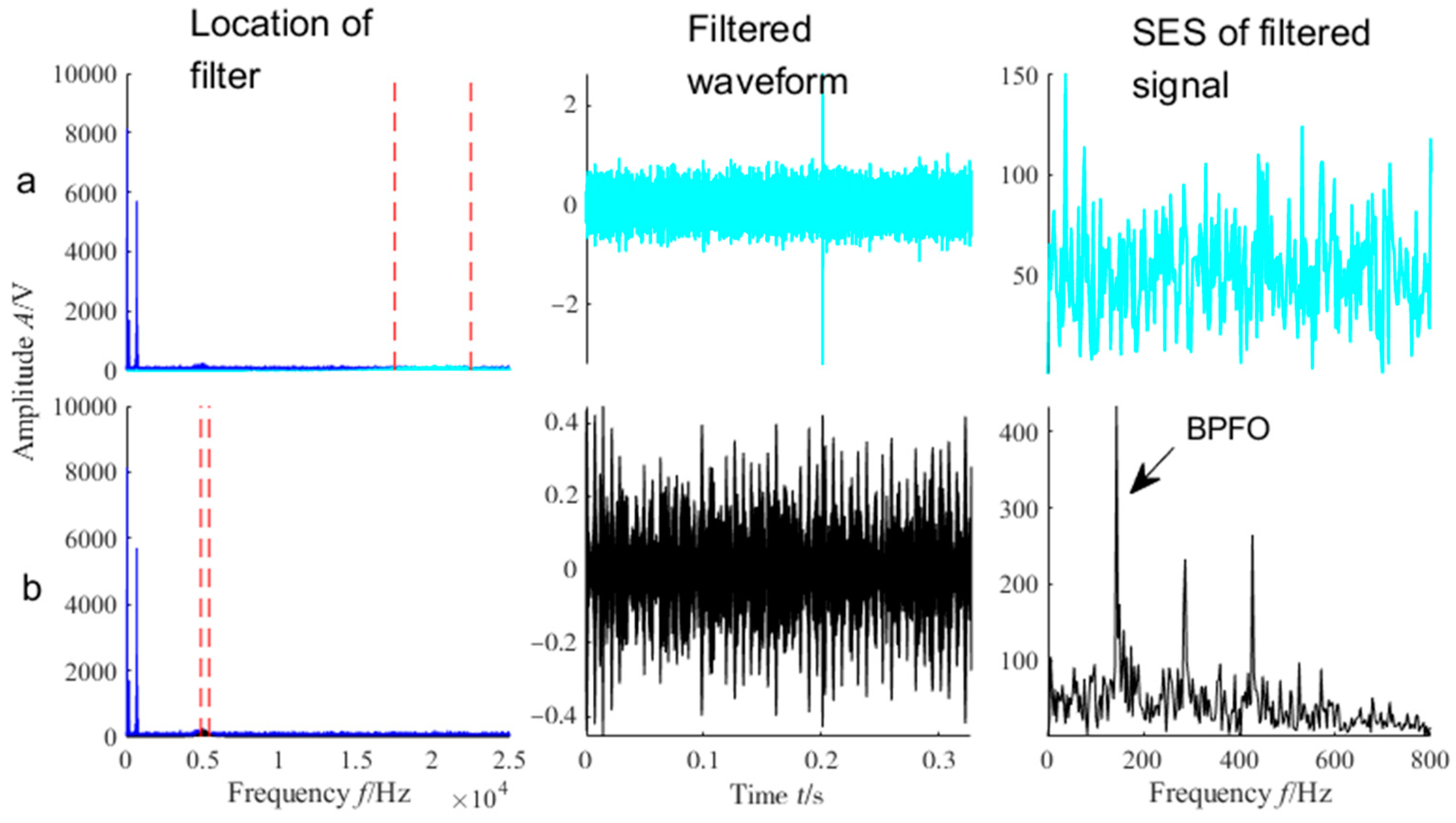
5.1. Simulation Analysis

REB fault diagnosis is used in the simulation analysis. The analytical model of the collected vibration caused by the bearing fault can be found in Ref. [16]. The detailed expression of the simulated signal is given by
y t = r t + g t + d t + p t h t ,            
where * denotes the convolution operator. r t denotes the forces caused by the shaft. g t denotes the force caused by the gear. d t denotes the external force. p t denotes the fault-induced impulsive force. h t denotes the unit impulsive response function of the bearing system. p t is usually given by
p t = a t k = 0 + δ t T k , T k + 1 = T k + T k   ,              
where a t denotes the amplitude of impulse force caused by the fault.   T k   denotes the occurrence moment of the kth impulse and T k denotes the temporal interval between the kth and (k + 1)th impulses. There is a little fluctuation in T k ,   k = 1,2 , because the rolling elements may experience some degrees of slippage on the races when the load is not uniform. Therefore, T k ,   k = 1,2 , is an independent increment process. h t is usually given by
h t = e x p ζ 2 π f n t · s i n 2 π f n t ,                  
where f n denotes the natural frequency and ζ denotes the damping ratio. In the simulation, suppose that the outer ring is fixed and the rotating frequency of the inner ring, denoted by f r , is 40 Hz. The natural frequency f n = 5   k H z , the damping ratio ζ = 0.04   and the ball pass frequency on the outer race (BPFO) equal 3.57 times the rotating frequency. Namely, B P F O = 3.57 × f r . Let a t = 10 ; the force caused by the shaft, gear and external force in the inner race fault simulation are given by
r ( t ) = 10 c o s ( 2 π f r t ) ,                                  
    g ( t ) = 4 1 + 0.5 cos 2 π f r t · cos ( 34 π f r t + cos 2 π f r t ) ,    
d ( t ) = 3 c o s ( 400 π t ) .                      
The fluctuation in the impulse interval is 0.3%. A pre-amplifier of 80 dB is used and the vibration is collected with the length of 8192 samplings by a frequency of 50 kHz. Furthermore, a white noise of 2 dB is added into the simulated vibration. Two outliers with a value of 10 are randomly added into the signal. For the sake of reducing the length of this paper, the waveform of the signal is neglected here and the spectrum can be seen in Figure 6.
Figure 6 illustrates the simulation analysis results obtained by using the methods of maximization of both kurtosis and the GI. The carrier frequency of the impulse response is 5 kHz and the simulation is affected by several random outliers. It can be seen that the outlier with large amplitude is extracted in the time domain by the method of maximizing the kurtosis and no fault feature can be noticed in the squared envelope spectrum (SES). Comparatively, many more cyclical impulses are extracted by the method of maximizing the GI and the first three orders of BPFO are visible in the SES. Namely, the maximization of the GI is inclined to extract more impulses than that of kurtosis in the same simulation.

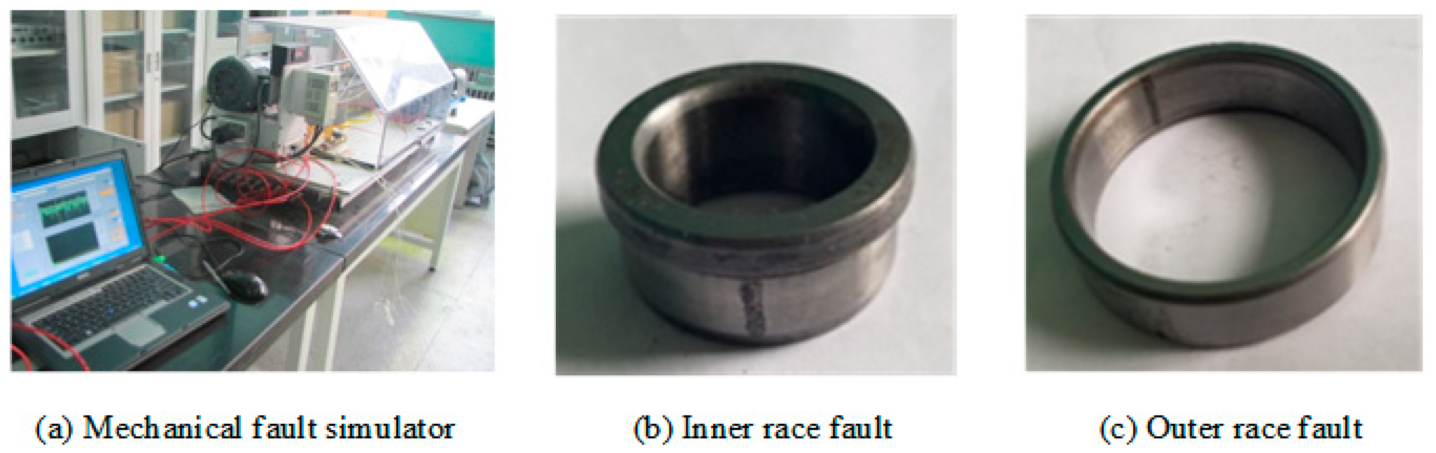
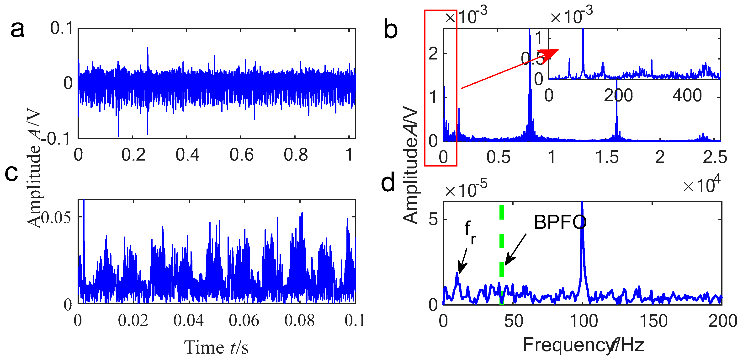
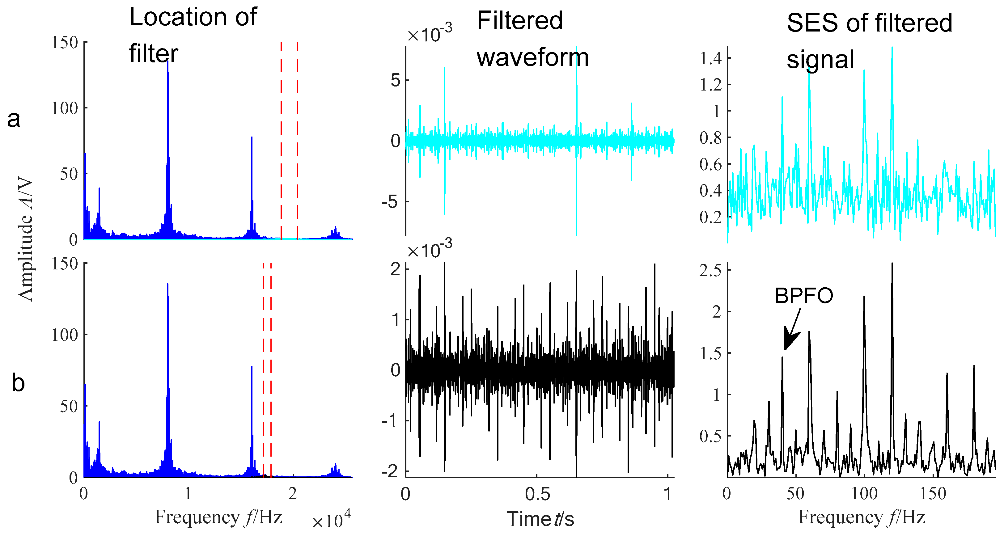
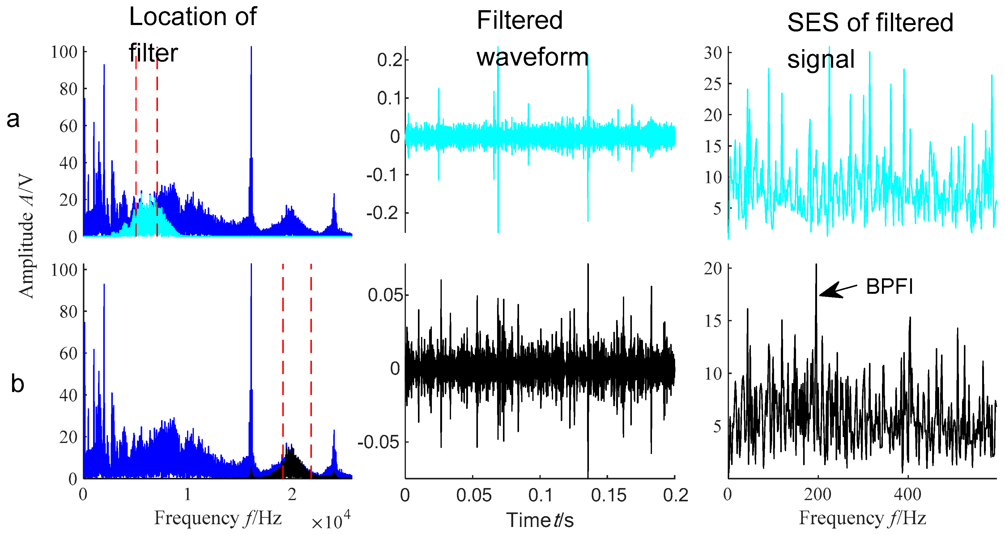
5.2. Experimental Analysis

The methods of maximizing both the kurtosis and GI are applied to two experimental signals in this section. The experiment was performed on the mechanical fault simulator in the laboratory of fault diagnosis at Tsinghua University. As shown in Figure 7, the rotor system is driven by an inverter motor though a coupling. A disk with a quality eccentricity of 10 g and a distance of 50 mm is mounted at the middle of the shaft. Two loading disks of 5 kg are symmetrically installed on both sides of the middle disk. The whole test rig is supported by eight rubber bases. The shaft is supported by two rolling element bearings (REBs) of NSK NJ 6204EM, manufacutred by NSK, Shanghai, China. The diameter of the outer race is 47 mm, the diameter of the inner race is 20 mm and the pitch diameter is 33.5 mm. There are 11 rolling elements in the bearing and the diameter of the rolling element is 13.5 mm. The outer race fault and inner race fault with a circumferential width of 1 mm are manually added by an electric discharge machine (EDM). In this instance, the BPFO and BPFI equal 4.295 and 6.561 times the rotating frequency, respectively. The faulty bearing is mounted at the drive end of the shaft and a Dytran 3650C piezoelectric acceleration sensor is vertically mounted on the bearing house. The data are acquired by 34970A Agilent data acquisition equipment. All vibration signals are sampled by the frequency of 51.2 kHz and have a length of 10.2 s.
Figure 8 displays the waveform, spectrum, raw envelope and SES of the outer race fault test signal when the rotating frequency of the shaft is 9.766 Hz. It can be seen that several impulses/outliers exist in the waveform. Only two discrete lines are located at the rotating frequency of 9.766 Hz and 100 Hz in the SES. No fault feature can be noticed in both the spectrum and SES.
Figure 9 displays the experimental analysis result of the outer race fault obtained by the method of maximizing both the kurtosis and GI when the rotating frequency of the shaft is 9.766 Hz. The convergence processes of both GAs are sequentially terminated at the 57th and 100th generation. It can be seen that several outliers are visible in the filtered waveform obtained by the method of maximizing the kurtosis. Comparatively, many more cyclical impulses are extracted by the method of maximizing the GI and the first two orders of BPFO are visible in the SES. Moreover, the SES of the filtered signal obtained by the method of maximizing the GI is more concise than that obtained by the method of maximizing the kurtosis.
Figure 10 shows the waveform, spectrum, raw envelope and SES of the inner race fault test signal when the rotating frequency is 59.67 Hz. An impulse/outlier exists in the waveform. Only a weak discrete spectral line located at the frequency of 2 × B P F I and no other fault features can be noticed.
Figure 11 displays the experimental analysis result of the inner race fault obtained by the method of maximizing both the kurtosis and GI when the rotating frequency is 29.8 Hz. The convergence processes of both GAs are terminated at the 100th generation. It can be seen that several outliers are visible in the filtered waveform obtained by the method of maximizing the kurtosis. Comparatively, many more cyclic impulses are extracted by the method of maximizing the GI and the BPFI and are visible in the SES.

6. Conclusions

As a commonly used sparsity characterizing index of the signal, the GI has been introduced into the fault diagnosis of rotating machines. However, why the GI can be used for representing the impulse characteristic of the signal has not been considered yet. In this case, the mathematical mechanism of the GI used for the representation of the multiple-impulse phenomenon was deeply researched based on the theoretical derivation of the GIs of several typical signals. Numerical simulations were performed to validate the correction of the derivation. The following results and conclusions can be obtained.
(1)
The GI of the constant signal is zero. If there is a large bias in the signal, the bias should be canceled first before the calculation of the GI.
(2)
The GI of the ideal cyclical impulse series decreases with the increase in the impulse number.
(3)
The distribution of the noise plays an important role in the calculation of the GI. The GI of white noise with normal distribution is around 0.4142.
(4)
For the cyclic impulse series affected by white noise, the GI is influenced in a comprehensive manner by the amplitude of the impulse, the number of impulses and the degree of noise. Generally, the GI increases with the increment of the impulse number. The bigger the difference between the amplitude of the impulse and the variance of the white noise, the greater the value of GI is. Therefore, the GI is powerful when it is used for characterizing the impulsive intensity of the multiple-impulse phenomenon.
(5)
Both simulation and experimental analyses show that methods based on the maximization of the GI can be used for the extraction of cyclical impulses and are more powerful than those based on the maximization of kurtosis.

Author Contributions

Conceptualization, A.M. and W.Z.; methodology, A.M.; validation, G.J.; formal analysis, G.J. investigation, G.J.; writing—original draft preparation, G.J.; writing—review and editing, W.Z.; visualization, A.M.; funding acquisition, A.M. and W.Z. All authors have read and agreed to the published version of the manuscript.

Funding

This work was partly supported by the Research Start-up Project of Northwestern Polytechnical University under Grant No. G2021KY05104, the Natural Science Foundation of Shaanxi Province under Grant No. 2023-JC-YB-436 and the National Natural Science Foundation of China under Grant No. 52475134.

Data Availability Statement

The raw data supporting the conclusions of this article will be made available by the authors on request.

Acknowledgments

All authors greatly appreciate the help of Fulei Chu at Tsinghua University during the research.

Conflicts of Interest

The authors declare no conflicts of interest. The funders had no role in the design of the study; in the collection, analyses or interpretation of data; in the writing of the manuscript; or in the decision to publish the results.

Appendix A

Appendix A.1. Derivation of Equation (6)

For the ideal impulse series, the GI is
                                                      γ = 1 2 n = 1 N p n p 1 N n + 1 / 2 N .                                
Because part of the ideal impulse series is zero, by referring Equation (5), we can obtain the following equation.
γ = 1 2 n = 1 N M 0 M A N n + 1 / 2 N + n = N M + 1 N A M A N n + 1 / 2 N                     = 1 2 M N N M + 1 + 1 / 2 N + 1 / 2 N M 2 = 1 M N .                                              

Appendix A.2. Derivation of Equation (21)

For the white noise with positive bias, the GI is
= 1 2 n = 1 N x n x 1 N n + 1 / 2 N = 1 n = 1 N α n x n n = 1 N x n , x n 0   .          
If we substitute Equation (20) into Equation (A3), then following equations exist:
  γ = 1 n = 1 N α n c + w n n = 1 N c + w n = 1 n = 1 N α n w n + n = 1 N α n c n = 1 N w n + n = 1 N c                                                                                                     = 1 ρ N N σ 2 / π + N c N σ 2 / π + N c   = 1 ρ N σ 2 / π + c σ 2 / π + c .                                                                            

Appendix A.3. Derivation of Equation (24)

For the cyclic impulse series with white noise of N 0 , σ 2 , the GI is
γ = 1 2 n = 1 N y n y 1 N n + 1 / 2 N = 1 2 n = 1 N y n y 1 N n + 1 / 2 N                                                   = 1 2 n = 1 N y n N n + 1 / 2 N y 1 = 1 2 n = 1 N y n N n + 1 / 2 N n = 1 N y n .                      
If we substitute Equation (23) into Equation (A5), then we will obtain
γ = 1 2 n = 1 N M w n N n + 1 / 2 N + n = N M + 1 N A + w n N n + 1 / 2 N n = 1 N M w n + n = N M + 1 N A + w n .        
Because A σ , therefore, A + w n   A for arbitrary n. Then, we will obtain the following equations.
γ = 1 2 n = 1 N M w n N n + 1 / 2 N + n = N M + 1 N A N n + 1 / 2 N n = 1 N M w n + n = N M + 1 N A    = 1 2 n = 1 N M w n N n + 1 / 2 N + A N N M + 1 + 1 / 2 N + 1 / 2 N M 2 n = 1 N w n + N M A = 1 2 n = 1 N M w n N n + 1 / 2 N + A M 1 / 2 N + 1 / 2 N M 2 n = 1 N w n + M A   = 1 2 n = 1 N M w n N n + 1 / 2 N + A M N M 2 n = 1 N w n + M A     = 1 2 n = 1 N M w n N n + 1 / 2 N + M A M 2 N n = 1 N M w n + M A = 1 n = 1 N M α n w n + M A M 2 N n = 1 N M w n + M A       = 1 ρ N N M σ 2 / π + M A M 2 N N M σ 2 / π + M A .
From Equation (A7), it can be seen that the GI of the cyclic impulse series with noise is affected in a comprehensive manner by the amplitude of the impulse, the number of impulses and the degree of noise.

References

  1. Molero-Simarro, R. Inequality in China revisited. The effect of functional distribution of income on urban top incomes, the urban-rural gap and the Gini index, 1978–2015. China Econ. Rev. 2017, 42, 101–117. [Google Scholar] [CrossRef]
  2. Miao, Y.; Zhao, M.; Lin, J. Improvement of kurtosis-guided-grams via Gini index for bearing fault feature identification. Meas. Sci. Technol. 2017, 28, 125001. [Google Scholar] [CrossRef]
  3. Miao, Y.; Wang, J.; Zhang, B.; Li, H. Practical framework of Gini index in the application of machinery fault feature extraction. Mech. Syst. Signal Process. 2022, 165, 108333. [Google Scholar] [CrossRef]
  4. Antoni, J. Fast computation of the Kurtogram for the detection of transient faults. Mech. Syst. Signal Process. 2007, 21, 108–124. [Google Scholar] [CrossRef]
  5. Barszcz, T.; Jablonski, A. A novel method for the optimal band selection for vibration signal demodulation and comparison with the Kurtogram. Mech. Syst. Signal Process. 2011, 25, 431–451. [Google Scholar] [CrossRef]
  6. Wang, T.; Han, Q.; Chu, F.; Feng, Z. A new SKRgram based demodulation technique for planet bearing fault detection. J. Sound Vib. 2016, 385, 330–349. [Google Scholar] [CrossRef]
  7. Nassef, M.G.A.; Hussein, T.M.; Mokhiamar, O. An adaptive variational mode decomposition based on sailfish optimization algorithm and Gini index for fault identification in rolling bearings. Measurement 2021, 173, 108514. [Google Scholar] [CrossRef]
  8. Hou, B.; Wang, D.; Xia, T.; Xi, L.; Peng, Z.; Tsui, K.-L. Generalized Gini indices: Complementary sparsity measures to Box-Cox sparsity measures for machine condition monitoring. Mech. Syst. Signal Process. 2022, 169, 108751. [Google Scholar] [CrossRef]
  9. Chen, B.; Cheng, Y.; Zhang, W.; Gu, F. Investigations on improved Gini indices for bearing fault feature characterization and condition monitoring. Mech. Syst. Signal Process. 2022, 176, 109165. [Google Scholar] [CrossRef]
  10. Wang, D. Some further thoughts about spectral kurtosis, spectral L2/L1 norm, spectral smoothness index and spectral Gini index for characterizing repetitive transients. Mech. Syst. Signal Process. 2018, 108, 360–368. [Google Scholar] [CrossRef]
  11. Shynk, J.J. Probalility, Random Variables, and Random Processes Theory and Signal Processing Applications; Willey: Hoboken, NY, USA, 2012. [Google Scholar]
  12. Miao, Y.; Zhao, M.; Hua, J. Research on sparsity indexes for fault diagnosis of rotating machinery. Measurement 2020, 158, 107733. [Google Scholar] [CrossRef]
  13. Tong, S.; Fu, Z.; Tong, Z.; Cong, F. Gear fault diagnosis using spectral Gini index and segmented energy spectrum. Meas. Sci. Technol. 2024, 35, 116134. [Google Scholar] [CrossRef]
  14. Yu, Y.; Zhao, X. Separation of fault characteristic impulses of flexible thin-wall bearing based on wavelet transform and correlated Gini index. Mech. Syst. Signal Process. 2024, 209, 111118. [Google Scholar] [CrossRef]
  15. Chen, B.; Song, D.; Cheng, Y.; Huang, B.; Muhamedsalih, Y. IGIgram: An Improved Gini Index-Based Envelope Analysis for Rolling Bearing Fault Diagnosis. J. Dynamics. Monit. Diagn. 2022, 1, 111–124. [Google Scholar] [CrossRef]
  16. Ming, A.; Zhang, W.; Fu, C.; Yang, Y. L-kurtosis-based optimal wavelet filtering and its application to fault diagnosis of rolling element bearings. J. Vib. Control. 2024, 30, 1594–1603. [Google Scholar] [CrossRef]
Figure 1. αn of the GI when the length of the series N equals 2000.
Aerospace 11 01034 g001
Figure 2. g X w k , w k g X w k and α k w k g X w k of the order statistic of the white noise.
Aerospace 11 01034 g002
Figure 3. GI values of noises with different distributions and different signal lengths. (a) Influence of the variance of noise; (b) influence of the signal length.
Aerospace 11 01034 g003
Figure 4. Theoretical GI of the cyclic impulse series with noise at different conditions. (a) GI values of cyclic impulse series with different numbers of impulses; (b) GI values of cyclic impulse series with different degrees of noise; (c) GI values of cyclic impulse series with different signal lengths.
Aerospace 11 01034 g004
Figure 5. Comparison of the theoretical and simulation results.
Aerospace 11 01034 g005
Figure 6. Simulation analysis results: (a) location of filter, filtered waveform and SES of filtered signal obtained by the method of maximizing the kurtosis; (b) location of filter, filtered waveform and SES of filtered signal obtained by the method of maximizing the GI (The blue lines represent the spectrum of the signal. The red dashed lines represent the lower and upper bounds of the filter.).
Aerospace 11 01034 g006
Figure 7. Experimental equipment and bearing faults.
Aerospace 11 01034 g007
Figure 8. Waveform (a), spectrum (b), raw envelope (c) and SES (d) of outer race fault test signal (The green dashed line denotes the locations of the harmonics of BPFO. The red square denotes the zooming out area of the spectrum.).
Aerospace 11 01034 g008
Figure 9. Experimental analysis result of outer race fault: (a) location of filter, filtered waveform and SES of filtered signal obtained by the method of maximizing the kurtosis; (b) location of filter, filtered waveform and SES of filtered signal obtained by the method of maximizing the GI (The blue lines represent the spectrum of the signal. The red dashed lines represent the lower and upper bounds of the filter.).
Aerospace 11 01034 g009
Figure 10. Waveform (a), spectrum (b), raw envelope (c) and SES (d) of inner race fault test signal.
Aerospace 11 01034 g010
Figure 11. Experimental analysis result of inner race fault: (a) location of filter, filtered waveform and SES of filtered signal obtained by the method of maximizing the kurtosis; (b) location of filter, filtered waveform and SES of filtered signal obtained by the method of maximizing the GI (The blue lines represent the spectrum of the signal. The red dashed lines represent the lower and upper bounds of the filter.).
Aerospace 11 01034 g011
Disclaimer/Publisher’s Note: The statements, opinions and data contained in all publications are solely those of the individual author(s) and contributor(s) and not of MDPI and/or the editor(s). MDPI and/or the editor(s) disclaim responsibility for any injury to people or property resulting from any ideas, methods, instructions or products referred to in the content.

