Article

A Data-Driven Feature Extraction Process of Interleaved DC/DC Converter Due to the Degradation of the Capacitor in the Aircraft Electrical System

School of Automation, Northwestern Polytechnical University, Xi’an 710072, China
*
Author to whom correspondence should be addressed.
Aerospace 2024, 11(12), 1027; https://doi.org/10.3390/aerospace11121027
Submission received: 23 October 2024 / Revised: 8 December 2024 / Accepted: 13 December 2024 / Published: 16 December 2024
(This article belongs to the Special Issue Aircraft Electric Power System: Design, Control, and Maintenance)

Abstract

:
In recent years, preventive maintenance has emerged as a focal point of research in the aerospace field. The concept of equipment maintenance, exemplified by prognosis and health management (PHM), has permeated every aspect of development and design. Extracting degradation features presents a fundamental and challenging task for health assessment and remaining useful life prediction. To facilitate the efficient operation of the incipient fault diagnosis model, this paper proposes a data-driven feature extraction process for converters, which consists of two main stages. First, feature extraction and comparison are conducted in the time domain, frequency domain, and time–frequency domain. By employing wavelet decomposition and the Hilbert transform method, a highly correlated time–frequency domain feature is obtained. Second, an improved feature selection approach that combines the ReliefF algorithm with the correlation coefficient is proposed to effectively minimize redundancy within the feature subset. Furthermore, an incipient fault diagnosis model is established using neural networks, which verifies the effectiveness of the data-driven feature extraction process presented herein. Experimental results indicate that this method not only maintains fault diagnosis accuracy but also significantly reduces training time.

1. Introduction

With the evolution of aircraft towards more and all-electric systems, DC/DC converters are playing an increasingly crucial role in the aviation field. These converters are responsible for converting DC power from one voltage level to another to meet the varying voltage requirements of different electronic devices [1]. As the power ratings continue to increase, aircraft may encounter diverse environmental disturbances and electromagnetic interferences, necessitating that the DC/DC converter provide a stable voltage supply to ensure the safe operation of the load. The primary factors affecting the performance of the DC/DC converter include temperature, electrical stress, and aging [2]. Failure or malfunction of the converter can result in improper functioning of electronic devices and may even lead to a complete system collapse. Consequently, the reliability of DC/DC converters is vital for system safety.
DC/DC converter failures can be categorized into two types based on their characteristics and behavior: hard failures and soft failures [3,4]. Hard failures result in catastrophic outcomes, often due to significant component damage within the circuit, such as short circuits or open circuits. In contrast, soft failures generally do not lead to severe system damage and can be further subdivided into temporary failures and incipient failures. Temporary failures typically involve brief voltage fluctuations and circuit anomalies, which may cause transient variations in system performance. These failures are frequently attributed to environmental changes or fluctuations in input voltage. Incipient failures, also known as progressive failures, are primarily caused by the degradation (aging) of key components in the circuit. As the aviation industry has gradually shifted from periodic maintenance to condition-based maintenance (CBM) [5], novel technical concepts have emerged in recent years. Among these concepts, prognosis and health management (PHM) has garnered significant attention, emerging as a critical field of research in the current Industrial 4.0 revolution [6]. PHM utilizes condition monitoring data and information provided by operational practitioners to assess system health, detect potential anomalies, diagnose incoming faults, and predict the remaining useful life (RUL) [7]. Under the PHM framework, the diagnosis and evaluation of incipient failures have become a prominent research focus. The first step in these diagnostic or evaluation algorithms is feature extraction.
Feature extraction refers to the process of deriving useful information from raw data for classification and prediction. This process can eliminate redundant information and noise within the raw data, thereby enhancing the efficiency and quality of data processing [8]. The operating parameters of the circuit can be categorized into three types based on the signal form: time domain features, frequency domain features, and time–frequency domain features. Time domain features are currently the subject of extensive research due to their strong interpretability, as they encompass clear physical meanings. Commonly utilized time domain features include maximum and minimum value, mean value [9], variance [10], and root mean square [11]. B. R. Nayana and P. Geethanjali proposed 18 time–domain features for the early diagnosis of bearing faults [12], which consist of 6 time-dependent spectral features (TDSFs) and 12 statistical time domain features. This approach effectively captures the fault characteristics of mechanical structures such as bearings. These parameters, which possess units, are referred to as dimensioned metrics and are highly sensitive to environmental variables (e.g., load). Consequently, several dimensionless indicators, including kurtosis, skewness [13], waveform factor, peak factor, pulse factor, and margin factor, are employed to characterize degradation or early failures. In a study conducted by Sandeep and Sanjay [14], spectral kurtosis (SK) was adopted for the fault classification of rotating machines. A similar approach was employed by Tian et al. [15] to detect faults in motor bearings. Some features may not be adequately represented in the time domain; therefore, frequency domain analysis may be necessary. The Fast Fourier Transform (FFT) enables the transformation of time domain signals into the frequency domain, thereby providing a clearer representation of the signal’s properties and characteristics. Commonly used frequency domain indicators include characteristic frequency [16,17], mean square frequency [18], harmonics [19], frequency variance [20], etc. For instance, the study by Indrayudh et al. [21] incorporated both time domain features and frequency domain parameters, such as frequency center (FC), RMS variance frequency, and root variance frequency, significantly enhancing the representativeness of the features. Wang [22] also integrated both time domain and frequency domain features in the fault diagnostics of rolling bearings. Jing Yang [23] noted that time domain features do not effectively distinguish fault stages, while frequency domain features demonstrate superior performance in diagnosing the incipient fault of deep groove ball bearings. Through detailed frequency domain analysis, researchers have discovered that the harmonic components of certain signals are not fixed, and the patterns of these harmonics can also serve as features. In the early stages of a fault, the fault characteristics may present as a time-varying frequency component. Consequently, time–frequency domain features are gaining attention in the engineering field, as they can elucidate the trend of frequency changes in specific signals over time. In the study by Qiyue Li et al. [24], wavelet transform was employed to extract features in the time–frequency domain, yielding satisfactory results in the detection of incipient faults in power distribution systems. Fujin Deng et al. [25] proposed a feature extraction algorithm based on sliding time windows for fault localization in multilevel converters. This approach is conceptually similar to the wavelet transform and can be classified as a time–frequency domain feature extraction method.
In aerospace applications, extracting degradation features from converters presents numerous significant challenges and constraints. Firstly, to maintain system integrity and minimize interference, the feature extraction process must adopt non-intrusive methods whenever possible. This necessitates conducting the process without substantially increasing the burden on additional acquisition circuits, which would inevitably add complexity to technical implementation. In order to monitor the performance degradation of aircraft engines in real-time, Dasheng Xiao et al. [26] extracted 12 features, including environmental parameters, state parameters, and performance parameters, in a laboratory environment for screening. Concurrently, Umar Saleem et al. [27] developed a machine learning system for aircraft generator fault classification tasks, which performed wavelet decomposition on the three-phase output current of the generator to extract the standard deviations and means of all detail coefficients. Additionally, Yu Zhang et al. [28] conducted research on the degradation of aircraft auxiliary power units based on existing sensors, extracting data from five sensors, including start-up time and peak exhaust temperature. These studies illustrate the numerous limitations present in the measurement conditions for degradation research in aviation scenarios.
Based on the current research status, it is evident that there are three significant limitations in the field of feature extraction. The first limitation is the lack of a comparative analysis of features across the time domain, frequency domain, and time–frequency domain, which results in selected features being less robust and prone to information loss. The second limitation is that the majority of research has concentrated on the feature extraction of hard faults, such as short or open circuits, while there is limited exploration of soft fault features, such as aging. Finally, the correlation between features is often overlooked, which frequently leads to the inclusion of highly correlated or redundant features within the feature subset.
In response to the aforementioned issues, the innovative contributions of this paper are summarized as follows.
(1) This study concentrates on incipient failures of DC/DC converters, a process characterized by its slow progression and poorly differentiated features. Most incipient failures stem from aging and do not lead to significant changes in external characteristics, unlike hard failures. Nevertheless, identifying incipient faults is crucial for enhancing system reliability.
(2) The feature extraction presented in this paper is conducted across time, frequency, and time–frequency domains. Currently, few researchers have simultaneously performed feature extraction in all three domains within the field of power electronics. Additionally, a novel feature based on the time–frequency domain is proposed, which is highly relevant to the degradation process.
(3) An improved ReliefF algorithm is introduced in this paper to eliminate highly correlated features from the feature subset by integrating the Pearson correlation coefficient. This proposed feature selection method yields a more concise subset, which can significantly expedite the model’s training process.
The overall structure of the study is organized into five sections, including this introductory section. Section 2 presents the feature extraction methods relevant to each domain, with a particular emphasis on the time–frequency domain feature extraction method. Additionally, this section introduces the proposed ReliefF–Pearson-based feature selection method. Section 3 describes the experimental platform and the simulation of the degradation process. In Section 4, the feature extraction processes and results across the time, frequency, and time–frequency domains are detailed, along with the feature selection results and performance evaluations. Finally, Section 5 provides a summary of the entire paper.

2. Feature Extraction and Selection Methods

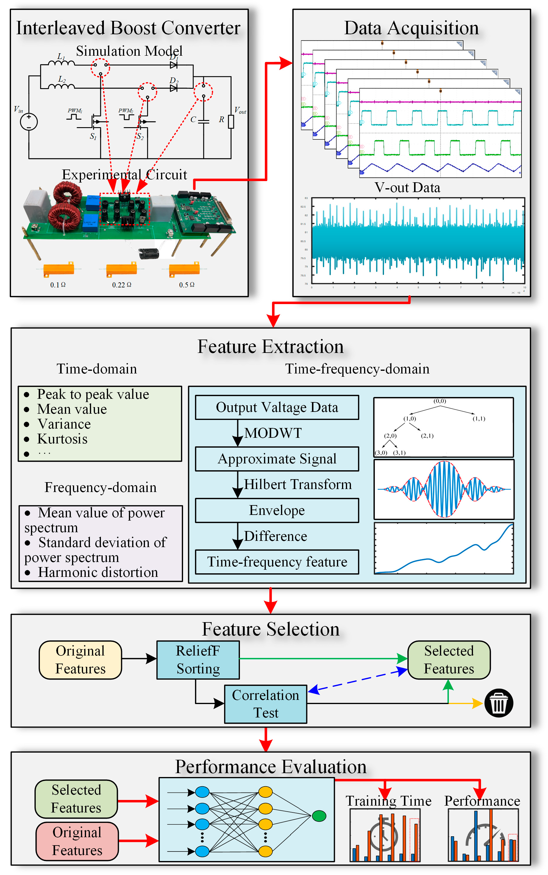
Feature extraction is fundamental to the implementation of PHM. The use of appropriate external features can significantly enhance the efficiency of fault diagnosis and prediction algorithms while also reducing the computational load. Time domain and frequency domain features are commonly employed to analyze signals from various perspectives. In this paper, five statistical indicators (such as mean value and variance) and three dimensionless parameters (including kurtosis) are extracted as time domain features. Frequency domain feature extraction is conducted through power spectrum analysis, wherein the mean value, standard deviation of the power spectrum, and the harmonic content are extracted. Currently, there is no standardized method for the extraction of time–frequency domain features, which necessitates a specific analysis tailored to the working scenario. Consequently, this paper proposes a method that integrates wavelet decomposition and the Hilbert transform to extract time–frequency domain features. The research flow of this paper is illustrated in Figure 1.
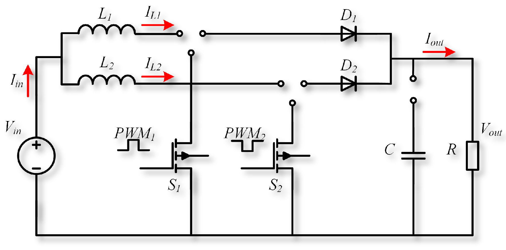
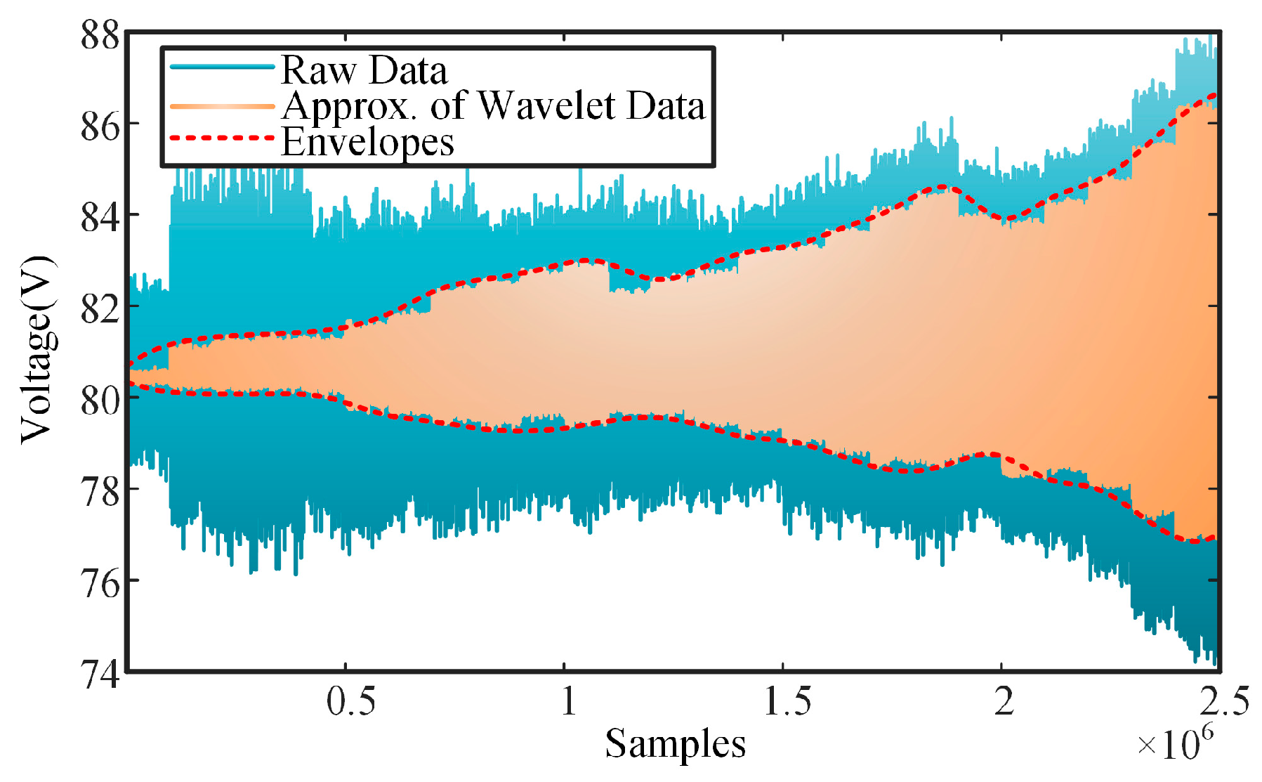
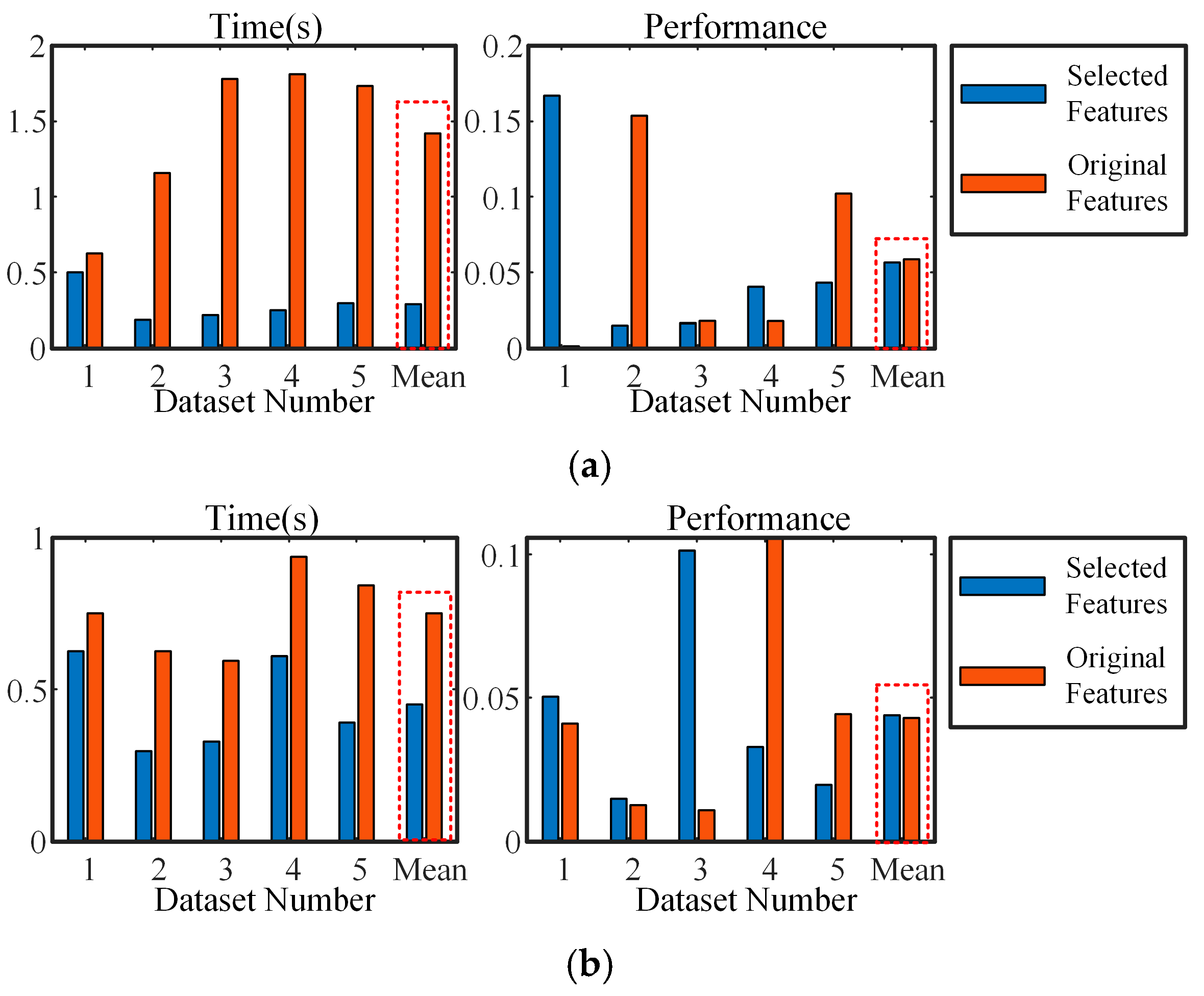
A practical interleaved boost converter serves as the experimental platform for this study. The output voltage is recorded as raw data by simulating the degradation process of the converter. Subsequently, features are extracted from three distinct domains. The proposed time–frequency domain feature extraction method processes the raw data by obtaining an approximate signal through wavelet decomposition. The Hilbert transform is then applied to derive the envelope of the approximate signal, with the difference between the upper and lower envelopes utilized as the time-frequency domain feature. During the feature selection phase, an improved ReliefF algorithm is introduced to rank the feature set and eliminate redundant features, leading to the identification of the final selected feature subset. The performance of this feature subset, in comparison to the original feature set, is evaluated through an incipient fault diagnosis model established using a back propagation neural network (BPNN).

2.1. Time Domain Feature Extraction

Time domain features are typically characterized by the waveform of a signal, which illustrates how the signal evolves over time. Some commonly used time domain features are shown in Table 1.
The variation in circuit operation parameters can sometimes impact the extraction of these features. Consequently, this paper employs several dimensionless parameters to complement the time domain features, which may reveal potential changing patterns in the signals. Kurtosis serves as a measure of the flatness of the signal distribution, indicating the extent to which the distribution is peaked or flat. In contrast, skewness assesses the asymmetry of the signal’s distribution, reflecting the degree to which the distribution deviates from its symmetry axis. Finally, the crest factor is defined as the ratio of the peak value of the signal to its mean value, indicating the extent of deviation of the peak value from its mean. The definitions of kurtosis, skewness, and the crest factor are provided in (1), (2), and (3), respectively.
K u r t o s i s = 1 N i = 1 N ( x ( i ) μ ) 4 ( 1 N i = 1 N ( x ( i ) μ ) 2 ) 2
S k e w n e s s = 1 N i = 1 N ( x ( i ) μ ) 3 ( 1 N i = 1 N ( x ( i ) μ ) 2 ) 3
C r e s t f a c t o r = max ( x ( i ) ) min ( x ( i ) ) 1 N i = 1 N | x ( i ) | 2
Time domain features reflect the steady-state performance and dynamic response of the system. The results often possess clear physical meanings and high interpretability, which makes them widely applicable in various engineering fields.

2.2. Frequency Domain Feature Extraction

Frequency domain feature extraction involves analyzing a signal in the frequency domain to obtain information about its frequency characteristics, which reflect the distortion of the signal. The components within each frequency range can be acquired by decomposing the signal. A fundamental theoretical basis for frequency domain analysis is the Fourier transform (FT), which states that any continuously measured time series or signal can be represented as an infinite series of sinusoidal signals with varying frequencies.
One of the most widely used methods for frequency domain feature extraction is power spectral density (PSD). PSD represents the distribution of a signal’s power across the entire frequency domain, characterizing the distribution of the signal’s energy at different frequencies. The calculation of PSD is typically performed using methods such as fast Fourier transform (FFT) or discrete Fourier transform (DFT).
The DFT is defined by:
Y ( k ) = i = 1 n X ( i ) W n ( i 1 ) ( k 1 )
where W n = e ( 2 π i ) / n .
According to the Wiener–Khinchin theorem, PSD can be obtained through FFT results. The power spectrum can be obtained by the square of amplitude after FFT.
P S D = ( | Y ( k ) | ) 2
This paper conducted a power spectrum analysis to extract both the mean value and standard deviation of the power spectrum as frequency domain features.
Another important indicator in the frequency domain is harmonic distortion (HD), which can arise from various factors, including non-linear resistors, diodes, transistors, and other active components. These harmonics, which are integer multiples of the fundamental frequency, directly result from circuit nonlinearities. HD can be calculated by:
H D = U 2 2 + U 3 2 + + U n 2 U 1 2 = E 2 U 1 2 U 1
where U i means the effective value of the i -th harmonic after FFT, E means the effective value of the original signal.

2.3. Time–Frequency Domain Feature Extraction

Time–frequency analysis, also known as joint time–frequency analysis (JTFA) [29], is employed to analyze signals with frequencies that change over time. Features in the time–frequency domain can be considered spectral features that evolve over time. This analysis describes the frequency content of a signal at a specific moment through various signal processing methods, resulting in a complex function of time and frequency. In the context of the degradation process of converters, the trend of a particular harmonic component over time can be readily observed. Therefore, time–frequency domain analysis plays a crucial role in the feature extraction of this paper.
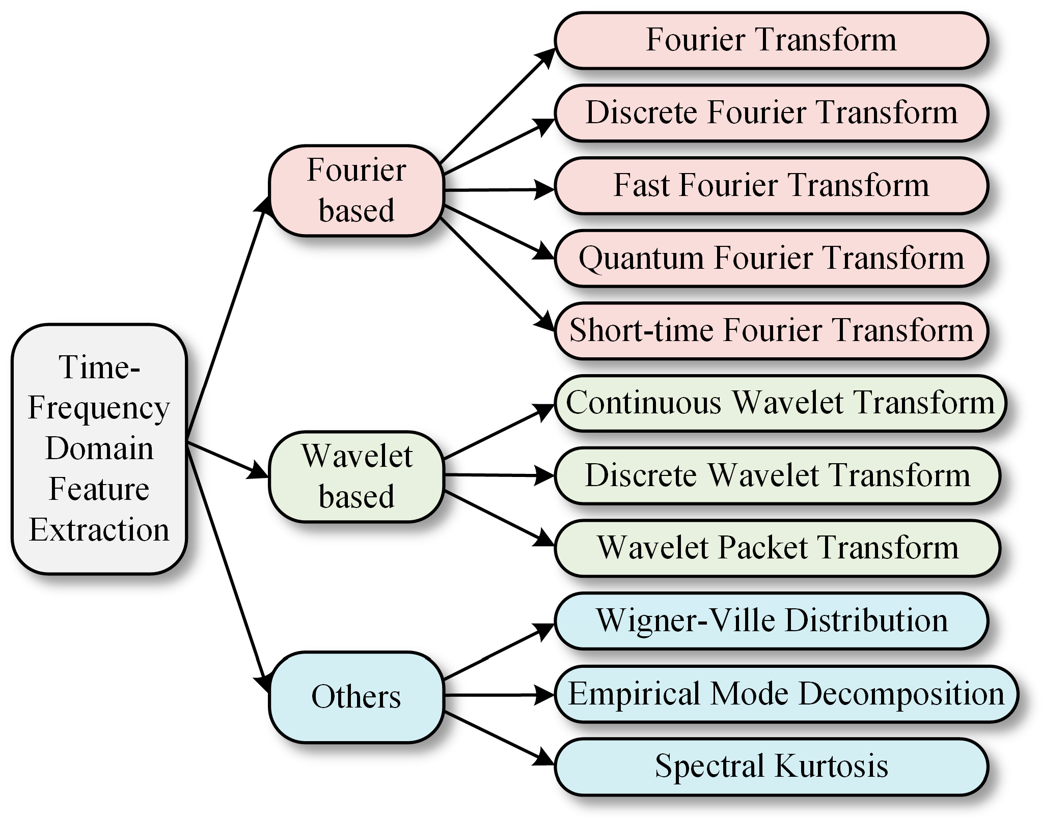
Currently, established time–frequency domain analysis methods encompass Fourier-based approaches [30], wavelet-based techniques, and others (see Figure 2). The fundamental principle of these methods involves segmenting the sequence into small, fixed-length segments, allowing for the determination of the spectral distribution trend of the entire time series through the processing of each segment.
In this paper, the discrete wavelet transform (DWT) is applied to segment the original sequence. DWT engages wavelet basis functions that convolve with a signal, decomposing it into components across different scales. This methodology facilitates analysis of the signal at varying resolutions, enabling the capture of both detailed (high-frequency) and smooth (low-frequency) components. By examining these components, the characteristics of the original signal at different scales can be effectively extracted. The wavelet function of the DWT used in this paper can be expressed as:
ψ m , n ( t ) = 1 a 0 m ψ ( t n τ 0 a 0 m a 0 m ) = 1 a 0 m ψ ( a 0 m t n τ 0 )
where a represents the scaling factor in the time–frequency domain, corresponding to the scaling characteristics of wavelet functions. τ is the translation factor in the time–frequency domain, corresponding to the time-shift characteristics of the wavelet function. ψ signifies the mother wavelet. The variables m and n are the integer values that control the scaling and translating.
The corresponding DWT can be expressed as:
W f ( m , n ) = + f ( t ) ψ m , n ( t ) d t
Based on (8), the maximum overlap discrete wavelet transform (MODWT) is employed to ensure that the transformed sequence retains the same length as the original signal, thereby circumventing the limitations of the DWT regarding the length of input signals [31]. This characteristic enhances the adaptability of the time–frequency domain feature extraction method proposed in this paper. The mathematical formulation of MODWT is presented as follows.
Wavelet coefficient:
W j , l = l = 0 L j 1 h j , l ˜ X t - l m o d N
Scaling coefficient:
V j , l = l = 0 L j 1 g j , l ˜ X t - l m o d N
here, h j , l and g j , l signify the wavelet and scaling filter of MODWT, respectively. j and l are defined as the level of decomposition and length of the filter ( l = 1 , 2 , , L ) with L j = ( 2 j 1 ) ( L 1 ) .
Using MODWT decomposition, the original signal can be decomposed into a series of components (level 1 to n) and approximate signals. For discrete signals, the energy is defined as the sum of the squares of the individual sampling points. In contrast, for continuous signals, the energy is calculated as the integral of the square over the entire interval of the signal. In feature engineering contexts, components with higher energy are typically selected to minimize information loss. In the case of DC signals, such as the converter output voltage discussed in this paper, the approximate signal generally contains the most energy. Consequently, this approximated signal is extracted, and its envelope is obtained using the Hilbert transform.
The Hilbert transform is defined as the convolution of the original signal with 1 π t , as shown in (11). Thereby, the Hilbert transform can be treated as a quadrature filter.
x ( t ) = H [ x ( t ) ] = + x ( t ) t τ d τ π = x ( t ) 1 π t
A new analytic signal can be defined as
z ( t ) = x ( t ) + j x ( t )
For a signal with amplitude and phase, x ( t ) can be written as x ( t ) = a ( t ) cos ( w 0 t + θ ( t ) ) , therefore, (12) becomes (13):
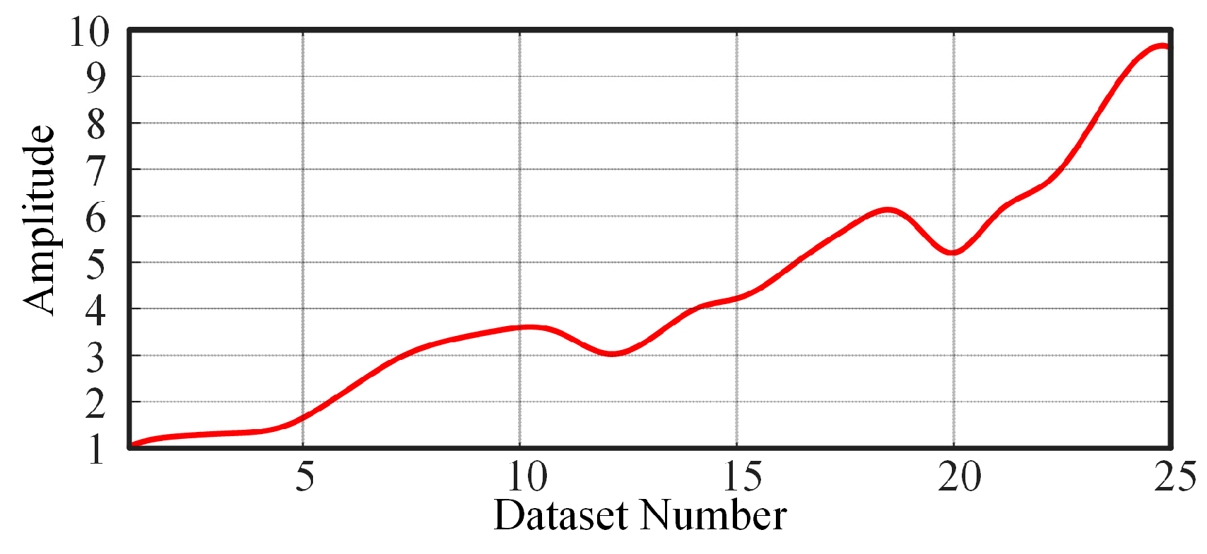
z ( t ) = a ( t ) cos ( w 0 t + θ ( t ) ) + j a ( t ) sin ( w 0 t + θ ( t ) ) = a ( t ) e j ( w 0 t + θ ( t ) ) = a ( t ) e j w 0 t e j θ ( t )
In (13), z ( t ) = a ( t ) e j w 0 t e j θ ( t ) = a ( t ) is the envelope of the original signal. The difference between the upper and lower envelopes can then be taken as a degradation feature in the time–frequency domain.

2.4. Feature Selection Method

The features can be broadly categorized into three groups: (a) noisy and irrelevant, (b) redundant or weakly related, and (c) strongly related. The primary objective of feature selection is to create an optimal subset of features from the original feature set that maximizes relevance while minimizing redundancy. As a data dimensionality reduction technique, feature selection aims to enhance learning performance, improve accuracy, reduce computational costs, and increase model interpretability.
Feature selection methods can be classified into three main categories: supervised, unsupervised, and semi-supervised algorithms. Commonly used supervised algorithms can be further divided into filters, embedded methods, hybrid methods, and wrappers. The feature selection method proposed in this paper is based on the ReliefF algorithm, which is a supervised filtering method.
The ReliefF algorithm is a multi-class feature weighting algorithm derived from the Relief method, which assigns different weights to features based on their relevance to different classes. ReliefF algorithm randomly selects a sample x r from the training set and then finds the nearest neighbor sample of the same class (called the near hit) x h i t , and the nearest neighbor sample of a different class (called the near miss) x m i s s . ReliefF algorithm firstly sets all the feature weights W j to 0 and then updates these weights based on the distances between these two samples.
For near hit:
W j i = W j i 1 Δ j ( x r , x h i t ) m d r h i t
For near miss:
W j i = W j i 1 P y m i s s 1 P y r Δ j ( x r , x m i s s ) m d r m i s s
where W j i and W j i 1 are the weights of features at the i -th and ( i 1 ) -th iteration steps, respectively. Δ j ( x r , x h i t ) and Δ j ( x r , x m i s s ) denote the difference between sample set x r and its nearest neighbor ( x h i t , x m i s s ) . m is the number of iterations. P y m i s s is the prior probability of the class to which x m i s s belongs, and P y r is the prior probability of the class to which x r belongs. d r h i t and d r m i s s are the distance function.
From (14) and (15), it is evident that if a feature demonstrates strong relevance in distinguishing near hits from near misses, its weight will be increased; conversely, if the feature exhibits a weak correlation, its weight will be decreased. The ReliefF algorithm accommodates both nominal and numerical variables and allows for the specification of a threshold or a predetermined number of important features. The running time of the algorithm increases linearly with the number of samples and the original feature dimensions.
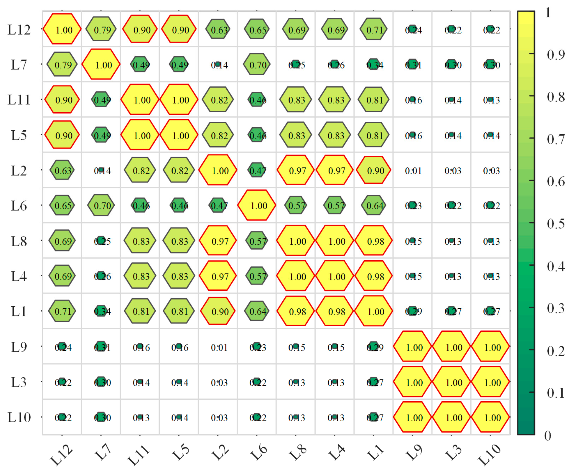
The ReliefF algorithm effectively calculates the correlation between features and targets, specifically, the correlation between the feature set x and the supervisory quantity y 
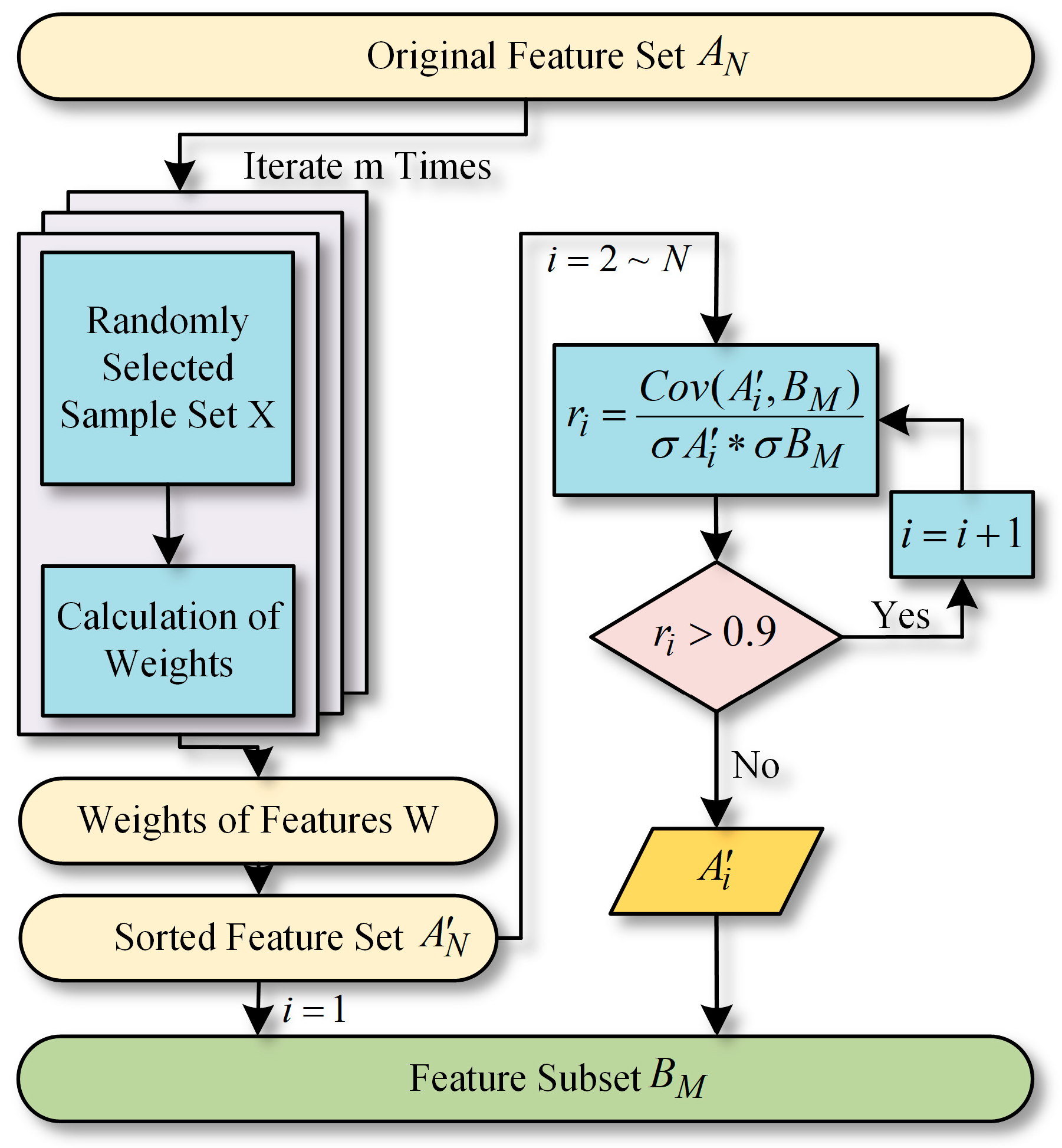
. However, it does not account for the correlation among features, which can lead to the inclusion of highly redundant features with strong correlations in the selected feature subset. To address this limitation, this paper proposes an improved feature selection method that builds upon the ReliefF algorithm and is enhanced by the Pearson correlation coefficient. After determining the weights of the original feature set, the algorithm conducts a correlation analysis on each feature prepared for inclusion in the selected feature subset, subsequently removing redundant features. This approach ensures that only the most relevant and significant features are retained in the final feature subset, thereby enhancing the accuracy and efficiency of subsequent training and processing. The flowchart of the algorithm is illustrated in Figure 3.
The proposed ReliefF–Pearson algorithm first weights the features using the ReliefF algorithm to generate a sorted feature set. The highest-ranked feature is directly added to the selected feature subset. For subsequent features, the Pearson correlation coefficient between each feature and the existing feature subset is calculated. If this correlation exceeds a predefined threshold, the feature is discarded; otherwise, it is included in the selected feature subset.

3. Implementation

3.1. Construction of Experimental Platform

This article focuses on the development of an interleaved Boost converter as the primary research object. The interleaved topology (illustrated in Figure 4) effectively enhances the power level while reducing the ripple amplitude compared to traditional single-phase converters. This topology is increasingly being adopted in aerospace power systems.
The converter designed in this study achieves a voltage conversion from 50 V to 80 V at a power level of 250 W, operating with a switching frequency of 80 kHz in continuous conduction mode (CCM), and utilizes a control system based on a Xilinx FPGA.
Figure 4 illustrates that certain breakpoints are established within the power circuit to facilitate the injection of simulated degradation parameters, such as the equivalent series resistance (ESR) of the output electrolytic capacitor and the on-resistance of the MOSFET. According to statistics [32], capacitor failures in the converter account for approximately 60% of overall failures, highlighting that capacitors are the most sensitive components regarding converter degradation. A key characteristic of the degradation process of capacitors is the increase in ESR [33]. Consequently, this paper simulates the degradation process of the output capacitor using a series of resistors, which effectively represent the degradation state of the converter. The degradation characteristics in the output electrical parameters are investigated through multi-domain feature extraction methods.
There are three commonly used PHM methods, namely model-based methods, data-driven methods, and knowledge-based methods [34,35]. The feature extraction method presented in this paper is data-driven, so acquiring data is the most basic step. A simulated degradation test bench for the interleaved boost converter was set up to obtain raw data on the output voltage (as shown in Figure 5).

3.2. Data Acquisition

The degradation process of the output capacitor’s ESR is simulated in this paper by connecting precision resistors of varying resistance in series with the anode of the electrolytic capacitor. The output capacitor utilized in this study has a rated internal resistance of approximately 10 mΩ, and the resistance value is primarily dependent on temperature over a limited duration. Consequently, these values remain virtually constant at room temperature under stable operating conditions. Therefore, the ESR of the output filter capacitor at different stages of degradation is approximated by the resistance of the series resistor. The selected series resistors used in this study are detailed in Table 2.
Considering the testability under actual conditions, the output voltage is chosen as the primary data source for feature extraction. The pre-processing of the original data primarily involves the removal of abnormal zero values and denoising. The output voltage waveform of the testing circuit with typical series resistors is illustrated in Figure 6. Subtle differences between these waveforms can be quantified through feature extraction. It is important to note that the sampling frequency employed in this study is 500 MHz.

4. Feature Extraction and Validation

4.1. Time Domain Features

In the time domain feature extraction of this article, five dimensional parameters (maximum value, minimum value, mean value, peak-to-peak value, and variance) and three dimensionless parameters (kurtosis, skewness, and crest factor) were extracted.
After normalization, the result of feature extraction in the time domain is shown in Figure 7. Several parameters of the converter output voltage exhibit distinct regular shifts, particularly the variance. This phenomenon can be attributed to the operating mechanism of the converter; as the ESR increases, the stabilizing effect of the output capacitor on the voltage gradually diminishes, resulting in increased voltage fluctuations. The variation in output voltage ripple serves as a significant indicator of converter degradation.

4.2. Frequency Domain Features

By performing FFT decomposition on the output voltage, the results presented in Figure 8 can be obtained. It is evident that the harmonic components in the output voltage are relatively low, making it challenging to differentiate the output voltage at various ESRs based solely on the amplitude of a specific harmonic.
Figure 9 illustrates the variation in the frequency domain features. The mean and variance curves of the power spectrum do not exhibit intuitive regularity. This observation suggests that the effects of converter degradation may not be adequately reflected in the energy spectrum, possibly due to the limited variation of ESR within a narrow range. Notably, a clear trend of decreasing harmonic distortion is observed. As the equivalent ESR gradually increases, the harmonic distortion of the output voltage ripple decreases from 9.9997 × 10 6 to 9.997 × 10 6 , representing a decrease of 0.027%. This observation indicates a decreasing trend; however, the relative amount of change is minimal.

4.3. Time–Frequency Domain Features

This paper integrates 25 sets of output voltage curves to examine the aging process of capacitors’ ESR, simulating the degradation of the converter’s output voltage as the output filtering capacitor deteriorates. Wavelet decomposition is fundamentally similar to FFT decomposition in the frequency domain; however, the frequency of the decomposed signal can only reach up to half of the sampled data points, meaning the frequency range corresponding to the decomposed signal is limited to 0–0.5. After six layers of decomposition, the original signal is transformed into seven new signals (level 1 to 6 signals and the approximate signal). The output voltage of the converter is a DC signal, indicating that the sample sequences oscillate around a fixed value. Consequently, the level 1 to 6 signals obtained from the decomposition oscillate around 0 (see Figure 10), containing only a minimal amount of energy. Notably, 97.2% of the original signal energy is concentrated in the approximate signal.
Figure 11 illustrates that the centerline of the approximate data closely resembles that of the raw data, indicating that the approximated data retains much of the original information. Furthermore, a distinct degradation trend is evident in the approximated data, characterized by a gradual increase in oscillation amplitude. The envelope effectively represents this changing trend. Therefore, the Hilbert transform is employed in this paper to process the approximate data and extract its envelope. The difference between the upper and lower envelopes is utilized as a feature in the time-frequency domain, as depicted in Figure 12.

4.4. Feature Selection and Performance Evaluation

The features extracted in the time domain, frequency domain, and time–frequency domain are presented in Table 3. Generally, time and frequency domain features necessitate less data and do not require continuous and complete system degradation curves. In contrast, time–frequency domain features can more accurately reflect the degradation state of the system; however, they require comprehensive degradation process data, making them suitable for scenarios where periodic sampling is conducted throughout the life cycle. To streamline the training process of the incipient fault diagnosis model and enhance operational efficiency, it is essential to select the original feature set. After the operation of the ReliefF algorithm, the features are given different weights, and the results obtained are shown in Table 3.
As previously mentioned, the required feature subset cannot be directly formed by selecting features with higher weights (top ranked) because the ReliefF algorithm does not account for the internal correlations among the features. Consequently, it is essential to perform a correlation test, as outlined in Figure 3. In this paper, the Pearson correlation coefficient is employed to conduct the correlation test between the features.
The Pearson correlation coefficient r i ranges from [−1, 1]. A larger r i indicates a stronger correlation between the two variables. The correlation coefficient threshold selected in this paper is 0.9, which means that when r i > 0.9 , it is considered that the feature is highly correlated with the feature subset and should be discarded. While when r i 0.9 , it is considered that the feature has a high degree of independence and should be added to the feature subset.
The correlation test results presented in Figure 13 indicate that certain features exhibit strong correlations, such as L11 and L12, as well as L5 and L11. It is crucial to avoid selecting features with high correlations in the feature subset during the feature selection process. Based on the feature selection methodology outlined in this paper, the final circuit degradation features identified are L12, L7, L2, and L6.
An incipient fault diagnosis model is established using a BPNN to validate the performance of the selected feature subset. In this model, the input parameters consist of the circuit degradation features identified in the previous section, while the output parameter is the assessed current circuit health. The BPNN employs a fully connected network structure, facilitating non-linear mapping between inputs and outputs and demonstrating robust generalization capabilities.
The entire dataset was divided into 25 groups; 20 groups were randomly selected as the training set, while the remaining 5 groups were designated as the testing set. This process was repeated five times to ensure the reliability of the results.
The hardware environment used for the validation of this paper consists of an Intel Core i5-8400 CPU with a clock speed of 2.80 GHz, while the software environment is MATLAB 2018b. In this paper, time is defined as the duration required to train the network parameters using the Levenberg–Marquardt gradient descent algorithm until optimal performance is achieved, with 20 groups of training set samples being utilized. Performance is measured by the mean squared error (MSE) between the model output and the sample labels when five groups of test sets are introduced into the trained BPNN model. Given that the number of nodes in the hidden layer of a neural network influences both training speed and performance, this study compares configurations with three hidden layers and five hidden layers, respectively. Through five iterations of training and validation, it was observed that, regardless of the network structure, the subset of selected features significantly outperforms the original feature set, which includes all features, in terms of model training speed, while the difference in training performance is minimal. To mitigate random errors associated with a single experiment, the average of the five results is illustrated by the red dashed line in Figure 14. This outcome convincingly demonstrates that the feature extraction and selection process proposed in this paper can effectively enhance model operational efficiency and simplify the model structure while also ensuring the accuracy of the output results.

5. Discussion

The proposed converter incipient fault feature extraction process in this paper represents a significant step forward in addressing the challenges associated with early fault detection in various industrial and technological sectors. By focusing on both time and frequency domains, as well as introducing a novel time–frequency domain feature, the methodology ensures a comprehensive analysis that captures a wide range of fault signatures. This comprehensive approach minimizes information loss and enhances the reliability of fault detection systems. The improved feature selection method, combining ReliefF with the Pearson correlation coefficient, is an innovative approach to reducing redundancy in the feature subset. This method not only ensures that the most relevant features are selected but also streamlines the feature set, which can significantly improve the computational efficiency of the subsequent fault diagnosis model.
Despite its many strengths, the proposed methodology may have certain limitations. For instance, the effectiveness of the feature extraction and selection process may depend on the specific nature of the faults being detected and the operating conditions of the converter. Additionally, while the use of wavelet decomposition for deriving the novel time–frequency domain feature is innovative, it may introduce computational complexity that needs to be carefully managed, especially in real-time applications. Overall, the proposed methodology offers a promising framework for incipient fault detection in converters and holds significant potential for broader applications in prognosis and health management across multiple industries.

6. Conclusions

The converter incipient fault feature extraction process proposed in this paper encompasses two main aspects, feature extraction and selection, representing a commendable approach. Eight features are extracted from the time domain and three from the frequency domain. Furthermore, this paper introduces a novel time–frequency domain feature, which is derived from the difference between the upper and lower envelopes of the approximated signal obtained through wavelet decomposition of the original voltage. Subsequently, an improved feature selection method is proposed, based on the ReliefF method and enhanced by the Pearson correlation coefficient, effectively reducing redundancy within the selected feature subset. The neural network-based incipient fault diagnosis model demonstrates that the chosen feature subset significantly enhances the training speed of the model while maintaining its accuracy.
The methodology outlined in this paper thoroughly addresses features across the time, frequency, and time–frequency domains, thereby minimizing information loss. The concepts and techniques presented are applicable to prognosis and health management in sectors such as aerospace, maritime, and electric vehicles.

Author Contributions

Methodology, C.Z.; Validation, P.G.; Investigation, M.H. and W.L. (Weilin Li); Resources, W.L. (Weilin Li); Writing—original draft, C.Z.; Writing—review & editing, W.L. (Wenjie Liu); Supervision, X.Z.; Project administration, X.Z. All authors have read and agreed to the published version of the manuscript.

Funding

This research was funded in part by the Natural Science Basic Research Program of Shaanxi under Grant 2023-JC-QN-0599, in part by the National Natural Science Foundation of China under Grant 52307223.

Data Availability Statement

The raw data supporting the conclusions of this article will be made available by the athors on request.

Conflicts of Interest

The authors declare no conflict of interest.

References

  1. Atutxa, U.; Baraia-Etxaburu, I.; López, V.M.; González-Hernando, F.; Rujas, A. Multi-Objective Comparative Analysis of Active Modular Rectifier Architectures for a More Electric Aircraft. Aerospace 2022, 9, 98. [Google Scholar] [CrossRef]
  2. Back, A.; Chollet, P.; Fercoq, O.; Desgreys, P. Power-aware feature selection for optimized Analog-to-Feature converter. Microelectron. J. 2022, 122, 105386. [Google Scholar] [CrossRef]
  3. Givi, H.; Farjah, E.; Ghanbari, T. Switch and diode fault diagnosis in nonisolated DC–DC converters using diode voltage signature. IEEE Trans. Ind. Electron. 2017, 65, 1606–1615. [Google Scholar] [CrossRef]
  4. Zhuo, S.; Gaillard, A.; Xu, L.; Liu, C.; Paire, D.; Gao, F. An observer-based switch open-circuit fault diagnosis of DC–DC converter for fuel cell application. IEEE Trans. Ind. Appl. 2020, 56, 3159–3167. [Google Scholar] [CrossRef]
  5. Zio, E. Prognostics and Health Management (PHM): Where are we and where do we (need to) go in theory and practice. Reliab. Eng. Syst. Saf. 2021, 218, 108119. [Google Scholar] [CrossRef]
  6. Rohan, A. Holistic Fault Detection and Diagnosis System in Imbalanced, Scarce, Multi-Domain (ISMD) Data Setting for Component-Level Prognostics and Health Management (PHM). Mathematics 2022, 10, 2031. [Google Scholar] [CrossRef]
  7. Nguyen, K.T.P.; Medjaher, K.; Tran, D.T. A review of artificial intelligence methods for engineering prognostics and health management with implementation guidelines. Artif. Intell. Rev. 2022, 56, 3659–3709. [Google Scholar] [CrossRef]
  8. Song, J.; Cho, S.H.; Kim, S.; Na, J.; Choi, J.-H. A Comparative Study of Data-Driven Prognostic Approaches under Training Data Deficiency. Aerospace 2024, 11, 741. [Google Scholar] [CrossRef]
  9. Guo, L.; Li, N.; Jia, F.; Lei, Y.; Lin, J. A recurrent neural network based health indicator for remaining useful life prediction of bearings. Neurocomputing 2017, 240, 98–109. [Google Scholar] [CrossRef]
  10. Zhou, S.; He, Z.; Chen, X.; Chang, W. An Anomaly Detection Method for UAV Based on Wavelet Decomposition and Stacked Denoising Autoencoder. Aerospace 2024, 11, 393. [Google Scholar] [CrossRef]
  11. Kong, J.-z.; Yang, F.; Zhang, X.; Pan, E.; Peng, Z.; Wang, D. Voltage-temperature health feature extraction to improve prognostics and health management of lithium-ion batteries. Energy 2021, 223, 120114. [Google Scholar] [CrossRef]
  12. Nayana, B.R.; Geethanjali, P. Improved Identification of Various Conditions of Induction Motor Bearing Faults. IEEE Trans. Instrum. Meas. 2020, 69, 1908–1919. [Google Scholar] [CrossRef]
  13. Han, W.; Cheng, L.; Han, W.; Yu, C.; Yin, Z.; Hao, Z.; Zhu, J. Incipient Fault Diagnosis for DC–DC Converter Based on Multi-Dimensional Feature Fusion. IEEE Access 2023, 11, 58822–58834. [Google Scholar] [CrossRef]
  14. Udmale, S.S.; Singh, S.K. Application of Spectral Kurtosis and Improved Extreme Learning Machine for Bearing Fault Classification. IEEE Trans. Instrum. Meas. 2019, 68, 4222–4233. [Google Scholar] [CrossRef]
  15. Tian, J.; Morillo, C.; Azarian, M.H.; Pecht, M. Motor bearing fault detection using spectral kurtosis-based feature extraction coupled with K-nearest neighbor distance analysis. IEEE Trans. Ind. Electron. 2015, 63, 1793–1803. [Google Scholar] [CrossRef]
  16. Li, H.; Liu, T.; Wu, X.; Chen, Q. Application of EEMD and improved frequency band entropy in bearing fault feature extraction. ISA Trans. 2019, 88, 170–185. [Google Scholar] [CrossRef] [PubMed]
  17. Yang, J.; Wu, C.; Shan, Z.; Liu, H.; Yang, C. Extraction and enhancement of unknown bearing fault feature in the strong noise under variable speed condition. Meas. Sci. Technol. 2021, 32, 105021. [Google Scholar] [CrossRef]
  18. Anderson, R.; Sandsten, M. Classification of EEG signals based on mean-square error optimal time-frequency features. In Proceedings of the 2018 26th European Signal Processing Conference (EUSIPCO), Rome, Italy, 3–7 September 2018; pp. 106–110. [Google Scholar]
  19. Gandomi, A.A.; Kargar, M.; Kargar, S.; Parsa, L.; Corzine, K. Deep-Learning-based Fault Detection and Location Method Applied on Isolated Dc-Dc Converter. In Proceedings of the 2023 IEEE Applied Power Electronics Conference and Exposition (APEC), Orlando, FL, USA, 19–23 March 2023; pp. 2245–2252. [Google Scholar]
  20. Cui, J.; Shi, G.; Zhang, Z. Fault detection of aircraft generator rotating rectifier based on SAE and SVDD method. In Proceedings of the 2017 Prognostics and System Health Management Conference (PHM-Harbin), Harbin, China, 9–12 July 2017; pp. 1–5. [Google Scholar]
  21. Bandyopadhyay, I.; Purkait, P.; Koley, C. Performance of a Classifier Based on Time-Domain Features for Incipient Fault Detection in Inverter Drives. IEEE Trans. Ind. Inform. 2019, 15, 3–14. [Google Scholar] [CrossRef]
  22. Wang, X.; Sui, G.; Xiang, J.; Wang, G.; Huo, Z.; Huang, Z. Multi-Domain Extreme Learning Machine for Bearing Failure Detection Based on Variational Modal Decomposition and Approximate Cyclic Correntropy. IEEE Access 2020, 8, 197711–197729. [Google Scholar] [CrossRef]
  23. Yang, J.; Yang, Y.; Xie, G. Diagnosis of Incipient Fault Based on Sliding-Scale Resampling Strategy and Improved Deep Autoencoder. IEEE Sens. J. 2020, 20, 8336–8348. [Google Scholar] [CrossRef]
  24. Li, Q.; Luo, H.; Cheng, H.; Deng, Y.; Sun, W.; Li, W.; Liu, Z. Incipient Fault Detection in Power Distribution System: A Time–Frequency Embedded Deep-Learning-Based Approach. IEEE Trans. Instrum. Meas. 2023, 72, 1–14. [Google Scholar] [CrossRef]
  25. Deng, F.; Jin, M.; Liu, C.; Liserre, M.; Chen, W. Switch Open-Circuit Fault Localization Strategy for MMCs Using Sliding-Time Window Based Features Extraction Algorithm. IEEE Trans. Ind. Electron. 2021, 68, 10193–10206. [Google Scholar] [CrossRef]
  26. Xiao, D.; Lin, Z.; Yu, A.; Tang, K.; Xiao, H. Data-driven method embedded physical knowledge for entire lifecycle degradation monitoring in aircraft engines. Reliab. Eng. Syst. Saf. 2024, 247, 110100. [Google Scholar] [CrossRef]
  27. Saleem, U.; Liu, W.; Li, W.; Sardar, M.U.; Aslam, M.M.; Riaz, S. Enhancing PHM System of Aircraft Generator with Machine Learning-Driven Faults Classification. In Proceedings of the 2024 ASU International Conference in Emerging Technologies for Sustainability and Intelligent Systems (ICETSIS), Manama, Bahrain, 28–29 January 2024; pp. 1–5. [Google Scholar]
  28. Zhang, Y.; Hanachi, H.; Liu, J.; Yang, C. Model-based Degradation Inference for Auxiliary Power Unit Start System. Eng. Fail. Anal. 2020, 118, 104895. [Google Scholar] [CrossRef]
  29. Prost, J.; Boidi, G.; Varga, M.; Vorlaufer, G.; Eder, S.J. Lifetime assessment of porous journal bearings using joint time-frequency analysis of real-time sensor data. Tribol. Int. 2022, 169, 107488. [Google Scholar] [CrossRef]
  30. Ehya, H.; Skreien, T.N.; Nysveen, A. Intelligent Data-Driven Diagnosis of Incipient Interturn Short Circuit Fault in Field Winding of Salient Pole Synchronous Generators. IEEE Trans. Ind. Inform. 2022, 18, 3286–3294. [Google Scholar] [CrossRef]
  31. Patnaik, B.; Mishra, M.; Bansal, R.C.; Jena, R.K. MODWT-XGBoost based smart energy solution for fault detection and classification in a smart microgrid. Appl. Energy 2021, 285, 116457. [Google Scholar] [CrossRef]
  32. Lahyani, A.; Venet, P.; Grellet, G.; Viverge, P.J. Failure prediction of electrolytic capacitors during operation of a switchmode power supply. IEEE Trans. Power Electron. 1998, 13, 1199–1207. [Google Scholar] [CrossRef]
  33. Yu, Y.; Jiang, Y.; Liu, Y.; Peng, X. Incipient fault diagnosis method for DC-DC converters based on sensitive fault features. IET Power Electron. 2020, 13, 4646–4658. [Google Scholar] [CrossRef]
  34. Kordestani, M.; Orchard, M.E.; Khorasan, K.; Saif, M. An Overview of the State-of-the-Art in Aircraft Prognostic and Health Management Strategies. IEEE Trans. Instrum. Meas. 2023, 72, 3505215. [Google Scholar] [CrossRef]
  35. Dong, G.; Yang, F.; Wei, Z.; Wei, J.; Tsui, K.L. Data-Driven Battery Health Prognosis Using Adaptive Brownian Motion Model. IEEE Trans. Ind. Inform. 2020, 16, 4736–4746. [Google Scholar] [CrossRef]
Figure 1. Framework of the proposed research process.
Aerospace 11 01027 g001
Figure 2. Feature extraction methods in time–frequency domain.
Aerospace 11 01027 g002
Figure 3. The flowchart of the ReliefF–Pearson algorithm.
Aerospace 11 01027 g003
Figure 4. Topological structure of interleaved boost converter.
Aerospace 11 01027 g004
Figure 5. Experimental circuit and overall test environment. (a) Interleaved boost converter experimental circuit. (b) Experimental environment for simulating degradation.
Aerospace 11 01027 g005aAerospace 11 01027 g005b
Figure 6. Output voltage waveform of the testing converter with different series resistors. (a) Output voltage curve at ESR = 0 Ω. (b) Output voltage curve at ESR = 0.5 Ω. (c) Output voltage curve at ESR = 1.1 Ω.
Aerospace 11 01027 g006aAerospace 11 01027 g006b
Figure 7. Feature extraction results in time domain. (a) Dimensional feature extraction in time domain. (b) Dimensionless feature extraction in time domain.
Aerospace 11 01027 g007
Figure 8. Fast Fourier transform results of output voltage at different ESRs. (a) ESR = 0 Ω. (b) ESR = 0.5 Ω.
Aerospace 11 01027 g008
Figure 9. Feature extraction results in frequency domain. (a) Mean value of power spectrum. (b) Standard deviation of the power spectrum. (c) Harmonic distortion.
Aerospace 11 01027 g009
Figure 10. Result of MODWT.
Aerospace 11 01027 g010
Figure 11. Comparison of raw data and approximate data after wavelet decomposition.
Aerospace 11 01027 g011
Figure 12. Feature in time–frequency domain.
Aerospace 11 01027 g012
Figure 13. The results of correlation analysis.
Aerospace 11 01027 g013
Figure 14. Training results of the neural network. (a) Training process with 3 hidden layers. (b) Training process with 5 hidden layers.
Aerospace 11 01027 g014
Table 1. Commonly used time–domain dimensioned features.
IndexCalculation
Maximum value max ( x ( i ) )
Minimum value min ( x ( i ) )
Mean value 1 N i = 1 N x ( i )
Peak-to-peak value max ( x ( i ) ) min ( x ( i ) )
Variance 1 N i = 1 N x ( i ) μ 2
Table 2. The resistance of series resistors.
Num.Resistance
(Ω)
Num.Resistance
(Ω)
Num.Resistance
(Ω)
10100.37190.92
20.05110.42201
30.06875120.5211.05
40.08333130.55221.1
50.1140.6231.22
60.15150.65241.32
70.22160.72251.44
80.27170.77
90.32180.82
Table 3. The result of feature sorting.
Feature ParametersNomenclatureLabelRankingWeight
Max value of voltage V m a x L190.0265
Min value of voltage V m i n L250.0442
Mean value of voltage V m e a n L311−0.0277
Peak-to-peak value of voltage ripple V p e a k 2 p e a k L480.0332
Variance of voltage V v a r L540.0687
Kurtosis V k u r L660.0397
Skewness V s k e L720.0830
Crest factor V c f L870.0333
Mean value of power spectrum P s m e a n L910−0.0276
Standard deviation of power spectrum P s s t d L1012−0.0277
Harmonic distortion H D L1130.0688
Envelope of MODWT E n v o L1210.0899
Disclaimer/Publisher’s Note: The statements, opinions and data contained in all publications are solely those of the individual author(s) and contributor(s) and not of MDPI and/or the editor(s). MDPI and/or the editor(s) disclaim responsibility for any injury to people or property resulting from any ideas, methods, instructions or products referred to in the content.

