Adaptive Fast Smooth Second-Order Sliding Mode Fault-Tolerant Control for Hypersonic Vehicles

Abstract

In response to control issues in hypersonic vehicles under external disturbances, model uncertainties, and actuator failures, this paper proposes an adaptive fast smooth second-order sliding mode fault-tolerant control scheme. First, a system separation approach is adopted, dividing the hypersonic vehicle model into fast and slow loops for independent design. This ensures that the airflow angle tracking error and sliding mode variables converge to the vicinity of the origin within a finite time. A fixed-time disturbance observer is then designed to estimate and compensate for the effects of model uncertainties, external disturbances, and actuator failures. The controller parameters are dynamically adjusted through an adaptive term to enhance robustness. Furthermore, first-order differentiation is used to estimate differential terms, effectively avoiding the issue of complexity explosion. Finally, the convergence of the controller within a finite time is rigorously proven using the Lyapunov method, and the perturbation of aerodynamic parameters is tested using the Monte Carlo method. Simulation results under various scenarios show that compared with the terminal sliding mode method, the proposed method outperforms control accuracy and convergence speed. The root mean square errors for the angle of attack, sideslip angle, and roll angle are reduced by 65.11%, 86.71%, and 45.51%, respectively, while the standard deviation is reduced by 81.78%, 86.80%, and 45.51%, demonstrating that the proposed controller has faster convergence, higher control accuracy, and smoother output than the terminal sliding mode controller.

1. Introduction

Hypersonic vehicles (HSVs) fly at speeds exceeding 5 Mach, characterized by significant speed variations and extensive flight ranges [1,2]. HSVs are crucial in multiple nations’ military, political, and economic domains. However, the integrated structure of the HSV’s body and engine, coupled with the complex flight environment, results in the dynamic model of HSVs exhibiting characteristics such as uncertainty, strong coupling, rapid time variation, and intense nonlinearity [3,4,5]. Simultaneously, the complex flight conditions make HSVs susceptible to external disturbances. Non-lethal failures in the actuator can induce abrupt changes in HSV state variables, leading to a decrease in controller performance in mild cases and a complete loss of control in severe cases [6].

Therefore, designing effective control methods for external disturbances, model uncertainties, and actuator failures to endow HSVs with robustness and fault-tolerant control performance has become a crucial issue in the current research domain [7]. In recent years, nonlinear methods such as sliding mode control [8,9], performance-preserving control [10,11,12], intelligent control [13,14], etc., have been widely applied in the research of attitude control systems for HSVs.

To address external disturbances and modeling uncertainties in HSVs, academics have designed an adaptive controller based on the backstepping method, utilizing a sliding mode disturbance observer to estimate lumped disturbances precisely. However, this approach only considers the longitudinal model [15]. Guo et al. proposed a continuous nonsingular terminal sliding mode controller, employing a novel adaptive rate and utilizing the super-twisting sliding mode algorithm for disturbance estimation. Numerical simulations validated the method’s effectiveness, but actuator faults were not considered [16]. Cheng et al. proposed a predictive sliding mode control method based on feedback linearization, which mitigated the chattering phenomenon of sliding mode through a minimization approach to performance indices [17]. However, due to the intense nonlinearity characteristics of HSV, linearization often leads to significant modeling errors, making it challenging for the designed controller to ensure its performance across a wide range of operating conditions. Zhong et al. proposed an adaptive backstepping control method based on a super-twisting disturbance observer, incorporating a fixed-time anti-saturation compensator to mitigate the effects of actuator saturation, yet without addressing actuator faults [18]. Hu et al. considered the dynamic characteristics of the actuator, designing adaptive backstepping controllers and dynamic inverse controllers for the velocity and altitude subsystems, respectively, ensuring the convergence of the HSV’s attitude angles in the presence of aerodynamic uncertainties. However, this approach only considered the longitudinal model and did not address attitude control [19]. Cheng et al. addressed the longitudinal model of an HSV and designed a composite learning controller. It utilized a radial basis neural network to approximate lumped disturbances, constructed modeling errors to evaluate the quality of system learning, and validated the effectiveness of the control strategy through simulation, but similarly only considered the longitudinal model [20]. These studies also accounted for external disturbances and model uncertainties in their controller designs [21,22,23,24].

While the studies mentioned above have made some progress in controlling HSVs with external disturbances and modeling uncertainties, they have generally not considered the scenario of actuator failures. Further consideration is given to non-critical failures in the actuator system. Academics proposed an adaptive fault-tolerant approach based on output redefinition, confirming the non-minimum phase characteristics of the HSV, effectively compensating for the impact of actuator failures. However, this only considers the control of speed and altitude [25]. Shen et al. introduced a fault-tolerant control method based on Takagi-Sugeno fuzzy systems, compensating for the effects of actuator failures, but did not fully consider external disturbances [26]. Guo et al. considered additive and multiplicative faults in the actuators, proposing a fault-tolerant control method based on integral sliding mode [27]. Yuan et al. addressed the faults in deformation mechanisms in morphing aircraft and proposed an adaptive fault-tolerant control based on neural networks and L2 gain techniques. It utilized radial basis neural networks to compensate for system uncertainties [28]. Hu et al. proposed a novel adaptive fault-tolerant method, considering unknown time-varying faults in the elevators and throttle. They introduced a model with a smoothing function, estimating and compensating for the fault effects. However, the article focused solely on controlling the altitude and velocity of the HSV [29]. Lv et al. employed a feedback linearization approach to decouple the nonlinear model of HSVs into a linear model. They utilized a neural network observer to compensate for observed disturbances, including actuator failures, and designed an adaptive fixed-time nonsingular sliding mode fault-tolerant controller. However, the linear model is limited in accurately capturing the full dynamics of the aircraft [30]. These studies also addressed the fault-tolerant control issue in the presence of actuator failures [31,32,33].

However, in current research on hypersonic vehicle controllers, some studies have only focused on controllers for longitudinal models, overlooking the coupling effects of lateral motion. Additionally, there has been limited research on actuator faults under high-altitude and high-speed flight conditions, and the issues of actuator output smoothing and fast controller convergence have not been sufficiently considered. Since second-order sliding mode controllers offer faster dynamic responses than first-order controllers, they can effectively deal with external disturbances and system uncertainties, significantly reducing output chattering and smoother outputs. Therefore, we have considered modeling uncertainties, aerodynamic parameter uncertainties, external disturbances, and actuator faults and designed an adaptive fast smooth second-order sliding mode fault-tolerant controller (AFSSOSMFTC).

The main contributions of this work are outlined below:

(1)

Considering the coupling model between lateral and longitudinal dynamics of HSVs, we divide the model into fast and slow loop systems. Controllers and observers are designed for each loop to achieve control objectives.

(2)

The article proposed an AFSSOSMFTC method. It involves designing a fixed-time disturbance observer to estimate and compensate for aggregated disturbances and non-catastrophic faults in actuators. A first-order differentiator is also introduced to avoid the explosion of complexity. The controller parameters are dynamically adjusted through an adaptive term, enhancing the robustness of the controller.

This study validates the designed controller’s fast convergence and smooth output characteristics through numerical simulations. Nonlinear external disturbances and actuator faults are introduced to demonstrate the robustness and effectiveness of the fault-tolerant controller.

2. Establishment of the HSV Model

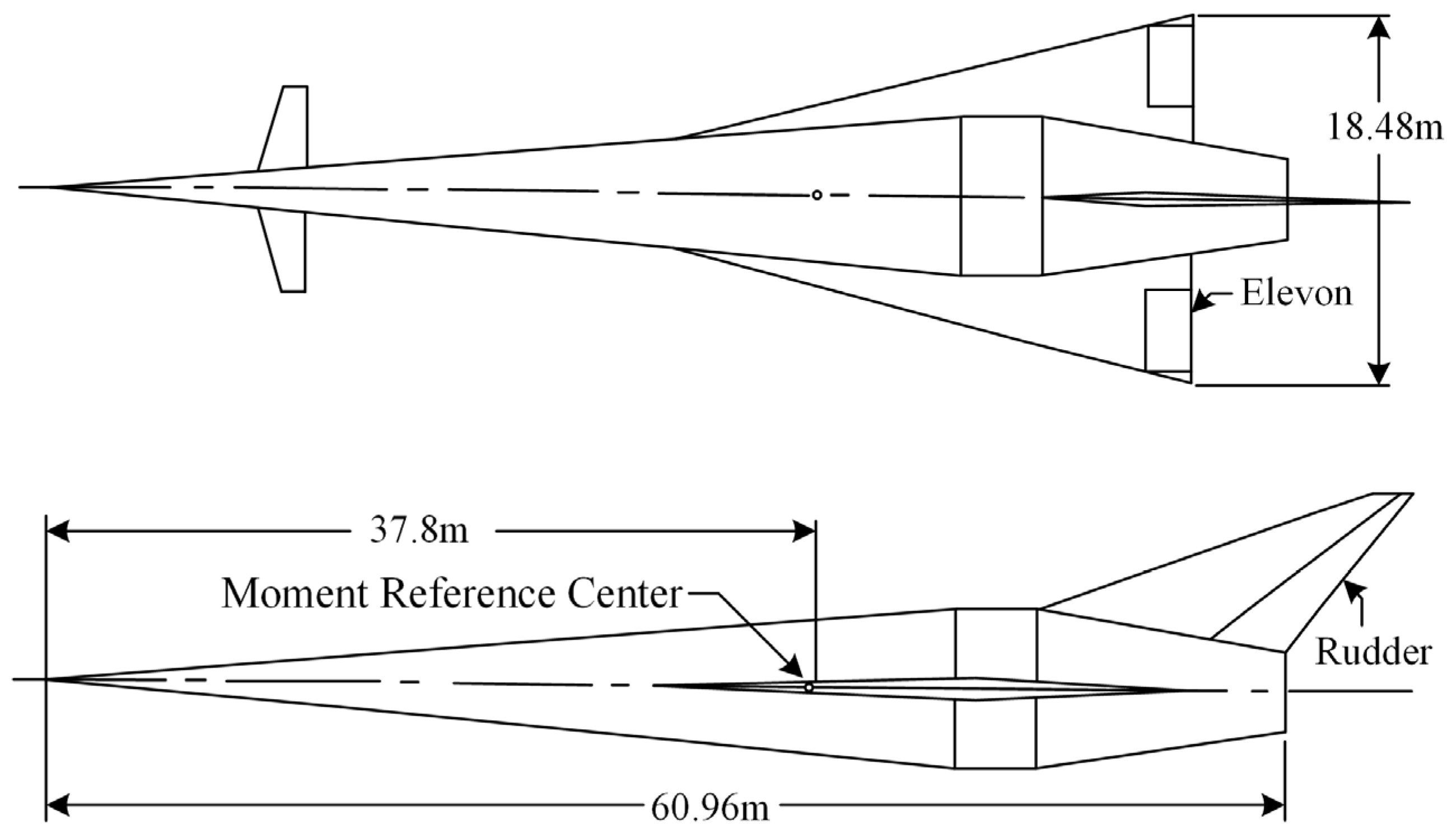
This article employs the generic conical HSV model (winged-cone) published by NASA Langley Research Center as the research subject. The geometric parameters of the model are illustrated in Figure 1 [34].

The establishment of the HSV attitude control model in the aerodynamic coordinate system is as follows:

$$\begin{array}{c}\dot{p}={\displaystyle \frac{I_y-I_z}{I_x}}rq+{\displaystyle \frac{1}{I_x}}l\hfill \\ \dot{q}={\displaystyle \frac{I_z-I_x}{I_y}}pr+{\displaystyle \frac{1}{I_y}}m\hfill \\ \dot{r}={\displaystyle \frac{I_x-I_y}{I_z}}pq+{\displaystyle \frac{1}{I_z}}n\hfill \\ \dot{\alpha }=q-p\cos \alpha \tan \beta -r\sin \alpha \tan \beta \hfill \\ \dot{\beta }=p\sin \alpha -r\cos \alpha \hfill \\ \dot{\chi }=-p\cos \alpha \cos \beta -q\sin \beta -r\sin \alpha \cos \beta \hfill \end{array}$$

(1)

where $p,q,r$ are the angular velocities about the three axes, and $\alpha ,\beta ,\chi$ represent the angle of attack, sideslip angle, and angle of bank, respectively. $l,m,n$ denote the rotational torques, and $I_x,I_y,I_z$ represent moment of inertia.

$$\begin{array}{c}l=bS{C}_l\rho V^2/2=bS{C}_l\overline{q}\\ m=\overline{c}S{C}_m\rho V^2/2=\overline{c}S{C}_m\overline{q}\\ n=bS{C}_n\rho V^2/2=bS{C}_n\overline{q}\end{array}$$

(2)

where $b,\overline{c}$ are the aerodynamic chord lengths, $\overline{q}$ is the dynamic pressure, and $C_l,C_m,C_n$ are the aerodynamic coefficients, defined as follows:

$$\begin{array}{l}{C}_l=C_l^{\beta }\beta +C_l^{{\delta }_a}{\delta }_a+C_l^{{\delta }_e}{\delta }_e+C_l^{{\delta }_r}{\delta }_r+C_l^p{\displaystyle \frac{pb}{2V}}+C_l^r{\displaystyle \frac{rb}{2V}}+{\Delta }_{C_l}\\ C_m=C_m^{\alpha }+C_m^{{\delta }_a}{\delta }_a+C_m^{{\delta }_e}{\delta }_e+C_m^{{\delta }_r}{\delta }_r+C_m^q{\displaystyle \frac{q\overline{c}}{2V}}+{\Delta }_{C_m}\\ C_n=C_n^{\beta }\beta +C_n^{{\delta }_a}{\delta }_a+C_n^{{\delta }_e}{\delta }_e+C_n^{{\delta }_r}{\delta }_r+C_n^p{\displaystyle \frac{pb}{2V}}+C_n^r{\displaystyle \frac{rb}{2V}}+{\Delta }_{C_n}\end{array}$$

(3)

where ${\Delta }_{C_l},{\Delta }_{C_m}$, and ${\Delta }_{C_n}$ represent the aerodynamic perturbation terms, and the attitude changes in HSV are influenced by the rotation of the actuator. The control distribution model is as follows:

$$C=\upsilon +\varsigma {\delta }_c$$

(4)

where

$$C=\left[\begin{array}{c}{C}_l\\ C_m\\ C_n\end{array}\right],\upsilon =\left[\begin{array}{c}{C}_l^{\beta }\beta +C_l^p{\displaystyle \frac{pb}{2V}}+C_l^r{\displaystyle \frac{rb}{2V}}\\ C_m^{\alpha }+C_m^q{\displaystyle \frac{q\overline{c}}{2V}}\\ C_n^{\beta }\beta +C_n^p{\displaystyle \frac{pb}{2V}}+C_n^r{\displaystyle \frac{rb}{2V}}\end{array}\right],\varsigma =\left[\begin{array}{ccc}{C}_l^{{\delta }_a}& C_l^{{\delta }_e}& C_l^{{\delta }_r}\\ C_m^{{\delta }_a}& C_m^{{\delta }_e}& C_m^{{\delta }_r}\\ C_n^{{\delta }_a}& C_n^{{\delta }_e}& C_n^{{\delta }_r}\end{array}\right],{\delta }_c=\left[\begin{array}{c}{\delta }_a\\ {\delta }_e\\ {\delta }_r\end{array}\right]$$

where $C_i^{{\delta }_j}$ and $C_i^k$ respectively represent the aerodynamic derivatives corresponding to the control surface and partial state variables about the three axes, and $i\in \left(l,m,n\right),j\in \left(a,e,r\right),k\in \left(\alpha ,\beta ,p,q,r\right)$; ${\delta }_a,{\delta }_e,{\delta }_r$ respectively represent the deflection of the pitch, roll, and yaw control surfaces.

The partial parameter information in the previous text is shown in

Table 1. HSV parameter table.

Parameter	Parameter Value
$S$	$334.7 ({\mathrm{m}}^2)$
$b$	$6.95 (\mathrm{m})$
$\overline{c}$	$24.384 (\mathrm{m})$
$I_x$	$1.36\times {10}^6 (\mathrm{k}\mathrm{g}\cdot {\mathrm{m}}^2)$
$I_y$	$1.36\times {10}^7 (\mathrm{k}\mathrm{g}\cdot {\mathrm{m}}^2)$
$I_z$	$1.36\times {10}^7 (\mathrm{k}\mathrm{g}\cdot {\mathrm{m}}^2)$

, and the remaining parameters can be referred to in the literature [34].

3. Control-Oriented HSV Model

Considering the uncertainties in the system and the presence of external disturbances, Equation (1) can be reformulated as follows:

$$\begin{array}{l}\dot{\Omega }=\eta \omega +{\Delta }_{\Omega }+d\\ \dot{\omega }=I^{-1}\left(\zeta I\omega +M\right)+{\Delta }_{\omega }\end{array}$$

(5)

where $\Omega ={\left[\begin{array}{ccc}\chi & \alpha & \beta \end{array}\right]}^T$, $\omega ={\left[\begin{array}{ccc}p& q& r\end{array}\right]}^T$, and ${\rm M}={\left[\begin{array}{ccc}l& m& n\end{array}\right]}^T$, with ${\Delta }_{\Omega },{\Delta }_{\omega }\in R^{3\times 1}$ representing the uncertainties in the system; $d\in R^{3\times 1}$ represents external disturbances, and the rest of the state matrices are expressed as follows:

$$\eta =\left[\begin{array}{ccc}-\cos \alpha \cos \beta & -\sin \beta & -\sin \alpha \cos \beta \\ -\cos \alpha \tan \beta & 1& -\sin \alpha \tan \beta \\ \sin \alpha & 0& -\cos \alpha \end{array}\right],\zeta =\left[\begin{array}{ccc}0& r& -q\\ -r& 0& p\\ q& -p& 0\end{array}\right],I=\left[\begin{array}{ccc}{I}_x& 0& 0\\ 0& I_y& 0\\ 0& 0& I_z\end{array}\right]$$

Substituting Equation (4) into Equation (5) yields the control model oriented to the control surfaces.

$$\begin{array}{l}\dot{\Omega }=\eta \omega +{\Delta }_{\Omega }+d\\ \dot{\omega }=I^{-1}\left[\zeta I\omega +\vartheta \left(\upsilon +\varsigma {\delta }_c\right)\right]+{\Delta }_{\omega }\end{array}$$

(6)

where $\mathit{\vartheta }=diag\left(bS\overline{q},\overline{c}S\overline{q},bS\overline{q}\right)$.

Considering unfavorable factors such as the complex and unpredictable actual flight environment of the aircraft, which can lead to failures in the HSV’s actuator, the following actuator fault model is established:

$$u_c=\left(1^{3\times 1}-\kappa \right){\delta }_c+u_{c0}$$

(7)

The above equation, $\kappa \in R^{3\times 1}$, represents the actuator efficiency fault, with a range of [0, 1]. When $\kappa =0^{3\times 1}$, it indicates no actuator efficiency fault, and when $\kappa =1^{3\times 1}$, it signifies complete actuator failure. ${\delta }_c$ represents the desired command signal given by the controller, $u_{c0}\in R^{3\times 1}$ denotes the control surface floating fault, and $u_c\in R^{3\times 1}$ is the actual control surface output command.

Further expansion yields:

$$\begin{array}{l}\dot{\Omega }=\eta \omega +{\Delta }_{\Omega }+d\\ \dot{\omega }=I^{-1}\left\{\zeta I\omega +\vartheta \left[\upsilon +\varsigma {\delta }_c+\varsigma \left(u_{c0}-\kappa {\delta }_c\right)\right]\right\}+{\Delta }_{\omega }\end{array}$$

(8)

4. Controller Design

This study aims to address the attitude control problem of HSVs in the presence of external disturbances and actuator faults. The control goals are as follows:

(1)

The controller should ensure the stability of the HSV in the presence of external disturbances and actuator faults.

(2)

Throughout the flight, the controller should effectively achieve continuous and stable tracking of target commands by the HSV.

By employing the concept of system separation, we can decompose the attitude control model of HSV into fast-loop and slow-loop subsystems for separate design. The fixed-time state observer estimates uncertainty, external disturbances, actuator faults, and other incalculable factors in the HSV model. The AFSSOSMFTC method is designed to achieve the aforementioned control objectives. Additionally, a first-order differentiator is employed to solve the derivatives of intermediate virtual control quantities, preventing the potential explosion of complexity.

4.1. Fixed-Time Disturbance Observer Design

A fixed-time disturbance observer is designed to address the parameter uncertainties and external aggregated disturbance terms ${\Delta }_{\Omega },{\Delta }_{\omega }$, and $d$ in the system presented in Equation (8). The design is as follows:

$$\left\{\begin{array}{l}{\dot{z}}_1=a_{1}si{g}^{m_1}\left(e\right)+b_{1}si{g}^{n_1}\left(e\right)+u+z_2\\ {\dot{z}}_2=a_{2}si{g}^{m_2}\left(e\right)+b_{2}si{g}^{n_2}\left(e\right)+r\tanh \left(e\right)\end{array}\right.$$

(9)

where $a_1,a_2,b_1,b_2$ and $r$ are the positive constants to be designed, $m_1,m_2\in \left(0,1\right),n_1,n_2>1$, and $m_2=2m_1-1,n_2=2n_1-1$. $si{g}^{n_i}\left(e\right)={\left|e\right|}^{n_i}sign\left(e\right),i=1,2$, and $si{g}^{m_i}\left(e\right)$ is the same as $si{g}^{n_i}\left(e\right)$. $sign\left(•\right)$ is the sign function, defined as follows:

$$sign\left(•\right)=\left\{\begin{array}{cc}1\hspace{1em}\hspace{1em}\hfill & \hfill if •>0\\ 0\hspace{1em}\hspace{1em}\hfill & \hfill if •=0\\ -1\hspace{1em}\hspace{1em}\hfill & \hfill if •<0\end{array}\right.$$

(10)

4.1.1. Controller Design Steps

In this section, controllers are separately designed for the slow loop and fast loop. The control system structure diagram is illustrated in Figure 2.

4.1.2. Integral Sliding Surface

Define the tracking errors for airflow angle and angular velocity as follows:

$$\left\{\begin{array}{l}{e}_{\Omega }=\Omega -{\Omega }_c\\ e_{\omega }=\omega -{\omega }_c\end{array}\right.$$

(11)

where ${\Omega }_c=\left[\begin{array}{ccc}{\chi }_c& {\alpha }_c& {\beta }_c\end{array}\right]$ is the airflow angle command signal, and ${\omega }_c=\left[\begin{array}{ccc}{p}_c& q_c& r_c\end{array}\right]$ is the intermediate virtual control variable for the slow-loop controller-produced angular velocity.

Choose the integral sliding surface as follows:

$$S=\left[\begin{array}{c}{s}_1\\ s_2\end{array}\right]=\left[\begin{array}{c}{e}_{\Omega }+c_1{\displaystyle {\int }_0^t{e}_{\Omega }\left(\tau \right)d\tau }\\ e_{\mathit{\omega }}+c_2{\displaystyle {\int }_0^t{e}_{\mathit{\omega }}\left(\tau \right)d\tau }\end{array}\right]$$

(12)

where $s_1$ and $s_2$ are the sliding surfaces for the slow loop and fast loop, and $c_1,c_2\in R$ are the sliding mode gains to be designed.

4.1.3. Controller Structure

The design of the AFSSOSMFTC is as follows:

$$\left\{\begin{array}{l}\dot{\xi }=-k_1{\left|\xi \right|}^{{\displaystyle \frac{j-1}{j}}}sign\left(\xi \right)-k_2\xi +\mathit{\epsilon }\\ \dot{\mathit{\epsilon }}=-k_3{\left|\xi \right|}^{{\displaystyle \frac{j-2}{j}}}sign\left(\xi \right)-k_4\xi \end{array}\right.$$

(13)

where $j>2$ is a constant, $k_i$ is the adaptive gain, and the adaptation rate is as follows:

$$\begin{array}{cc}{\dot{k}}_1=w_1‖e‖\sqrt{{\displaystyle \frac{{\mu }_1}{2}}}& {\dot{k}}_2=w_2‖e‖\sqrt{{\displaystyle \frac{{\mu }_2}{2}}}\\ {\dot{k}}_3=w_3‖e‖\sqrt{{\displaystyle \frac{{\mu }_3}{2}}}& {\dot{k}}_4=w_4‖e‖\sqrt{{\displaystyle \frac{{\mu }_4}{2}}}\end{array}$$

(14)

where $w_i>0,i=1,2,3,4$ are the gains of the adaptive terms, and ${\mu }_i>0$ are the constant terms to be designed. The value of $k_4$ is generally more prominent than $k_1$, $k_2$, and $k_3$, typically chosen to be above 10. The value of $k_1$ is usually less than or equal to $k_2$ and $k_3$ and generally kept within 10. The remaining parameters can be selected based on the saturation conditions.

In Equation (13), when the system’s sliding mode surface position is far from $\xi =0$, the convergence speed is mainly determined by the linear terms corresponding to $k_2$ and $k_4$. When the position is close to $\xi =0$, the convergence speed is primarily determined by the nonlinear terms corresponding to $k_1$ and $k_3$. Therefore, regardless of whether the system’s position $\xi$ is far from the equilibrium point, this method can converge to the equilibrium point at a relatively fast speed.

(1)

Design of the slow loop controller

Choosing $s_1$ as the slow loop sliding mode surface in Equation (12), differentiating it, and substituting it into Equations (8) and (11) yields the following:

$$\begin{array}{cc}\hfill {\dot{s}}_1& ={\dot{e}}_{\Omega }+c_1{e}_{\Omega }\hfill \\ & =\eta \omega +{\Delta }_{\Omega }+d-{\dot{\Omega }}_c+c_1{e}_{\Omega }\hfill \\ & =F_{\Omega }+d_{\Omega }+\eta \omega \hfill \end{array}$$

(15)

where $d_{\Omega }={\Delta }_{\Omega }+d$ represents the aggregated disturbance term in the slow loop, and $F_{\Omega }=c_1{e}_{\mathit{\Omega }}-{\dot{\Omega }}_c$.

Utilizing the fixed-time disturbance observer from Equation (9) to estimate the aggregated disturbance term $d_{\Omega }$, the design takes the following form:

$$\begin{array}{l}\dot{\widehat{\Omega }}=a_{11}si{g}^{m_{11}}\left(\widehat{\Omega }-\Omega \right)+b_{11}si{g}^{n_{11}}\left(\widehat{\Omega }-\Omega \right)+\eta {\omega }_c+{\widehat{d}}_{\Omega }\\ {\dot{\widehat{d}}}_{\Omega }=a_{12}si{g}^{m_{12}}\left(\widehat{\Omega }-\Omega \right)+b_{12}si{g}^{n_{12}}\left(\widehat{\Omega }-\Omega \right)+r_{1}tanh\left(\widehat{\Omega }-\Omega \right)\end{array}$$

(16)

where $\widehat{\Omega }$ and ${\widehat{d}}_{\Omega }$ respectively represent the estimated values of the airflow angle $\Omega$ and the aggregated disturbance term $d_{\Omega }$ in the slow loop system.

Defining the estimation error $\tilde{\Omega }=\widehat{\Omega }-\Omega$ and ${\tilde{d}}_{\Omega }={\widehat{d}}_{\Omega }-d_{\Omega }$, its dynamic error is given by the following expression:

$$\begin{array}{cc}\hfill \dot{\tilde{\Omega }}& =a_{11}si{g}^{m_{11}}\left(\tilde{\Omega }\right)+b_{11}si{g}^{n_{11}}\left(\tilde{\Omega }\right)+{\tilde{d}}_{\Omega }\hfill \\ \hfill {\dot{\tilde{d}}}_{\Omega }& =a_{21}si{g}^{m_{11}}\left(\tilde{\Omega }\right)+b_{21}si{g}^{n_{11}}\left(\tilde{\Omega }\right)+r\tanh \left(\tilde{\Omega }\right)-{\dot{d}}_{\Omega }\hfill \end{array}$$

(17)

Combining the control method in Equation (13), the slow loop sliding mode surface in Equation (15), and the disturbance observer in Equation (16), the design of the slow loop controller is as follows:

$$\begin{array}{cc}\hfill {\omega }_c& ={\eta }^{-1}\left(-k_1{\left|s_1\right|}^{{\displaystyle \frac{j_1-1}{j_1}}}sign\left(s_1\right)-k_2{s}_1-F_{\Omega }+{\widehat{d}}_{\Omega }+\epsilon \right)\hfill \\ \hfill \dot{\epsilon }& =-k_3{\left|s_1\right|}^{{\displaystyle \frac{j_1-2}{j_1}}}sign\left(s_1\right)-k_4{s}_1\hfill \end{array}$$

(18)

To avoid the potential explosion of complexity, the design incorporates a first-order filter to estimate the derivative term ${\dot{\mathit{\Omega }}}_c$ in the slow loop controller. The design takes the following form [3]:

$${\dot{\widehat{\Omega }}}_c=-{\displaystyle \frac{y_{\mathit{\Omega }}}{{\nu }_{\mathit{\Omega }}}}-{\displaystyle \frac{l_{1\mathit{\Omega }}{y}_{\mathit{\Omega }}}{{\left|y_{\mathit{\Omega }}\right|}^{\frac{1}{2}}+l_{2\mathit{\Omega }}}}$$

(19)

where ${\mathbf{\nu }}_{\mathit{\Omega }},l_{1\mathit{\Omega }},l_{2\mathit{\Omega }}>0$ are the parameters to be designed, and $y_{\mathit{\Omega }}={\hat{\mathit{\Omega }}}_c-{\mathit{\Omega }}_c$ represents the filtering error.

(2)

Design of the fast loop controller

Choosing $s_2$ as the fast loop sliding mode surface in Equation (12), differentiating it, and substituting it into Equations (8) and (11) yields the following:

$$\begin{array}{cc}\hfill {\dot{s}}_2& ={\dot{e}}_{\mathit{\omega }}+c_2{e}_{\mathit{\omega }}\hfill \\ & =I^{-1}\left\{\zeta I\mathit{\omega }+\mathit{\vartheta }\left[\upsilon +\varsigma {\delta }_c+\varsigma \left(u_{c0}-\kappa {\delta }_c\right)\right]\right\}+{\Delta }_{\omega }-{\dot{\mathit{\omega }}}_c+c_2{e}_{\mathit{\omega }}\hfill \\ & =F_{\mathit{\omega }}+d_{\mathit{\omega }}+I^{-1}\left[\zeta I\mathit{\omega }+\mathit{\vartheta }\left(\upsilon +\varsigma {\delta }_c\right)\right]\hfill \end{array}$$

(20)

where $d_{\mathit{\omega }}=I^{-1}\mathit{\vartheta }\varsigma \left(-\kappa {\delta }_c+u_{c0}\right)+{\Delta }_{\omega }$ represents the aggregated disturbance term due to rudder faults and uncertainties in the fast loop system, and $F_{\omega }=c_2{e}_{\omega }-{\dot{\mathit{\omega }}}_c$.

Designing a disturbance observer to estimate the aggregated disturbance term $d_{\omega }$ in the fast loop system provides the following:

$$\begin{array}{cc}\hfill \dot{\widehat{\omega }}& =a_{21}si{g}^{m_{21}}\left(\widehat{\omega }-\omega \right)+b_{21}si{g}^{n_{21}}\left(\widehat{\omega }-\omega \right)+I^{-1}\left[\zeta I\omega +\mathit{\vartheta }\left(\upsilon +\varsigma {\delta }_c\right)\right]+{\widehat{d}}_{\omega }\hfill \\ \hfill {\dot{\widehat{d}}}_{\omega }& =a_{22}si{g}^{m_{22}}\left(\widehat{\omega }-\omega \right)+b_{22}si{g}^{n_{22}}\left(\widehat{\omega }-\omega \right)+r_2\tanh \left(\widehat{\omega }-\omega \right)\hfill \end{array}$$

(21)

where $\widehat{\omega }$ and ${\widehat{d}}_{\omega }$ respectively represent the estimated values of the angle speed $\omega$ and the aggregated disturbance term $d_{\omega }$ in the fast loop system.

Defining the estimation error $\tilde{\omega }=\widehat{\omega }-\omega$ and ${\tilde{d}}_{\omega }={\widehat{d}}_{\omega }-d_{\omega }$, its dynamic error is given by the following expression:

$$\begin{array}{l}\dot{\tilde{\omega }}=a_{21}si{g}^{m_{21}}\left(\tilde{\omega }\right)+b_{21}si{g}^{n_{21}}\left(\tilde{\omega }\right)+{\tilde{d}}_{\omega }\\ {\dot{\tilde{d}}}_{\omega }=a_{21}si{g}^{m_{22}}\left(\tilde{\omega }\right)+b_{21}si{g}^{n_{22}}\left(\tilde{\omega }\right)+r_2\tanh \left(\tilde{\omega }\right)-{\dot{d}}_{\omega }\end{array}$$

(22)

The design of the fast loop controller is as follows:

$$\begin{array}{cc}\hfill {\delta }_c& ={\varsigma }^{-1}{\mathit{\vartheta }}^{-1}I(-k_1{\left|s_2\right|}^{{\displaystyle \frac{j_2-1}{j_2}}}sign\left(s_2\right)-k_2{s}_2-F_{\omega }+{\widehat{d}}_{\omega }+\epsilon )\hfill \\ & \hspace{1em}-{\varsigma }^{-1}{\mathit{\vartheta }}^{-1}\zeta I\mathit{\omega }-{\varsigma }^{-1}\upsilon dd\hfill \\ \hfill \dot{\epsilon }& =-k_3{\left|s_2\right|}^{{\displaystyle \frac{j_2-2}{j_2}}}sign\left(s_2\right)-k_4{s}_2\hfill \end{array}$$

(23)

Because the slow loop controller generates the fast loop’s virtual command signal ${\omega }_c$ in Equation (18), to prevent the potential explosion of complexity, a first-order filter is employed to estimate the derivative of the virtual command signal. The design takes a form similar to Equation (19):

$${\dot{\widehat{\omega }}}_c=-{\displaystyle \frac{y_{\omega }}{{\nu }_{\omega }}}-{\displaystyle \frac{l_{1\omega }{y}_{\omega }}{{\left|y_{\omega }\right|}^{\frac{1}{2}}+l_{2\omega }}}$$

(24)

where ${\nu }_{\omega },l_{1\omega },l_{2\omega }>0$ are the parameters to be designed, and $y_{\omega }={\widehat{\omega }}_c-{\omega }_c$ represents the filtering error.

4.2. Stability Analysis

As the fast and slow loop controllers and observers share similar forms with only differing parameters, the stability analysis in this section is presented using the slow loop controller as an example. The stability analysis for the fast loop controller follows a similar rationale and is omitted for brevity.

(1)

Proof of Convergence for the Fixed-Time Disturbance Observer

Theorem 1.

Under the conditions that meet the parameter above design requirements, the observer in Equation (9) can achieve an estimation of partial state variables and aggregated disturbances, converging within a finite time T.

Taking the slow loop observer as an example, the observation error is provided in Equation (17). First, we demonstrate the convergence of the following expression:

$$\begin{array}{c}\dot{\tilde{\Omega }}=a_{11}si{g}^{m_{11}}\left(\tilde{\Omega }\right)+b_{11}si{g}^{n_{11}}\left(\tilde{\Omega }\right)+{\tilde{d}}_{\Omega }\\ {\dot{\tilde{d}}}_{\Omega }=a_{21}si{g}^{m_{11}}\left(\tilde{\Omega }\right)+b_{21}si{g}^{n_{11}}\left(\tilde{\Omega }\right)-{\dot{d}}_{\Omega }\end{array}$$

(25)

According to theorem 2 in reference [35], it is known that the above expression converges within a finite time $T_1$. Based on the characteristics of fixed-time convergence, once the system converges within the finite time, it will remain in a convergent state for the subsequent time. Therefore, when $t\ge T_1$, $\tilde{\Omega }=0$, and ${\tilde{d}}_{\Omega }=0$, the following equation holds:

$$\begin{array}{cc}\hfill \dot{\tilde{\Omega }}& =0\hfill \\ \hfill {\dot{\tilde{d}}}_{\Omega }& =r\tanh \left(\tilde{\Omega }\right)\hfill \end{array}$$

(26)

Since $\tilde{\Omega }=0$, the condition ${\dot{\tilde{d}}}_{\Omega }=0$ holds, indicating that the observer in Equation (16) converges within the finite time $T_1$. The proof of Theorem 1 is complete.

(2)

Proof of Convergence for the Controller

The aggregated disturbance term will be compensated after the transient stabilization time $T_1$. Let $\sigma ={\left[\begin{array}{ccc}{\left|\xi \right|}^{{\displaystyle \frac{j_1-1}{j_1}}}sign\left(\xi \right)& \xi & \epsilon \end{array}\right]}^T$, and define a symmetric positive definite matrix as follows:

$$Q={\displaystyle \frac{1}{2}}\left[\begin{array}{ccc}{\displaystyle \frac{2j_1}{j_1-1}}{k}_3+k_1^2\hfill & k_1{k}_2& \hfill -k_1\\ k_1{k}_2& 2k_4+k_2^2& \hfill -k_2\\ -k_1& -k_2& \hfill 2\end{array}\right]$$

(27)

The following assumption is made: there exists an unknown upper bound for the disturbance $d_{\Omega }$. Define the Lyapunov function as follows:

$$V=\underset{V_1}{\underbrace{{\sigma }^{T}Q\sigma }}+\underset{V_2}{\underbrace{{\displaystyle \frac{1}{2}}{y}_{\mathit{\Omega }}^2}}+\underset{V_3}{\underbrace{{\displaystyle \frac{1}{2}}{{\displaystyle \sum _{i=1}^4\left(k_i-{\overline{k}}_i\right)}}^2}}$$

(28)

where ${\overline{k}}_i$ is the upper bound of the adaptive term $k_i$.

If the matrix $Q$ is positive definite, then the function $V_1$ is continuously positive definite, and the following equation holds:

$${\lambda }_{\min }\left(Q\right){‖\sigma ‖}^2\le V_1\le {\lambda }_{\max }\left(Q\right){‖\sigma ‖}^2$$

(29)

where $‖•‖$ represents the Euclidean norm, ${‖\sigma ‖}^2={\left|\xi \right|}^{{\displaystyle \frac{2\left(j_1-1\right)}{j_1}}}+{\xi }^2+{\epsilon }^2$. ${\lambda }_{\min }\left(Q\right)$ and ${\lambda }_{\min }\left(Q\right)$ denote the minimum and maximum eigenvalues of the matrix, respectively. Further derivation from Equation (19) is as follows:

$${\left|\xi \right|}^{{\displaystyle \frac{1}{j_1}}}\le {\displaystyle \frac{V_1^{\frac{1}{2\left(j_1-1\right)}}}{{\lambda }_{\min }^{\frac{1}{2\left(j_1-1\right)}}\left(Q\right)}}$$

(30)

Taking the first derivative of $V_1$,

$${\dot{V}}_1=-{\left|\xi \right|}^{-{\displaystyle \frac{1}{j_1}}}{\sigma }^{T}A\sigma -{\sigma }^T{\rm B}\sigma$$

(31)

where

$$\begin{array}{l}A={\displaystyle \frac{k_1}{j_1}}\left[\begin{array}{ccc}{k}_3{j}_1+k_1^2\left(j_1-1\right)& 0& \hfill -k_1\left(j_1-1\right)\\ 0& k_4{j}_1+k_2^2\left(3j_1-1\right)& \hfill -k_2\left(2j_1-1\right)\\ -k_1\left(j_1-1\right)& -k_2\left(2j_1-1\right)& \hfill j_1-1\end{array}\right]\\ B=k_2\left[\begin{array}{ccc}{k}_3+k_1^2{\displaystyle \frac{3j_1-2}{j_1}}& 0& \hfill 0\\ 0& k_4+k_2^2& \hfill -k_2\\ 0& -k_2& \hfill 1\end{array}\right]\end{array}$$

If matrices $A$ and $B$ are positive definite, then ${\dot{V}}_1\le 0$. Combining Equations (29) and (30), Equation (31) can be rewritten in the following form:

$$\begin{array}{cc}\hfill {\dot{V}}_1& \le -{\left|\xi \right|}^{-{\displaystyle \frac{1}{j_1}}}{\lambda }_{\min }\left(A\right){‖\sigma ‖}^2-{\lambda }_{\min }\left({\rm B}\right){‖\sigma ‖}^2\hfill \\ & \le -{\displaystyle \frac{{\lambda }_{\min }^{\frac{1}{2\left(j_1-1\right)}}\left(Q\right)}{V_1^{\frac{1}{2\left(j_1-1\right)}}}}{\lambda }_{\min }\left(A\right){\displaystyle \frac{V_1}{{\lambda }_{\max }\left(Q\right)}}-{\lambda }_{\min }\left({\rm B}\right){\displaystyle \frac{V_1}{{\lambda }_{\max }\left(Q\right)}}\hfill \\ & =-{\displaystyle \frac{{\lambda }_{\min }\left(A\right){\lambda }_{\min }^{\frac{1}{2\left(j_1-1\right)}}\left(Q\right)}{{\lambda }_{\max }\left(Q\right)}}{V}_1^{{\displaystyle \frac{2j_1-3}{2j_1-2}}}-{\displaystyle \frac{{\lambda }_{\min }\left({\rm B}\right)}{{\lambda }_{\max }\left(Q\right)}}{V}_1\hfill \\ & =-{\mathcal{l}}_1{V}_1^{{\displaystyle \frac{2j_1-3}{2j_1-2}}}-{\mathcal{l}}_2{V}_1\hfill \end{array}$$

(32)

where ${\mathcal{l}}_1={\displaystyle \frac{{\lambda }_{\min }\left(A\right){\lambda }_{\min }^{\frac{1}{2\left(j_1-1\right)}}\left(Q\right)}{{\lambda }_{\max }\left(Q\right)}}$, ${\mathcal{l}}_2={\displaystyle \frac{{\lambda }_{\min }\left({\rm B}\right)}{{\lambda }_{\max }\left(Q\right)}}$.

Since matrices $A$ and $B$ need to be positive definite, they must satisfy the following conditions:

$$j_1^2{k}_3{k}_4>\left({\displaystyle \frac{j_1^3{k}_3}{j_1-1}}+4j_1^2{k}_1^2-4j_1{k}_1^2+k_1^2\right)k_2^2$$

(33)

Taking the first derivative of $V_2$,

$$\begin{array}{cc}\hfill {\dot{V}}_2& =y_{\mathit{\Omega }}{\dot{y}}_{\mathit{\Omega }}\hfill \\ & =-{\displaystyle \frac{y_{\mathit{\Omega }}^2}{{\nu }_{\mathit{\Omega }}}}-{\displaystyle \frac{l_{1\mathit{\Omega }}{y}_{\mathit{\Omega }}^2}{{\left|y_{\mathit{\Omega }}\right|}^{\frac{1}{2}}+l_{2\mathit{\Omega }}}}\le 0\hfill \end{array}$$

(34)

Taking the first derivative of $V_3$,

$$\begin{array}{l}{\dot{V}}_3={\displaystyle \sum _{i=1}^4\left(k_i-{\overline{k}}_i\right)}{\dot{k}}_i\\ \le {\displaystyle \sum _{i=1}^4\left(k_i-{\overline{k}}_i\right)}{\dot{k}}_i+w_i‖e‖\sqrt{{\displaystyle \frac{{\mu }_i}{2}}}{\displaystyle \sum _{i=1}^4\left|k_i-\overline{k}\right|}\\ =-{\displaystyle \sum _{i=1}^4\left|k_i-\overline{k}\right|}{\dot{k}}_i+w_i‖e‖\sqrt{{\displaystyle \frac{{\mu }_i}{2}}}{\displaystyle \sum _{i=1}^4\left|k_i-\overline{k}\right|}\\ =-\left({\dot{k}}_i-w_i‖e‖\sqrt{{\displaystyle \frac{{\mu }_i}{2}}}\right){\displaystyle \sum _{i=1}^4\left|k_i-\overline{k}\right|}\end{array}$$

(35)

Due to the condition $k_i\le {\overline{k}}_i$ always holding, when the adaptation rate is satisfied ${\dot{k}}_i=w_i‖e‖\sqrt{{\displaystyle \frac{{\mu }_i}{2}}}$, it follows that ${\dot{V}}_3\le 0$.

In summary, the following equation holds:

$$\begin{array}{l}V=V_1+V_2+V_3>0\\ \dot{V}={\dot{V}}_1+{\dot{V}}_2+{\dot{V}}_3\le -{\mathcal{l}}_1{V}_1^{\frac{2j_1-3}{2j_1-2}}-{\mathcal{l}}_2^{V1}\end{array}$$

(36)

Since $j_1\ge 2$, the condition $0<{\displaystyle \frac{2j_1-3}{2j_1-2}}<1$ holds.

Lemma 1

[36]. Consider the following nonlinear system:

$$\dot{x}=f\left(x\right)$$

(37)

where $f\left(0\right)=0$, $x\in R$, $f:D\to R$ is a continuous function within an open neighborhood $D$ containing the origin.

If there exists the following Lyapunov function:

$$\dot{V}\left(x\right)\le -cV{\left(x\right)}^g-hV\left(x\right)\hspace{1em}\hspace{1em}\forall x\in D_0\backslash \left\{0\right\}$$

(38)

where $c,h>0,g\in \left(0,1\right)$, $D_0\subseteq D$ is an open neighborhood containing the origin, then the origin of the system in Equation (37) is finite-time stable, and the convergence time satisfies the following expression:

$$T_2\le {\displaystyle \frac{\left(2j_1-2\right)\ln \left(1+\frac{1}{{\mathcal{l}}_1}V{\left(t_0\right)}^{\frac{1}{2j_1-2}}\right)}{{\mathcal{l}}_2}}$$

(39)

The slow loop system will converge within a finite time $T_s$:

$$T_s\le T_1+T_2$$

(40)

The convergence proof for the fast loop is consistent with that of the slow loop, which gives the convergence time $T_f$ for the fast loop, defined as follows:

$$T_f\le T_3+T_4$$

(41)

where $T_3$ represents the maximum convergence time of the observer in the fast loop, and $T_4$ represents the maximum convergence time of the controller in the fast loop.

$$T_{total}\le T_s+T_f\le T_1+T_2+T_3+T_4$$

(42)

Proof complete.

5. Simulation Verification

In this section, numerical simulations are conducted to demonstrate the effectiveness of the proposed control strategy. The aerodynamic uncertainty is set to +30% for simulation. To validate the tracking performance of the controller to time-varying commands, the aircraft is considered to fly in a bank-to-turn (BTT) manner, and the following smoothly varying command signal is set:

$$\begin{array}{cc}\hfill {\chi }_c& =5+{\displaystyle \frac{4}{1+e^{0.5t-14}}}-{\displaystyle \frac{4}{1+e^{1.2t-30}}}-{\displaystyle \frac{5}{1+e^{1.2t-20}}}\hfill \\ \hfill {\alpha }_c& =3-{\displaystyle \frac{6}{1+e^{t-20}}}+{\displaystyle \frac{3}{1+e^{t-45}}}\hfill \\ \hfill {\beta }_c& =0\hfill \end{array}$$

(43)

The simulation time is set to 60 s, and the initial state of the aircraft is as follows: initial altitude $h=20,000 \mathrm{m}$, initial speed $V=1475 \mathrm{m}/\mathrm{s} (Mach 5)$, initial angular velocity $p=q=r=0°/\mathrm{s}$, and initial airflow angle $\chi =\alpha =\beta =0°$.

To better demonstrate the effectiveness of the proposed control method in this paper, a terminal sliding mode controller is added for comparative analysis.

(1)

Terminal Sliding Mode Fault-Tolerant Controller

The selection of sliding mode surfaces for the fast and slow loops are as follows:

$$\mathit{\gamma }=\left[\begin{array}{c}{\mathit{\gamma }}_1\\ {\mathit{\gamma }}_2\end{array}\right]=\left[\begin{array}{c}{e}_{\Omega }+{\displaystyle {\int }_0^t{o}_1{e}_{\Omega }^{\frac{q_1}{p_1}}dt}\\ e_{\omega }+{\displaystyle {\int }_0^t{o}_2{e}_{\omega }^{\frac{q_2}{p_2}}dt}\end{array}\right]$$

(44)

where $o_1$ and $o_2$ are the gains to be designed, and $q_1$, $q_2$, $p_1$, and $p_2$ are the positive odd numbers satisfying $q_1<p_1<2q_1$, $q_2<p_2<2q_2$.

Applying the design method of reaching law controllers, the design is as follows:

$$\dot{\mathit{\gamma }}=\left[\begin{array}{c}{\dot{\mathit{\gamma }}}_1\\ {\dot{\mathit{\gamma }}}_2\end{array}\right]=\left[\begin{array}{c}-{\varpi }_{11}\tanh \left({\mathit{\gamma }}_1\right)-{\varpi }_{12}{\mathit{\gamma }}_1\\ -{\varpi }_{21}\tanh \left({\mathit{\gamma }}_2\right)-{\varpi }_{22}{\mathit{\gamma }}_2\end{array}\right]$$

(45)

Where ${\varpi }_{11}$, ${\varpi }_{12}$, ${\varpi }_{21}$, and ${\varpi }_{22}$ are the constants to be designed. $\tanh \left(•\right)$ represents the hyperbolic tangent function.

The comparison of controller designs is as follows:

$${\omega }_d={\eta }^{-1}\left({\dot{\Omega }}_c-{\varpi }_{11}\tanh \left({\mathit{\gamma }}_1\right)-{\varpi }_{12}{\mathit{\gamma }}_1-o_1{e}_{\Omega }^{q_1/p_1}+{\widehat{d}}_{\Omega }\right)$$

(46)

$$\begin{array}{cc}\hfill {\delta }_d& ={\varsigma }^{-1}{\mathit{\vartheta }}^{-1}I\left({\dot{\omega }}_c-{\varpi }_{21}\tanh \left({\mathit{\gamma }}_2\right)-{\varpi }_{22}{\mathit{\gamma }}_2-o_2{e}_{\omega }^{q_2/p_2}+{\widehat{d}}_{\omega }\right)\hfill \\ & \hspace{1em}-{\varsigma }^{-1}{\mathit{\vartheta }}^{-1}\zeta I\omega -{\varsigma }^{-1}\upsilon \hfill \end{array}$$

(47)

where ${\widehat{d}}_{\Omega }$ and ${\widehat{d}}_{\omega }$ are the estimated values of the aggregated disturbance, and the disturbance observer is consistent with Equations (16) and (21). The first-order filter aligns with Equations (19) and (24). Other parameter settings are specified in

Table 2. Parameters of AFSSOSMFTC.

Module	Parameters
Slow Loop
Sliding mode surface in Equation (15) and the controller in Equation (18)	$\begin{array}{l}{c}_1=0.1,{\mu }_{11}={\mu }_{12}={\mu }_{13}={\mu }_{14}=2,\\ w_{11}=5,w_{12}=15,w_{13}=5,w_{14}=50,j_1=3\end{array}$
Disturbance observer in Equation (16)	$\begin{array}{l}{a}_{11}=1.01,a_{12}=0.55,b_{11}=5,b_{12}=2.5,m_{11}=0.99,m_{12}=0.98,\\ n_{11}=1.2,n_{12}=1.4,r_1=91\end{array}$
First-order filter in Equation (19)	${\nu }_{\Omega }=0.007,l_{1\Omega }=0.9,l_{2\Omega }=9$
Fast Loop
Sliding mode surface in Equation (20) and the controller in Equation (23)	$\begin{array}{l}{c}_2=0.1,{\mu }_{21}={\mu }_{22}={\mu }_{23}={\mu }_{24}=2,\\ w_{21}=0.5,w_{22}=2,w_{23}=3,w_{24}=30,j_2=3\end{array}$
Disturbance observer in Equation (21)	$\begin{array}{l}{a}_{21}=1.5,a_{22}=0.75,b_{21}=7,b_{22}=3.5,m_{21}=0.9,m_{22}=0.8,\\ n_{21}=1.01,n_{22}=1.02,r_2=80\end{array}$
First-order filter in Equation (24)	${\nu }_{\omega }=0.004,l_{1\omega }=2,l_{2\omega }=8$

and

Table 3. Parameters of TSMFTC.

Module	Parameters
Slow Loop
Sliding mode surface in Equation (45) and controller in Equation (46)	$o_1=0.1,{\varpi }_{11}=1,{\varpi }_{12}=5,q_1=7,p_1=9$
Fast Loop
Sliding mode surface in Equation (45) and controller in Equation (47)	$o_2=0.1,{\varpi }_{21}=1,{\varpi }_{22}=5,q_2=7,p_2=9$

.

Subsequent analysis will be divided into three scenarios to evaluate the control performance of the controller and the comparison controller.

Scenario 1: Only aggregated disturbance is present, and the disturbance observer is not compensating.

Scenario 2: Building upon scenario 1, compensation is applied to the aggregated disturbance, and Monte Carlo experiments on aerodynamic uncertainty are performed in this scenario.

Scenario 3: Building upon scenario 2, actuator faults are introduced, and fault compensation is performed.

5.1. Scenario 1

To demonstrate the robustness of the proposed controller in this paper, consider the following nonlinear time-varying disturbance $\left(\mathrm{r}\mathrm{a}\mathrm{d}/\mathrm{s}\right)$:

$$\begin{array}{cc}{d}_{\Omega }=d_{\chi ,\alpha ,\beta }=& 0.005\sin \left(0.5t+0.1\right)\hfill \\ & +0.003\sin \left(0.55t+0.2\right)\hfill \\ & +0.007\sin \left(1.1t+0.6\right)\hfill \end{array}$$

(48)

Observe the variations in the airflow angle $\chi ,\alpha ,\beta$, the errors in airflow angle $e_{\chi },e_{\alpha },e_{\beta }$, and the actual control surface positions $u_a,u_e,u_r$, as depicted in Figure 3, Figure 4, Figure 5, Figure 6, Figure 7, Figure 8, Figure 9 and Figure 10.

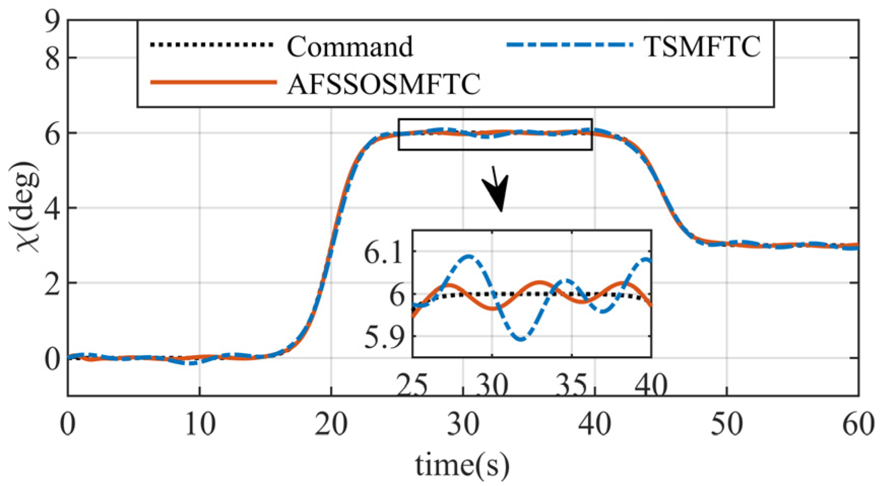
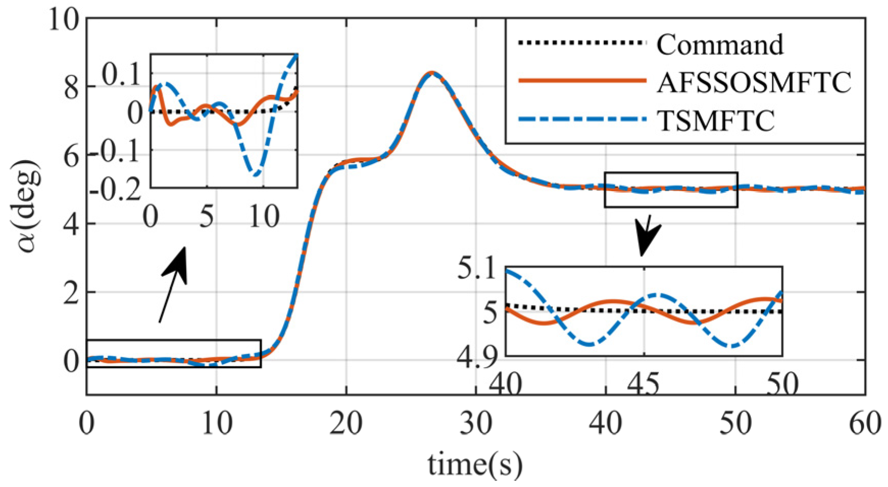
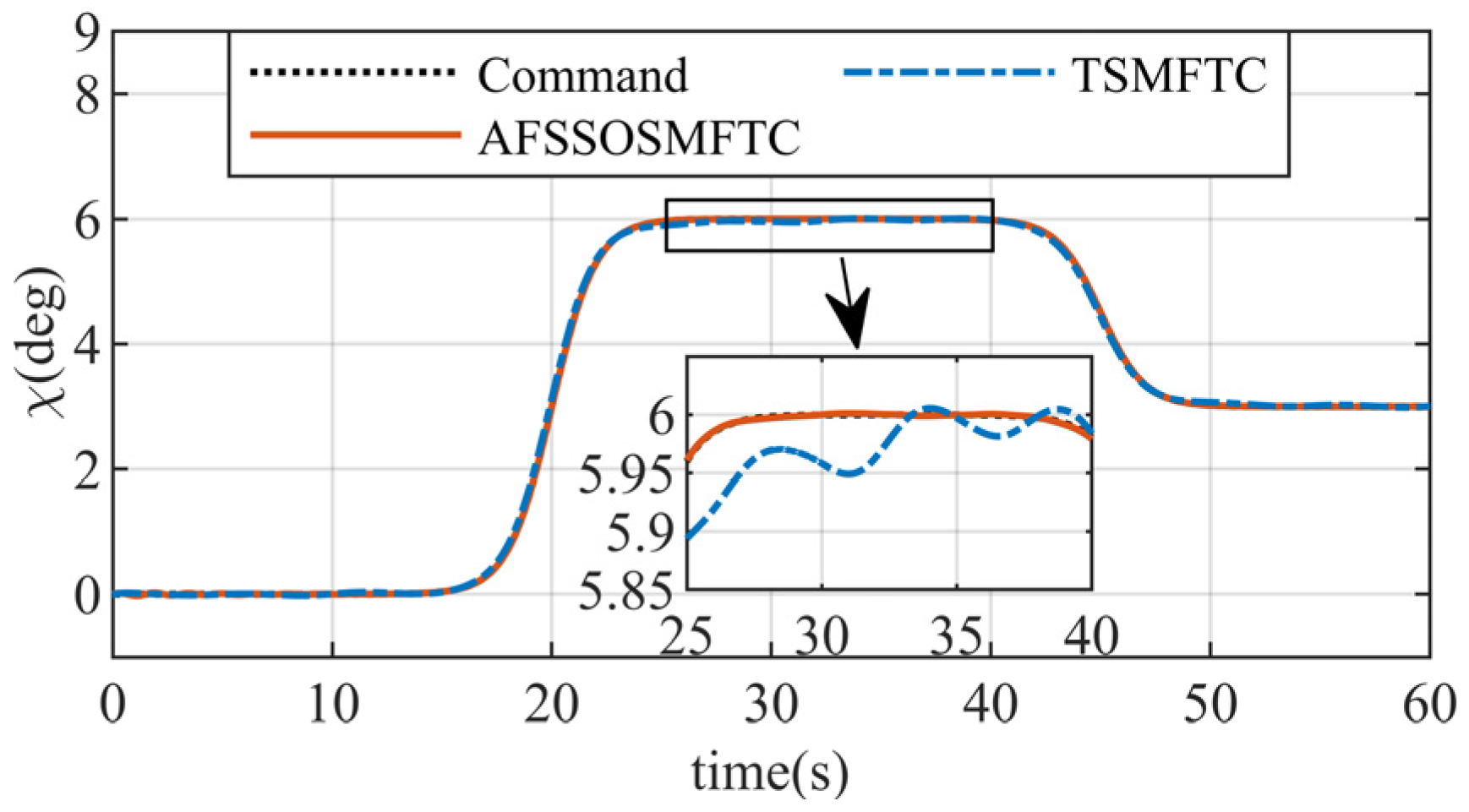
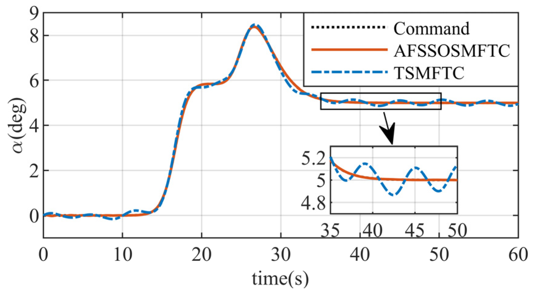
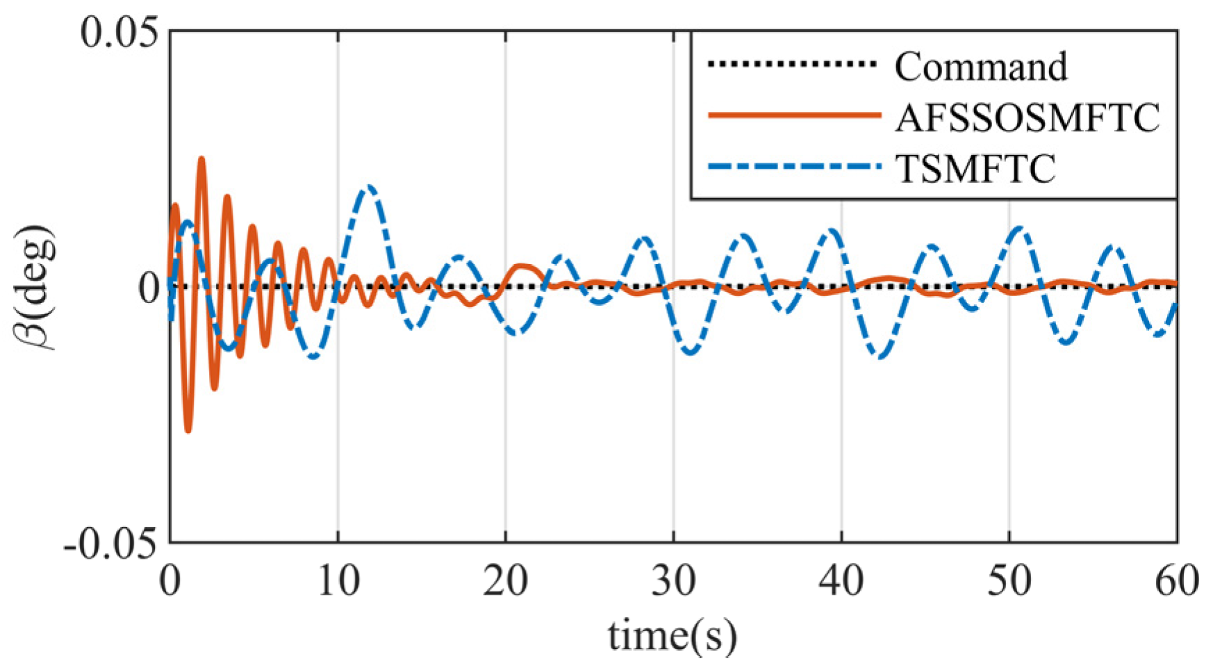
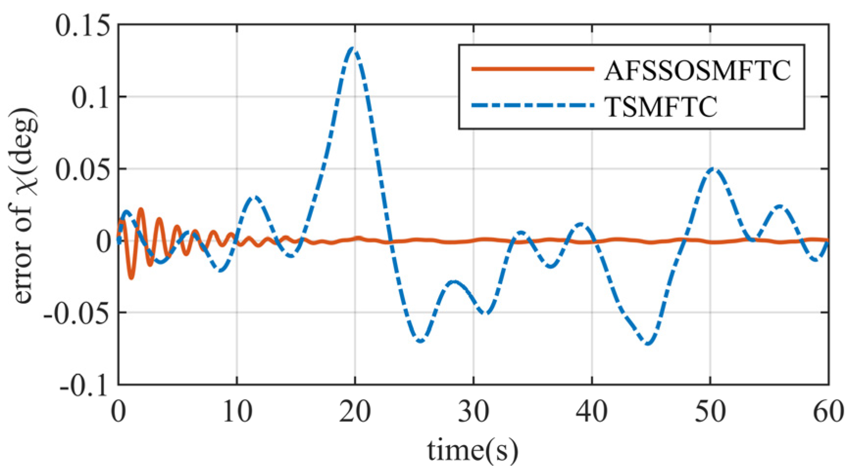
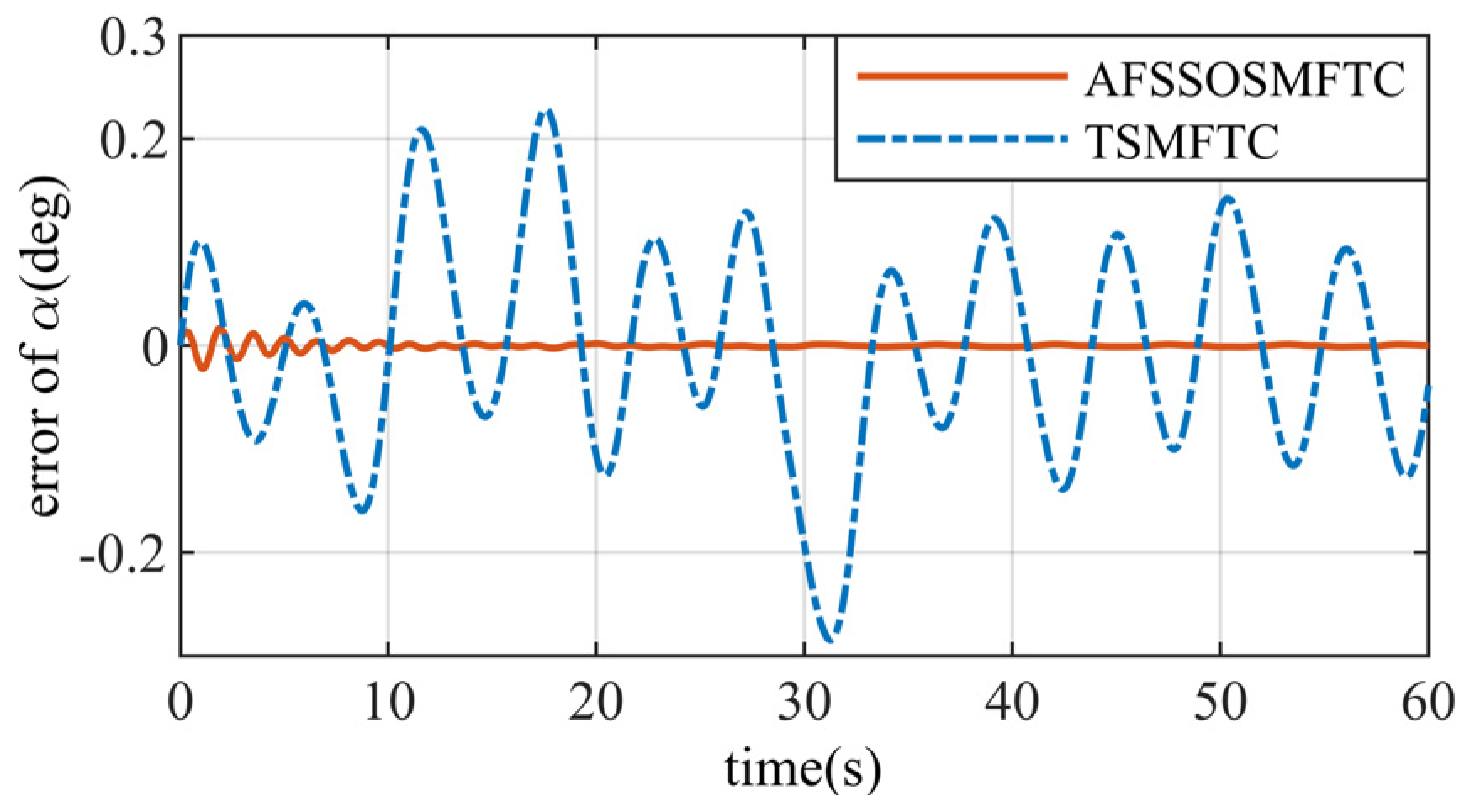
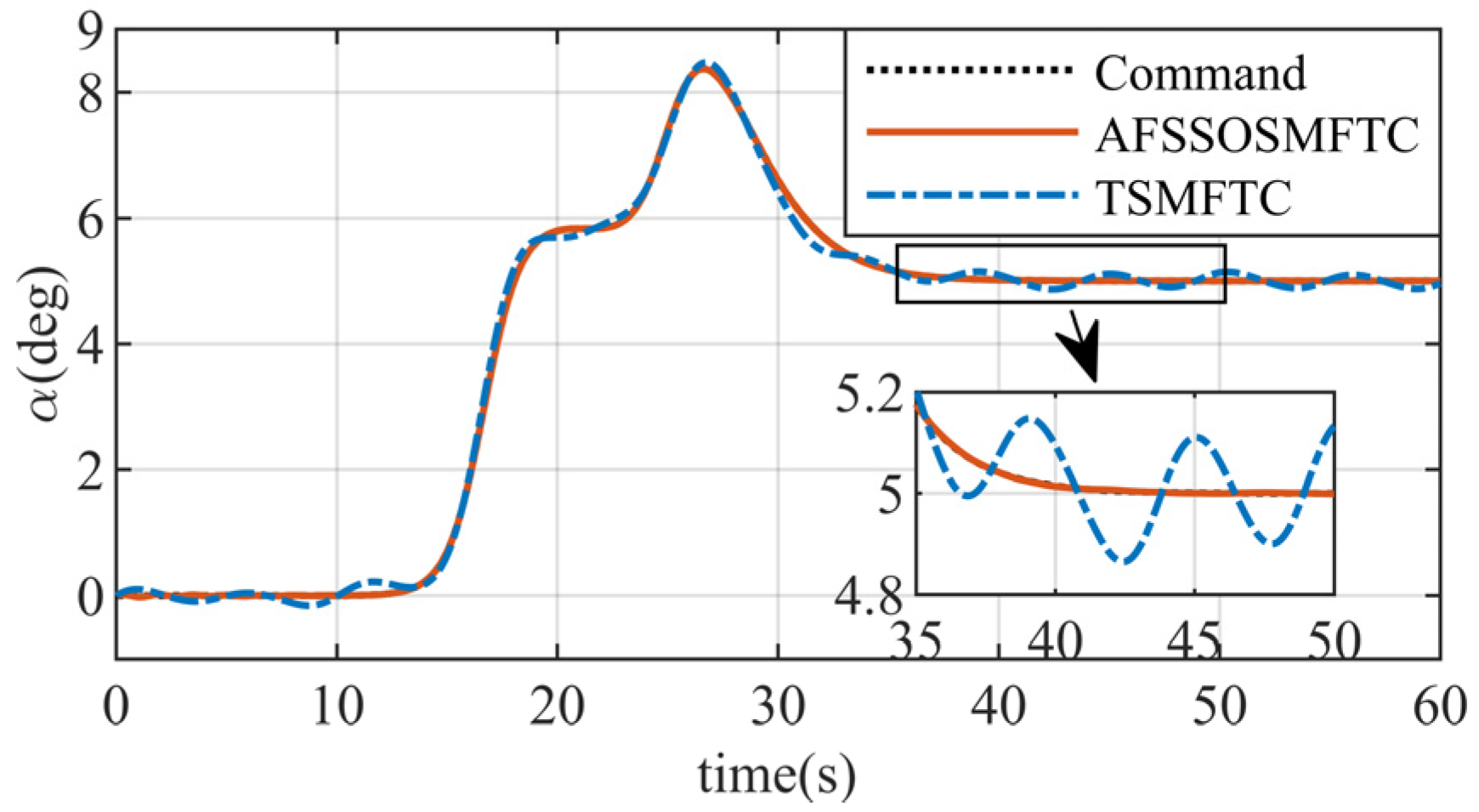
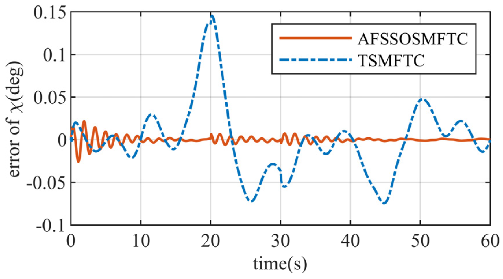
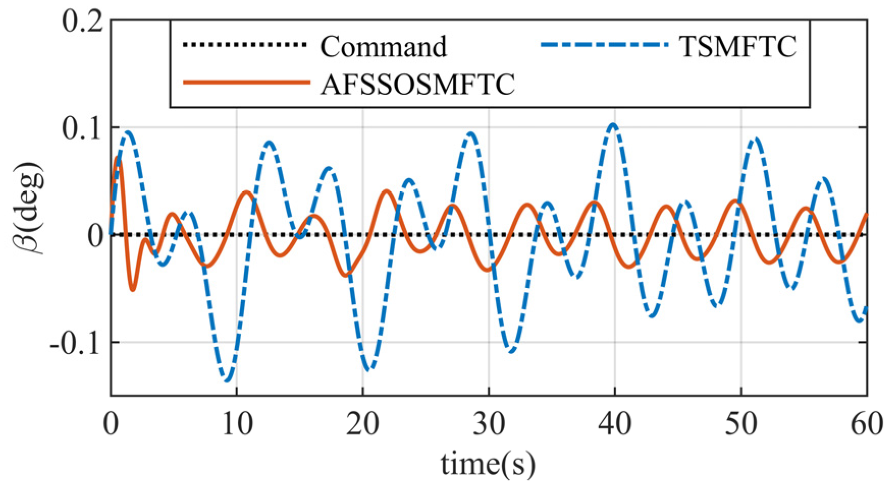
The above figures illustrate the comparison between the AFSSOSMFTC and the terminal sliding mode fault-tolerant controller (TSMFTC). In the presence of disturbances, both methods effectively track the command signal. For roll and pitch angles, the error of the proposed method converges to within $0.04°$, while the maximum error of the TSMFTC exceeds $0.1°$. Since the command for the sideslip angle is $0°$, Figure 5 can simultaneously reflect tracking response and error.

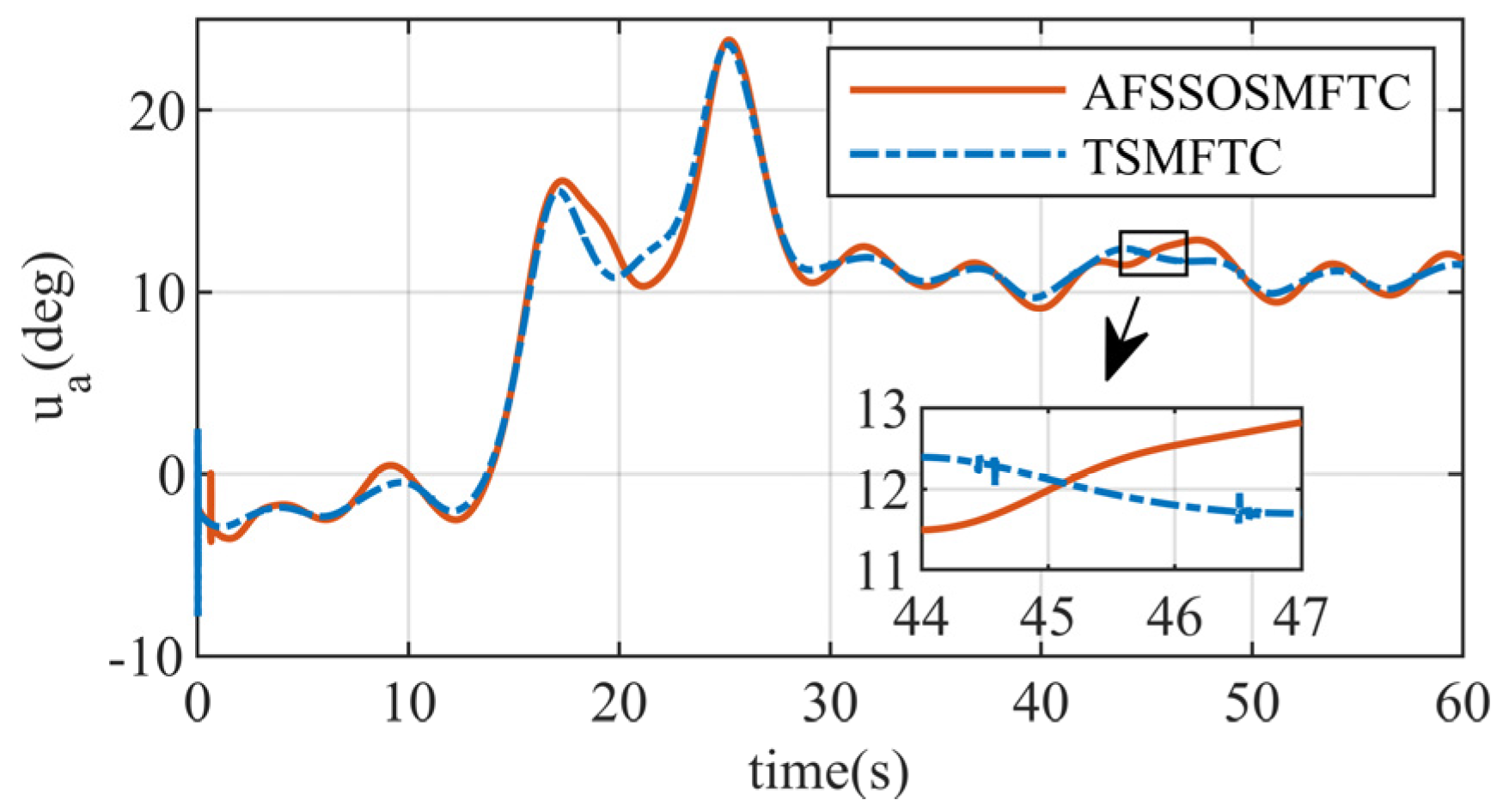
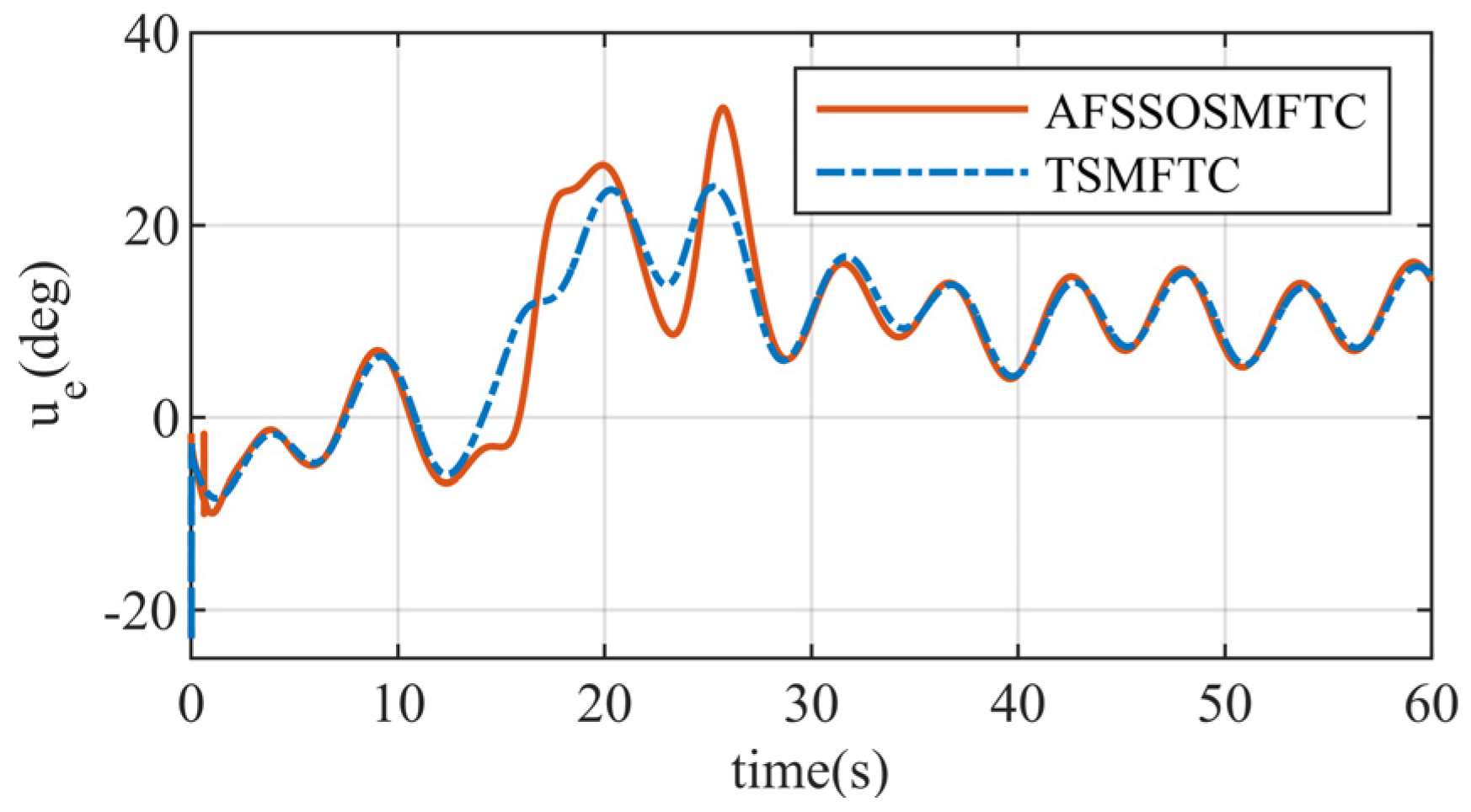
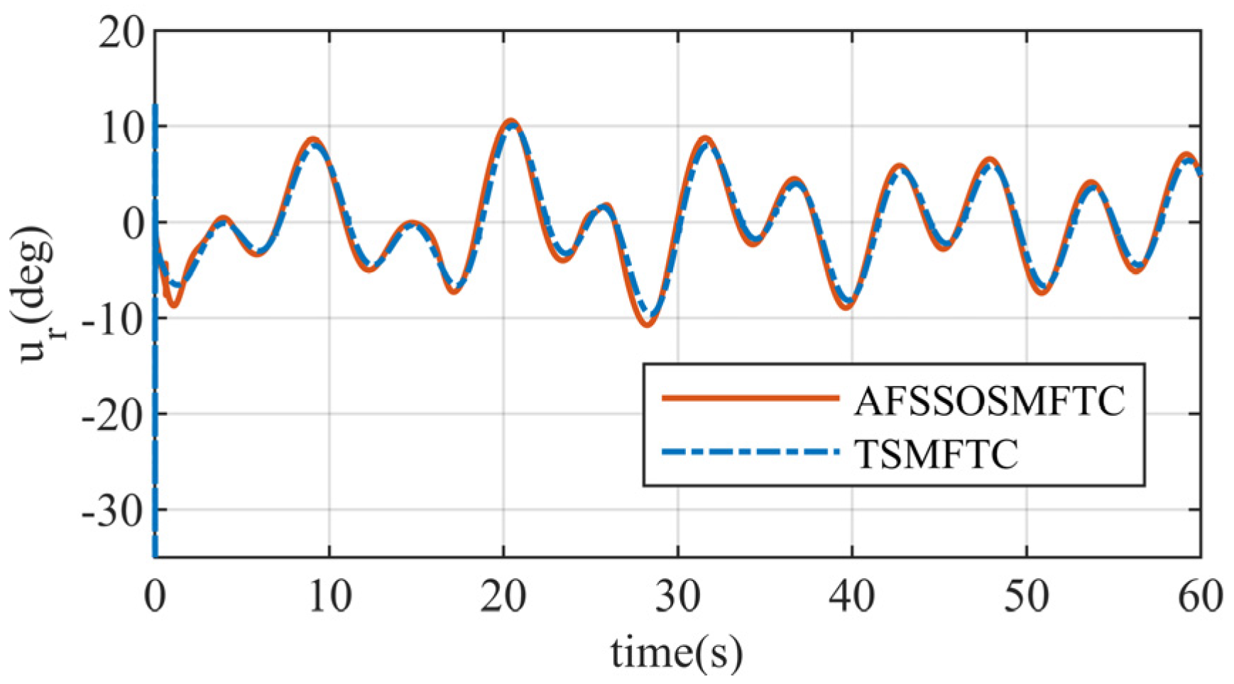
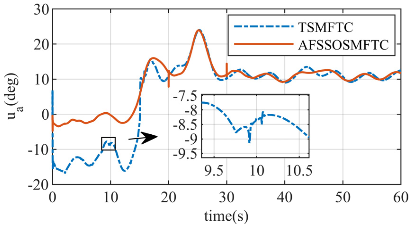
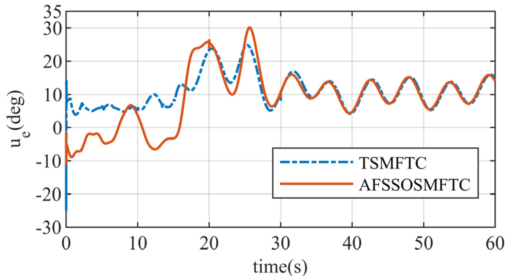
For the control surfaces, the responses of the two methods are similar. Still, the control surface response of the TSMFTC is abrupt at the initial moment, which is not conducive to practical control of the control surfaces. Moreover, small oscillations occur multiple times during the simulation process, as shown in the response in Figure 8. These oscillations are also reflected in the $u_r$ response. The control surface response of the proposed method is smoother and more continuous than that of the TSMFTC. In Figure 9, when the angle of attack command is large, the proposed controller provides more considerable control surface deflections than the TSMFTC. This indicates that the proposed controller is more sensitive to changes in the command.

The results of using the root mean square error method for data analysis are shown in

Table 4. Root mean square error of scenario 1.

Scenario 1	Angle of Bank (deg)	Angle of Attack (deg)	Sideslip Angle (deg)
AFSSOSMFTC	0.02085	0.02055	0.02130
TSMFTC	0.06052	0.06139	0.05795

. Compared to the comparison method, the airflow angle error for the proposed method is reduced by 65.56%, 66.53%, and 63.24%, respectively.

Table 5. The standard deviation of scenario 1.

Scenario 1	Angle of Bank (deg)	Angle of Attack (deg)	Sideslip Angle (deg)
AFSSOSMFTC	0.02084	0.02054	0.02130
TSMFTC	0.06047	0.06131	0.05792

shows the results of the standard deviation analysis. Compared to the comparison method, the airflow angle error for the proposed method is reduced by 65.53%, 66.50%, and 63.23%, respectively.

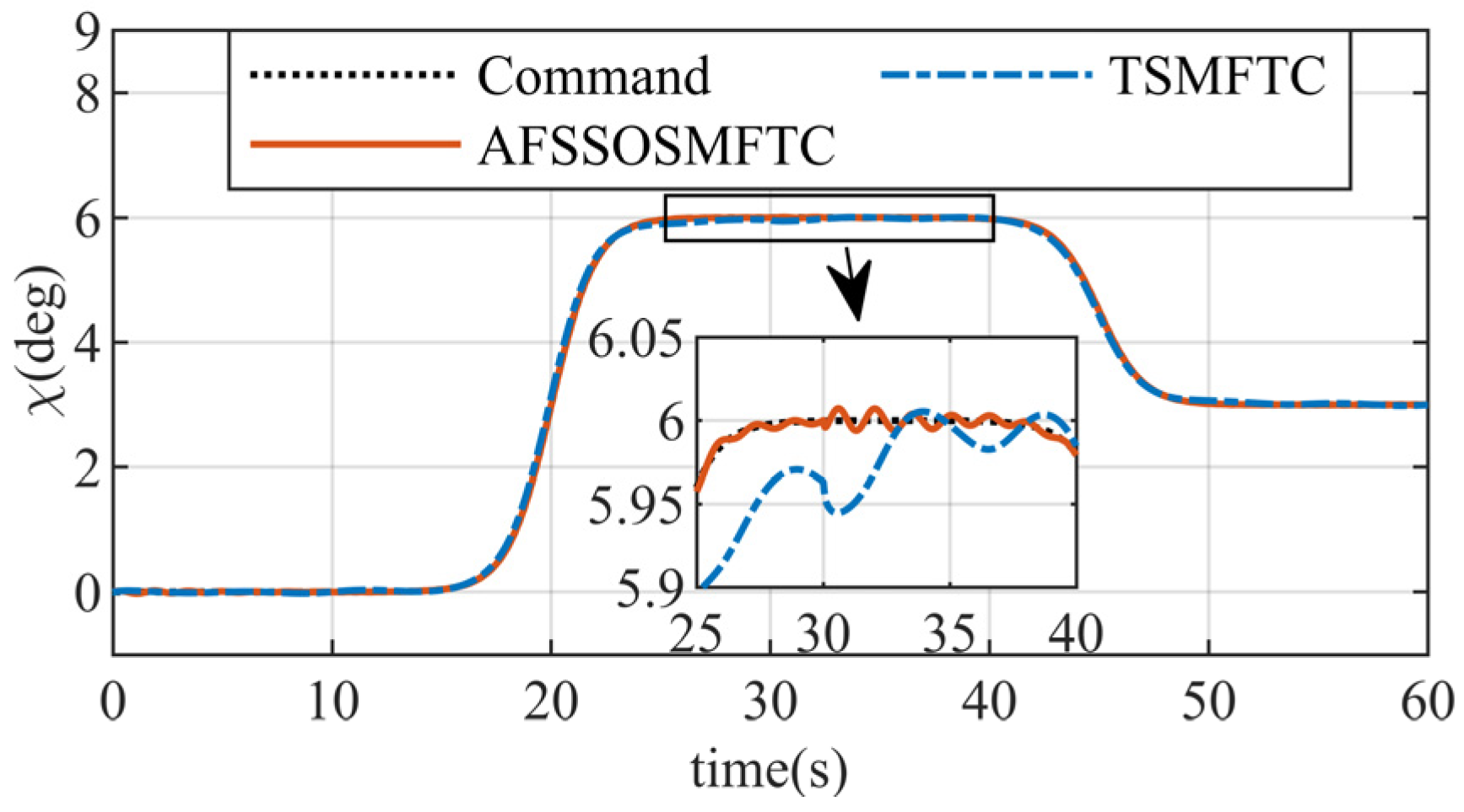
5.2. Scenario 2

The state variable responses and error curves after introducing the disturbance observer are shown in Figure 11, Figure 12, Figure 13, Figure 14, Figure 15, Figure 16, Figure 17 and Figure 18.

After compensating for the aggregated disturbance by introducing the disturbance observer, the control performance of the proposed method is significantly improved. The steady-state error of the airflow angle converges to near $0°$ in a short time, demonstrating rapid convergence. The TSMFTC also performs well in roll and pitch angle responses, with errors mainly within the range of $0.05°$ compared to the uncompensated case. However, there is no significant improvement in the angle of attack response.

In the control surface response, the initial weak oscillations in the proposed method are improved, resulting in a smoother overall response. The terminal sliding mode method exhibits significant high-frequency oscillations around 30 s, and small-scale oscillations persist, showing no significant improvement. This indicates that the proposed controller is more robust.

Table 6. Root mean square error of scenario 2.

Scenario 2	Angle of Bank (deg)	Angle of Attack (deg)	Sideslip Angle (deg)
AFSSOSMFTC	0.00400	0.00329	0.00462
TSMFTC	0.04057	0.10290	0.00742

provides the results of the data analysis. Compared to the comparison method, the airflow angle error for the proposed method is reduced by 90.15%, 96.80%, and 37.82%, respectively. The standard deviation method used in

Table 7. The standard deviation of scenario 2.

Scenario 2	Angle of Bank (deg)	Angle of Attack (deg)	Sideslip Angle (deg)
AFSSOSMFTC	0.00400	0.00329	0.00462
TSMFTC	0.04057	0.10286	0.00742

reflects a reduction of 90.15%, 96.80%, and 37.82% in airflow angle errors, respectively, which is almost consistent with the root mean square error method.

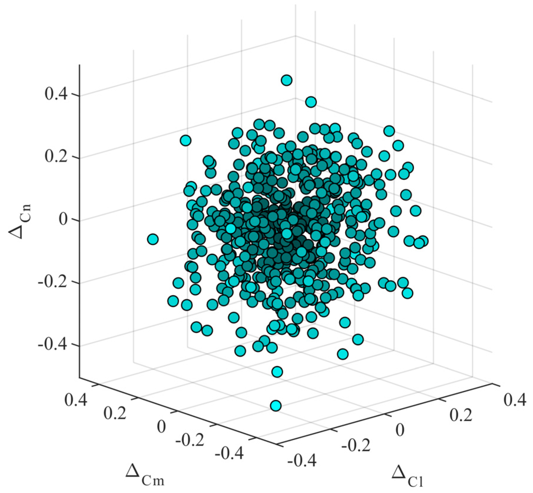
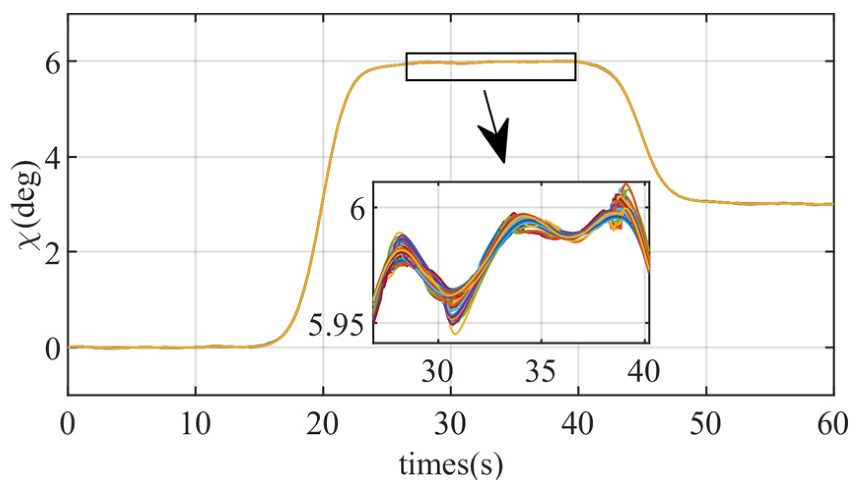
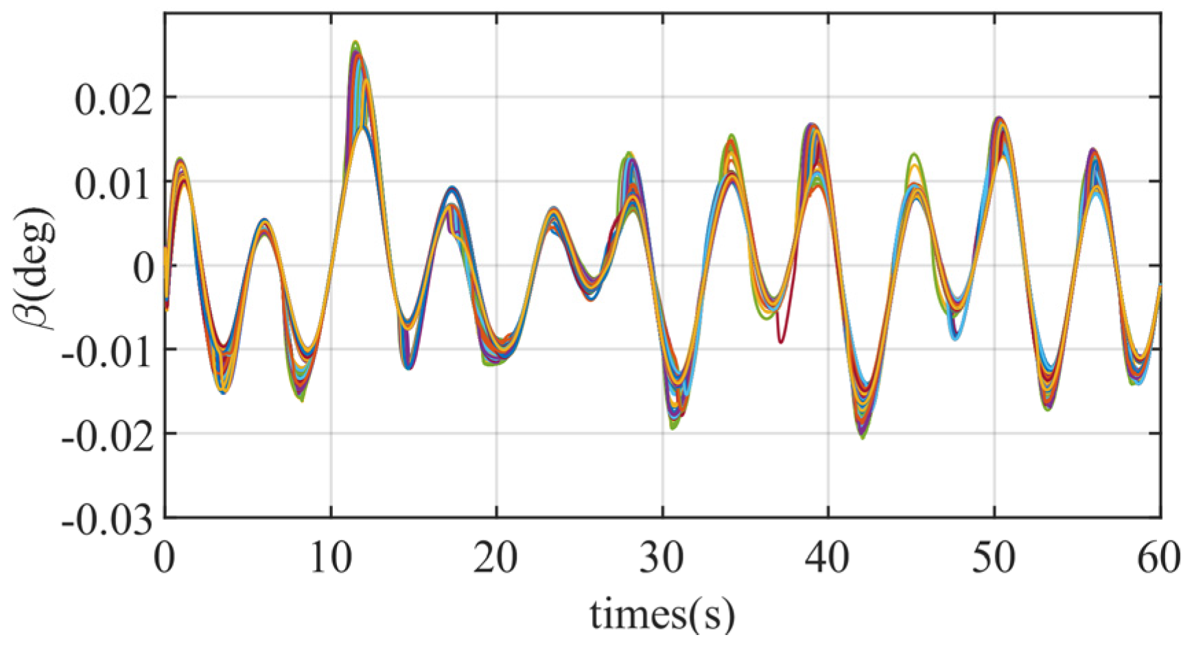
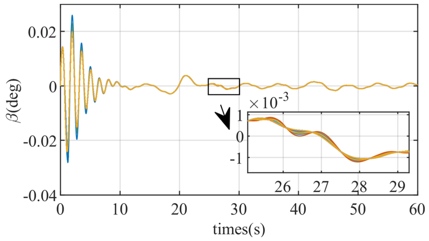
Monte Carlo simulations were performed 500 times, applying deviations to the tri-axial coefficients ${\Delta }_{Cl},{\Delta }_{Cm}$, and ${\Delta }_{Cn}$, each of which follows a normal distribution with a mean of 0 and a standard deviation of 0.15. The deviation scatter plot is shown in Figure 19.

Monte Carlo simulations were conducted for both methods. Figure 20, Figure 21, Figure 22, Figure 23, Figure 24 and Figure 25 present the simulation results of the controller proposed in this paper and the comparison controller. Under the same aerodynamic deviations, both methods demonstrate good control performance. The state variables of the proposed method exhibit almost consistent behavior, with minimal errors across multiple trials. In contrast, the comparative method shows more significant errors in the state variables during repeated simulations, highlighting the stronger robustness of the proposed method against aerodynamic parameter uncertainties.

5.3. Scenario 3

This section considers the presence of control surface faults in the HSV and applies fault compensation. The analysis focuses on the variations in the airflow angle and the response of the control surfaces.

The model for reduced control surface effectiveness in the control surface fault model in Equation (7) is as follows:

$$\kappa =\left\{\begin{array}{cc}0, \hfill & \hfill if t(s)<20\\ {\left[\begin{array}{ccc}0.4& 0.2& 0.1\end{array}\right]}^T,\hfill & \hfill if t(s)\ge 20\end{array}\right.$$

(49)

The model for a control surface slack and floating fault is as follows:

$$u_{c0}=\left\{\begin{array}{cc}0,\hfill & \hfill if t(s)<30\\ \left[\begin{array}{c}5+\sin \left(0.5t\right)\\ 3+\sin \left(0.8t+1.1\right)\\ 5+\sin \left(0.3t+1.8\right)\end{array}\right],\hfill & \hfill if t(s)\ge 30\end{array}\right.$$

(50)

Figure 26, Figure 27, Figure 28, Figure 29, Figure 30, Figure 31, Figure 32 and Figure 33 illustrate the variations in state variables.

After a control surface failure in the HSV, the AFSSOSMFTC and the TSMFTC can converge. The disturbance observer effectively compensates for the control surface fault between 20 and 30 s.

In Figure 26 and Figure 29, it can be observed that after the occurrence of a fault, there is a small oscillation in the airflow angle. The proposed method converges quickly within a short time, while the terminal sliding mode method still exhibits significant errors. However, there is no substantial change in the angle of attack and sideslip angle responses, indicating that the observer compensates well for the control surface fault.

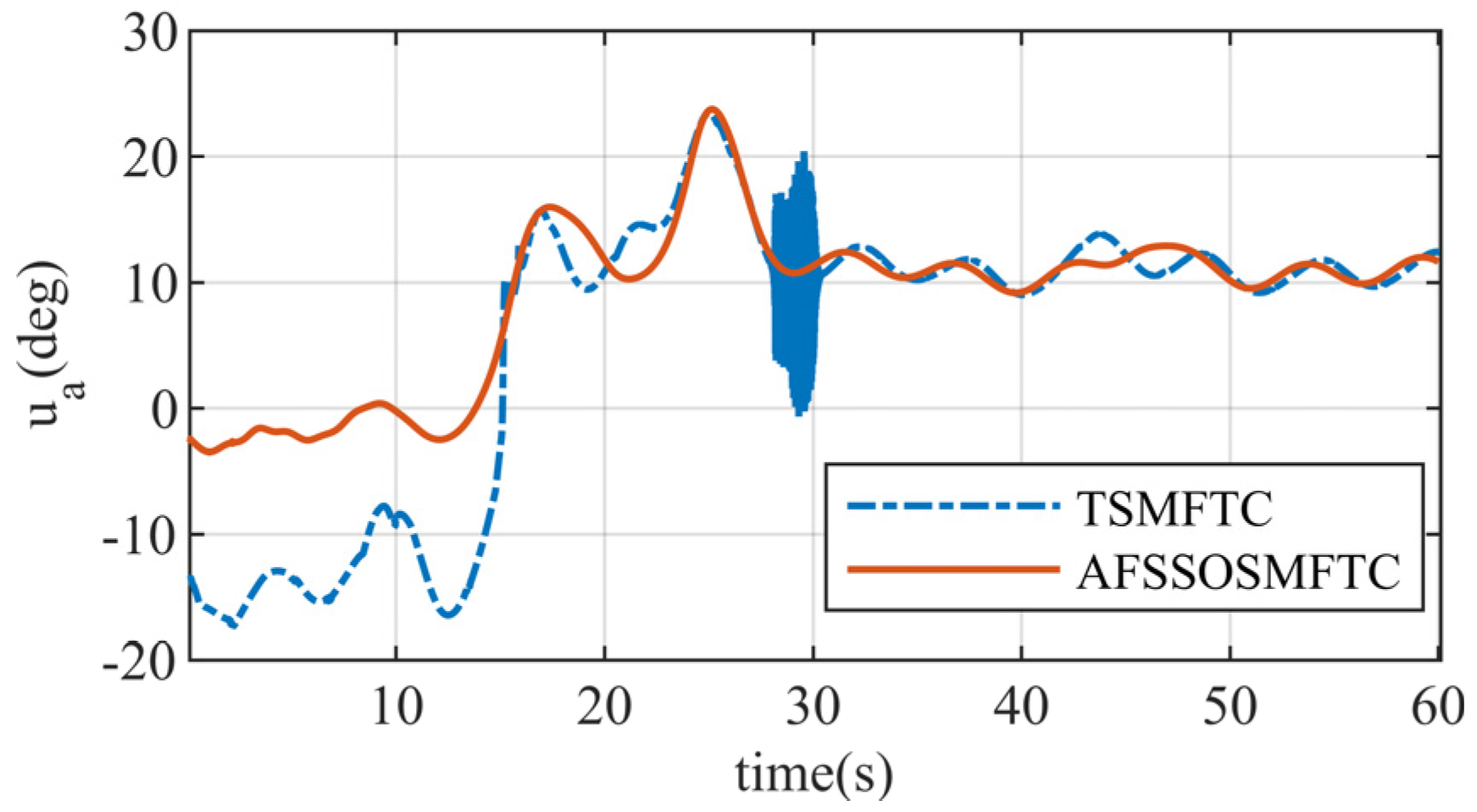
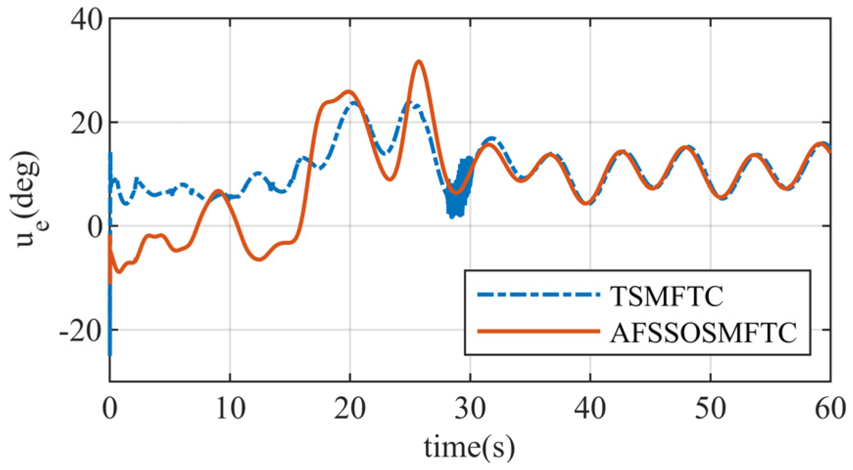
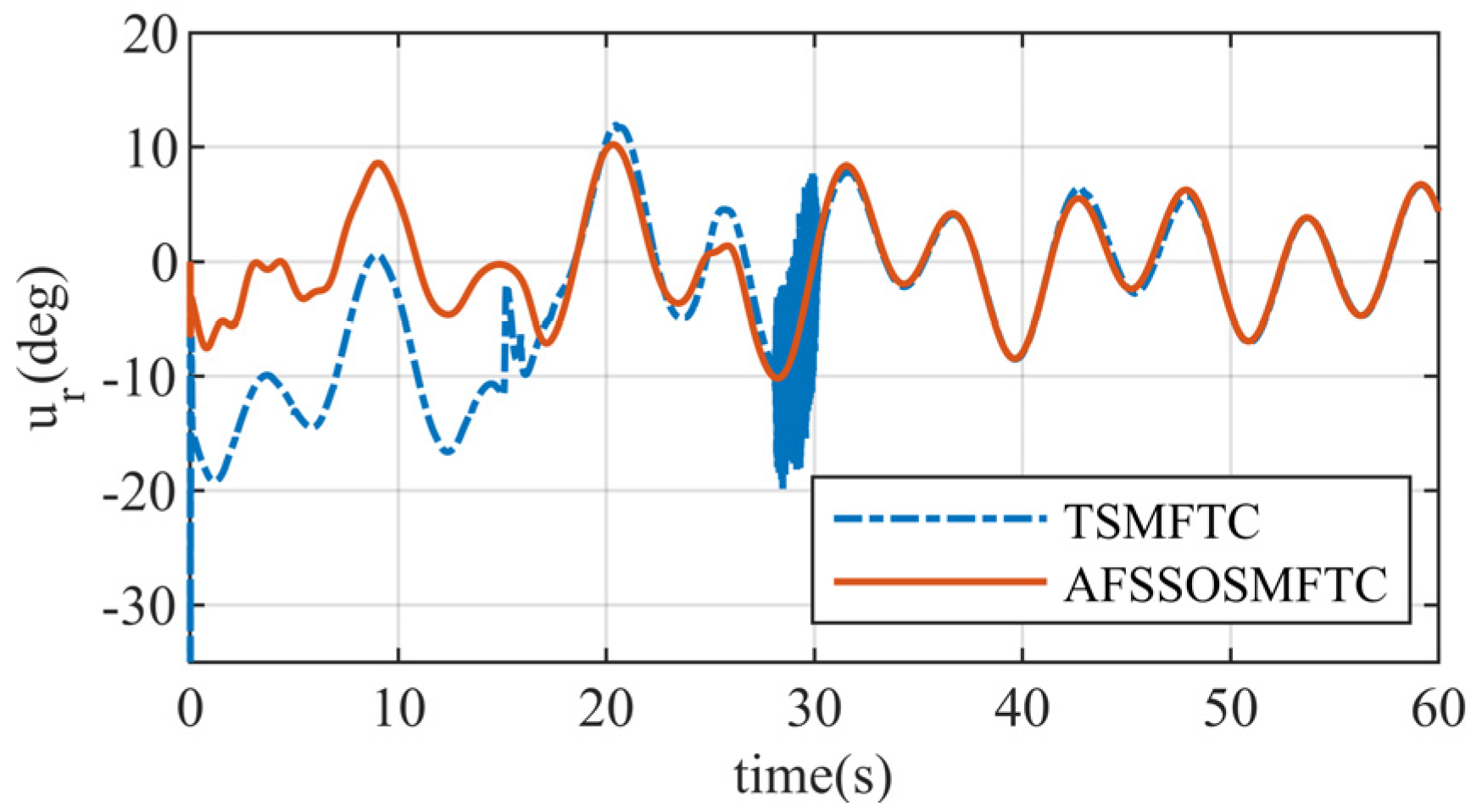
Figure 31, Figure 32 and Figure 33 depict the changes in the control surfaces. Both control methods exhibit control surface oscillations at the initial moment and when the fault occurs. However, the oscillation amplitude of the AFSSOSMFTC is smaller than that of the terminal sliding mode controller. The TSMFTC experiences control surface oscillations at different times, while the proposed controller is smoother and more continuous. It also converges more quickly, validating the advantages of smoothness and speed offered in this paper.

As shown in

Table 8. Root mean square error of scenario 3.

Scenario 3	Angle of Bank (deg)	Angle of Attack (deg)	Sideslip Angle (deg)
AFSSOSMFTC	0.00434	0.00330	0.00462
TSMFTC	0.04201	0.10313	0.00716

, in scenario 3, compared to the comparison method, the airflow angle error for the proposed method is reduced by 89.67%, 96.80%, and 35.47%, respectively.

Table 9. The standard deviation of scenario 3.

Scenario 3	Angle of Bank (deg)	Angle of Attack (deg)	Sideslip Angle (deg)
AFSSOSMFTC	0.00434	0.00330	0.00462
TSMFTC	0.04201	0.10309	0.00716

shows the analysis results of the standard deviation method, where the airflow angle errors were reduced by 89.67%, 97.09%, and 35.47%, respectively, which is almost consistent with the root mean square error method.

6. Conclusions

In this article, an AFSSOSMFTC is proposed. A fixed-time disturbance observer is designed to estimate and compensate for external aggregated disturbances and actuator faults. On this basis, a first-order filter is used to calculate the derivatives, and it is compared with the terminal sliding mode controller. The analysis under three scenarios demonstrates that the proposed controller converges much faster than the terminal sliding mode controller, with an average reduction of at least 50% in errors. No significant chattering was observed, and the output signals were smooth. When considering external disturbances and actuator faults, the airflow angle error of the aircraft quickly converges to a very small value, highlighting the robustness and effectiveness of the proposed controller.

The future work will focus on controller design, considering actuator saturation and state constraints. We will also consider position control issues that are more challenging than attitude control and implement the controller in a semi-physical simulation setup for hardware-in-the-loop testing.