Three-Dimensional Rapid Orbit Transfer of Diffractive Sail with a Littrow Transmission Grating-Propelled Spacecraft

Abstract

A diffractive solar sail is an elegant concept for a propellantless spacecraft propulsion system that uses a large, thin, lightweight surface covered with a metamaterial film to convert solar radiation pressure into a net propulsive acceleration. The latter can be used to perform a typical orbit transfer both in a heliocentric and in a planetocentric mission scenario. In this sense, the diffractive sail, proposed by Swartzlander a few years ago, can be considered a sort of evolution of the more conventional reflective solar sail, which generally uses a metallized film to reflect the incident photons, studied in the scientific literature starting from the pioneering works of Tsander and Tsiolkovsky in the first decades of the last century. In the context of a diffractive sail, the use of a metamaterial film with a Littrow transmission grating allows for the propulsive acceleration magnitude to be reduced to zero (and then, the spacecraft to be inserted in a coasting arc during the transfer) without resorting to a sail attitude that is almost edgewise to the Sun, as in the case of a classical reflective solar sail. The aim of this work is to study the optimal (i.e., the rapid) transfer performance of a spacecraft propelled by a diffractive sail with a Littrow transmission grating (DSLT) in a three-dimensional heliocentric mission scenario, in which the space vehicle transfers between two assigned Keplerian orbits. Accordingly, this paper extends and generalizes the results recently obtained by the author in the context of a simplified, two-dimensional, heliocentric mission scenario. In particular, this work illustrates an analytical model of the thrust vector that can be used to study the performance of a DSLT-based spacecraft in a three-dimensional optimization context. The simplified thrust model is employed to simulate the rapid transfer in a set of heliocentric mission scenarios as a typical interplanetary transfer toward a terrestrial planet and a rendezvous with a periodic comet.

1. Introduction

Thanks to the rapid technological advances in the design and construction of large gossamer space structures [1,2,3,4], in the last two decades the propulsion system based on the solar sail concept has become a viable option [5,6] in the design of space missions both for the study of the Earth [7,8] and for the exploration of the Solar System [9,10,11]. This aspect became evident soon after the successful completion of JAXA’s pioneering deep-space mission named Interplanetary Kite-craft Accelerated by Radiation Of the Sun (IKAROS) [12], which succeeded for the first time in demonstrating the effective capability of deploying (and using) [13,14] a solar sail propulsion system in a heliocentric mission scenario [15]. Indeed, after the IKAROS historical flight, several mission proposals have envisaged the use of a solar sail as the primary propulsion system, as detailed in the interesting reviews by Fu et al. [16], Gong and MacDonald [17], and Spencer et al. [18]. In this context, NASA’s missions as the ill-fated Near-Earth Asteroid Scout [19,20,21] (failed due to a problem during deployment from the Artemis 1 on November 2022) and the Advanced Composite Solar Sail System [22] (launched at the end of April 2024 and currently still active) demonstrate the potential of the solar sail concept also in the design of missions involving small satellites such as CubeSats [23].

A classic solar sail uses a large membrane covered with a (highly reflective) metallized film to substantially reflect the Sun’s rays in such a way as to tend as close as possible to an (ideal) condition of complete and specular reflection [24,25]. However, over the years alternative techniques have been proposed to obtain a net space thrust from solar radiation pressure, using a highly engineered membrane film capable of providing specific (physical) characteristics. In this context, two interesting examples are provided by the refractive sail proposed by Firuzi et al. [26,27] about five years ago, and by the diffractive sail proposed by Swartzlander a few years earlier [28,29,30]. The performances of both these solar sail concepts have been analyzed, in recent years, from the point of view of the preliminary mission design [31,32,33,34,35]. The results obtained indicate that the flight performances of the refractive and diffractive sails are such as to make them a valid alternative (at least from the point of view of numerical simulations) to the more conventional reflective solar sail [36,37].

Starting from the mathematical model discussed in Swartzlander’s seminal paper [28] published in 2017, very recently the author of [38] studied the performance of a special type of diffractive sail, namely a (diffractive) solar sail in which the membrane film obeys diffraction from a grating under the Littrow condition for transmission [39]. In particular, Ref. [38] analyzed the heliocentric orbit transfer performance of a spacecraft propelled by a diffractive sail with a Littrow transmission grating (DSLT) considering a two-dimensional mission scenario, where the thrust vector induced by the sail belongs to the plane of the initial (parking) orbit of the spacecraft throughout the flight. That specific choice of considering a purely two-dimensional transfer made it possible to simplify both the mathematical model of the thrust vector and the study of the (optimal) steering law to be employed in the orbital transfer, since this law involves a single (dimensionless) control parameter, i.e., the so-called sail pitch angle [38]. The latter is defined as the angle between the Sun–spacecraft line and the direction of the unit vector normal to the shadowed side of the sail nominal plane.

The aim of this work is to extend and complete the analysis proposed in Ref. [38] by considering a DSLT-propelled spacecraft in a three-dimensional, heliocentric mission scenario. In particular, starting from the mathematical model discussed in [38] which, in turn, originates from the model proposed by Swartzlander [28], this paper proposes a three-dimensional (simplified) form of the DSLT-induced thrust vector model that can be used to simulate the orbital transfer of the spacecraft in a typical, deep space, preliminary mission design. The three-dimensional thrust model, which has two dimensionless control parameters of which one is essentially the pitch angle, as discussed in Section 2, is employed in this paper to study the rapid transfer trajectories in a heliocentric mission scenario involving two Keplerian orbits of assigned characteristics. More specifically, this work studies a classical interplanetary transfer between the heliocentric orbit of the Earth and that of one of the remaining terrestrial planets, or that of the periodic comet 29P/Schwassmann–Wachmann [40]. The results of numerical simulations are detailed in Section 3. Finally, Section 4 summarizes the conclusion of the work.

2. Mathematical Preliminaries and Solar Sail Thrust Model

This section illustrates the mathematical model used to evaluate the transfer performance of the DSLT-propelled spacecraft in the three-dimensional (heliocentric) mission scenarios illustrated later in the paper. In particular, this section first describes the sail thrust model starting from the results of the literature [28,38], and then briefly illustrates (without going into detail since it has already been widely discussed in the author’s recent literature both for a reflective [41] and a diffractive sail [34]) the mathematical model used for the optimization of the transfer trajectory from the point of view of the total flight time.

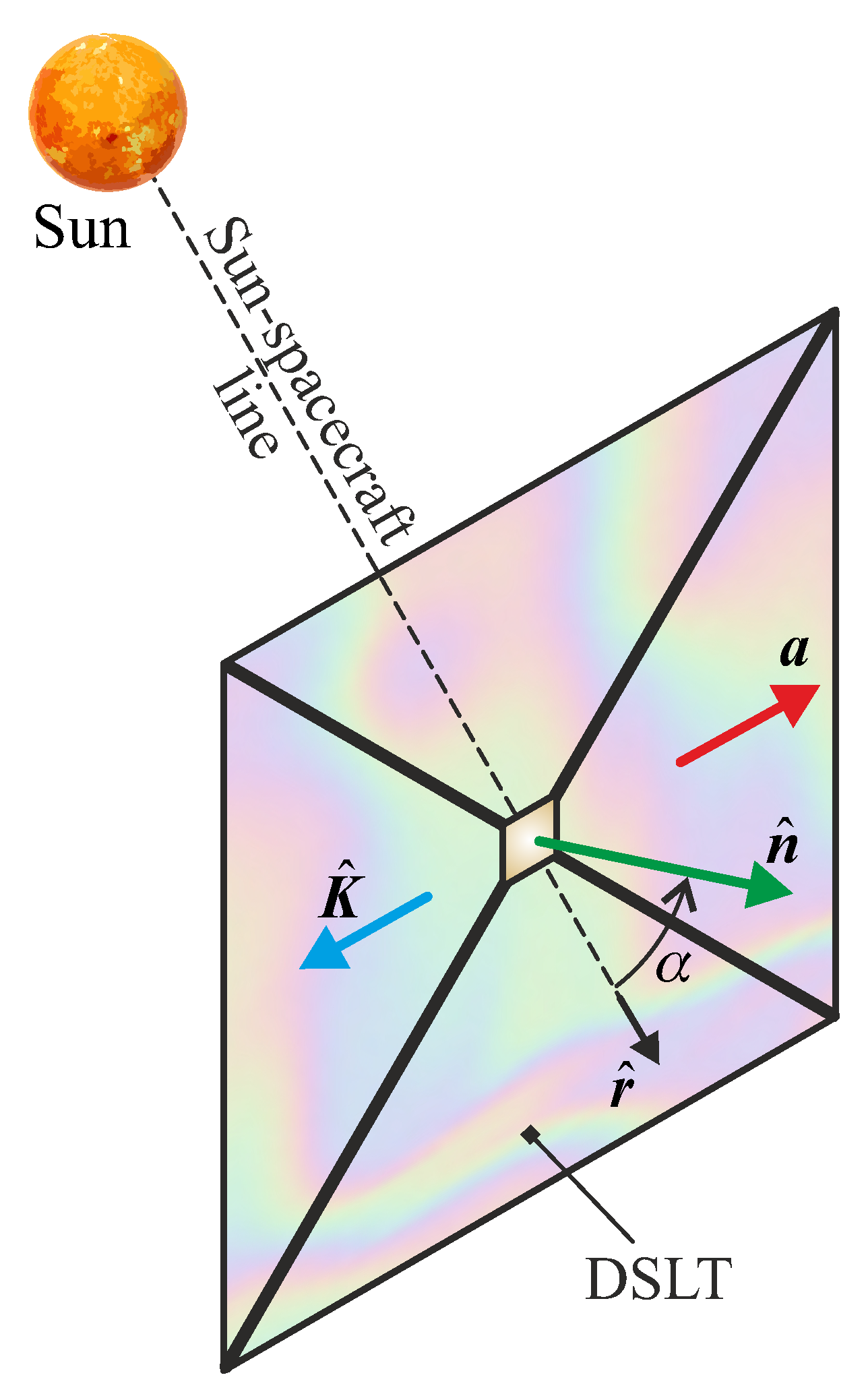
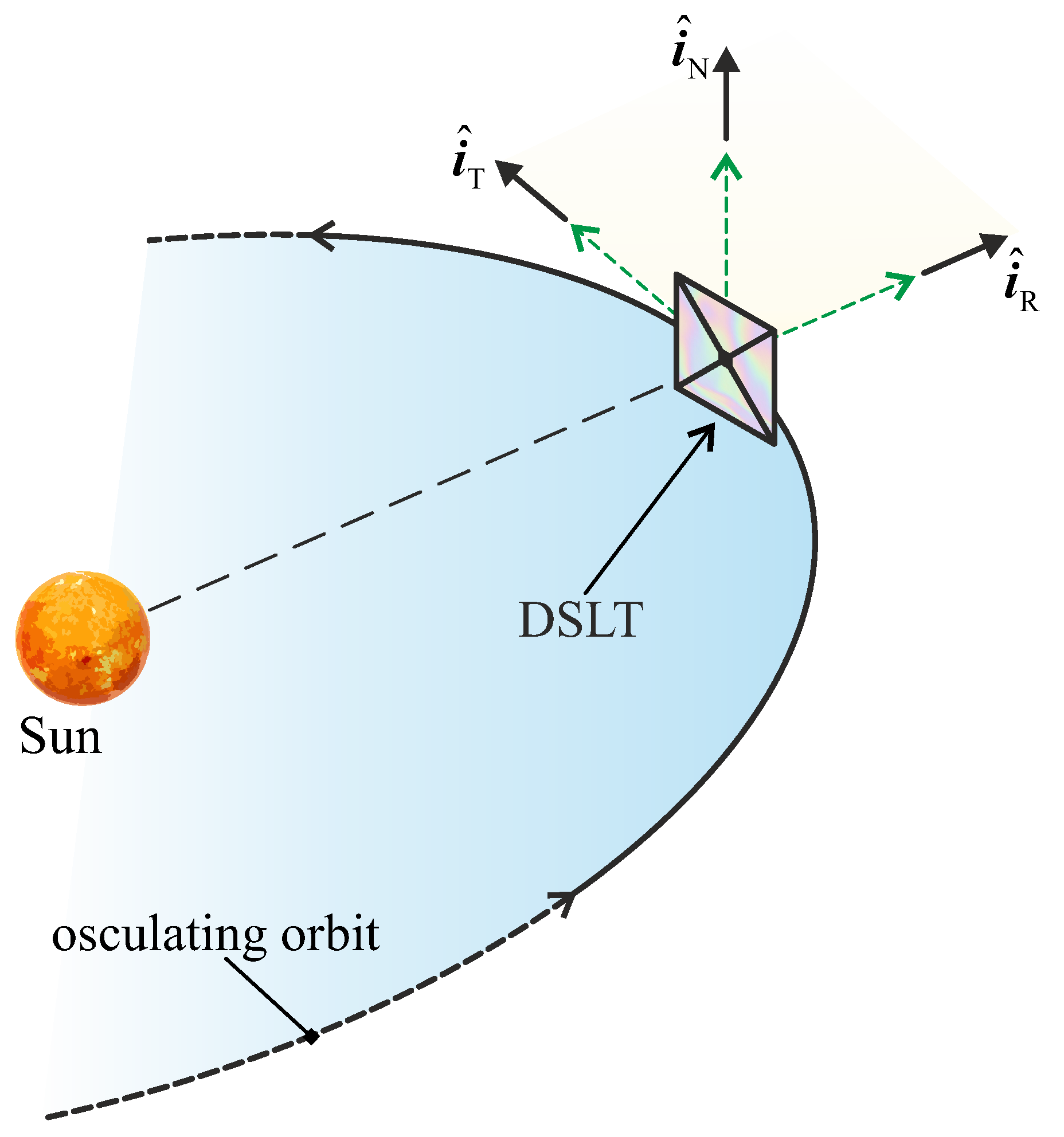
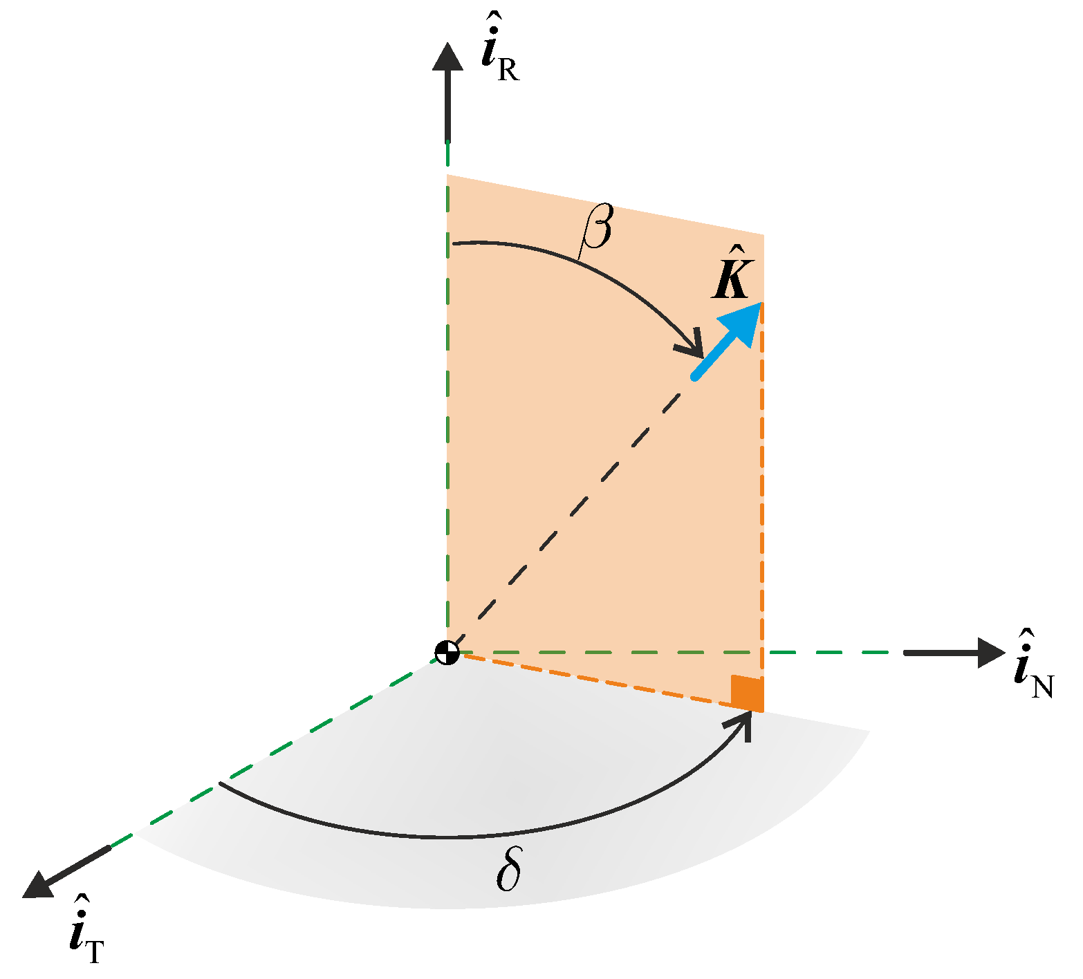
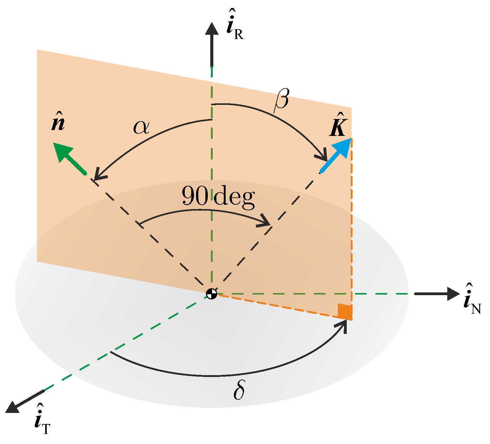
2.1. Simplified DSLT Thrust Model in a Three-Dimensional Heliocentric Scenario

Considering a spacecraft with a DSLT-based propulsion system, the starting point for writing a simplified thrust model useful for the preliminary study of the space vehicle’s transfer trajectory through the solution of a classical optimal control problem, is constituted by Equation (9) obtained by Swartzlander in Ref. [28]. In particular, that equation relates the local value of the propulsive acceleration vector $\mathit{a}$ to the Sun–spacecraft unit vector $\widehat{\mathit{r}}$, the grating momentum unit vector $\widehat{\mathit{K}}$ as defined in Ref. [31], and the angle $\alpha \in [0,90]\mathrm{deg}$ between the Sun–spacecraft line and the direction of the unit vector $\widehat{\mathit{n}}$ normal to the sail nominal plane (side opposite to the Sun). In this respect, a sketch of the DSLT geometry with terms $\alpha$, $\widehat{\mathit{n}}$, $\widehat{\mathit{r}}$, $\mathit{a}$, and $\widehat{\mathit{K}}$ is shown in Figure 1.

Note that, according to the typical nomenclature related to the study of solar sails [24,25], in a three-dimensional thrust model the angle $\alpha$ is usually referred to as the “cone angle”, while in a two-dimensional thrust model $\alpha$ is the pitch angle, as discussed in the previous section. In particular, Equation (9) of Ref. [28] has been recently rewritten by the author of [38] in a form more useful for the study of the optimal control law in an interplanetary transfer trajectory. In this case, the results are summarized by Equations (1) and (2) of Ref. [38], which give a compact vector expression of the propulsive acceleration $\mathit{a}$, viz.

$$\mathit{a}=-a_c{\left({\displaystyle \frac{r_{\oplus }}{r}}\right)}^{2}sin\left(2\alpha \right)\widehat{\mathit{K}}$$

(1)

where r is the Sun–spacecraft (radial) distance, $r_{\oplus }\triangleq 1\mathrm{AU}$ is a reference distance, and $a_c>0$ is the spacecraft characteristic acceleration. The latter is the typical (scalar) performance parameter in solar sail design and is defined as the maximum value of $\parallel \mathit{a}\parallel$ when the spacecraft’s distance from the Sun is equal to 1 astronomical unit, i.e., when $r=r_{\oplus }$. Recall that, as discussed in Ref. [38], a diffractive sail and a reflective sail with the same value of sail loading [24] (i.e., the same value of the mass-to-area ratio) have a characteristic acceleration in a ratio of 1 to 2. In particular, according to Equation (1), at a given solar distance r the maximum value of the propulsive acceleration magnitude is reached when the cone angle is $\alpha =45\mathrm{deg}$, while a zero value of $\parallel \mathit{a}\parallel$ can be obtained when $\alpha =90\mathrm{deg}$ or $\alpha =0\mathrm{deg}$. The latter condition, that is, the possibility to reduce to zero the propulsive acceleration magnitude with a substantially Sun-facing attitude in which the sail nominal plane is perpendicular to the Sun-spacecraft line, is an interesting (peculiar) characteristic of the DSLT. In fact, in an ideal (flat) reflective sail, the condition $\parallel \mathit{a}\parallel =0$ is obtained only with a sail cone angle close to $90\mathrm{deg}$, that is, with an edgewise attitude with respect to the Sun. The latter is usually a complex configuration to obtain from the point of view of the attitude control implementation. On the other hand, in a DSLT-propelled spacecraft the condition $\parallel \mathit{a}\parallel =0$, which allows for the space vehicle to be inserted in a coasting arc during the heliocentric flight, can be obtained with a small value of the sail cone angle, that is, with an attitude that can be even reached passively through a suitable design of the sail structure, as pointed out by McInnes [42].

Equation (1) can be used to obtain a simplified thrust model of a DSLT-propelled spacecraft, which can be used in a general, three-dimensional, heliocentric mission scenario. To this end, introduce a typical Radial–Transverse–Normal (RTN) reference frame of unit vectors ${\widehat{\mathit{i}}}_{\mathrm{R}}$, ${\widehat{\mathit{i}}}_{\mathrm{T}}$, and ${\widehat{\mathit{i}}}_{\mathrm{N}}$. The RTN frame is sketched in Figure 2, in which ${\widehat{\mathit{i}}}_{\mathrm{R}}$ is directed along the Sun–spacecraft line, $({\widehat{\mathit{i}}}_{\mathrm{T}},{\widehat{\mathit{i}}}_{\mathrm{N}})$ coincides with the plane of the spacecraft osculating orbit, and ${\widehat{\mathit{i}}}_{\mathrm{T}}$ directed along the inertial spacecraft velocity vector.

Keeping in mind that the direction of $\mathit{a}$ is opposite to that of $\widehat{\mathit{K}}$, as seen in Equation (1) and the scheme of Figure 1, and remembering that the solar sail cannot provide a thrust vector directed toward the Sun, in the RTN reference frame the unit vector of grating momentum $\widehat{\mathit{K}}$ can be described through the two angles $\beta \in [90,180]\mathrm{deg}$ and $\delta \in [0,360]\mathrm{deg}$ defined in Figure 3.

Accordingly, one obtains the expression of the unit vector of grating momentum $\widehat{\mathit{K}}$ as

$$\widehat{\mathit{K}}=cos\beta {\widehat{\mathit{i}}}_{\mathrm{R}}+sin\beta cos\delta {\widehat{\mathit{i}}}_{\mathrm{T}}+sin\beta sin\delta {\widehat{\mathit{i}}}_{\mathrm{N}}$$

(2)

To simplify both the mathematical description of the sail thrust vector and the design of the attitude control system we assume that, for a given pair of angles $\{\beta ,\delta \}$, the value of the sail cone angle $\alpha$ has the minimum admissible value. In other words, for a given configuration of the unit vector $\widehat{\mathit{K}}$ in the RTN reference frame, we assume a value of the cone angle close to that which can be passively maintained by an appropriate design of the sail structure. This specific hypothesis corresponds to considering the three unit vectors $\widehat{\mathit{n}}$, $\widehat{\mathit{K}}$ and ${\widehat{\mathit{i}}}_{\mathrm{R}}$ as belonging to the same plane, which coincides with the orange plane drawn in Figure 3 and Figure 4.

Therefore, according to the scheme sketched in Figure 4, and keeping in mind that $\widehat{\mathit{K}}·\widehat{\mathit{n}}=0$ with $\alpha \in [0,90]\mathrm{deg}$, the expression of the cone angle that will be assumed in the rest of the paper is

$$\alpha =\beta -\pi /2\mathrm{rad}$$

(3)

Note that a more general expression of the sail cone angle can be obtained by considering a generic DSLT attitude in the RTN reference frame. However, in that case the cone angle $\alpha$ would be a function of two (scalar) parameters while the direction of the propulsive acceleration vector would depend on three scalar parameters corresponding to the three classical Euler angles that define the orientation of a DSLT body reference system with respect to the RTN orbital frame. This interesting aspect, which further extends the thrust model discussed in this paper, is left to future work.

Using Equations (2) and (3) to write $\widehat{\mathit{K}}$ and $\alpha$, respectively, and bearing in mind the general expression of $\mathit{a}$ given by Equation (1), the radial ($a_{\mathrm{R}}$), transverse ($a_{\mathrm{T}}$), and normal ($a_{\mathrm{N}}$) components of the propulsive acceleration vector are obtained as

$$\begin{array}{cc}\hfill a_{\mathrm{R}}\triangleq \mathit{a}·{\widehat{\mathit{i}}}_{\mathrm{R}}& =a_c{\left({\displaystyle \frac{r_{\oplus }}{r}}\right)}^{2}sin\left(2\beta \right)cos\beta \hfill \end{array}$$

(4)

$$\begin{array}{cc}\hfill a_{\mathrm{T}}\triangleq \mathit{a}·{\widehat{\mathit{i}}}_{\mathrm{T}}& =a_c{\left({\displaystyle \frac{r_{\oplus }}{r}}\right)}^{2}sin\left(2\beta \right)sin\beta cos\delta \hfill \end{array}$$

(5)

$$\begin{array}{cc}\hfill a_{\mathrm{N}}\triangleq \mathit{a}·{\widehat{\mathit{i}}}_{\mathrm{N}}& =a_c{\left({\displaystyle \frac{r_{\oplus }}{r}}\right)}^{2}sin\left(2\beta \right)sin\beta sin\delta \hfill \end{array}$$

(6)

in which one observe that the two scalar control parameters are the two angles $\beta$ and $\delta$. Moreover, it is interesting to note that Equations (4) and (5) are consistent with the results obtained in Ref. [38] for a two-dimensional heliocentric mission scenario. In fact, when $\delta =0\mathrm{rad}$ (i.e., in a two-dimensional case in which the spacecraft moves into the plane defined by the unit vectors ${\widehat{\mathit{i}}}_{\mathrm{R}}$ and ${\widehat{\mathit{i}}}_{\mathrm{T}}$) and the angle $\beta$ is written as a function of $\alpha$ through Equation (3), one obtains that Equations (4) and (5) reduce to Equations (5) and (6) of Ref. [38].

Finally, the Equations (4)–(6) can be used to draw the force bubble of the DSLT thrust vector, that is, the surface on which the tip of the propulsive acceleration vector $\mathit{a}$ lies when the two angles $\beta$ and $\delta$ vary within their admissible ranges [43]. In this case, the DSLT-based force bubble is shown in the left part of Figure 5, while the right part of the figure draws the section of the force bubble with a plane containing the Sun–spacecraft (radial) line. Note as the right part of Figure 5 is consistent with the graph reported in Figure 3 of Ref. [38].

Note that the force bubble of a DSLT-propelled spacecraft is significantly different from that obtained by considering a classical reflective solar sail, which has been reported for comparison purposes in Figure 6. In fact, a reflective solar sail reaches the maximum magnitude of the propulsive acceleration vector when the nominal plane is substantially perpendicular to the Sun–spacecraft line.

2.2. DSLT-Propelled Spacecraft Dynamics

The expression of the three components $\{a_{\mathrm{R}},a_{\mathrm{T}},a_{\mathrm{N}}\}$ of the propulsive acceleration vector given by Equations (4)–(6) are used to write the equations of motion of a DSLT-propelled spacecraft in the heliocentric space. To this end, the vehicle’s dynamics is expressed in terms of the six modified equinoctial orbital elements (MEOE’s) $\{p,f,g,h,k,L\}$ introduced and illustrated in Ref. [44]. The expressions of the MEOEs as a function of the classical orbital elements of the spacecraft osculating orbit are

$$\begin{array}{c}p=a\left(1-e^2\right),f=ecos(\omega +\Omega ),g=esin(\omega +\Omega ),h=tan(i/2)cos\Omega ,\hfill \\ \hfill k=tan(i/2)sin\Omega ,L=\nu +\Omega +\omega \end{array}$$

(7)

where a is the semimajor axis, e is the eccentricity, i is the orbital inclination, $\omega$ is the argument of perihelion, $\Omega$ is the right ascension of the ascending node, and $\nu$ is the true anomaly of the DSLT-propelled spacecraft.

The spacecraft equations of motion are written by recurring to the elegant (vectorial) approach used by Betts in Ref. [45]. The result is the mathematical model summarized by Equations (9)–(12) of Ref. [41], which is just reported below for the sake of completeness

$$\dot{\mathit{x}}=\mathbb{A}{\left[\begin{array}{ccc}{a}_{\mathrm{R}}& a_{\mathrm{T}}& a_{\mathrm{N}}\end{array}\right]}^{\mathrm{T}}+{\left[\begin{array}{cccccc}0& 0& 0& 0& 0& \sqrt{{\mu }_{\odot }p}{\left({\displaystyle \frac{1+fcosL+gsinL}{p}}\right)}^2\end{array}\right]}^{\mathrm{T}}$$

(8)

where ${\mu }_{\odot }$ is the Sun’s gravitational parameter, $\mathit{x}$ is the spacecraft state vector defined as

$$\mathit{x}\triangleq {\left[\begin{array}{cccccc}p& f& g& h& k& L\end{array}\right]}^{\mathrm{T}}$$

(9)

and $\mathbb{A}$ is an auxiliary matrix given by

$$\mathbb{A}\triangleq \left[\begin{array}{ccc}0& {\displaystyle \frac{2p}{1+fcosL+gsinL}}\sqrt{{\displaystyle \frac{p}{{\mu }_{\odot }}}}& 0\\ sinL\sqrt{{\displaystyle \frac{p}{{\mu }_{\odot }}}}& {\displaystyle \frac{\left(2+fcosL+gsinL\right)cosL+f}{1+fcosL+gsinL}}\sqrt{{\displaystyle \frac{p}{{\mu }_{\odot }}}}& -{\displaystyle \frac{g\left(hsinL-kcosL\right)}{1+fcosL+gsinL}}\sqrt{{\displaystyle \frac{p}{{\mu }_{\odot }}}}\\ -cosL\sqrt{{\displaystyle \frac{p}{{\mu }_{\odot }}}}& {\displaystyle \frac{\left(2+fcosL+gsinL\right)sinL+g}{1+fcosL+gsinL}}\sqrt{{\displaystyle \frac{p}{{\mu }_{\odot }}}}& {\displaystyle \frac{f\left(hsinL-kcosL\right)}{1+fcosL+gsinL}}\sqrt{{\displaystyle \frac{p}{{\mu }_{\odot }}}}\\ 0& 0& {\displaystyle \frac{\left(1+h^2+k^2\right)cosL}{2\left(1+fcosL+gsinL\right)}}\sqrt{{\displaystyle \frac{p}{{\mu }_{\odot }}}}\\ 0& 0& {\displaystyle \frac{\left(1+h^2+k^2\right)sinL}{2\left(1+fcosL+gsinL\right)}}\sqrt{{\displaystyle \frac{p}{{\mu }_{\odot }}}}\\ 0& 0& {\displaystyle \frac{hsinL-kcosL}{1+fcosL+gsinL}}\sqrt{{\displaystyle \frac{p}{{\mu }_{\odot }}}}\end{array}\right]$$

(10)

The initial conditions of the differential equation of motion (8) depend on the characteristics of the parking orbit of the spacecraft, i.e., the Keplerian orbit covered by the DSLT at the initial time $t_0=0$. In this respect, we assume that the parking orbit coincides with the Earth’s heliocentric orbit, and we use the orbital data retrieved from the JPL’s Horizons system at the end of October 2024. The control terms in Equation (8) are given by the two angles $\beta$ and $\delta$ which define the orientation of the grating momentum unit vector $\widehat{\mathit{K}}$ in the orbital reference frame, as indicated by Equation (2). In fact, for an assigned value of the characteristic acceleration $a_c$ and at a given solar distance r, the two angles $\{\beta ,\delta \}$ give the three components of the propulsive acceleration vector $\{a_{\mathrm{R}},a_{\mathrm{T}},a_{\mathrm{N}}\}$ through Equations (4)–(6). Note that the angle $\beta$ can be replaced by the more common (cone) angle $\alpha$, as control term, by using Equation (3). The time variation of the two control angles $\{\beta ,\delta \}$ is determined by solving the optimization problem briefly described in the next paragraph.

2.3. Brief Description of the Trajectory Optimization Process

The optimal control law in terms of functions $\beta =\beta \left(t\right)$ and $\delta =\delta \left(t\right)$ is obtained by calculating the minimum flight time $\Delta t$ required to transfer a DSLT-propelled spacecraft (with an assigned value of the characteristic acceleration $a_c$) from the parking orbit to a target (three-dimensional) Keplerian orbit around the Sun. In particular, the true anomaly of the spacecraft along both the parking and the target orbit is left free, and is calculated as an output of the optimization process. In this sense, the optimal control law gives the rapid orbit-to-orbit transfer between two assigned heliocentric orbits.

The trajectory optimization problem is solved using an indirect approach [46,47,48], while the Pontryagin’s maximum principle [49] is employed to obtain the value of the two control angles as a function of the components of both the state vector and the adjoint vector $\lambda \triangleq {\left[{\lambda }_p,{\lambda }_f,{\lambda }_g,{\lambda }_h,{\lambda }_k,{\lambda }_L\right]}^{\mathrm{T}}$, in which ${\lambda }_i$ is the variable adjoint to term i [50,51]. The time derivative of the generic adjoint variable is given by the Euler–Lagrange equations

$$\dot{\lambda }=-{\displaystyle \frac{\partial \left(\dot{\mathit{x}}·\lambda \right)}{\partial \mathit{x}}}$$

(11)

where $\dot{\mathit{x}}$ is given by the right side of Equation (8), while $\mathit{x}$ is defined in Equation (9).

The procedure used to optimize the guidance law parallels the approach employed in the recent author’s work regarding the optimal transfer of an E-sail-propelled spacecraft [52]. In particular, the local value of the two angles $\{\beta ,\delta \}$ is selected to maximize the part of the Hamiltonian function ${\mathcal{H}}_c$ which depends on the control terms [49]. In this case, taking Equation (8) into account and recalling that the two (control) angles $\beta$ and $\delta$ appear in the expressions of the propulsive acceleration components $\{a_{\mathrm{R}},a_{\mathrm{T}},a_{\mathrm{N}}\}$ as indicated by Equations (4)–(6), the reduced Hamiltonian (scalar) function ${\mathcal{H}}_c$ can be written as

$${\mathcal{H}}_c=sin\left(2\beta \right){\left[\begin{array}{cccccc}{\lambda }_p& {\lambda }_f& {\lambda }_g& {\lambda }_h& {\lambda }_k& {\lambda }_L\end{array}\right]}^{\mathrm{T}}\left(\mathbb{A}{\left[\begin{array}{ccc}cos\beta & sin\beta cos\delta & sin\beta sin\delta \end{array}\right]}^{\mathrm{T}}\right)$$

(12)

where the entries of matrix $\mathbb{A}$ depend on the characteristics of the spacecraft osculating orbit in terms of MEOEs; see Equation (10). At a given time instant t, i.e., for a given value of both the spacecraft’s MEOEs $\{p,f,g,h,k,L\}$ and the adjoint vector $\lambda$, the two angles $\{\beta ,\delta \}$ which maximizes the scalar function ${\mathcal{H}}_c$ defined in the previous equation are calculated using a numerical procedure based on golden section search and parabolic interpolation [53]. Finally, the boundary value problem associated to the optimization process has been solved by adapting the procedure described in Ref. [54]. In particular, the boundary value problem is solved by using a numerical procedure based on the multiple shooting method, in which the final (target) constraints are satisfied with an absolute tolerance of ${10}^{-6}$. At the generic iteration of the boundary value problem solution process, the equations of motion of the spacecraft and the Euler–Lagrange equations are numerically integrated (with a tolerance of ${10}^{-10}$) using a PECE solver implementing the well-known Adams–Bashforth–Moulton method [55]. In this sense, the procedure employed here is consistent with that described in the author’s recent literature [54].

3. Orbital Simulations and Numerical Results

The optimization procedure briefly illustrated in the previous section has been validated by using the numerical results obtained by the author in the recent Ref. [38], which considers a simplified version of two typical interplanetary mission scenarios, that is, the Earth–Mars and the Earth–Venus transfer. In particular, Ref. [38] approximates the generic interplanetary transfer with a two-dimensional, circle-to-circle, orbit raising (in the Mars-based case) or orbit lowering (in the Venus-based case), in which the radius of the spacecraft parking orbit is equal to $1\mathrm{AU}$, and the radius of the target orbit is $1.524\mathrm{AU}$ for the Mars-based case or $0.7233\mathrm{AU}$ for the Venus-based case. According to Ref. [38], assuming a characteristic acceleration $a_c=1\mathrm{mm}/{\mathrm{s}}^2$, the optimization of the two-dimensional (circle-to-circle) mission scenarios gives a minimum flight time of roughly $313\mathrm{days}$ (or $159.5\mathrm{days}$) for the Earth–Mars (or the Earth–Venus) interplanetary transfer.

In a three-dimensional mission scenario, using the optimization procedure described in the previous section, a DSLT-propelled spacecraft with a characteristic acceleration of $1\mathrm{mm}/{\mathrm{s}}^2$ completes the Earth–Mars orbit-to-orbit transfer in about $263\mathrm{days}$, that is, with a flight time which is roughly the $84\%$ of the value obtained in the two-dimensional (circle-to-circle) orbit raising model. This is an interesting result, because it indicates that the output (in terms of flight time) of the optimization process using a two-dimensional model overestimates the transfer time compared to the case where a (more accurate) three-dimensional model was used. This aspect is most likely due to the impact of the eccentricity of the target orbit (in fact, the eccentricity of the orbit of Mars is about $0.0935$) on the optimal transfer trajectory, because in the two-dimensional case [38], it was assumed that the radius of the target orbit was equal to the semi-major axis of the actual heliocentric orbit of the Red Planet. In this case, the rapid transfer trajectory is shown in Figure 7 (the z-axis is exaggerated in the right side of the figure), while Figure 8 reports the time variation in the two control angles $\beta$ and $\delta$ which define the orientation of the propulsive acceleration vector $\mathit{a}$ in the RTN reference frame; see also Equations (4)–(6).

Considering the Earth–Venus mission scenario, the numerical results obtained using a three-dimensional model are much closer to those derived from a simplified two-dimensional approach. Indeed, the optimization procedure proposed in this work provides, when the characteristic acceleration is $1\mathrm{mm}/{\mathrm{s}}^2$, a flight time to reach the Venus orbit of about $156.5\mathrm{days}$, i.e., approximately $98\%$ of the value obtained using the two-dimensional circle-to-circle model [38]. Note, in fact, that Venus’ orbital eccentricity is $6.74\times {10}^{-3}$. In this scenario, the transfer trajectory is shown in Figure 9 and the thrust angles $\{\beta ,\delta \}$ are reported in Figure 10.

To complete the series of transfers from Earth to one of the remaining terrestrial planets, the Mercury-based mission scenario was analyzed, again assuming $a_c=1\mathrm{mm}/{\mathrm{s}}^2$. In this case, the rapid transfer trajectory is covered in about $192\mathrm{days}$, and the graph of the transfer is reported in Figure 11 and Figure 12.

The optimization procedure was repeated in the Earth–Mars, Earth–Venus, and Earth–Mercury mission scenarios by varying the value of the characteristic acceleration in the range $a_c\in [0.2,1.5]\mathrm{mm}/{\mathrm{s}}^2$, in order to parametrically study the transfer performances as a function of the propulsive characteristics of the DSLT. The results of the numerical analysis are reported in Figure 13, Figure 14 and Figure 15. In those figures, the green dot indicates the case in which $a_c=1\mathrm{mm}/{\mathrm{s}}^2$, that is, the case analyzed in details in the first part of this section.

The last heliocentric scenario analyzed in this paper is a (challenging) transfer to the orbit of the periodic comet 29P/Schwassmann–Wachmann [56,57,58], whose (closed) trajectory is currently between that of Jupiter and Saturn. In particular, the comet’s heliocentric orbit has a semimajor axis of about $6\mathrm{AU}$ and an inclination of $9.36\mathrm{deg}$. Such mission scenario was studied in Ref. [41] by considering a reflective solar sail-propelled spacecraft. In the case of a DSLT-based propulsion system with a characteristic acceleration $a_c=1\mathrm{mm}/{\mathrm{s}}^2$, the Earth–comet transfer requires a flight time of $2844\mathrm{days}$ (slightly less than $8\mathrm{years}$). The long transfer trajectory is shown in Figure 16, while Figure 17 shows the time variation in the thrust control angles $\beta$ and $\delta$. Numerical simulations indicate, as expected, that the change in orbital inclination occurs essentially in the first $2.5$ years of the transfer, i.e., in the part of the trajectory where the solar distance is less than $5\mathrm{AU}$. This aspect emerges from Figure 18, and is a typical behavior of a spacecraft propelled by a solar sail since it is related to the variation in the thrust magnitude with the inverse square of the solar distance r; see also Equation (1).

4. Conclusions

The use of advanced films allows, at least from a theoretical point of view, for a propulsion system based on the solar sail technology to reach interesting levels of performance. In this context, the recently proposed diffractive sail concept represents today an interesting option to equip an interplanetary spacecraft that must perform complex missions toward a deep space target.

This paper discussed the performance of a particular type of diffractive sail in a set of heliocentric mission scenarios, which include both a typical interplanetary transfer toward a terrestrial planet and a more challenging mission toward a periodic comet whose orbit is beyond that of Jupiter. In this context, this paper illustrates the mathematical model of the sail thrust vector which can be used to analyze, from the point of view for the preliminary mission design, the spacecraft heliocentric trajectory in a three-dimensional mission scenario. Using such thrust vector’s mathematical model, this paper presents a parametric study of the flight performance, in terms of transfer time, as a function of the typical solar sail performance parameter, i.e., the characteristic acceleration. Numerical results, consistent with a rapid transfer trajectory in the selected mission scenario, can be used as reference values in a more refined mission analysis that takes into account ephemeris constraints and includes a general orientation of the nominal sail plane in the orbital reference frame. These last two aspects can be considered as a direct extension of the model presented in this work.

References

1. Chandraul, A.; Murari, V.; Kumar, S. A review on dynamic analysis of membrane based space structures. Adv. Space Res. 2024, 74, 740–763. [Google Scholar] [CrossRef]
2. Chandra, M.; Kumar, S.; Chattopadhyaya, S.; Chatterjee, S.; Kumar, P. A review on developments of deployable membrane-based reflector antennas. Adv. Space Res. 2021, 68, 3749–3764. [Google Scholar] [CrossRef]
3. Rastogi, V.; Upadhyay, S.; Singh, K.S. Self-rigidizable Kapton-SMA conical booms: A comprehensive numerical and experimental study. Adv. Space Res. 2024, 73, 3936–3962. [Google Scholar] [CrossRef]
4. Ruggiero, E.J.; Inman, D.J. Gossamer spacecraft: Recent trends in design, analysis, experimentation, and control. J. Spacecr. Rocket. 2006, 43, 10–24. [Google Scholar] [CrossRef]
5. Block, J.; Straubel, M.; Wiedemann, M. Ultralight deployable booms for solar sails and other large gossamer structures in space. Acta Astronaut. 2011, 68, 984–992. [Google Scholar] [CrossRef]
6. Fernandez, J.M.; Lappas, V.J.; Daton-Lovett, A.J. Completely stripped solar sail concept using bi-stable reeled composite booms. Acta Astronaut. 2011, 69, 78–85. [Google Scholar] [CrossRef]
7. Nikolajsen, J.; Kristensen, A.S. Self-deployable drag sail folded nine times. Adv. Space Res. 2021, 68, 4242–4251. [Google Scholar] [CrossRef]
8. Fernandez, J.M.; Visagie, L.; Schenk, M.; Stohlman, O.R.; Aglietti, G.S.; Lappas, V.J.; Erb, S. Design and development of a gossamer sail system for deorbiting in low earth orbit. Acta Astronaut. 2014, 103, 204–225. [Google Scholar] [CrossRef]
9. Grundmann, J.T.; Bauer, W.; Biele, J.; Boden, R.; Ceriotti, M.; Cordero, F.; Dachwald, B.; Dumont, E.; Grimm, C.D.; Herčík, D.; et al. Capabilities of GOSSAMER-1 derived small spacecraft solar sails carrying MASCOT-derived nanolanders for in-situ surveying of NEAs. Acta Astronaut. 2019, 156, 330–362. [Google Scholar] [CrossRef]
10. Dachwald, B. Optimal Solar Sail Trajectories for Missions to the Outer Solar System. J. Guid. Control. Dyn. 2005, 28, 1187–1193. [Google Scholar] [CrossRef]
11. Vulpetti, G. Reaching extra-solar-system targets via large post-perihelion lightness-jumping sailcraft. Acta Astronaut. 2011, 68, 636–643. [Google Scholar] [CrossRef]
12. Tsuda, Y.; Mori, O.; Funase, R.; Sawada, H.; Yamamoto, T.; Saiki, T.; Endo, T.; Yonekura, K.; Hoshino, H.; Kawaguchi, J. Achievement of IKAROS-Japanese deep space solar sail demonstration mission. Acta Astronaut. 2013, 82, 183–188. [Google Scholar] [CrossRef]
13. Mimasu, Y.; Yamaguchi, T.; Nakamiya, M.; Funase, R.; Saiki, T.; Tsuda, Y.; Mori, O.; Kawaguchi, J. Orbit control method for solar sail demonstrator IKAROS via spin rate control. In Proceedings of the AAS/AIAA Astrodynamics Specialist Conference, Girdwood, AL, USA, 31 July–4 August 2012. [Google Scholar]
14. Mori, O.; Shirasawa, Y.; Miyazaki, Y.; Sakamoto, H.; Hasome, M.; Okuizumi, N.; Sawada, H.; Furuya, H.; Matunaga, S.; Natori, M.; et al. Deployment and steering dynamics of spinning solar sail “IKAROS”. J. Aerosp. Eng. Sci. Appl. 2012, 4, 79–96. [Google Scholar]
15. Funase, R.; Kawaguchi, J.; Mori, O.; Sawada, H.; Tsuda, Y. IKAROS, A solar sail demonstrator and its application to trojan asteroid exploration. In Proceedings of the 53rd AIAA/ASME/ASCE/AHS/ASC Structures, Structural Dynamics and Materials Conference, Honolulu, HI, USA, 23–26 April 2012. [Google Scholar] [CrossRef]
16. Fu, B.; Sperber, E.; Eke, F. Solar sail technology—A state of the art review. Prog. Aerosp. Sci. 2016, 86, 1–19. [Google Scholar] [CrossRef]
17. Gong, S.; Macdonald, M. Review on solar sail technology. Astrodynamics 2019, 3, 93–125. [Google Scholar] [CrossRef]
18. Spencer, D.A.; Johnson, L.; Long, A.C. Solar sailing technology challenges. Aerosp. Sci. Technol. 2019, 93, 105276. [Google Scholar] [CrossRef]
19. Lantoine, G.; Cox, A.; Sweetser, T.; Grebow, D.; Whiffen, G.; Garza, D.; Petropoulos, A.; Oguri, K.; Kangas, J.; Kruizinga, G.; et al. Trajectory & maneuver design of the NEA Scout solar sail mission. Acta Astronaut. 2024, 225, 77–98. [Google Scholar] [CrossRef]
20. Pezent, J.B.; Sood, R.; Heaton, A. Contingency target assessment, trajectory design, and analysis for NASA’s NEA scout solar sail mission. Adv. Space Res. 2021, 67, 2890–2898. [Google Scholar] [CrossRef]
21. Lockett, T.R.; Castillo-Rogez, J.; Johnson, L.; Matus, J.; Lightholder, J.; Marinan, A.; Few, A. Near-Earth Asteroid Scout Flight Mission. IEEE Aerosp. Electron. Syst. Mag. 2020, 35, 20–29. [Google Scholar] [CrossRef]
22. Wilkie, W.K.; Fernandez, J.M.; Stohlman, O.R.; Schneider, N.R.; Dean, G.D.; Kang, J.H.; Warren, J.E.; Cook, S.M.; Brown, P.L.; Denkins, T.C.; et al. An overview of the nasa advanced composite solar sail (ACS3) technology demonstration project. In Proceedings of the AIAA Scitech 2021 Forum, Virttual Event, 11–15 & 19–21 January 2021. [Google Scholar] [CrossRef]
23. Mitchell, A.M.; Panicucci, P.; Franzese, V.; Topputo, F.; Linares, R. Improved detection of a Near-Earth Asteroid from an interplanetary CubeSat mission. Acta Astronaut. 2024, 223, 685–692. [Google Scholar] [CrossRef]
24. McInnes, C.R. Solar Sailing: Technology, Dynamics and Mission Applications; Springer-Praxis Series in Space Science and Technology; Springer: Berlin, Germany, 1999; Chapter 2; pp. 46–54. [Google Scholar] [CrossRef]
25. Wright, J.L. Space Sailing; Gordon and Breach Science Publishers: Amsterdam, The Netherlands, 1992; pp. 223–233. ISBN 978-2881248429. [Google Scholar]
26. Firuzi, S.; Song, Y.; Gong, S. Gradient-index solar sail and its optimal orbital control. Aerosp. Sci. Technol. 2021, 119, 107103. [Google Scholar] [CrossRef]
27. Firuzi, S.; Gong, S. Refractive sail and its applications in solar sailing. Aerosp. Sci. Technol. 2018, 77, 362–372. [Google Scholar] [CrossRef]
28. Swartzlander, G.A., Jr. Radiation pressure on a diffractive sailcraft. J. Opt. Soc. Am. B Opt. Phys. 2017, 34, C25–C30. [Google Scholar] [CrossRef]
29. Swartzlander, G.A., Jr. Flying on a rainbow: A solar-driven diffractive sailcraft. JBIS-J. Br. Interplanet. Soc. 2018, 71, 130–132. [Google Scholar]
30. Srivastava, P.R.; Swartzlander, G.A., Jr. Optomechanics of a stable diffractive axicon light sail. Eur. Phys. J. Plus 2020, 135, 1–16. [Google Scholar] [CrossRef]
31. Dubill, A.L.; Swartzlander, G.A., Jr. Circumnavigating the Sun with diffractive solar sails. Acta Astronaut. 2021, 187, 190–195. [Google Scholar] [CrossRef]
32. Chu, Y.; Firuzi, S.; Gong, S. Controllable liquid crystal diffractive sail and its potential applications. Acta Astronaut. 2021, 182, 37–45. [Google Scholar] [CrossRef]
33. Lucy Chu, Y.L.; Meem, M.; Srivastava, P.R.; Menon, R.; Swartzlander, G.A., Jr. Parametric control of a diffractive axicon beam rider. Opt. Lett. 2021, 46, 5141–5144. [Google Scholar] [CrossRef]
34. Quarta, A.A.; Mengali, G.; Bassetto, M.; Niccolai, L. Optimal interplanetary trajectories for Sun-facing ideal diffractive sails. Astrodynamics 2023, 7, 285–299. [Google Scholar] [CrossRef]
35. Bassetto, M.; Caruso, A.; Quarta, A.A.; Mengali, G. Optimal steering law of refractive sail. Adv. Space Res. 2021, 67, 2855–2864. [Google Scholar] [CrossRef]
36. Quarta, A.A.; Mengali, G. Solar sail orbit raising with electro-optically controlled diffractive film. Appl. Sci. 2023, 13, 7078. [Google Scholar] [CrossRef]
37. Bassetto, M.; Quarta, A.A.; Mengali, G. Diffractive sail-based displaced orbits for high-latitude environment monitoring. Remote Sens. 2023, 15, 5626. [Google Scholar] [CrossRef]
38. Quarta, A.A.; Bassetto, M.; Mengali, G.; Abu Salem, K.; Palaia, G. Optimal guidance laws for diffractive solar sails with Littrow transmission grating. Aerosp. Sci. Technol. 2024, 145, 108860. [Google Scholar] [CrossRef]
39. Palmer, C. Diffraction Grating Handbook; MKS Instruments, Inc.: New York, NY, USA, 2020; Chapter 2; pp. 19–38. [Google Scholar]
40. Sarid, G.; Volk, K.; Steckloff, J.; Harris, W.; Womack, M.; Woodney, L. 29P/Schwassmann-Wachmann 1, A Centaur in the Gateway to the Jupiter-family Comets. Astrophys. J. Lett. 2019, 883. [Google Scholar] [CrossRef]
41. Quarta, A.A.; Abu Salem, K.; Palaia, G. Solar sail transfer trajectory design for comet 29P/Schwassmann-Wachmann 1 rendezvous. Appl. Sci. 2023, 13, 9590. [Google Scholar] [CrossRef]
42. McInnes, C.R. Orbits in a Generalized Two-Body Problem. J. Guid. Control. Dyn. 2003, 26, 743–749. [Google Scholar] [CrossRef]
43. Dachwald, B.; Seboldt, W.; Macdonald, M.; Mengali, G.; Quarta, A.; McInnes, C.; Rios-Reyes, L.; Scheeres, D.; Wie, B.; Görlich, M.; et al. Potential Solar Sail Degradation Effects on Trajectory and Attitude Control. In Proceedings of the AIAA Guidance, Navigation, and Control Conference and Exhibit, San Francisco, CA, USA, 15–18 August 2005. [Google Scholar] [CrossRef]
44. Walker, M.J.H.; Ireland, B.; Owens, J. A set of modified equinoctial orbit elements. Celest. Mech. 1985, 36, 409–419. [Google Scholar] [CrossRef]
45. Betts, J.T. Very low-thrust trajectory optimization using a direct SQP method. J. Comput. Appl. Math. 2000, 120, 27–40. [Google Scholar] [CrossRef]
46. Betts, J.T. Survey of Numerical Methods for Trajectory Optimization. J. Guid. Control. Dyn. 1998, 21, 193–207. [Google Scholar] [CrossRef]
47. Prussing, J.E. Optimal Spacecraft Trajectories; Oxford University Press: Oxford, UK, 2018; Chapter 4; pp. 32–40. [Google Scholar]
48. Prussing, J.E. Spacecraft Trajectory Optimization; Cambridge University Press: Cambridge, UK, 2010; Chapter 2; pp. 16–36. [Google Scholar] [CrossRef]
49. Ross, I.M. A Primer on Pontryagin’s Principle in Optimal Control; Collegiate Publishers: Marshalls Creek, PA, USA, 2015; Chapter 2; pp. 127–129. ISBN 9780984357116. [Google Scholar]
50. Bryson, A.E.; Ho, Y.C. Applied Optimal Control; Hemisphere Publishing Corporation: New York, NY, USA, 1975; Chapter 2; pp. 71–89. ISBN 0-891-16228-3. [Google Scholar]
51. Stengel, R.F. Optimal Control and Estimation; Dover Publications, Inc.: Mineola, NY, USA, 1994; pp. 222–254. [Google Scholar]
52. Quarta, A.A. Optimal guidance for heliocentric orbit cranking with E-sail-propelled spacecraft. Aerospace 2024, 11, 490. [Google Scholar] [CrossRef]
53. Yang, W.Y.; Cao, W.; Kim, J.; Park, K.W.; Park, H.H.; Joung, J.; Ro, J.S.; Hong, C.H.; Im, T. Applied Numerical Methods Using MATLAB®; John Wiley & Sons, Inc.: Hoboken, NJ, USA, 2020; Chapter 6–7; pp. 333–336, 376–378. [Google Scholar]
54. Quarta, A.A. Fast initialization of the indirect optimization problem in the solar sail circle-to-circle orbit transfer. Aerosp. Sci. Technol. 2024, 147, 109058. [Google Scholar] [CrossRef]
55. Shampine, L.F.; Reichelt, M.W. The MATLAB ODE suite. SIAM J. Sci. Comput. 1997, 18, 1–22. [Google Scholar] [CrossRef]
56. Shubina, O.; Kleshchonok, V.; Ivanova, O.; Luk’yanyk, I.; Baransky, A. Photometry of comet 29P/Schwassmann–Wachmann 1 in 2012–2019. Icarus 2023, 391, 115340. [Google Scholar] [CrossRef]
57. Zhong-Yi, L. Long-term monitoring of comet 29P/Schwassmann–Wachmann from the Lulin Observatory. Publ. Astron. Soc. Jpn. 2023, 75, 462–475. [Google Scholar] [CrossRef]
58. Kokhirova, G.; Ivanova, O.; Rakhmatullaeva, F.D.; Buriev, A.; Khamroev, U. Astrometric and photometric observations of comet 29P/Schwassmann-Wachmann 1 at the Sanglokh international astronomical observatory. Planet. Space Sci. 2020, 181, 104794. [Google Scholar] [CrossRef]
Figure 1. Simplified scheme of the DSLT with the cone angle α [ 0 , 90 ] deg , the grating momentum unit vector K ^ , the unit vector n ^ normal to the shadowed side of the sail nominal plane, the radial unit vector r ^ , and the propulsive acceleration vector a . Note that the direction of a is opposite to that of K ^ .
Aerospace 11 00925 g001
Figure 2. Sketch of the Radial–Transverse–Normal (RTN) reference frame of unit vectors i ^ R , i ^ T , and i ^ N . Image adapted from Ref. [38].
Aerospace 11 00925 g002
Figure 3. Unit vector of grating momentum K ^ in the RTN reference frame, and definition of the two angles β [ 90 , 180 ] deg and δ [ 0 , 360 ] deg .
Aerospace 11 00925 g003
Figure 4. Configuration which gives the minimum value of the sail cone angle α for an assigned position of the unit vector K ^ in the RTN reference frame.
Aerospace 11 00925 g004
Figure 5. Scheme of the DSLT-based force bubble when the distance of the spacecraft from the Sun is equal to r . The (left) side of the figure shows the three-dimensional surface, while the (right) part of the figure shows the force bubble section obtained with a plane which contains the Sun–spacecraft line.
Aerospace 11 00925 g005
Figure 6. Force bubble of a flat, ideal, reflective sail when the distance of the spacecraft from the Sun is equal to r . See the second sentence in the caption of Figure 5 for the meaning of the two graphs.
Aerospace 11 00925 g006
Figure 7. Rapid orbit-to-orbit transfer trajectory in an Earth–Mars scenario when a c = 1 mm / s 2 . Ecliptic projection (left) and isometric view (right). Black line → DSLT-propelled spacecraft trajectory; blue line → Earth’s orbit; red line → target orbit; filled star → perihelion; blue dot → starting point; red square → arrival point; orange dot → the Sun.
Aerospace 11 00925 g007
Figure 8. Optimal guidance law β = β ( t ) and δ = δ ( t ) in an Earth–Mars mission scenario when a c = 1 mm / s 2 . Blue dot → starting point; red square → arrival point.
Aerospace 11 00925 g008
Figure 9. Rapid orbit-to-orbit transfer trajectory in an Earth–Venus scenario when a c = 1 mm / s 2 . The legend is reported in the caption of Figure 7.
Aerospace 11 00925 g009
Figure 10. Optimal guidance law β = β ( t ) and δ = δ ( t ) in an Earth–Venus mission scenario when a c = 1 mm / s 2 . The legend is reported in the caption of Figure 8.
Aerospace 11 00925 g010
Figure 11. Rapid orbit-to-orbit transfer trajectory in an Earth–Mercury scenario when a c = 1 mm / s 2 . The legend is reported in the caption of Figure 7.
Aerospace 11 00925 g011
Figure 12. Optimal guidance law β = β ( t ) and δ = δ ( t ) in an Earth–Mercury mission scenario when a c = 1 mm / s 2 . The legend is reported in the caption of Figure 8.
Aerospace 11 00925 g012
Figure 13. Flight time as a function of a c in an Earth–Mars mission scenario. The green dot indicates the case detailed in Figure 7 and Figure 8.
Aerospace 11 00925 g013
Figure 14. Flight time as a function of a c in an Earth–Venus mission scenario. The green dot indicates the case detailed in Figure 9 and Figure 10.
Aerospace 11 00925 g014
Figure 15. Flight time as a function of a c in an Earth–Mercury mission scenario. The green dot indicates the case detailed in Figure 11 and Figure 12.
Aerospace 11 00925 g015
Figure 16. Rapid orbit-to-orbit transfer trajectory in an Earth-29P scenario when a c = 1 mm / s 2 . The legend is reported in the caption of Figure 7.
Aerospace 11 00925 g016
Figure 17. Optimal guidance law β = β ( t ) and δ = δ ( t ) in an Earth-29P scenario when a c = 1 mm / s 2 . The legend is reported in the caption of Figure 8.
Aerospace 11 00925 g017
Figure 18. Time variation of the solar distance r and the orbital inclination in an Earth-29P scenario when a c = 1 mm / s 2 . The legend is reported in the caption of Figure 8.
Aerospace 11 00925 g018
Disclaimer/Publisher’s Note: The statements, opinions and data contained in all publications are solely those of the individual author(s) and contributor(s) and not of MDPI and/or the editor(s). MDPI and/or the editor(s) disclaim responsibility for any injury to people or property resulting from any ideas, methods, instructions or products referred to in the content.