PCA-Kriging-Based Oscillating Jet Actuator Optimization and Wing Separation Flow Control

Abstract

In order to improve the separation control effect of an oscillating jet, the external flow field of the actuators and the wing wake are obtained via hot-wire measurements to optimize the actuator and achieve wing separation flow control. The optimization objectives are to improve the sweeping uniformity and range of the jet. In the present study, the PCA method is used for the modal decomposition of the velocity distribution. The modal-based actuator evaluation parameters are proposed, and the kriging surrogate models of the modal coefficients (principal components) on the actuator parameters are established. The multi-objective genetic algorithm was utilized to complete the optimization of the actuator, and the effect of flow separation control on the wing was verified. The results show that three patterns exist in the time-averaged velocity distribution of the external flow field: unimodal, broad and bimodal, from unimodal to bimodal, the degree of the jet sweeping uniformity gradually decreases, and the sweeping range gradually increases. The pattern of the velocity distribution modals affects the degree of jet sweeping uniformity, while the distance of the modal peaks affects the jet sweeping range. The two evaluation parameters are negatively correlated: insufficient sweeping range or poor sweeping uniformity of the jet are not conducive to wing separation flow control, and the two must be coordinated to achieve the optimal control effect.

1. Introduction

Modern aircraft have increasingly high requirements for takeoff and landing performance, and the application of active flow control (AFC) is a possible means of meeting these requirements. Common active flow control methods include the steady jet [1], co-jet [2], pulse jet [3] and synthetic jet [4]. A steady jet is a high-velocity jet ejected along the wall through a narrow slit. This method has a good lift improvement effect but requires a high flow rate. A co-jet performs blowing and suction via an air pump, which consumes less energy than the steady jet, but occupies a large space inside the wing.

A pulse jet is a type of unsteady jet, and research [2] has shown that the separation flow control efficiency of an unsteady jet is higher than that of a steady jet. However, the pulse jet requires a large number of solenoid valves, which are difficult to arrange and control. A synthetic jet actuator can only operate through the vibration of the inner membrane of the cavity, without additional air supply, but the jet velocity is limited.

Oscillating jet actuators can generate unsteady jet without relying on any movable parts, and they are widely used in flow control applications, such as combustion chamber mixing enhancement [5,6], circulation control [7], wing lift enhancement [8,9], pipe flow separation control [10,11,12], blunt body drag reduction [13,14], heat transfer enhancement [15] and air film cooling [16,17].

A typical oscillating jet actuator consists of an inlet, feedback channel, mixing section and expansion section. After the fluid flows into the mixing section, the Coanda effect cause it to attach to one side of the wall of the mixing section, while part of the fluid flows through the feedback channel and hits the jet at the outlet to deflect it to the other side, which causes the jet to oscillate.

NASA has funded a series of studies on wing separation flow control [18,19,20,21,22]. Under the auspices of the NASA ERA project, Boeing [23,24,25] conducted a vertical tail efficiency enhancement study aimed at increasing the vertical tail side force by applying oscillating jet control, thereby reducing the vertical tail area, and the flight test results showed an increase in the vertical tail side force of 16%. The NASA Langley Research Center [26,27,28,29] carried out a CRM scalar-mode lift increment study to enable simple flaps controlled by the oscillating jet to reach the lift enhancement level of fuller flaps. In addition, with the support of the EU AFLoNext project, Airbus [30] has completed a nacelle-wing separation control wind tunnel test, resulting in a 2° increase in the stall angle of the wing. All of these results demonstrate that the application of oscillating jet control is an effective method of eliminating wing flow separation.

The actuator is a key component for achieving oscillating jet control, but there are few studies on actuator design. Since Ganesh et al. [31] adopted the actuator designed by Bowles Fluid Corporation [32,33], subsequent studies on separation flow control have almost exclusively used this actuator. In order to improve the control effect, it is necessary to design a new type of actuator for separation control. Sun [34] compared the flow field on the deflected flap after applying control using this typical actuator and found that the more uniform the jet sweeping and the larger the sweeping range, the better the control effect. The actuator in the present study was optimized based on this.

However, to optimize the actuator, it is necessary to determine evaluation parameters that can accurately describe the jet oscillation characteristics. The performance of the actuator is closely related to the velocity distribution of the external flow field of the actuator, which contains a large amount of information and has diverse patterns. It is crucial to extract the key flow field features that can reflect the performance of the actuator.

In this study, a hot-wire was used to measure the time-average velocity distribution of the external flow field of actuators. The PCA method was used for mode decomposition of the velocity distribution, and the influence of each order of modals on the velocity distribution pattern was analyzed. The evaluation parameters of the actuator based on the modals are proposed, the kriging surrogate models of modal coefficients on the geometric parameters of the actuator were established. The influence of the geometric parameters on the evaluation parameters was analyzed, the design method of the actuator was summarized and the NSGA-II multi-objective genetic algorithm was used to complete the optimization of the actuator. Finally, the effect of separation flow control of the wing was validated using the optimized actuator.

2. Experimental Setup

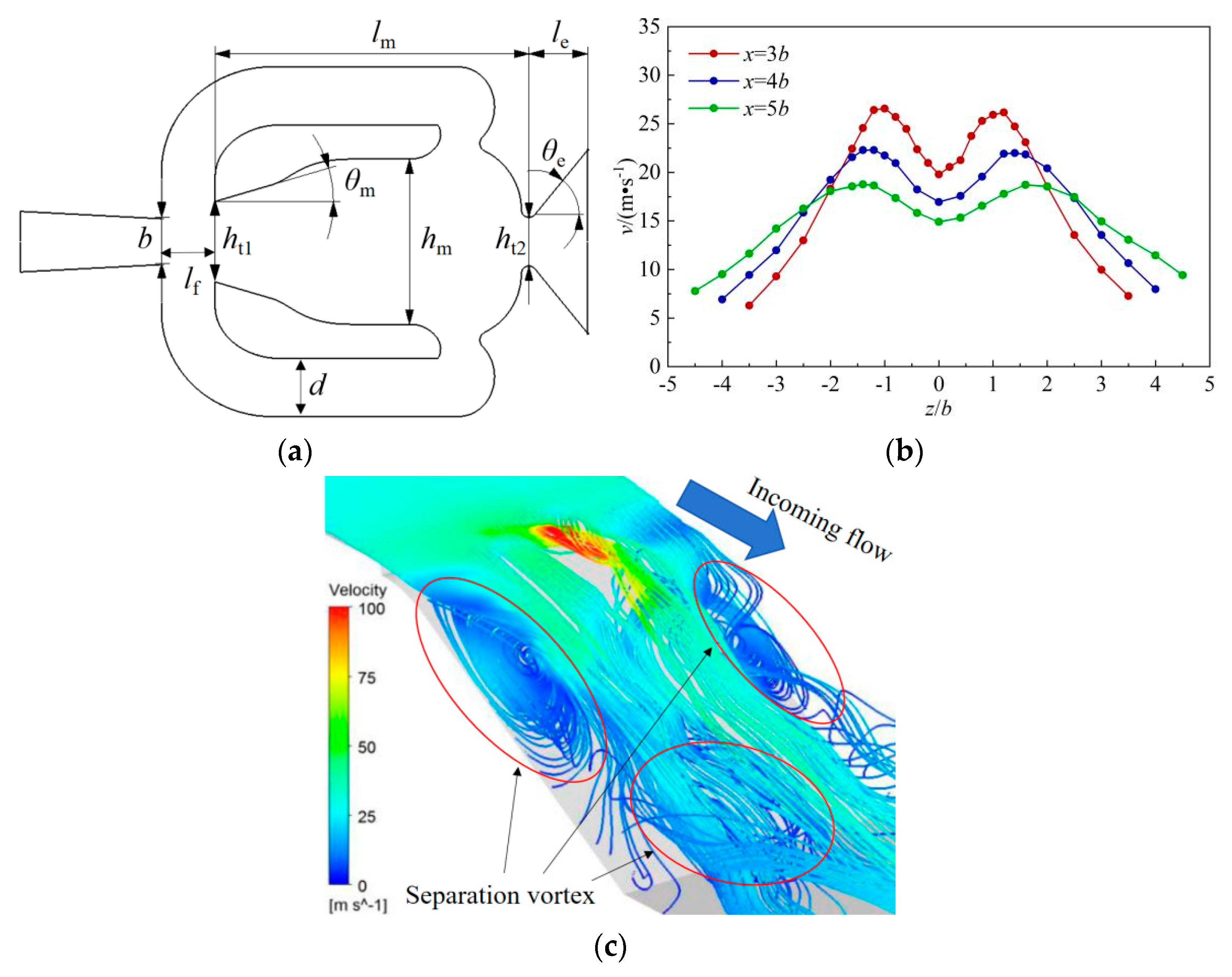
2.1. Oscillating Jet Actuator

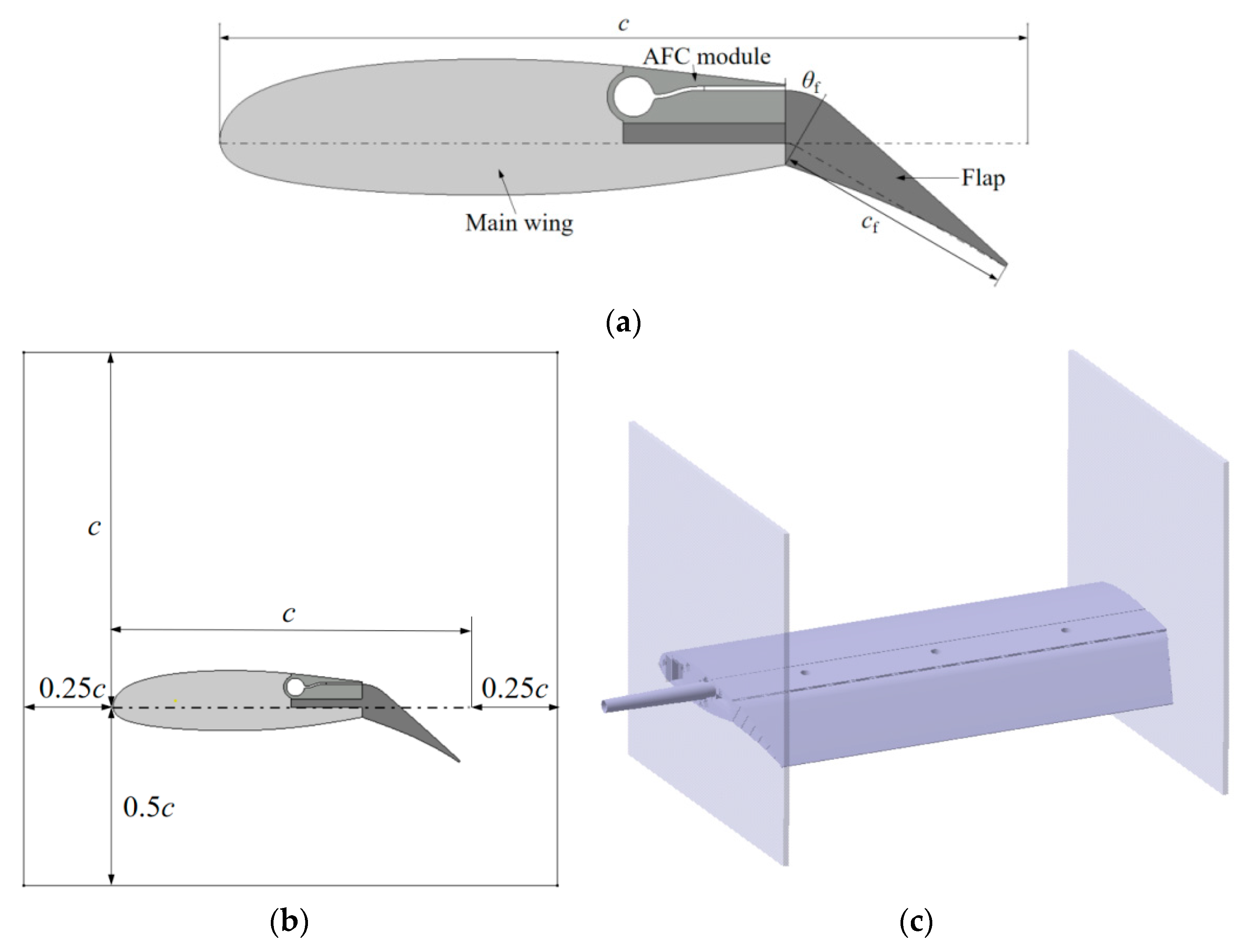
The object of this study is a single feedback channel actuator, which consists of an inlet, a feedback channel, a mixing section and an expansion section. The geometric parameters are shown in Figure 1, namely, the inlet height b, the feedback channel width d = 0.6b, the feedback section length l_f = 2.4b, the first throat height h_t1 = 1.8b, the mixing section expansion angle θ_m = 25°, the mixing section height h_m, the mixing section length l_m, the second throat height h_t2 = 1.0b, the expansion angle of the expansion section θ_e and the length of the expansion section l_e. The design variables are the parameters of the mixing section (h_m, l_m) and the expansion section (θ_e, l_e). In the external flow field measurement of the actuator, take b = 10 mm and the actuator inlet size is 10 mm × 6 mm.

Figure 2 gives the oscillation process of the jet inside the actuator [34]. The fluid flows into the mixing section and the Coanda effect causes it to adhere to one side of the wall (Figure 2a), while part of the fluid flows into the separation vortex via the feedback channel (Figure 2b,c), and the separation vortex squeezes the jet to the other side (Figure 2d), which causes the jet to oscillate.

2.2. Wing Model

The separation control effect of the oscillating jet on a wing model was studied. A transport aircraft airfoil was used, as shown in Figure 3a. The wing model consists of the main wing, flap and AFC module. The wing chord length is c = 0.2 m, the wingspan is 0.4 m and the flap chord length is c_f = 0.3c. The actuators are arranged in the trailing edge of the AFC module, the blowing direction is parallel to the chord line and the height of the blowing slit is 1 mm. The angle of attack of the wing is 0°, the deflection angle of the flap θ_f is 30°, and the inlet height b of the actuator is taken to be 2 mm (the space inside the AFC module is limited).

The wing is processed by photosensitivity rapid prototyping technology with a processing accuracy of 0.1 mm. Square plexiglass panels (1.5c) were mounted on both sides of the wing, as shown in Figure 3b. The wing model after the installation of the panels is shown in Figure 3c.

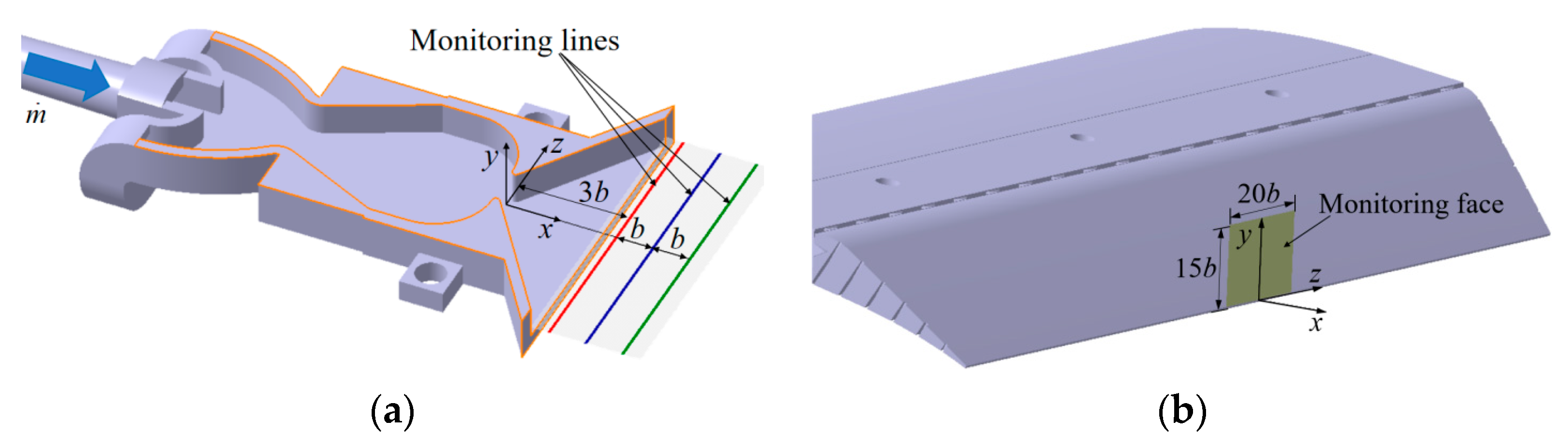
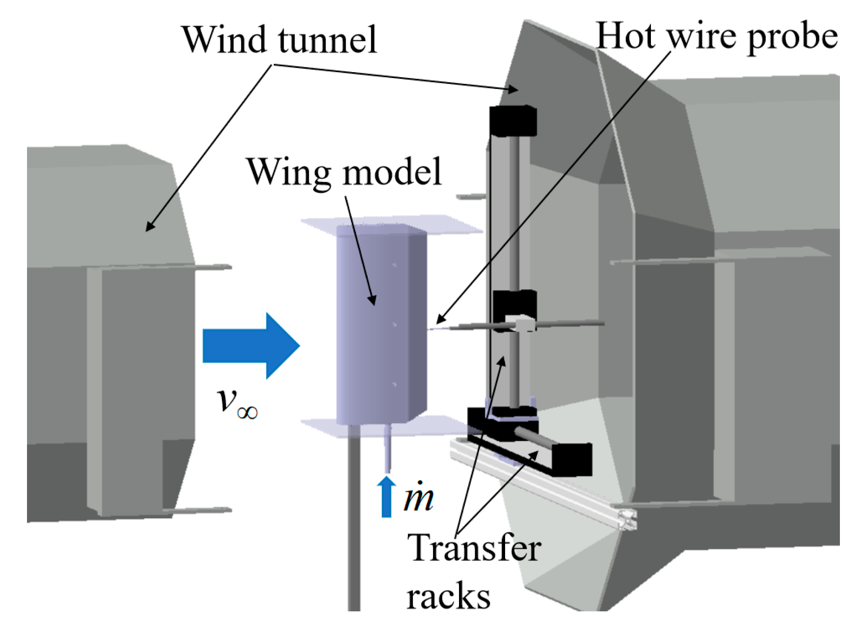
2.3. Experimental Equipment

A high-pressure gas source was used (pressure up to 0.8 MPa), and the flow rate was controlled using an OMEGA (Norwalk, CT, USA) flow meter. The flow measurement range was 0~50 g/s and the adjustment accuracy was less than 0.1 g/s. A Hanghua (Dalian, China) Constant Temperature Anemometer and a HW1A hot wire (a gold-plated tungsten wire with a length of 2 mm and a diameter of 5 μm) were used to measure the external flow field of the actuator and the wing wake. The velocity measurement error was within 3%. The sampling frequency was set to be 10 kHz, the sampling time for each sampling point was 1 s, and the distance between both sampling points was 2 mm.

The hot-wire scanning planes are shown in Figure 4, and the coordinate origin is the center of the second throat during the actuator external flow field measurement. The time-averaged velocity distribution on the monitoring lines (3b, 4b, and 5b from the second throat) was measured (Figure 4a); for the wing wake measurement, the coordinate origin at the trailing edge of the wing center profile and the time-averaged velocity distribution in the yz plane were measured (Figure 4b).

The wing wake measurement was carried out in the basic aerodynamics research wind tunnel of China Aerodynamic Research and Development Center. The size of the test section was 0.7 m × 0.7 m × 0.85 m, the maximum wind speed was about 50 m/s and the wind speed used in the experiment was 20 m/s. The arrangement of the wing model and the hot-wire probe in the test section is shown in Figure 5.

The jet velocity was calculated using the theory of compressible flow according to Equations (1) and (2) to establish the relationship between the flow rate $\dot{m}$ and the jet velocity v_j where γ is the specific heat ratio, R is the gas constant, n_p is the ratio of the total pressure of the jet to the static pressure in the far field, P_∞ and T_∞ are the static pressure and static temperature in the wind tunnel, T₀ is the total temperature of the jet and S_j is the inlet area of the actuator (for the AFC module, it is the sum of the inlet area of all actuators). In the actuator external flow field measurement, given that $\dot{m}$ is 7 g/s, the corresponding v_j is 100 m/s. In the wing wake measurement, Equation (3) was used to calculate the momentum coefficient C_μ where q_∞ is the velocity pressure of the incoming flow and S_ref is the reference area of the wing model.

$$v_{\mathrm{j}}=\sqrt{{\displaystyle \frac{2\gamma R{T}_{\infty }}{\gamma -1}}(n_{\mathrm{p}}^{(\gamma -1)/\gamma }-1)}$$

(1)

$$\dot{m}=S_{\mathrm{j}}{v}_{\mathrm{j}}{\rho }_{\mathrm{j}}=S_{\mathrm{j}}{v}_{\mathrm{j}}{\displaystyle \frac{p_{\infty }{n}_{\mathrm{p}}^{(\gamma -1)/\gamma }}{R{T}_0}}$$

(2)

$$C_{\mathsf{\mu }}={\displaystyle \frac{\dot{m}{v}_{\mathrm{j}}}{q_{\infty }{S}_{\mathrm{ref}}}}$$

(3)

3. Optimization Methods

3.1. Optimization Objectives

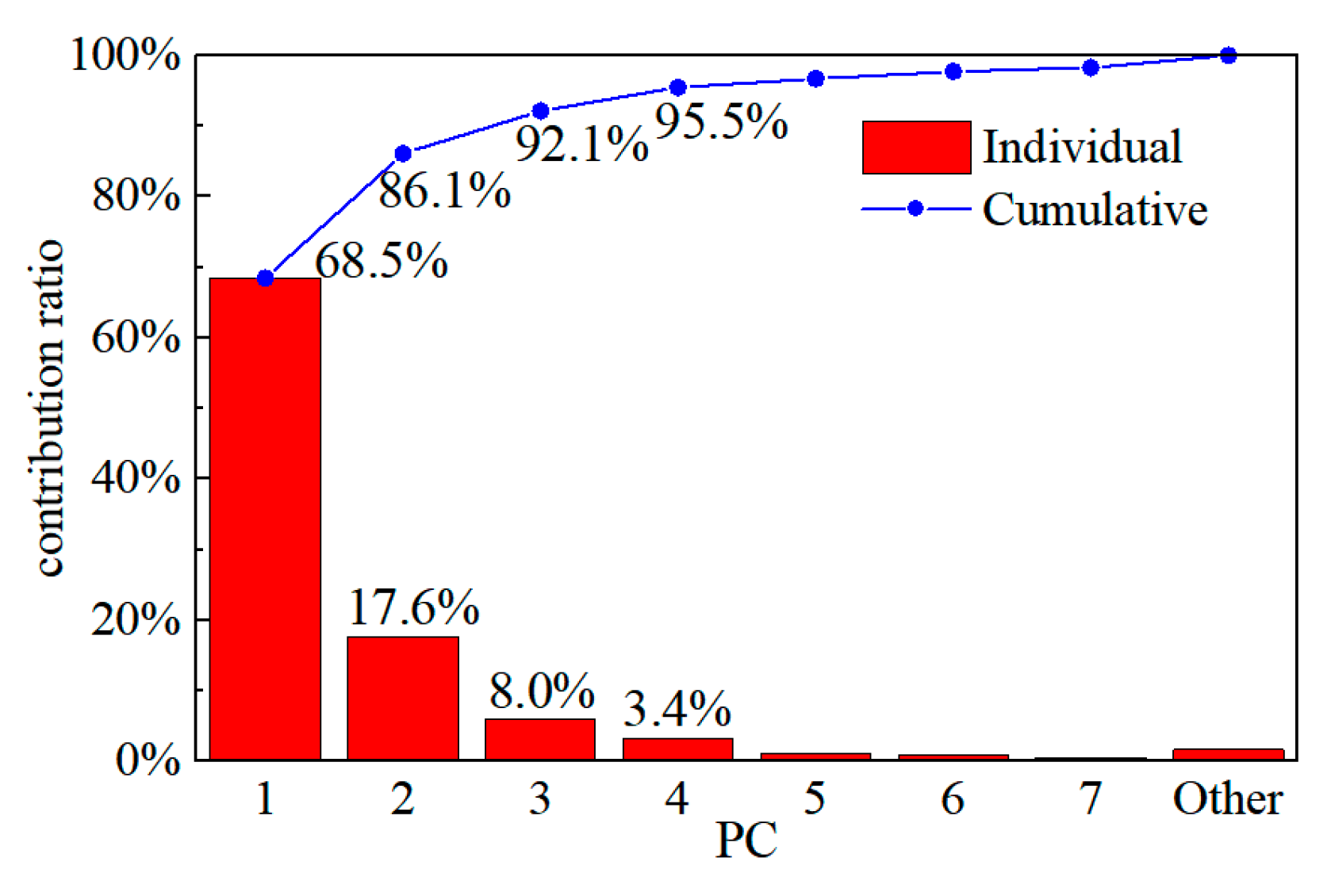
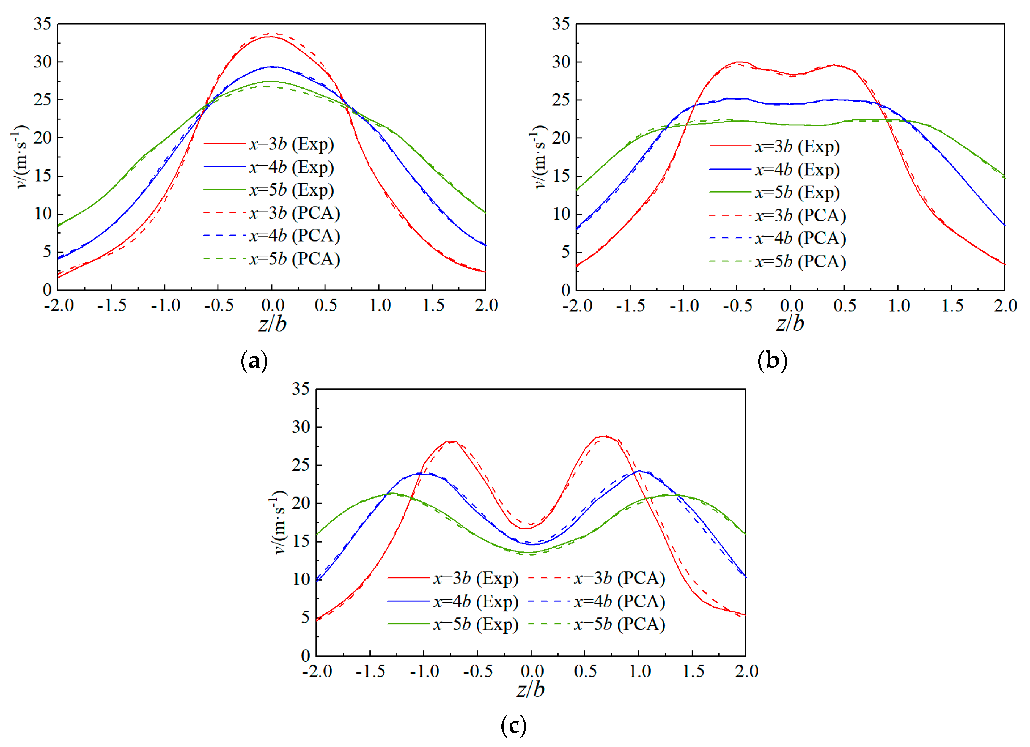
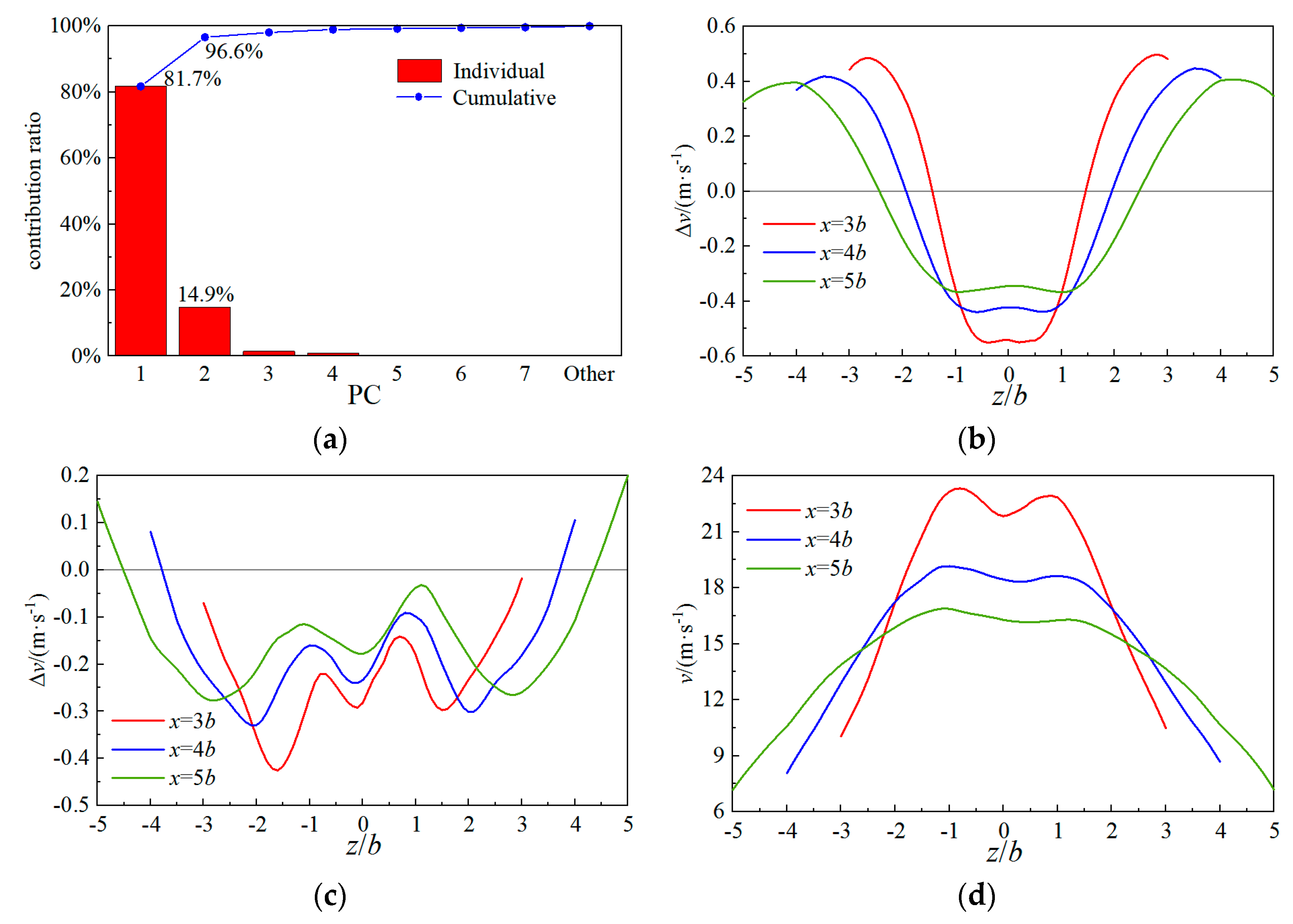
Sun [34] compared the effect of peak velocity, oscillation frequency, sweeping uniformity and range of the jet on the separation flow control, and the results show that the sweeping uniformity and range of the jet have the greatest influence on the control effect. Taking a typical actuator is commonly used in the literature as an example (Figure 6a), the external time-averaged velocity distributions of the actuator are measured as shown in Figure 6b. It can be seen that the velocity at z = ±1.5b is higher than the velocity in the center.

Sun [34] pointed out that this is due to the stagnation of the jet on both sides, resulting in more momentum being transferred to both sides than to the center, leading to the separation zone in the middle of the deflection flap (Figure 6c). The limited sweeping range of the jet (the span of the deflection flap is 16b) causes the separation zone to also appear on both sides of the deflection flap (Figure 6c), resulting in a poor control effect, so the more uniform the jet sweeping and the larger the jet sweeping range, the better the control effect.

Since the degree of jet sweeping uniformity and range are both related to the time-averaged velocity distribution outside the actuator, the actuator evaluation parameters based on the velocity distribution are proposed. The velocity distribution between the two peaks on each monitoring line was extracted, and the degree of uniformity of the momentum transfer from the jet to the flow field c_e is as shown in Equation (4), where v_i is the velocity at each sampling point, v_max is the maximum peak velocity and the closer c_e is to 1, the more uniform the jet sweeping. The distance between the two peaks z_j indicates the jet sweeping range, and the average values of c_e and z_j on three monitoring lines were subsequently used to evaluate the performance of the actuator. Using the above method, c_e = 0.608 and z_j = ±1.3b for the typical actuator were calculated from Figure 6b.

$$c_{\mathrm{e}}={\displaystyle \frac{{\displaystyle \sum _{\mathrm{i}=1}^{\mathrm{n}}{\left(\frac{v_{\mathrm{i}}}{v_{\max }}\right)}^2}}{\mathrm{n}}}$$

(4)

3.2. PCA Methods

The evaluation parameters in Section 3.1 are only applicable in the case where there are two peaks in the velocity distribution (bimodal distribution), and are not applicable to more complex velocity distribution patterns. While any velocity distribution can be expressed as a linear combination of a series of modals, as long as it is clear that each order of the modal impacts on the c_e and z_j, the c_e and z_j of the velocity distribution can be obtained. Therefore, modal decomposition of the velocity distributions was performed to establish actuator evaluation parameters based on the modal characteristics, and the physical meaning of each modal was analyzed in conjunction with the evaluation parameters in Section 3.1.

The modal decomposition was performed using principal component analysis (PCA) method. The sample set X consists of n samples (X = {x₁, x₂, ⋯, x_n}), each sample with dimension p (x_i = (x_i1, x_i2, ⋯, x_ip)). In the sample set consisting of actuator external velocity distributions, n is the number of actuators, p is the number of sampling points and x_i is the external velocity distribution of the i-th actuator. Each sample is centered with samples mean μ, and centered sample $\overline{x_{\mathrm{i}}}=x_{\mathrm{i}}-\mu$, $\overline{X}$ denotes the set of centered samples.

The covariance matrix COV of $\overline{X}$ was calculated as shown in Equation (5), the eigen-decomposition of the covariance matrix was performed to obtain the eigenvalue λ_i and the eigenvector V_i (modal). Principal component (modal coefficient) $\mathrm{PCi}=\overline{x_{\mathrm{i}}}\cdot V_{\mathrm{i}}$, which represents the projection of the sample set onto each eigenvector. The ratio of λ_i to the sum of all the eigenvalues is the contribution ratio of i-th modal, the larger the contribution ratio, the more original data features the modal contains.

Using the Equation (6) to reconstruct $\overline{X}$, which is the product of principal components and modals. Usually, the first k orders (k << n) of modals contain a large number of features (>90%) of the original data [35]; therefore, it is sufficient to compute only the sum of the first k terms in Equation (6) to reduce the n-dimensional data to k dimensions.

$$COV={\displaystyle \frac{1}{n}}\overline{X} {\overline{X}}^T$$

(5)

$$\overline{X}={\displaystyle \sum _{\mathrm{i}=1}^n\mathrm{PCi}\cdot V_{\mathrm{i}}}$$

(6)

3.3. Kriging Surrogate Model

After using the PCA method to reduce the dimension of velocity distribution, it is only necessary to establish surrogate models of principal components on geometric parameters to obtain the relationship between geometric parameters and velocity distribution. The kriging model was used for interpolation. This model consists of two parts, the regression model and the stochastic model, as shown in Equation (7), where f(x) is the global trend model, usually taken as the constant β₀, which is the average of all sample data, z(x) is a static stochastic process with mean μ = 0, variance σ² and covariance Cov(z(x⁽ⁱ⁾), z(x^(j))) = σ² R(θ, x⁽ⁱ⁾, x^(j)), where R(θ, x⁽ⁱ⁾, x^(j)) is the correlation function. The Gaussian exponential model as shown in Equation (8) is often used, where the subscript k is the k-th component of each vector.

$$\widehat{y}(x)=f(x)+z(x)$$

(7)

$$R_{\mathrm{k}}({\theta }_{\mathrm{k}},x_{\mathrm{k}}^{(i)},x_{\mathrm{k}}^{(j)})=\exp (-{\theta }_{\mathrm{k}}{\left|x_{\mathrm{k}}^{(i)}-x_{\mathrm{k}}^{(j)}\right|}^2)$$

(8)

The unknown variables in the model are θ, and the maximum likelihood estimation method is usually used to obtain all unknowns. The maximum likelihood function is shown in Equation (9), and a global search can be performed to obtain the θ that maximizes ln(L). The estimated value of the unknown point is shown in Equation (10), where R⁻¹(y − β₀) can be obtained from all sample data, and r^T(x) is composed of the correlation function values between the unknown point and the sample points, as shown in Equation (11).

$$\ln (L)\approx -{\displaystyle \frac{\mathrm{n}}{2}}\ln ({\displaystyle \frac{{(y-{\beta }_0)}^{\mathrm{T}}{R}^{-1}(y-{\beta }_0)}{\mathrm{n}}})-{\displaystyle \frac{1}{2}}\ln \left|R\right|$$

(9)

$$\widehat{y}(x)={\beta }_0+r^{\mathrm{T}}(x)R^{-1}(y-{\beta }_0)$$

(10)

$$r^T(x)=[R(x^{(1)},x)\hspace{0.33em}R(x^{(2)},x)\cdots R(x^{(\mathrm{n})},x)]$$

(11)

The prediction error Δy is used to evaluate the prediction accuracy of the surrogate model, as shown in Equation (12), where $\widehat{y}$ is the predicted value and y is the actual value; the smaller the Δy, the higher the prediction accuracy of the surrogate model. It is usually considered that the prediction accuracy meets the demand when Δy < 10%.

$$\Delta y=\left|{\displaystyle \frac{\widehat{y}-y}{y}}\right|$$

(12)

3.4. Multi-Objective Optimization Methods

The NSGA-II multi-objective genetic algorithm was used in the present study. This algorithm is mainly used for solving optimization problems with multiple conflicting objectives and is able to directly compute the optimal solution set (Pareto solution set). The Pareto solution set represents all the possible optimal solutions, and for any solution in the solution set, there does not exist another solution that outperforms it on all objectives. Setting the population size to 50, crossover probability to 0.8, variance probability to 0.05, and the maximum number of iterations to 1000, the steps of the algorithm are:

• Population initialization: Randomly generate the initial population, where each individual represents a solution.
• Evaluation: Calculate the value of the objective function for each individual.
• Non-dominated sorting: Compare all individuals in the population pairwise to determine the set of individuals p_s dominated by each individual s (each objective is inferior to the individual s) and the number of individuals n_s dominated by s (there is at least one objective exceeding the individual s) and classify the individuals with n_s = 0 as the first rank (non-dominated individuals), which are the optimal solutions. Then sort the individuals recursively until they are all assigned to a certain rank.
• Crowding degree calculation: Sort the individuals within each rank separately according to each objective function value, calculate the distances between neighboring individuals, accumulate these distances to obtain the crowding degree of the individual and arrange all individuals within the rank in descending order according to the crowding degree.
• Selection and updating: Perform the binary tournament selection strategy and select the individual with low non-dominance rank and high crowding degree as the parent.
• Genetic operation: Perform the crossover operation on the selected parent individuals to generate new offspring individuals and mutation operation on the offspring individuals to increase the population diversity.
• Merging the population: Combine the newly generated offspring with the best individuals of the previous generation to form a new generation of the population.
• Determining the termination conditions: Determine whether the termination conditions are met, such as reaching the maximum number of iterations, meeting the preset criteria for the quality of the solution or the algorithm converging. If the termination conditions are met, then output the optimal solution set and end the algorithm, otherwise, return to step 2 to continue the iteration.

A summary of the multi-objective optimization process based on the kriging model is shown in Figure 7.

4. Actuator Optimization Design

A principal component analysis was performed on the external time-averaged velocity distribution of the actuator. The modals of the velocity distribution were obtained and the influence of each order of modals on the sweeping uniformity and range of the jet was analyzed. The evaluation parameters of the actuator based on the modals are proposed and the kriging surrogate models of the modal coefficients (principal components) on the geometric parameters are established. The NSGA-II algorithm was utilized for the multi-objective optimization to obtain the optimal actuator.

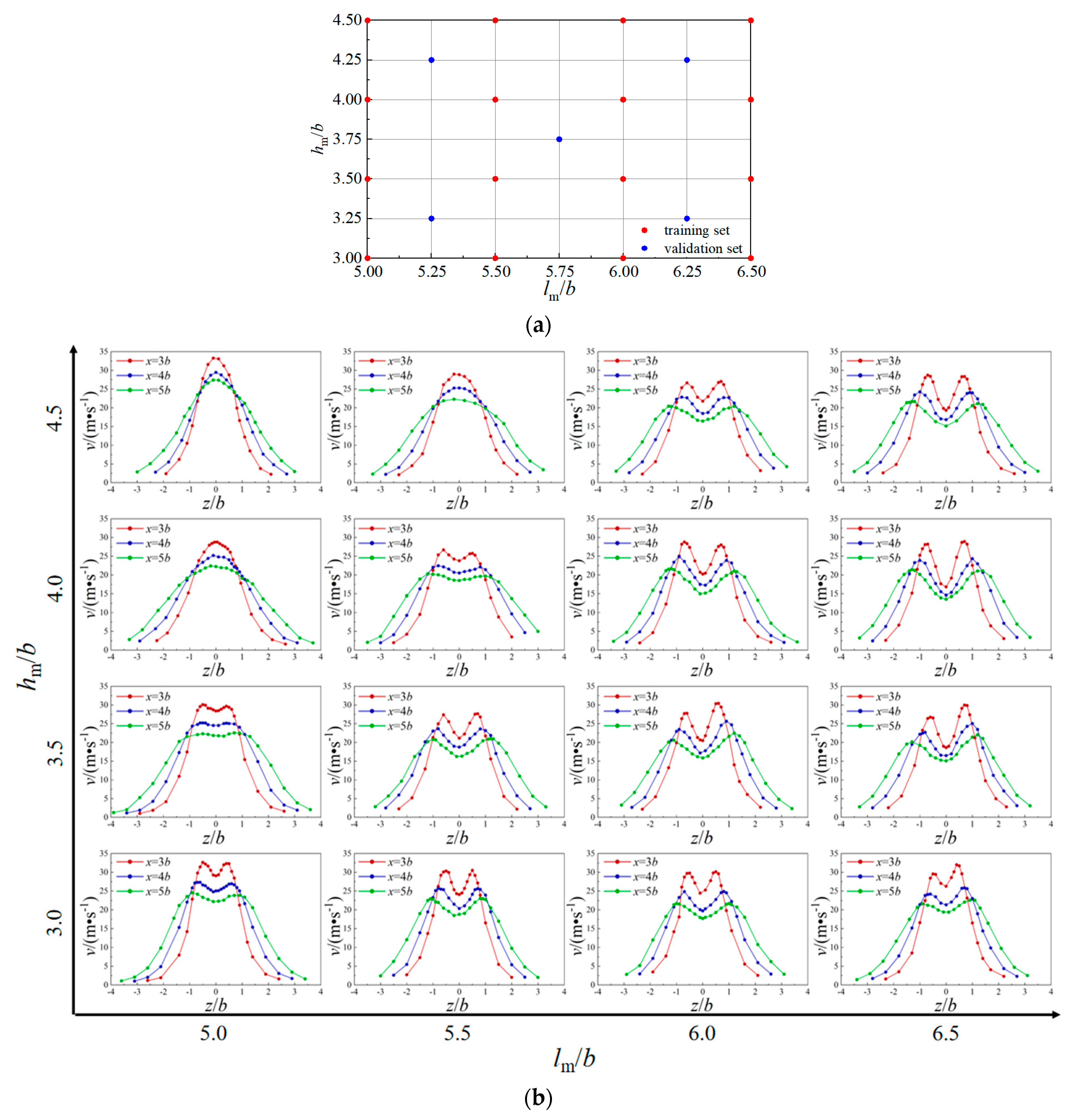
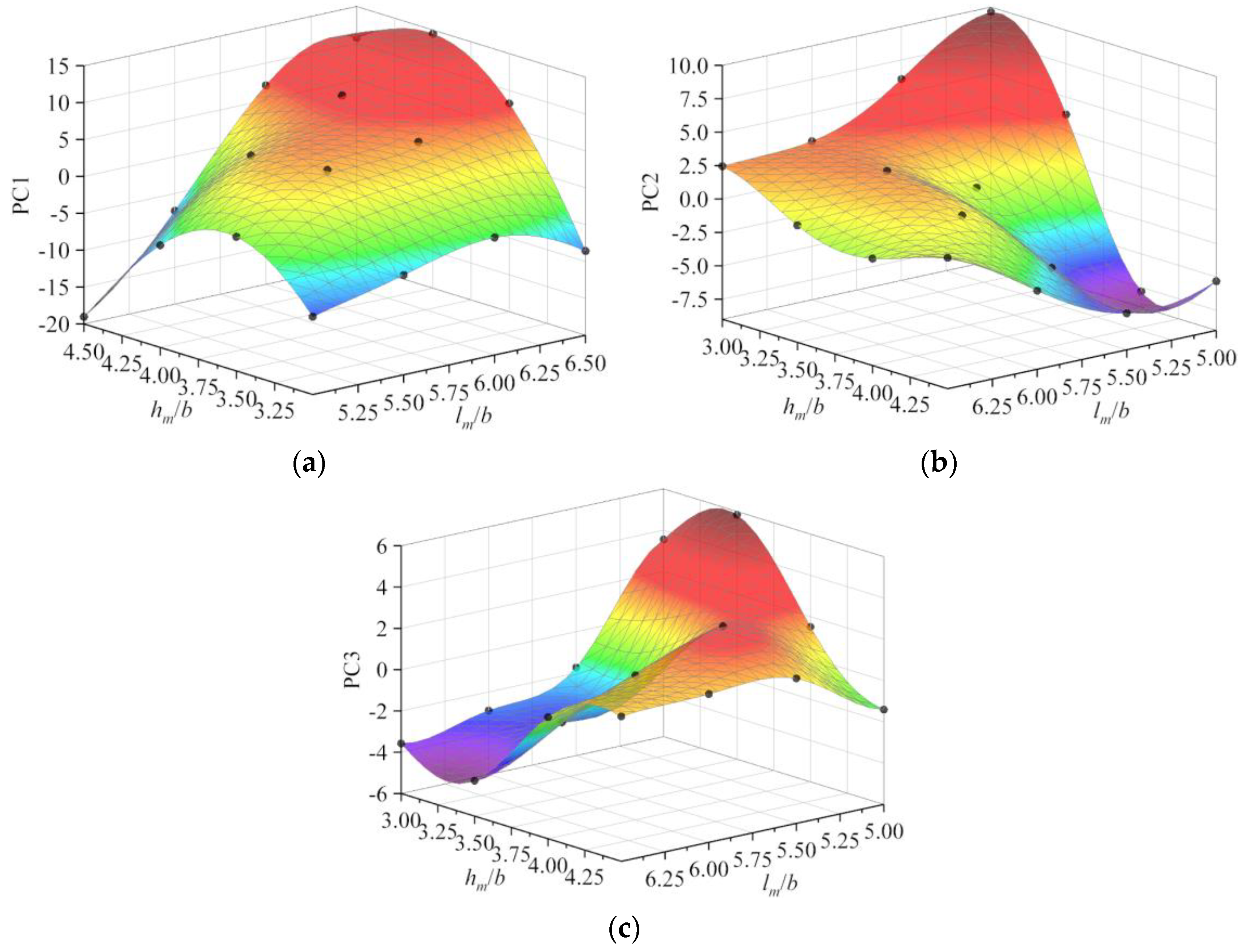
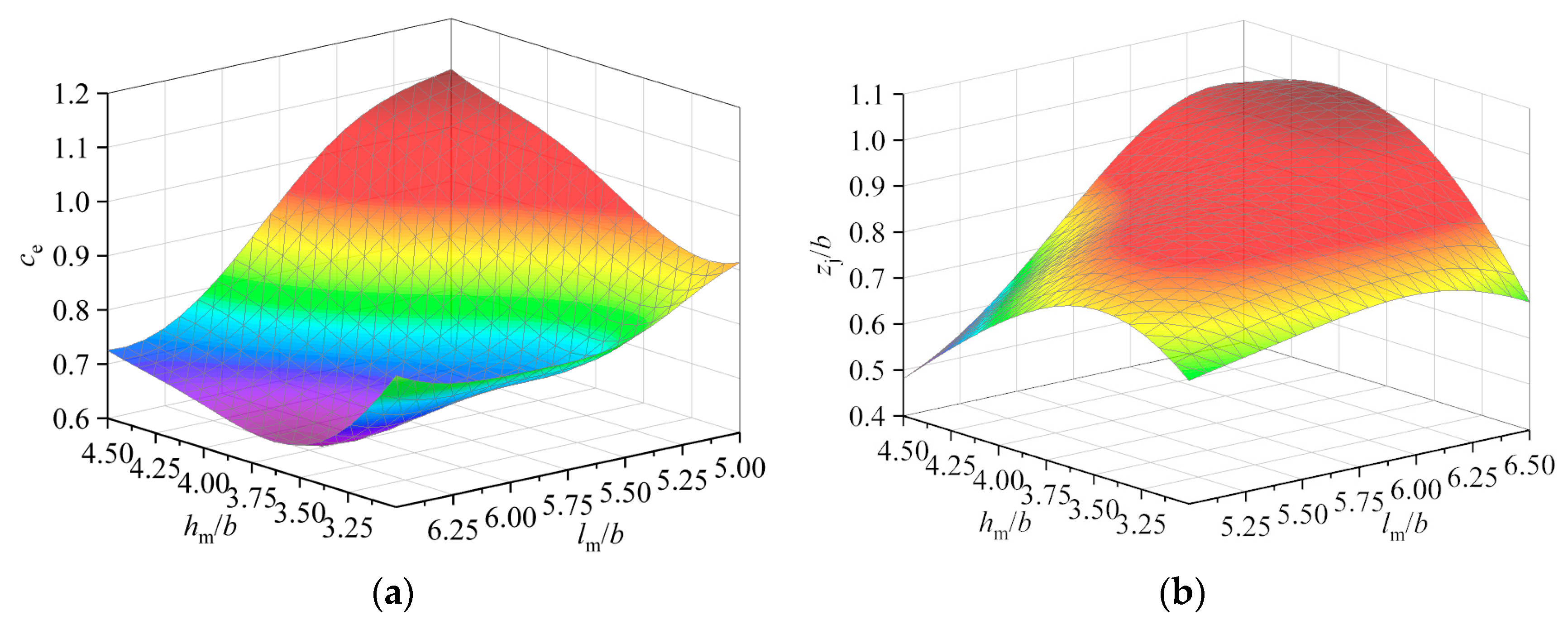
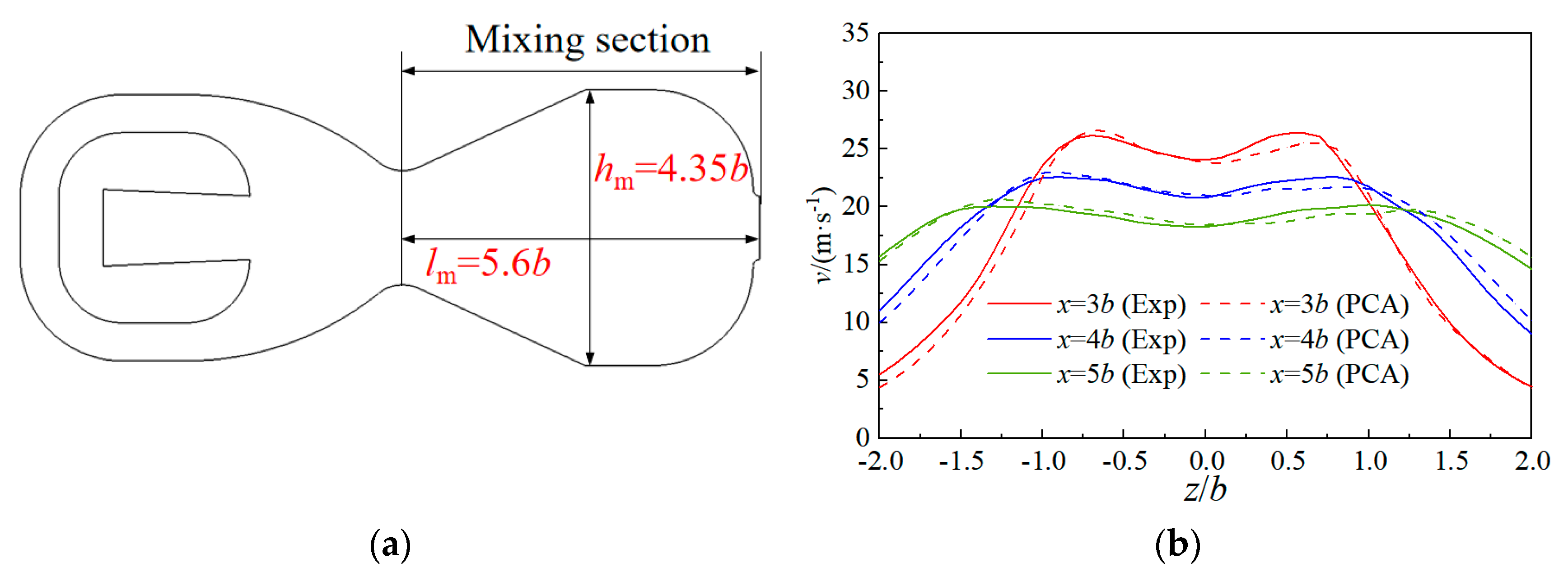
4.1. Optimization Design of Mixing Section

References [36,37] indicate that the expansion section has almost no effect on the internal flow in the mixing section, but it affects the external velocity distribution of the actuator. The expansion section is removed during the optimization of the mixing section in order to clarify the influence of the mixing section on the external flow field characteristics and eliminate the interference of the expansion section on the test results of the mixing section.

The effect of the mixing section height h_m and mixing section length l_m were analyzed. The training and validation set distributions are shown in Figure 8a. The test results of the training set were used to build surrogate models, and the test results of the validation set were used to verify the accuracy of the surrogate models.

The test results of the training set are shown in Figure 8b. There are three patterns of velocity distribution: unimodal, broad and bimodal. When l_m is small and h_m is large (l_m = 5.0b, h_m = 4.5b), the velocity distribution is unimodal; when l_m and h_m are large (l_m = 6.5b, h_m = 4.0b), the velocity distribution is bimodal; and from the unimodal to the bimodal, the broad pattern (l_m = 5.5b, h_m = 4.0b) will appear.

The unimodal velocity distribution indicates that the sweeping range of the jet is small (two peaks with small distance merge into one peak), while the minimum distance between actuators depends on the z-direction width of the actuator. If the sweeping range of the jet is smaller than the z-direction width of the actuator, there is a region between the two actuators that cannot be controlled by the jet. The bimodal velocity distribution means that the jet is not sweeping uniformly (Figure 6a); the broad pattern can increase the sweeping range while ensuring the sweeping uniformity of the jet.

With the increase in l_m, the velocity distribution pattern gradually transforms to a bimodal pattern, and the height and distance of the peaks gradually increase, which means that the increase in l_m decreases the sweeping uniformity and increases the sweeping range of the jet. With the increase in h_m, the velocity distribution pattern gradually transforms to the unimodal pattern when l_m ≤ 5.5b, and to the bimodal pattern when l_m ≥ 6.0b.

According to the analysis results of the flow field inside the actuator from Sun [34], this is due to the limited offset height of the jet in the mixing section when l_m is small. Therefore, increasing h_m prevents the jet from attaching to the wall of the mixing section, reduces the stagnation time of the jet and improves the uniformity of the jet sweeping (Figure 9a). When l_m is large, increasing h_m can enlarge the separation vortex in the mixing section, and the jet offset height increases under the compression conditions of the separation vortex, thus increasing the jet sweeping range (Figure 9b).

In order to quantitatively describe the velocity distribution pattern, the experimental results were subjected to principal component analysis, and the contribution of each principal component was obtained as shown in Figure 10. The cumulative contribution ratio of the first three principal components is more than 90%; this means that the first three orders of modals contain more than 90% of the information of the flow field, so the flow field was subsequently reconstructed by using the first three orders of modals.

The results of principal component analysis are shown in Figure 11. The first two modals have a bimodal distribution; the first modal has a low valley in the middle and a large distance between the peaks on both sides, the second modal has two high peaks and small distance between the peaks and the third modal has a unimodal distribution with the highest peaks. The mean flow field is the average of all the velocity distribution measurement results, and it is a bimodal distribution with a slight concavity in the middle. The velocity distribution of each configuration can be obtained by superimposing the perturbation on the mean flow field, and the amount of perturbation is the linear combination of the first three modals (the weight of each modal is the principal component).

In order to verify the reconstruction effect of the PCA method, the velocity distributions of all samples were reconstructed using the first three orders of modals, and the reconstruction accuracy was evaluated using the goodness-of-fit R² as shown in Equation (13), where y_i is the data of the i-th sample point, ${\widehat{y}}_i$ is the reconstructed value, and $\overline{y}$ is the average value of the data of all sample points. R² = 0.9872 was calculated, some of the reconstruction results are shown in Figure 12. The reconstruction results are in good agreement with the experimental results (the reconstruction effect of all actuators is good); the unimodal, broad and bimodal distributions can be reconstructed well by using only the first three orders of modals, which verifies the effectiveness of the PCA method.

$$R^2=1-{\displaystyle \frac{{\displaystyle \sum _{i=1}^n{(y_i-{\widehat{y}}_i)}^2}}{{\displaystyle \sum _{i=1}^n{(y_i-\overline{y})}^2}}}$$

(13)

The effect of each order of modals on the velocity distribution pattern was then analyzed. The evaluation parameters of all bimodal distributions were calculated using the method in Section 3.1, and the interaction between the evaluation parameters and each principal component was analyzed via regression. The regression equations are shown in Equations (14) and (15), R² is 0.9535 and 0.9998, indicating that the regression effect is good.

The coefficient value of the regression equation represents the influence level of each principal component on c_e and z_j; all the three principal components have a great influence on c_e and PC3 has the greatest influence, while only PC1 has a great influence on z_j. It can be seen from Figure 11, that the first two orders of modals are bimodal distributions, while the third order modal is a unimodal distribution. If PC1 and PC2 are negative, and PC3 is positive, then the first two orders of modals increase the velocity in the middle of the mean flow field and reduce the velocity on both sides, while the third-order modes will directly increase the velocity in the middle of the mean flow field, so that the c_e increases. The third modal has the greatest impact on c_e due to its maximum peak velocity.

Increasing the principal component of a modal can increase z_j only when the peaks distance of that modal is greater than the peaks distance of the averaged flow field. It can be seen from Figure 11 that the velocity peak distance of the mean flow field is 0.77b, while the velocity peak distances of the first two orders of modals are 1.43b and 0.87b. The third modal is a unimodal distribution, so it is obvious that the first modal has the greatest influence on z_j.

It is worth noting that c_e and z_j have opposite trends with each principal component (except for the constant term, the sign of each regression coefficient in the two equations is opposite). This means that increasing c_e inevitably leads to a decrease in z_j; therefore, both evaluation parameters must be coordinated in the optimization design phase.

$$c_{\mathrm{e}}=0.8432-0.012\mathrm{PC}1-0.012\mathrm{PC}2+0.0205\mathrm{PC}3$$

(14)

$$z_{\mathrm{j}}=0.7933+0.016\mathrm{PC}1+0.0035\mathrm{PC}2-0.003\mathrm{PC}3$$

(15)

It can be seen from Figure 8 that there are unimodal distributions in the mixing section measurement results. The evaluation parameters proposed in Section 3.1 cannot be used, but rounding off these samples reduces the number of samples and the accuracy of the surrogate models. Therefore, using Equations (14) and (15), c_e and z_j were calculated to establish kriging surrogate models for the first three principal components on h_m and l_m, as shown in Figure 13. The results of the validation set samples and the predictions of the surrogate models are shown in

Table 1. Test set samples and surrogate model prediction accuracy.

hm/b	lm/b	ΔPC1	ΔPC2	ΔPC3
3.25	5.25	6.67%	3.61%	3.17%
4.25	5.25	9.44%	4.99%	7.20%
3.75	5.75	1.36%	1.02%	8.87%
3.25	6.25	8.61%	4.59%	3.18%
4.25	6.25	1.38%	1.21%	1.97%

. It can be seen that Δy < 10%, which means that the prediction accuracy of the surrogate models meets the requirement.

The calculated c_e and z_j are shown in Figure 14. The optimization objective was to maximize c_e and z_j, but the velocity distribution is unimodal (to be rounded off) when c_e > 1, so the exterior penalty function method was used: if c_e > 1, then c_e = 0.

The NSGA-II algorithm was utilized to perform the multi-objective optimization. The generated Pareto front and optimization variables are shown in Figure 15. The larger the c_e, the smaller the z_j, consistent with the trend shown in Equations (14) and (15).

Although reducing c_e in exchange for a larger z_j may be beneficial to the control effect, the expansion section parameters have a greater effect on z_j than the mixing section parameters (Section 4.2), so the solution with a large c_e is selected in this chapter (c_e ≥ 0.95), and the final choices are h_m = 4.35b and l_m = 5.6b (c_e = 0.96 and z_j = 0.81b), as shown in Figure 16a. The selected solution was experimentally validated and compared with the surrogate model prediction results as shown in Figure 16b. The two are in good agreement, indicating that the surrogate model prediction results are accurate.

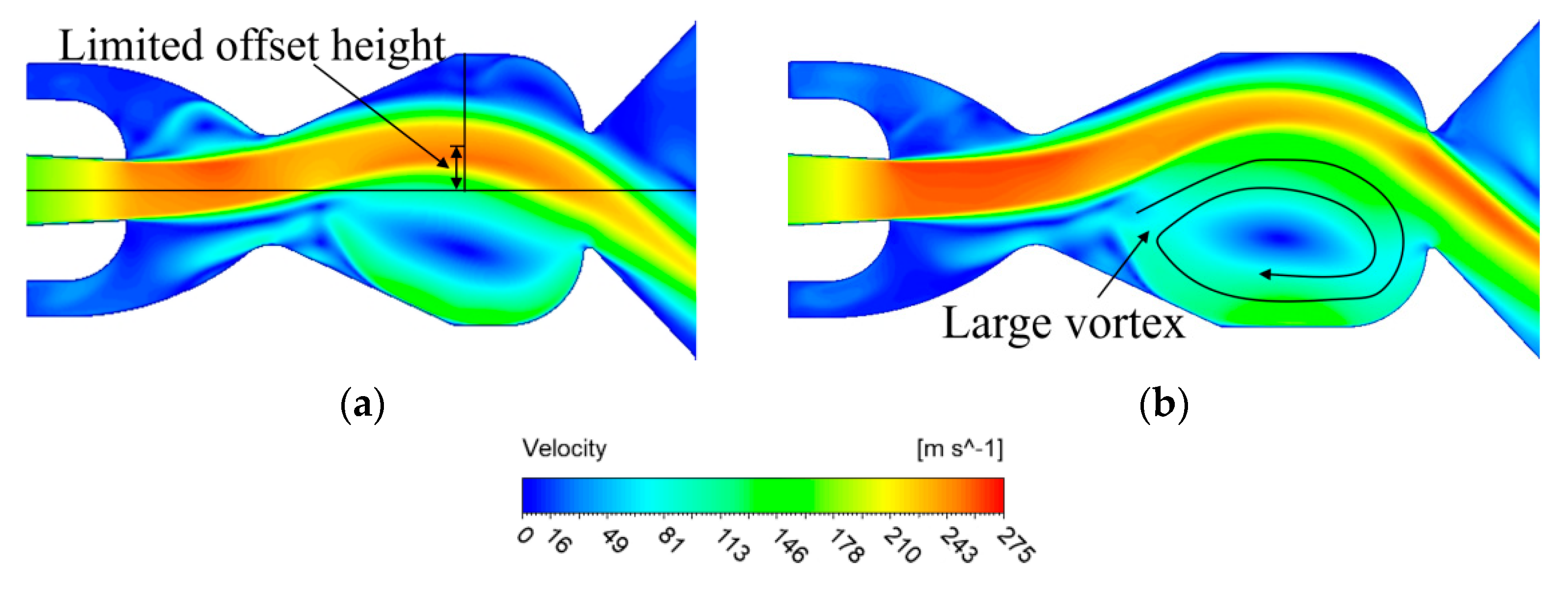
4.2. Optimization Design of Expansion Section

This section analyzes the effects of the expansion angle θ_e and the length l_e of the expansion section. The training and validation set distributions are shown in Figure 17a, and the test results of the training set are shown in Figure 17b. With an increase in θ_e, the time-averaged velocity distribution gradually transforms from a bimodal distribution to a broad distribution, which means that increasing θ_e can improve the degree of sweeping uniformity of the jet. With an increase in l_e, the velocity distribution is gradually transformed to a bimodal distribution when θ_e ≤ 45°, but the influence of l_e on the velocity distribution is obviously reduced when θ_e ≥ 50°.

The analysis of the flow structure in the expansion section based on Sun [34] (Figure 18). When θ_e is small, the interaction between the jet and the wall of the expansion section is strong and a separation vortex is formed between them to hinder the deflection of the jet, so that the jet is stagnant on both sides. At this time, an increase in l_e increases the separation vortex and strengthens the interaction between them, so the velocity distribution is converted to a bimodal distribution; when θ_e is large, the jet is farther away from the wall, and the interaction between them is weak, so the influence of l_e is reduced.

The velocity distribution patterns were then quantitatively analyzed, and the experimental results were subjected to principal component analysis, as shown in Figure 19. The cumulative contribution ratio of the first two principal components is more than 90%; the first modal has the characteristics of a bimodal and broad distribution at the same time, with two peaks, and there is a plateau area at the valley (if PC1 is negative, the PC1∙model1 has an approximately broad distribution). The distance of the two peaks and the peak-valley value (difference between the peaks and the valley) are large; the second modal is a multimodal distribution (three negative peaks), the peak-valley value is small, and the distance between peaks on both sides is smaller than that of model1. The mean flow field is approximated as a broad distribution.

The influence of various modals on the velocity distribution pattern was analyzed using the method shown in Section 4.1, and the regression equations were obtained as shown in Equations (16) and (17), R² is 0.9434 and 0.9429, indicating that the regression effect is good. It can be seen that c_e is only related to PC1 (adding PC2 to the equation has little effect on the regression effect), while z_j is related to both.

$$c_{\mathrm{e}}=0.8756-0.01\mathrm{PC}1-{(0.02\mathrm{PC}1)}^2$$

(16)

$$z_{\mathrm{j}}=1.683+0.064\mathrm{PC}1+0.03\mathrm{PC}2$$

(17)

Analyzing the causes in conjunction with Figure 19, the peak-valley value of model1 is large. If PC1 is positive, then the velocity on both sides of the mean flow field will increase and the velocity in the middle will be reduced in PC1∙model1; otherwise, the velocity on both sides of the mean flow field will be reduced and the velocity in the middle will be increased; the peak-valley value of model2 is small, thus, its influence on c_e is small. The distances of the two peaks of model1, model2, and the mean flow field are 3.45b, 2.13b, and 1b. It is obvious that the first two orders of modals influence z_j, and model1 has a greater effect.

Kriging surrogate models of principal components on θ_e and l_e were established, and c_e and z_j were obtained using Equations (16) and (17), as shown in Figure 20. According to

Table 2. Accuracy table for surrogate models.

θe/°	le/b	ΔPC1	ΔPC2
42.5	1.25	8.70%	8.76%
42.5	2.25	3.03%	0.22%
47.5	1.75	1.89%	3.67%
52.5	1.25	9.44%	3.23%
52.5	2.25	1.44%	5.31%

, the prediction accuracy of the surrogate models meets the requirement. The NSGA-II algorithm was utilized for optimization, and the generated Pareto front and optimization variables values are shown in Figure 21.

The larger the c_e, the smaller the z_j, and the same trend can be seen with the optimization result of the mixing section. However, when c_e is certain, z_j in the optimization result of the expansion section is obviously larger than that of the mixing section, which indicates that it is reasonable to choose a mixing section with a large c_e and increase z_j by optimizing the expansion section.

In Figure 21b, it can be seen that θ_e in the optimal solution set is distributed between 42.5° and 44.5° (the averaged value is about 43°), and l_e/b $\in$ [1.0,2.5] (c_e gradually decreases and z_j gradually increases with the increase in l_e), combining this findings with the experimental results in Figure 17, it can be seen that the optimal solution set selects a small θ_e (when θ_e < 45° the jet is close to the wall on both sides of the expansion section, and there is a strong interaction between them) and adjusts the strength of the interaction by adjusting the l_e, so as to realize the transition between the high sweeping uniformity and the large sweeping range of the jet. Therefore, θ_e = 43° is subsequently selected, and the combination of c_e and z_j which is favorable for separation control is found by changing l_e.

In summary, the geometric parameters of the optimal actuator h_m = 5.6b, l_m = 4.35b, θ_e = 43°, and l_e = 1.0b were preliminarily selected, as shown in Figure 22a. The oscillation frequency of the jet was measured using a hot wire in order to test whether the designed actuator can operate under other working conditions, as shown in Figure 22b. The results showed that the jet could oscillate stably at $\dot{m}$ = 0~24 g/s (v_j = 0~230 m/s), indicating that the actuator can operate reliably.

5. Wing Separation Flow Control

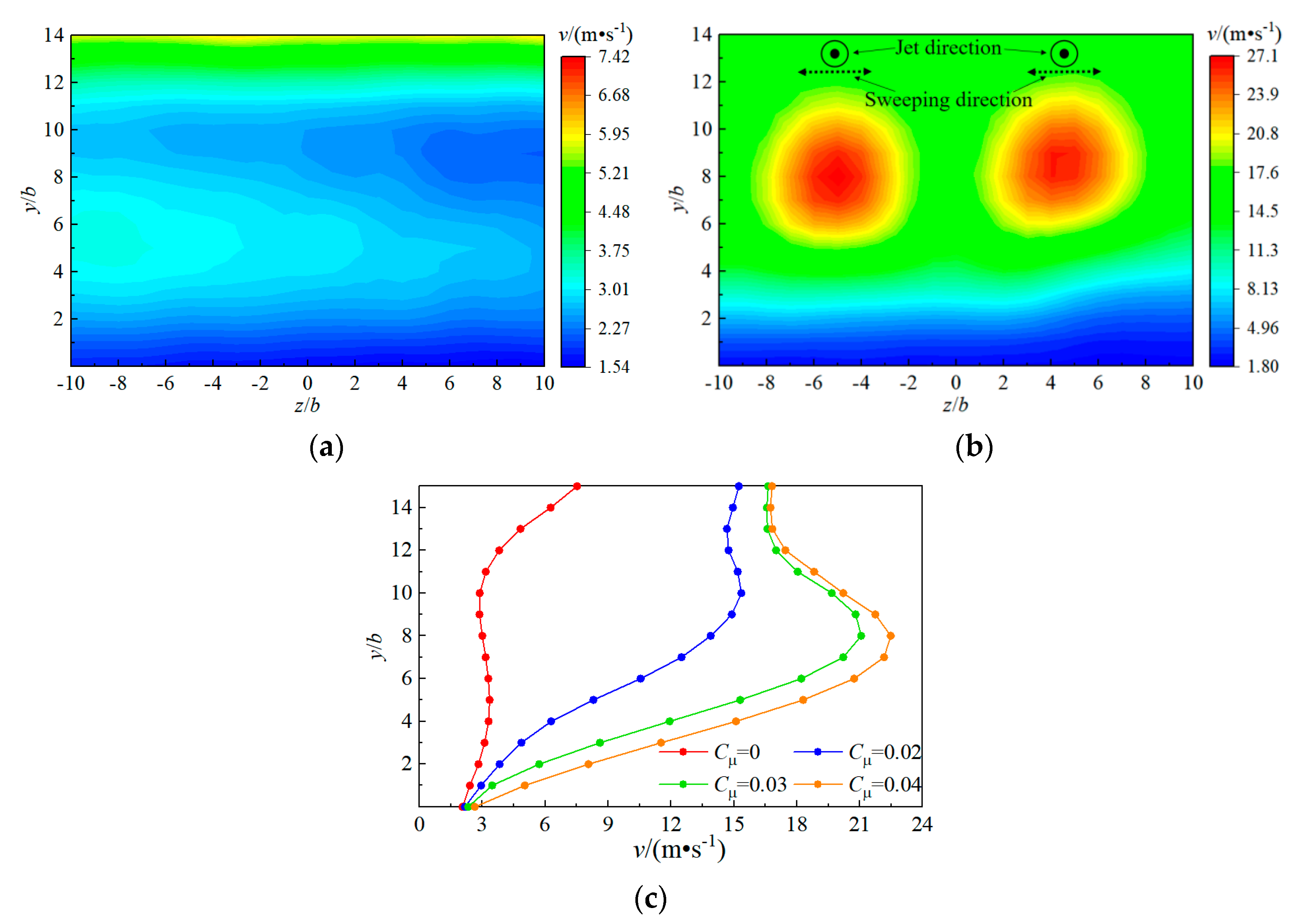
5.1. Effect of Momentum

The flow field over wing at different C_μ was analyzed. Take the actuators distance as 10b, the experimental results are shown in Figure 23. The whole monitoring surface is located in the separation zone when C_μ = 0 (Figure 23a), and the separation flow is suppressed after applying the control (Figure 23b), but due to the limited sweeping range of the jet, the velocity values between the two actuators are low. In order to facilitate the comparison of the control effect at different C_μ, the velocity was averaged along the spanwise direction, and the spanwise averaged wake was obtained as shown in Figure 23c.

In Figure 23c, the spanwise averaged velocity after applying the control increases rapidly with y and then decreases after reaching the maximum value (the jet center) and finally converges to the local outflow velocity. The lower the position of the jet center, the smaller the separation zone, the fuller the velocity distribution from the trailing edge point to the jet center and the faster the velocity convergence above the jet center. The position of the jet center is basically stable at y/b = 8 after C_μ ≥ 0.03, so it can be considered that the flow is attached on the flap. Thus, C_μ = 0.03 was selected for subsequent analysis.

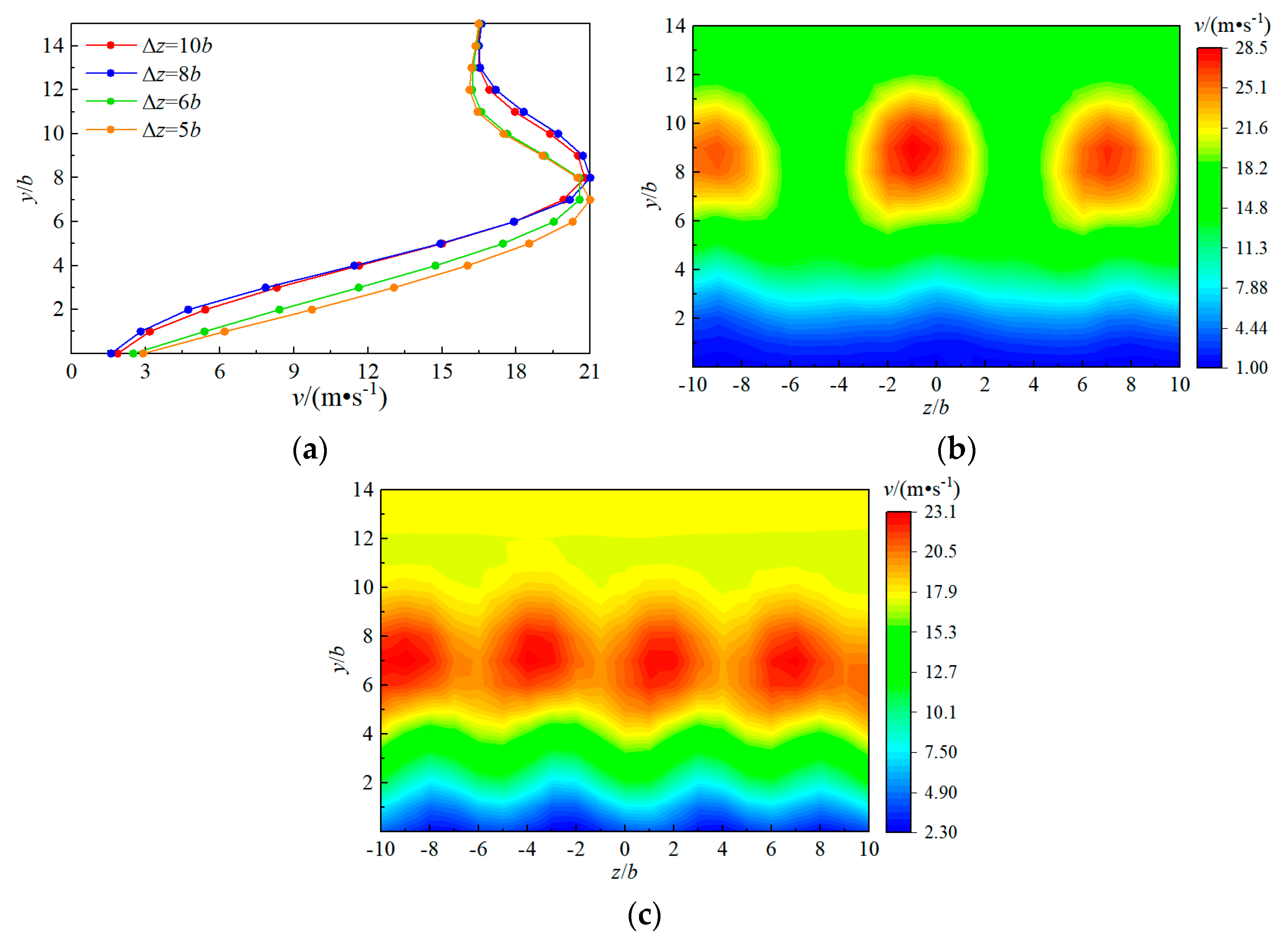
5.2. Effect of Arrangement Distance

In Figure 23b, the jet sweeping range is less than 10b. In order to improve the control effect, the actuator arrangement distance Δz should be reduced, and since the z-direction width of the actuator is less than 5b, Δz $\in$ [5b,10b] was selected. The experimental results are shown in Figure 24. The wing wake barely changes when Δz is reduced from 10b to 8b (Figure 24a), which is due to the fact that the jet sweeping range is smaller than 8b (Figure 24b). When Δz is further reduced to 6b, the jet center is obviously shifted downward, and the control effect is improved (Figure 24a). The best control effect is achieved when Δz = 5b (Figure 24c); at this time, Δz is close to the jet sweeping range, so Δz = 5b was subsequently selected.

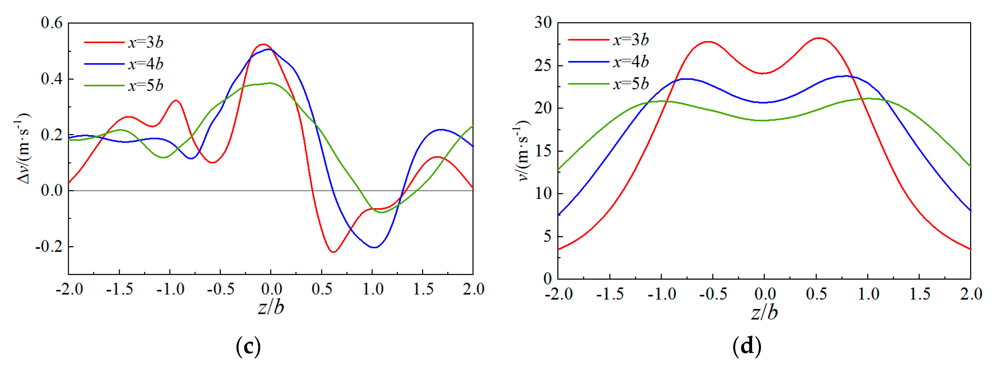
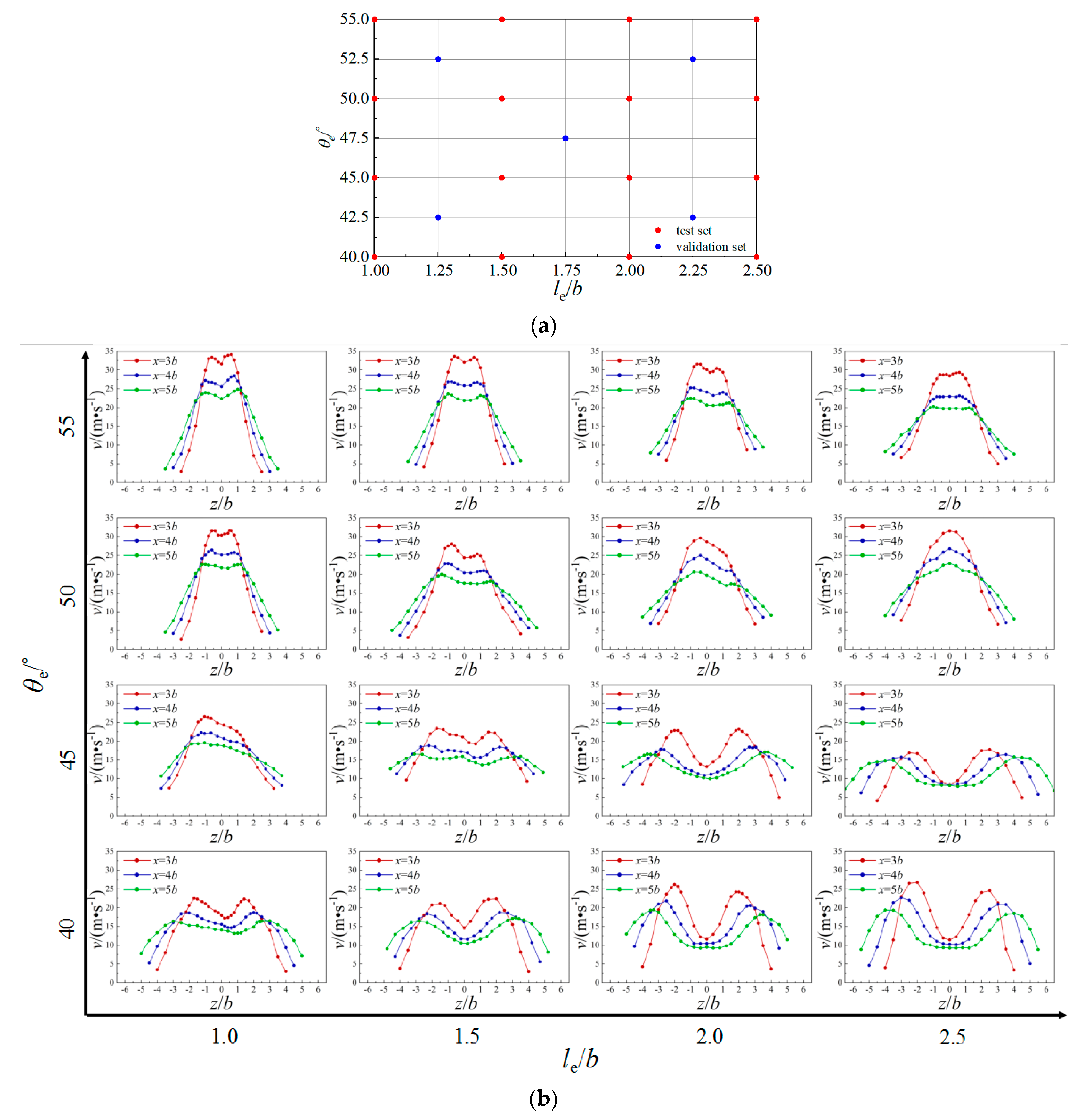
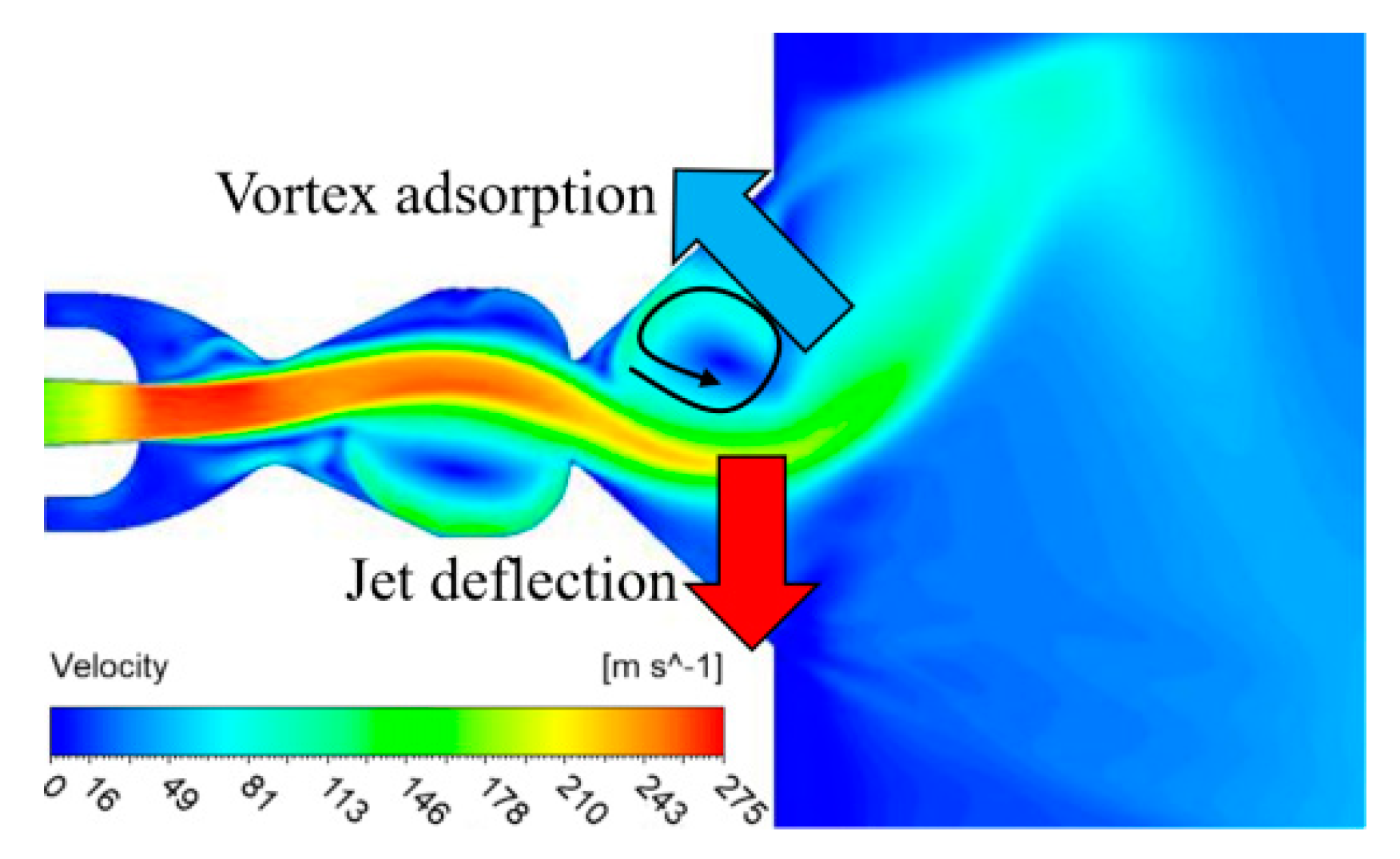
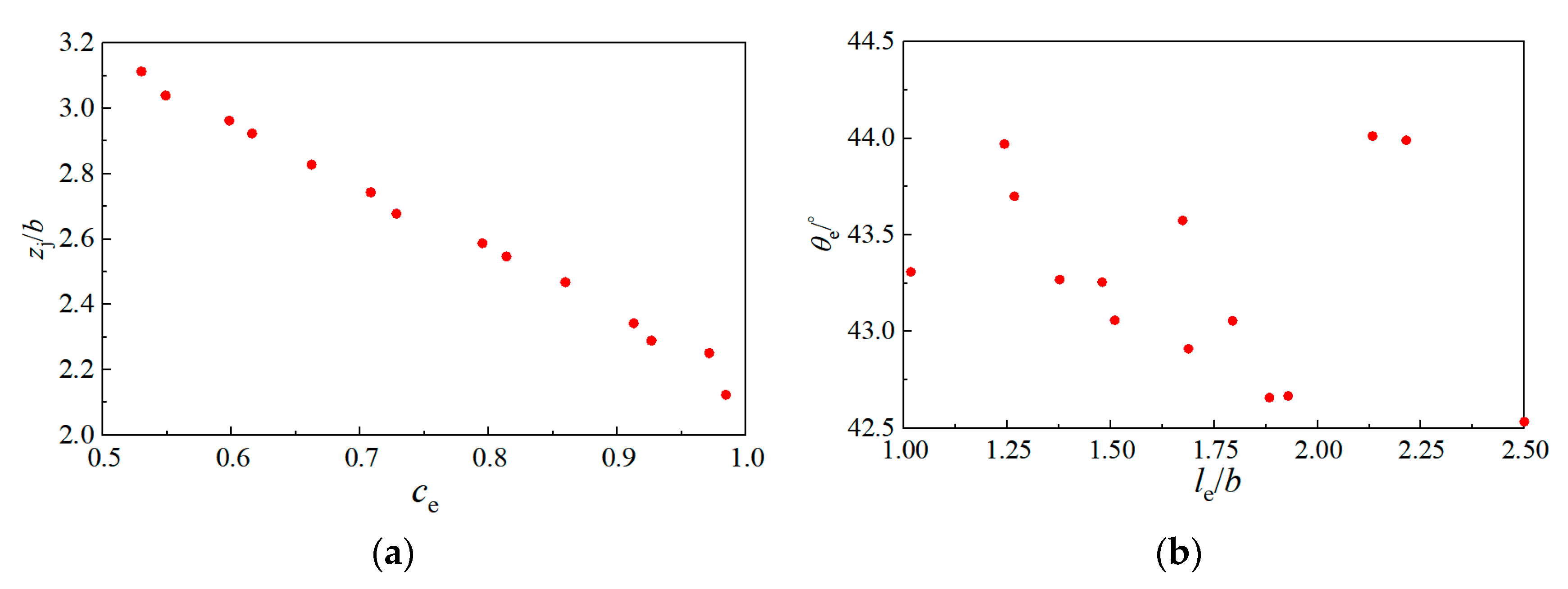
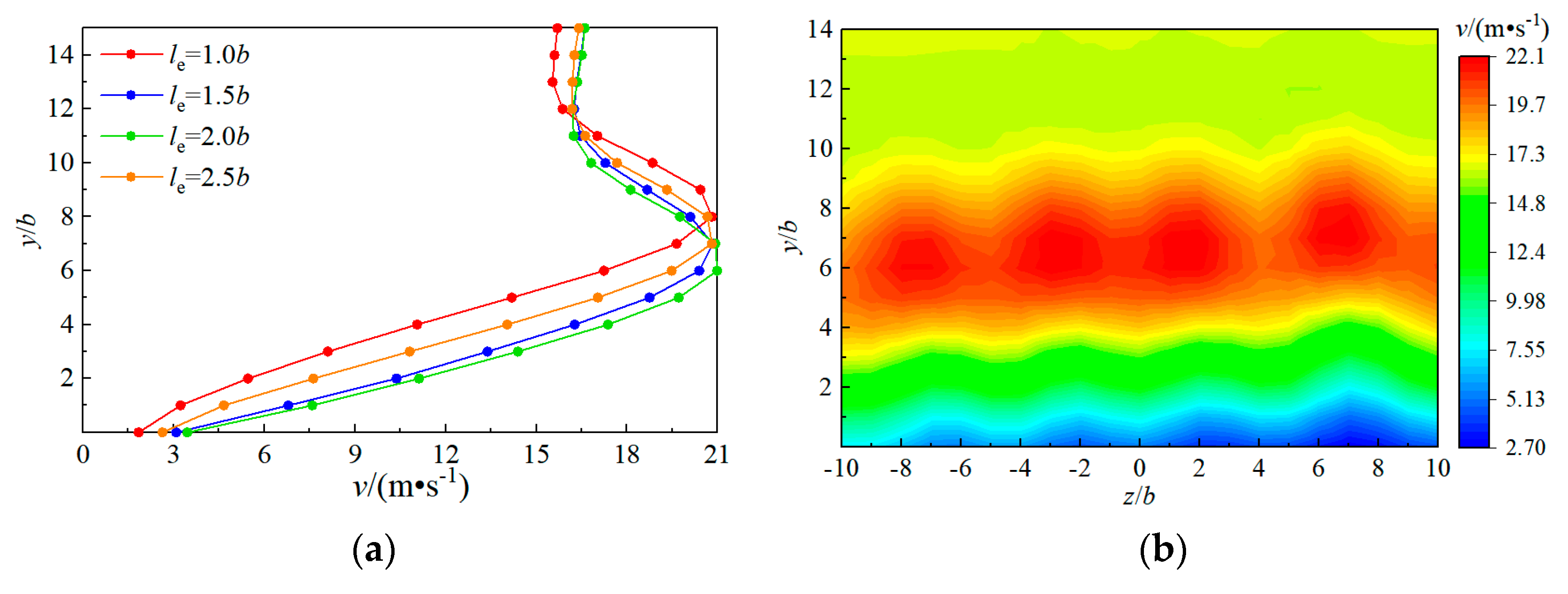
5.3. Effect of the Length of the Expansion Section

When the actuator arrangement distance is small (Δz = 5b), the jet only needs to sweep a small range to cover the whole flap. Therefore, z_j does not need to be too large, and c_e can be increased, which is conducive to improving the control effect. We determined the combination of c_e and z_j that was favorable for separation flow control by changing l_e. The experimental results are as shown in Figure 25. The control effects of l_e = 1.5b and l_e = 2.0b are close to each other (l_e = 2.0b is slightly better), and both are better than the control effects of l_e = 1.0b and l_e = 2.5b. This shows that a large c_e but a small z_j (l_e = 1.0b) or a small c_e but a large z_j (l_e = 2.5b) are not favorable for separation control, and only by coordinating them (l_e = 1.5b~2.0b) can a better control effect be achieved.

From the optimal solution set of the expansion section, ce = 0.8 and z_j = ±2.6b for l_e = 1.5b, which indicates that the sweeping uniformity of the jet is better. As c_e = 0.6 and z_j = ±3.0b for l_e = 2.0b, although the sweeping uniformity of the jet is poor, but a large sweeping range makes up for the shortfall, so l_e should be taken in the range from 1.5b to 2.0b. If the x-direction distance of the AFC module is sufficient, l_e = 2.0b should be chosen. The final optimal actuator parameters are as follows: h_m = 4.35b, l_m = 5.6b, θ_e = 43°, l_e = 2.0b and Δz = 5b.

6. Conclusions

In this study, the external flow velocity distribution of actuators was obtained through hot-wire measurement, and the effects of the geometric parameters on the velocity distribution were analyzed. The modal decomposition of the velocity distribution was carried out using the PCA method, and the influence of each order of modals on the sweeping uniformity and range of the jet was analyzed. The modal-based actuator evaluation parameters were established to complete the optimization of the actuator. The control effect of the optimized actuator on the wing was verified, and the optimal arrangement parameters were obtained. The main conclusions are as follows:

The external flow velocity distribution of actuators has three patterns: unimodal, broad and bimodal. The unimodal pattern indicates that the jet sweeping range is small, the bimodal pattern indicates that the jet is not sweeping uniformly, and the board pattern indicates that the jet is sweeping uniformly and sweeping range is large. Reducing the length of the mixing section and expansion section will transform the velocity distribution pattern to a unimodal distribution; while reducing the height of the mixing section and the expansion angle of the expansion section transforms the velocity distribution pattern to a bimodal distribution.

The modal-based actuator evaluation parameters are applicable for any velocity distribution pattern. The pattern of the modal affects the sweeping uniformity of the jet, and the distance of the modal peaks affects the jet sweeping range. If the modal is a unimodal distribution, it only affects the velocity in the middle of the mean flow field; if the modal is a multimodal distribution, the peak-valley value affects the velocity difference between the two sides and the middle of the mean flow field, and the larger the peaks distance of the modal, the greater the influence of the modal on the jet sweeping range.

The optimal solution sets of the mixing and expansion sections show that the jet sweeping uniformity and sweeping range are negatively correlated, which means that the increase in the jet sweeping uniformity must be accompanied by a decrease in the jet sweeping range. However, when the degree of jet sweeping uniformity is certain, the jet sweeping range in the optimization result of the expansion section is larger than that of the mixing section. Therefore, the mixing section should be selected to ensure uniform jet sweeping, and the jet sweeping range should be increased by optimizing the expansion section.

The influence of the actuator arrangement distance and jet sweeping characteristics on the control effect were analyzed according to the measurement results of the wing wake. The control effect is best when the actuator arrangement distance is comparable to the jet sweeping range. Excessive sweeping uniformity of the jet (a small sweeping range) or an excessive sweeping range (poor sweeping uniformity) is not conducive to separation control, and both have to be coordinated in order to achieve the optimal control effect.

References

1. Liu, R.; Bai, J.Q.; Qiu, Y.S.; Gao, G.Z. Effects of Geometrical Parameters of Internal Blown Flap and Its Optimal Design. J. Northwestern Polytech. Univ. 2020, 38, 58–67. [Google Scholar] [CrossRef]
2. Zha, G.; Paxton, C.; Conley, C.A. Effect of Injection Slot Size on The Performance of Coflow Jet Airfoil. J. Aircr. 2006, 43, 987–995. [Google Scholar] [CrossRef]
3. Liu, Z.Y.; Luo, Z.B.; Yuan, X.X.; Tu, G.H. Review of controlling flow separation over airfoils with periodic excitation. Adv. Mech. 2020, 50, 202007. [Google Scholar]
4. Luo, Z.B.; Xia, Z.X.; Deng, X. Research progress of dual synthetic jets and its flow control technology. Acta Aerodyn. Sin. 2017, 35, 252–264. [Google Scholar]
5. Sun, F.P.; Lin, R.S.; Haas, M. Air flow control by fluidic diverter for low NOx jet engine combustion. In Proceedings of the 1st Flow Control Conference, Reston, VA, USA, 24–26 June 2002. [Google Scholar] [CrossRef]
6. Guyot, D.; Bobusch, B.; Paschereit, C.O. Active combustion control using a fluidic oscillator for asymmetric fuel flow modulation. In Proceedings of the 44th AIAA/ASME/SAE/ASEE Joint Propulsion Conference & Exhibit, Reston, VA, USA, 21–23 July 2008. [Google Scholar] [CrossRef]
7. Li, Z.Y.; Liu, Y.D.; Zhou, W.W. Lift augmentation potential of the circulation control wing driven by sweeping jets. AIAA J. 2022, 60, 4677–4698. [Google Scholar] [CrossRef]
8. Dandois, J.; Verbeke, C.; Ternoy, F. Performance enhancement of a vertical tail model with sweeping jets. AIAA J. 2020, 58, 5202–5215. [Google Scholar] [CrossRef]
9. Kim, S.H. Effects of installation location of fluidic oscillators on aerodynamic performance of an airfoil. Aerosp. Sci. Technol. 2020, 99, 105735. [Google Scholar] [CrossRef]
10. Kara, K.; Kim, D.; Morris, P.J. Flow-separation control using sweeping jet actuator. AIAA J. 2018, 56, 4604–4613. [Google Scholar] [CrossRef]
11. Koklu, M.; Owens, L.R. Comparison of sweeping jet actuators with different flow-control techniques for flow-separation control. AIAA J. 2017, 55, 848–860. [Google Scholar] [CrossRef]
12. Song, J.S. Active flow control in an S-shaped duct at Mach 0.4 using sweeping jet actuators. Exp. Therm. Fluid Sci. 2022, 138, 110699. [Google Scholar] [CrossRef]
13. Schmidt, H.J.; Woszidlo, R.; Nayeri, C.N. Drag reduction on a rectangular bluff body with base flaps and fluidic oscillators. Exp. Fluids 2015, 56, 151. [Google Scholar] [CrossRef]
14. Veerasamy, D.; Tajik, A.R.; Pastur, L. Effect of base blowing by a large-scale fluidic oscillator on the bistable wake behind a flat-back Ahmed body. Phys. Fluids 2022, 34, 035115. [Google Scholar] [CrossRef]
15. Kim, M. Experimental study on heat transfer and flow structures of feedback-free sweeping jet impinging on a flat surface. Int. J. Heat Mass Transf. 2020, 159, 120085. [Google Scholar] [CrossRef]
16. Spens, A.; Bons, J.P. Experimental investigation of synchronized sweeping jets for film cooling application. In Proceedings of the AIAA Scitech 2021 Forum, Reston, VA, USA, 11–15 January 2021. [Google Scholar] [CrossRef]
17. Zhou, W.W.; Wang, K.C.; Yuan, T.J. Spatiotemporal distributions of sweeping jet film cooling with a compact geometry. Phys. Fluids 2022, 34, 025113. [Google Scholar] [CrossRef]
18. Pack, L.G.; Koklu, M. Active flow control using sweeping jet actuators on a semi-span wing model. In Proceedings of the 54th AIAA Aerospace Sciences Meeting, San Diego, CA, USA, 4–8 January 2016. [Google Scholar] [CrossRef]
19. Slupski, B.J.; Kara, K. Separated flow control over NACA 0015 airfoil using sweeping jet actuator. In Proceedings of the 35th AIAA Applied Aerodynamics Conference, Denver, CO, USA, 5–9 June 2017. [Google Scholar] [CrossRef]
20. Tewes, P.; Taubert, L.; Wygnanski, I. On the use of sweeping jets to augment the lift of a λ-wing. In Proceedings of the 28th AIAA Applied Aerodynamics Conference, Chicago, IL, USA, 28 June–1 July 2010. [Google Scholar] [CrossRef]
21. Jones, G.S.; Milholen, W.E.; Chan, D.T. A sweeping jet application on a high Reynolds number semispan supercritical wing configuration. In Proceedings of the 35th AIAA Applied Aerodynamics Conference, Denver, CO, USA, 5–9 June 2017. [Google Scholar] [CrossRef]
22. Spens, A.; Pisano, A.P.; Bons, J.P. Leading-Edge Active Flow Control Enabled by Curved Fluidic Oscillators. AIAA J. 2023, 61, 1675–1686. [Google Scholar] [CrossRef]
23. Seele, R.; Graff, E.; Lin, J. Performance Enhancement of a Vertical Tail Model with Sweeping Jet Actuators. In Proceedings of the 51st AIAA Aerospace Sciences Meeting Including the New Horizons Forum and Aerospace Exposition, Grapevine, TX, USA, 7–10 January 2013. [Google Scholar] [CrossRef]
24. Whalen, E.A.; Lacy, D.S.; Lin, J.C. Performance enhancement of a full-scale vertical tail model equipped with active flow control. In Proceedings of the 53rd AIAA Aerospace Sciences Meeting, Kissimmee, FL, USA, 5–9 January 2015. [Google Scholar] [CrossRef]
25. Andino, M.Y.; Lin, J.C.; Washburn, A.E. Flow separation control on a full-scale vertical tail model using sweeping jet actuators. In Proceedings of the 53rd AIAA Aerospace Sciences Meeting, Kissimmee, FL, USA, 5–9 January 2015. [Google Scholar] [CrossRef]
26. Vatsa, V.N.; Duda, B.M.; Lin, J.C. Numerical simulation of a simplified high-lift CRM configuration embedded with fluidic actuators. In Proceedings of the 2018 Applied Aerodynamics Conference, Atlanta, GA, USA, 25–29 June 2018. [Google Scholar] [CrossRef]
27. Lin, J.C.; Pack, L.G.; Hannon, J. Wind tunnel testing of active flow control on the high lift common research model. In Proceedings of the AIAA Aviation 2019 Forum, Dallas, TX, USA, 17–21 June 2019. [Google Scholar] [CrossRef]
28. Pack, L.G.; Lin, J.C.; Hannon, J. Sweeping jet flow control on the simplified high-lift version of the common research model. In Proceedings of the AIAA Aviation 2019 Forum, Dallas, TX, USA, 17–21 June 2019. [Google Scholar] [CrossRef]
29. Vatsa, V.N.; Lin, J.C.; Pack, L.G. CFD and experimental data comparisons for conventional and AFC-enabled CRM high-lift configurations (invited). In Proceedings of the AIAA AVIATION 2020 Forum, Virtual Event, 15–19 June 2020. [Google Scholar] [CrossRef]
30. Schloesser, P.; Meyer, M.; Schueller, M. Fluidic actuators for separation control at the engine/wing junction. Aircr. Eng. Aerosp. Technol. 2017, 89, 709–718. [Google Scholar] [CrossRef]
31. Ganesh, R.G.; Raghu, S. Cavity Resonance Suppression Using Miniature Fluidic Oscillators. AIAA J. 2004, 42, 2608–2611. [Google Scholar]
32. Brayh, C. Cold Weather Fluidic Fan Spray Devices and Method. U.S. Patent 4463904, 7 August 1984. [Google Scholar]
33. Stouffer, R.D. Liquid Oscillator Device. U.S. Patent 4508267, 2 April 1985. [Google Scholar]
34. Sun, Q.X.; Wang, W.B.; Huang, Y. Key factors affecting the separation control effect of oscillating jets. Acta Aerodyn. Sin. 2023, 41, 56–67. [Google Scholar]
35. Jing, Y.U.; Jiang, A.; Liang, L.I.U.; Xiaojun, W.U.; Yewei, G.U.I.; Shenshen, L.I.U. PCA aerodynamic geometry parametrization method. Acta Aeronaut. Et Astronaut. Sin. 2024, 45, 129125. [Google Scholar]
36. Bobusch, B.C.; Woszidlo, R.; Bergada, J.M. Experimental study of the internal flow structures inside a fluidic oscillator. Exp. Fluids 2013, 54, 1559. [Google Scholar] [CrossRef]
37. Bobusch, B.C.; Woszidlo, R.; Kruger, O. Numerical Investigations on Geometric Parameters Affecting the Oscillation Properties of a Fluidic Oscillator. In Proceedings of the 21st AIAA Computational Fluid Dynamics Conference, San Diego, CA, USA, 24–27 June 2013. [Google Scholar]
Figure 1. Oscillating jet actuator.
Aerospace 11 00916 g001
Figure 2. Internal flow structure of the actuator: (a) t = 0T, (b) t = 1/6T, (c) t = 1/3T, (d) t = 1/2T.
Aerospace 11 00916 g002
Figure 3. Wing model: (a) airfoil, (b) plexiglass panel, (c) wing for mounting panels.
Aerospace 11 00916 g003
Figure 4. Hot-wire scanning plane: (a) monitoring lines for velocity distribution measurement, (b) monitoring surface for wing wake measurement.
Aerospace 11 00916 g004
Figure 5. Arrangement of the equipment in the wind tunnel.
Aerospace 11 00916 g005
Figure 6. Typical actuator control characteristics in the literature: (a) geometry of the actuator, (b) flow field characteristics outside the actuator, (c) deflection flap separation flow control effect [34].
Aerospace 11 00916 g006
Figure 7. Optimization flow chart.
Aerospace 11 00916 g007
Figure 8. Samples and test results: (a) training and validation set distributions; (b) mixing section test results.
Aerospace 11 00916 g008
Figure 9. Flow field inside the mixing section [34]: (a) hm = 4.5b lm = 5.25b. (b) hm = 4.5b lm = 6.5b.
Aerospace 11 00916 g009
Figure 10. Contribution ratio.
Aerospace 11 00916 g010
Figure 11. PCA results: (a) modal1; (b) modal2; (c) modal3; (d) modal4.
Aerospace 11 00916 g011aAerospace 11 00916 g011b
Figure 12. Reconfiguration results: (a) hm = 4.5b lm = 5b; (b) hm = 3.5b lm = 5b; (c) hm = 4.0b lm = 6.5b.
Aerospace 11 00916 g012
Figure 13. Principal component surrogate models: (a) PC1, (b) PC2, (c) PC3.
Aerospace 11 00916 g013
Figure 14. Surrogate models of evaluation parameters: (a) ce; (b) zj.
Aerospace 11 00916 g014
Figure 15. Optimization results of mixing section: (a) pareto front; (b) optimized variable.
Aerospace 11 00916 g015
Figure 16. Optimal configuration: (a) optimal mixing section parameters, (b) optimal configuration validation.
Aerospace 11 00916 g016
Figure 17. Samples and test results: (a) training and validation set distributions; (b) expansion section test results.
Aerospace 11 00916 g017
Figure 18. Flow field in the expansion section [34].
Aerospace 11 00916 g018
Figure 19. PCA results: (a) contribution ratio; (b) model1; (c) model2; (d) mean flow field.
Aerospace 11 00916 g019
Figure 20. PCA surrogate models: (a) PC1; (b) PC2; (c) ce; (d) zj.
Aerospace 11 00916 g020
Figure 21. Optimization results of the expansion section: (a) pareto front, (b) optimized variable values.
Aerospace 11 00916 g021
Figure 22. Optimization result: (a) optimal actuator model; (b) variation of jet oscillation frequency with flow rate.
Aerospace 11 00916 g022
Figure 23. Flow field over wing at different Cμ: (a) velocity distribution on monitoring surface (Cμ = 0); (b) velocity distribution on monitoring surface (Cμ = 0.03); (c) spanwise averaged wake.
Aerospace 11 00916 g023
Figure 24. Flow field over wing for different actuator arrangement distance: (a) spanwise averaged wake; (b) velocity distribution on monitoring surface (Δz = 8b); (c) velocity distribution on monitoring surface (Δz = 5b).
Aerospace 11 00916 g024
Figure 25. Flow field over wing at different le: (a) spanwise averaged wake; (b) velocity distribution on monitoring surface (le = 2.0b).
Aerospace 11 00916 g025