The Influence of Ice Accretion on the Thermodynamic Performance of a Scientific Balloon: A Simulation Study

Abstract

A scientific balloon is the ideal platform for carrying out long-duration missions for scientific research in the stratosphere. However, when a scientific balloon ascends through icy clouds and reaches supercooled droplets, there is a risk of ice accretion on the balloon’s surface. Ice accretion on the balloon can threaten flight safety and the accomplishment of missions and can even result in disastrous accidents. A comprehensive simulation platform was developed to simulate the influence of ice accretion on the thermodynamic performance of a scientific balloon to provide quantitative data support for balloon design and flight operations. The simulation platform consisted of two parts: one based on ANSYS software to solve the accretion model and the other a program developed with MATLAB software to solve the thermodynamic model. The results suggest that, in certain cloud environments, there is a risk of ice accretion on a balloon’s surface; the extra ice mass added to the balloon may prevent it from ascending through icy clouds and instead keep it floating at the base of these clouds.

1. Introduction

A scientific balloon is the ideal platform for carrying out long-duration missions for scientific research in the stratosphere [1,2,3]. When a scientific balloon ascends through icy clouds and reaches supercooled droplets, there is a risk of ice accretion on the balloon’s surface. Ice accretion on the balloon’s surface will add extra mass to the balloon and break its buoyancy–gravity balance. Thus, ice accretion may deteriorate the balloon’s thermodynamic performance, threaten flight safety and the accomplishment of designed missions, and even result in disastrous accidents. A comprehensive understanding of the influence of ice accretion on the thermodynamic performance of scientific balloons in the ascension process is vitally important for designers and flight operators. The present study investigated the influence of ice accretion on thermodynamic performance to provide quantitative data support for scientific balloon design and flight operations.

The influence of ice accretion on the thermodynamic performance of a scientific balloon relates to three aspects: (1) cloud radiation properties; (2) ice accretion models; and (3) thermodynamic models with cloud modification. The cloud environment around a scientific balloon is described in Figure 1.

Figure 1 suggests that in the whole-flight profile, the thermal environment is modified by clouds. During the ascent and descent stages, the balloon can encounter clouds and be influenced by both radiation-related thermal environment changes and ice accretion. In the floating stage, the balloon can be influenced by infrared radiation.

The following briefly discusses the state-of-the-art of investigations into thermodynamic models of scientific balloons. Kreith and Kreider constructed a thermodynamic model that can calculate the average temperature of a balloon envelope and lift gas and predict the balloon’s trajectory; this model is considered the starting point for subsequent research. Farley et al. established a thermodynamic model for scientific balloons that can predict balloon ascent trajectories both vertically and horizontally [4]. Dai et al. investigated the thermal performance of scientific balloons by dividing the envelope into small elements and building a thermal model for each element; in this way, the thermal model can determine the balloon’s temperature distribution with higher accuracy [5]. Louchev et al. developed a steady-state thermal model for hot air balloons; the thermal model can calculate the steady-state temperature distribution of a balloon envelope and the average temperature of the lift gas under different conditions [6]. Xia et al. established a transient numerical thermal model that can calculate the temperature distribution of a balloon envelope in floating conditions [7]. Wang and Yang proposed a transient numerical model that can evaluate the temperature distribution across the balloon envelope and investigate the natural convection heat transfer between helium gas and the balloon envelope inside the balloon [8]. Liu et al. proposed a novel numerical model to investigate the thermodynamic performance of scientific balloons [9], consisting of a dynamic model and a thermal model. The dynamic model is numerically solved with a computer program developed with MATLAB/Simulink to calculate the velocity and trajectory, and the thermal model is solved with the Fluent program to determine the balloon’s film temperature distribution and the inner helium gas velocity and temperature field.

The progress made in this topic is briefly summarized below. Ice accretion on scientific balloons shares much in common with that on aircraft, so research on aircraft icing may provide a reference for scientific balloons. Messinger constructed a simple but effective two-dimensional numerical model to calculate the icing performance of an airfoil [10]; the model was assumed to be quasi-steady and combined the conservation of mass and energy. This model was a pioneering work in the ice-accretion-modeling field; from this starting point, numerical simulations of aircraft icing performance have considerably progressed and been widely used, facilitated by rapid developments in computer capability and CFD theories. Later, the icing analysis model advanced from two dimensions to three dimensions.

Based on the classical Messinger model, Shen et al. considered the effect of runback water and developed a three-dimensional ice accretion model to calculate ice shapes at the engine inlet [11]. Based on the Eulerian two-phase flow theory and extended heat transfer fluxes, Cao et al. proposed a three-dimensional model capable of numerically simulating ice accretion on an aircraft’s wing [12]. Liu proposed a three-dimensional ice accretion mode to simulate the icing performance of a stratospheric airship when it flies through icy clouds and encounters supercooled droplets in the ascending process [13]. The results suggest that ice will accrete on the windward surface of the airship under certain conditions; ice accretion will change the aerodynamic performance and break the lift and gravity balance of the airship, seriously deteriorating the flight performance of the airship. Several icing analysis codes have been developed [14,15], including the TRAJICE code by DRA, the ONERA code by France, the IMPIN3D code by the Italian Aerospace Research Center, the LEWICE code developed by the NASA Glenn Research Center, and the FENSAP-ICE code developed by McGill University in Canada.

The remainder of this study is organized as follows. Firstly, we present a brief introduction regarding the importance of this study and the state of the art in this research. Secondly, we introduce theory analyses and a mathematical description of cloud radiation properties, the ice accretion model, and a thermodynamic model with cloud modification. Thirdly, we analyze the method and validate the ice accretion and thermodynamic models. Fourthly, the ice accretion performance is numerically analyzed, and we further investigate the influence of ice accretion. Finally, conclusions are drawn from the analysis.

2. Theoretical Model

2.1. Cloud Radiation Properties

Clouds influence the thermal radiation environment of scientific balloons by transmitting radiation heat, reflecting radiation heat, and emitting infrared radiation heat. The transmittance, reflectance, and emittance of clouds are closely related to their optical thickness, which is determined by their height, appearance, thickness, liquid droplet phase, water content, average droplet diameter, etc.

1.

Optical thickness of clouds

When the thermal radiation wavelength is smaller than 4 μm, the optical thickness of a cloud (${\tau }_{\lambda }$) can be calculated using the following equation [16]:

$${\tau }_{\lambda }=LWP(a_1+{\displaystyle \frac{a_2}{r_{\mathrm{e}}}})$$

(1)

Here, $LWP$ is the total water content of the cloud from the bottom to the top, which can be calculated as follows:

$$LWP={\displaystyle {\int }_{H_{\mathrm{cloudbase}}}^{H_{\mathrm{cloudtop}}}LWCdz}$$

(2)

Here, $a_i$ is the curve-fitting constant; $r_{\mathrm{e}}$ is the mean droplet diameter; $LWC$ is the level of water content per cubic meter; and $H_{\mathrm{cloudbase}}$ and $H_{\mathrm{cloudtop}}$ are the altitude of the cloud and its top, respectively.

When the thermal radiation wavelength is larger than 4 μm, the optical thickness of the cloud (${\tau }_{\lambda }$) can be calculated using the following equation [17]:

$${\tau }_{\lambda }=LWC\cdot z\cdot {\phi }_{\lambda }$$

(3)

Here, $b_i$, $c_i$, and $d_i$ are the curve-fitting constants, and $z$ is the thickness of the cloud.

${\phi }_{\lambda }$ can be calculated as follows:

$${\phi }_{\lambda }=b_1+b_2{r}_{\mathrm{e}}+b_3/r_{\mathrm{e}}+b_4/r_{\mathrm{e}}^2+b_5/r_{\mathrm{e}}^3$$

(4)

2.

Transmittance of the cloud

The transmittance of the cloud (${\tau }_{\mathrm{c}}$) can be calculated as follows [18]:

$${\tau }_{\mathrm{c}}={\displaystyle \frac{4u}{R}}$$

(5)

Here, the parameters $u$ and $R$ can be calculated using the following equations:

$$u^2={\displaystyle \frac{1-{\omega }_0+2\beta \left({\mu }_0\right){\omega }_0}{1-{\omega }_0}}$$

(6)

$${\tau }_{\mathrm{eff}}={\displaystyle \frac{{\left\{\left(1-{\omega }_0\right)\left[1-{\omega }_0+2\beta \left({\mu }_0\right){\omega }_0\right]\right\}}^{1/2}{\tau }_{\lambda }}{{\mu }_0}}$$

(7)

$$R={\left(u+1\right)}^2\exp \left({\tau }_{\mathrm{eff}}\right)-{\left(u-1\right)}^2\exp \left(-{\tau }_{\mathrm{eff}}\right)$$

(8)

3.

Cloud reflectance

The cloud reflectance (${\rho }_{\mathrm{c}}$) can be calculated as follows [19]:

$${\rho }_{\mathrm{c}}={\displaystyle \frac{{\rho }^{\infty }[\exp (\delta {\tau }_{\lambda })-\exp (-\delta {\tau }_{\lambda })]}{[\exp (\delta {\tau }_{\lambda })-{\rho }^{\infty }\exp (-\delta {\tau }_{\lambda })]}}$$

(9)

Here, the parameters $\delta$ and ${\rho }^{\infty }$ can be calculated using the following equations:

$$\delta =2\sqrt{(1-{\omega }_0)(1-{\omega }_0{g}_0)}$$

(10)

$${\rho }^{\infty }={\displaystyle \frac{\sqrt{1-{\omega }_0{g}_0}-\sqrt{1-{\omega }_0}}{\sqrt{1-{\omega }_0{g}_0}+\sqrt{1-{\omega }_0}}}$$

(11)

4.

Cloud emittance

A cloud can be treated as a gray body; cloud emittance (${\epsilon }_{\mathrm{c}}$) can be calculated as follows [20]:

$${\epsilon }_{\mathrm{c}}=1-\alpha \cdot \exp \left(-\beta \cdot LWC\cdot z\right)$$

(12)

Here, $\alpha$ and $\beta$ are constants.

2.2. Ice Accretion Model

Ice accretion on a balloon’s surface can be divided into three sequential processes: (1) Super-cooled droplets flow around the balloon; (2) the super-cooled droplets impinge on the windward part of the balloon, and some of the droplets accumulate on the surface, forming a thin water film; (3) the thin water film changes phase into ice through heat and mass transfer.

Analyzing ice accretion on a balloon’s surface comprises three modules in accordance with the above-mentioned processes: the thermal and airflow module, the droplet impingement module, and the ice accretion module. The relationship between the three modules is depicted in Figure 2.

Resolving the thermal and icing problems in three dimensions proceeds as follows. Firstly, the thermal and airflow module calculates the thermal and airflow distribution of the balloon. Secondly, the droplet impingement module imports the mesh and dry airflow results from the thermal and airflow module and computes the water collection efficiency and thin film flow on the balloon’s surface. Thirdly, the ice accretion module imports the balloon’s temperature and water collection efficiency to calculate the ice accreted on the balloon’s surface.

A detailed description of the transient mass, momentum, and energy-governing equations of the thermal and airflow module, the droplet impingement module, and the ice accretion module can be found in [13].

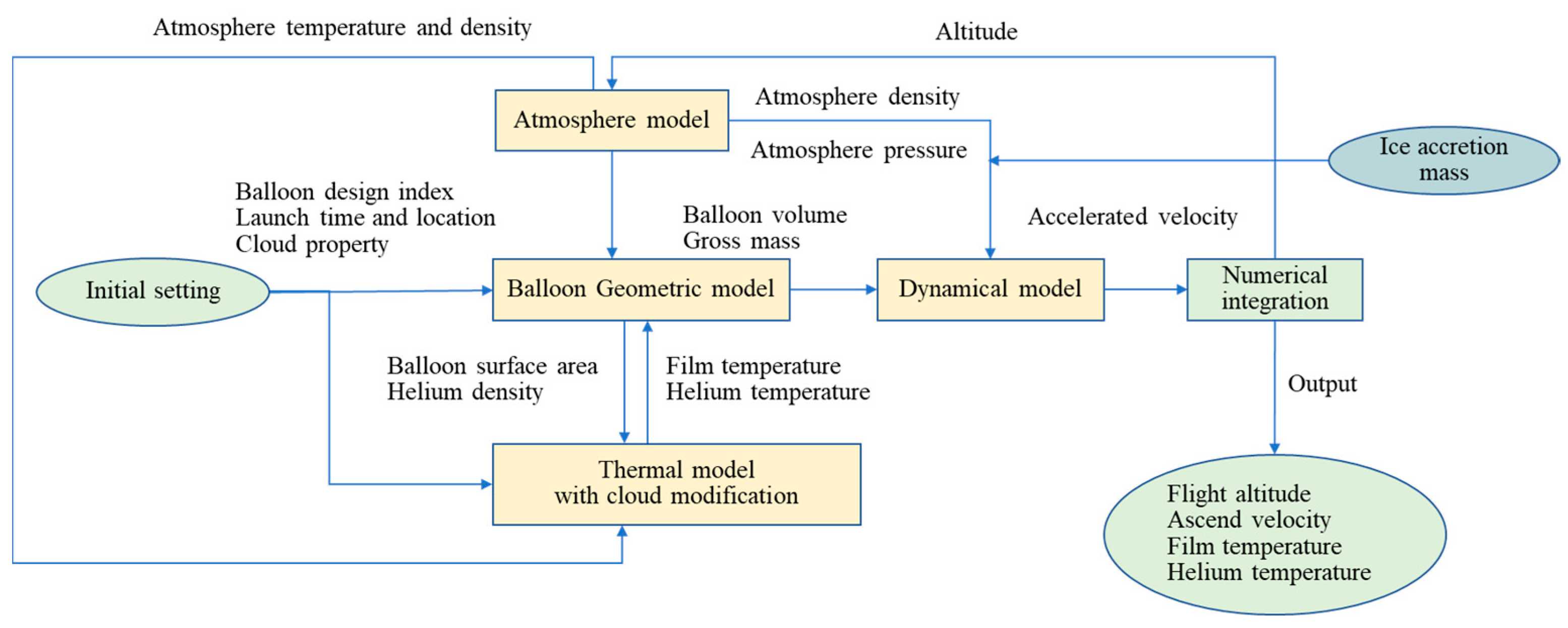
2.3. Thermodynamic Model with Cloud Modification

2.3.1. Geometry of the Balloon

The balloon volume ($V$) is equal to the helium volume ($V_{\mathrm{He}}$) inside the balloon, which obeys the ideal gas law [4].

$$V=V_{\mathrm{He}}=m_{\mathrm{He}}\cdot R_{\mathrm{He}}\cdot T_{\mathrm{He}}/P_{\mathrm{He}}$$

(13)

Here, $R_{\mathrm{He}}$ is the gas constant of helium; $m_{\mathrm{He}}$, $T_{\mathrm{He}}$, and $P_{\mathrm{He}}$ are the mass, temperature, and pressure of helium inside the balloon, respectively.

The balloon diameter can be calculated as follows [4]:

$$d=1.424\cdot V^{1/3}$$

(14)

A balloon surface area with a pumpkin shape can be calculated as follows:

$$A_{\mathrm{surf}}\approx 5.3\cdot V^{2/3}$$

(15)

The projected area of the top of the balloon can be calculated as follows:

$$A_{\mathrm{top}}=\pi /4\cdot d^2$$

(16)

The projected area of the balloon’s illumination ($A_{\mathrm{projected}}$) varies with the solar elevation angle ($h$) and can be calculated as follows:

$$A_{\mathrm{projected}}=A_{\mathrm{top}}\cdot [0.8219+0.1781\cos (\pi -2h)]$$

(17)

The volume of the balloon expands as it ascends; when it approaches its designated float altitude, the volume increases to its maximum state. Differential pressure may arise between the inside and outside of the balloon; in this situation, the helium gas is vented through a valve to maintain acceptable differential pressure.

The velocity flow ($Velocit{y}_{flow}$) of helium through the valve relates to the differential pressure ($\Delta P_{valve}$) across the valve interface, the density of the helium (${\rho }_{He}$), and the discharge coefficient ($C_{disch\arg e}$).

$$Velocit{y}_{flow}=C_{disch\arg e}·{(2\Delta P_{valve}/{\rho }_{He})}^{0.5}$$

(18)

This leads to the mass differential equation of helium inside the balloon:

$${\displaystyle \frac{d{m}_{He}}{dt}}=-C{A}_{valve}{(2\Delta P_{valve}·{\rho }_{He})}^{0.5}$$

(19)

Here, $A_{valve}$ is the area of the valve cross-section. The discharge coefficient ($C_{disch\arg e}$) is approximately 0.6 for a sharp-edged hole [4].

2.3.2. Thermal Environment of the Balloon

The scientific balloon’s modified thermal environment when it is partially inflated and inside the cloud in the ascending state is depicted in Figure 3.

Figure 3 shows that, when the scientific balloon is inside the cloud, direct solar radiation, solar scatter radiation, and atmospheric infrared radiation will be transmitted to the cloud and attenuated by it before the balloon reaches it. Solar albedo radiation will be transmitted to the cloud twice and attenuated by it twice before the balloon reaches it. In this situation, convection heat transfers between the balloon’s outer surface and atmosphere because of the temperature difference. If super-cooled droplets are in the cloud, ice may accrete on the balloon’s surface.

The balloon film and helium thermal models with cloud modification are described as follows.

1.

Balloon film thermal model

The temperature change rate of the balloon film can be derived from the transient energy balance equation [5]:

$$\begin{array}{l}{\displaystyle \frac{d{T}_{\mathrm{film}}}{dt}}=[(Q_{\mathrm{s}-\mathrm{direct}-\mathrm{cm}}+Q_{\mathrm{s}-\mathrm{scatter}-\mathrm{cm}}+Q_{\mathrm{s}-\mathrm{albedo}-\mathrm{cm}}+Q_{\mathrm{s}-\mathrm{cloud}}+Q_{\mathrm{IR}-\mathrm{atm}-\mathrm{cm}}+Q_{\mathrm{IR}-\mathrm{cloud}}+Q_{\mathrm{IR}-\mathrm{earth}-\mathrm{cm}}+Q_{\mathrm{IR}-\mathrm{film}-\mathrm{ext}}+Q_{\mathrm{IR}-\mathrm{film}-\mathrm{int}}\\ +Q_{\mathrm{Conv}-\mathrm{ext}}+Q_{\mathrm{Conv}-\mathrm{int}})]/(c_{\mathrm{f}}\cdot m_{\mathrm{film}})\end{array}$$

(20)

where $T_{\mathrm{film}}$ is the temperature of the balloon film, $c_{\mathrm{f}}$ is the specific heat of the balloon film material, $m_{\mathrm{film}}$ is the mass of the balloon film, $Q_{\mathrm{s}-\mathrm{direct}-\mathrm{cm}}$ is the absorbed direct solar radiation flux, $Q_{\mathrm{s}-\mathrm{scatter}-\mathrm{cm}}$ is the absorbed atmosphere scattered solar radiation flux, $Q_{\mathrm{s}-\mathrm{albedo}-\mathrm{cm}}$ is the absorbed Earth-surface reflected solar radiation flux, $Q_{\mathrm{s}-\mathrm{cloud}}$ is the absorbed cloud reflected solar radiation flux, $Q_{\mathrm{IR}-\mathrm{atm}-\mathrm{cm}}$ is the absorbed atmosphere infrared radiation flux, $Q_{\mathrm{IR}-\mathrm{cloud}}$ is the absorbed cloud infrared radiation flux, $Q_{\mathrm{IR}-\mathrm{earth}-\mathrm{cm}}$ is the absorbed Earth-surface infrared radiation flux, $Q_{\mathrm{IR}-\mathrm{film}-\mathrm{ext}}$ is the emitted infrared radiation flux of the external balloon film, $Q_{\mathrm{IR}-\mathrm{film}-\mathrm{int}}$ is the absorbed infrared radiation flux of the internal balloon film, $Q_{\mathrm{Conv}-\mathrm{ext}}$ is the net gain of external convective heat transfer flux, and $Q_{\mathrm{Conv}-\mathrm{int}}$ is the net gain of internal convective heat transfer flux.

(1)

Absorbed solar direct radiation flux

The absorbed direct solar radiation flux ($Q_{\mathrm{s}-\mathrm{direct}-\mathrm{cm}}$) of the balloon film can be calculated as follows [5].

$$Q_{\mathrm{s}-\mathrm{direct}-\mathrm{cm}}=I_{\mathrm{s}-\mathrm{direct}-\mathrm{cm}}\cdot A_{\mathrm{projected}}\cdot {\alpha }_{\mathrm{film}}\cdot [1+{\tau }_{\mathrm{film}}\cdot (1+r_{\mathrm{eff}})]$$

(21)

Here, $I_{\mathrm{s}-\mathrm{direct}-\mathrm{cm}}$ represents the solar direct radiation intensity with cloud modification.

$$I_{\mathrm{s}-\mathrm{direct}-\mathrm{cm}}=\left\{\begin{array}{l}{I}_{\mathrm{s}-\mathrm{direct}}\cdot {\tau }_{\mathrm{c}}\hspace{1em}\hspace{1em} H<H_{\mathrm{cloudbase}}\\ I_{\mathrm{s}-\mathrm{direct}}\cdot {\tau }_{\mathrm{c}-\mathrm{up}}\hspace{1em} H_{\mathrm{cloudbase}}\le H\le H_{\mathrm{cloudtop}}\\ I_{\mathrm{s}-\mathrm{direct}}\hspace{1em}\hspace{1em}\hspace{1em}\hspace{1em}H>H_{\mathrm{cloudtop}}\end{array}\right.$$

(22)

Here, ${\alpha }_{\mathrm{film}}$ and ${\tau }_{\mathrm{film}}$ represent the absorptivity and transmittance of the balloon film for the solar radiation, respectively. $r_{\mathrm{eff}}$ denotes the effective reflectance inside the balloon; a detailed calculation can be found in [5]. $H$ represents the flight altitude of the balloon, and ${\tau }_{\mathrm{c}-\mathrm{up}}$ is the cloud transmittance from the flight altitude of the balloon to the top of the cloud.

(2)

Absorbed solar scatter radiation flux [5]

The absorbed solar scatter radiation flux ($Q_{\mathrm{s}-\mathrm{scatter}-\mathrm{cm}}$) of the balloon film can be calculated as follows.

$$Q_{\mathrm{s}-\mathrm{scatter}-\mathrm{cm}}=I_{\mathrm{s}-\mathrm{scatter}-\mathrm{cm}}\cdot A_{\mathrm{surf}}\cdot {\alpha }_{\mathrm{film}}\cdot [1+{\tau }_{\mathrm{film}}\cdot (1+r_{\mathrm{eff}})]$$

(23)

Here, $I_{\mathrm{s}-\mathrm{scatter}-\mathrm{cm}}$ denotes the solar scatter radiation intensity with cloud modification:

$$I_{\mathrm{s}-\mathrm{scatter}-\mathrm{cm}}=\left\{\begin{array}{l}{I}_{\mathrm{s}-\mathrm{scatter}}\cdot {\tau }_{\mathrm{c}}\hspace{1em}\hspace{1em} H<H_{\mathrm{cloudbase}}\\ I_{\mathrm{s}-\mathrm{scatter}}\cdot {\tau }_{\mathrm{c}-\mathrm{up}}\hspace{1em}{H}_{\mathrm{cloudbase}}\le H\le H_{\mathrm{cloudtop}}\\ I_{\mathrm{s}-\mathrm{scatter}}\hspace{1em}\hspace{1em}\hspace{1em} H>H_{\mathrm{cloudtop}}\end{array}\right.$$

(24)

(3)

Absorbed solar albedo radiation flux

The absorbed solar albedo radiation flux ($Q_{\mathrm{s}-\mathrm{albedo}-\mathrm{cm}}$) of the balloon film can be calculated as follows:

$$Q_{\mathrm{s}-\mathrm{albedo}-\mathrm{cm}}=I_{\mathrm{albedo}-\mathrm{cm}}\cdot A_{\mathrm{surf}}\cdot {\alpha }_{\mathrm{film}}\cdot X_{\mathrm{e}-\mathrm{b}}[1+{\tau }_{\mathrm{film}}\cdot (1+r_{\mathrm{eff}})]$$

(25)

Here, $I_{\mathrm{s}-\mathrm{albedo}-\mathrm{cm}}$ is the solar albedo radiation intensity with cloud modification:

$$I_{\mathrm{s}-\mathrm{albedo}-\mathrm{cm}}=\left\{\begin{array}{l}{I}_{\mathrm{albedo}}\cdot {\tau }_{\mathrm{c}}\hspace{1em}\hspace{1em}\hspace{1em}\hspace{1em}H<H_{\mathrm{cloudbase}}\\ I_{\mathrm{albedo}}\cdot {\tau }_{\mathrm{c}}\cdot {\tau }_{\mathrm{c}-\mathrm{below}}\hspace{1em}{H}_{\mathrm{cloudbase}}\le H\le H_{\mathrm{cloudtop}}\\ I_{\mathrm{albedo}}\cdot {\tau }_{\mathrm{c}}^2\hspace{1em}\hspace{1em}\hspace{1em}\hspace{1em}H>H_{\mathrm{cloudtop}}\end{array}\right.$$

(26)

Here, $X_{\mathrm{e}-\mathrm{b}}$ and ${\tau }_{\mathrm{film}}$ represent the view factor of radiation heat transfer from the balloon to the Earth’s surface; a detailed calculation can be found in [5]. ${\tau }_{\mathrm{c}-\mathrm{below}}$ is the cloud transmittance from the bottom of the cloud to the flight altitude of the balloon.

(4)

Absorbed cloud reflected solar radiation flux

When the balloon is above the cloud, the absorbed solar cloud albedo radiation flux ($Q_{\mathrm{s}-\mathrm{cloud}}$) of the balloon film can be calculated as follows:

$$Q_{\mathrm{s}-\mathrm{cloud}}={\rho }_{\mathrm{c}}(I_{\mathrm{s}-\mathrm{direct}}\cdot \sin h\cdot A_{\mathrm{projected}}+I_{\mathrm{s}-\mathrm{scatter}}\cdot {\displaystyle \frac{1}{2}}{A}_{\mathrm{surf}})\cdot {\alpha }_{\mathrm{film}}[1+{\tau }_{\mathrm{film}}\cdot (1+r_{\mathrm{eff}})]$$

(27)

(5)

Absorbed atmosphere infrared radiation flux

The atmosphere infrared radiation flux ($Q_{\mathrm{IR}-\mathrm{atm}-\mathrm{cm}}$) of the balloon film can be calculated as follows:

$$Q_{\mathrm{IR}-\mathrm{atm}-\mathrm{cm}}=I_{\mathrm{IR}-\mathrm{atm}-\mathrm{cm}}\cdot A_{\mathrm{surf}}\cdot {\alpha }_{\mathrm{film}-\mathrm{IR}}\cdot (1-X_{\mathrm{e}-\mathrm{b}})\cdot [1+{\tau }_{\mathrm{film}-\mathrm{IR}}\cdot (1+r_{\mathrm{eff}})]$$

(28)

Here, $I_{\mathrm{IR}-\mathrm{atm}-\mathrm{cm}}$ is the infrared radiation of the atmosphere with cloud modification:

$$I_{\mathrm{IR}-\mathrm{atm}-\mathrm{cm}}=\left\{\begin{array}{l}{I}_{\mathrm{IR}-\mathrm{atm}}\cdot {\tau }_{\mathrm{c}}\hspace{1em}\hspace{1em} H<H_{\mathrm{cloudbase}}\\ I_{\mathrm{IR}-\mathrm{atm}}\cdot {\tau }_{\mathrm{c}-\mathrm{up}}\hspace{1em} H_{\mathrm{cloudbase}}\le H\le H_{\mathrm{cloudtop}}\\ I_{\mathrm{IR}-\mathrm{atm}}\hspace{1em}\hspace{1em}\hspace{1em}\hspace{1em}H>H_{\mathrm{cloudtop}}\end{array}\right.$$

(29)

(6)

Absorbed cloud infrared radiation flux

The absorbed cloud infrared radiation flux ($Q_{\mathrm{IR}-\mathrm{cloud}}$) of the balloon film can be calculated as follows:

$$Q_{\mathrm{IR}-\mathrm{cloud}}=\sigma \cdot {\epsilon }_{\mathrm{c}}\cdot T_{\mathrm{cloud}}^4\cdot {\displaystyle \frac{1}{2}}{A}_{\mathrm{surf}}\cdot {\alpha }_{\mathrm{film}-\mathrm{IR}}\cdot [1+{\tau }_{\mathrm{film}-\mathrm{IR}}\cdot (1+r_{\mathrm{eff}})]$$

(30)

Here, ${\alpha }_{\mathrm{film}-\mathrm{IR}}$ and ${\tau }_{\mathrm{film}-\mathrm{IR}}$ represent the absorptivity and transmittance of the balloon film for the infrared radiation, respectively. $T_{\mathrm{cloud}}$ denotes the temperature of the cloud.

(7)

Absorbed Earth-surface infrared radiation flux

The absorbed Earth-surface infrared radiation flux ($Q_{\mathrm{IR}-\mathrm{earth}-\mathrm{cm}}$) of the balloon film can be calculated as follows:

$$Q_{\mathrm{IR}-\mathrm{earth}-\mathrm{cm}}=I_{\mathrm{IR}-\mathrm{earth}-\mathrm{cm}}\cdot A_{\mathrm{surf}}\cdot {\alpha }_{\mathrm{film}-\mathrm{IR}}\cdot X_{\mathrm{e}-\mathrm{b}}\cdot [1+{\tau }_{\mathrm{film}-\mathrm{IR}}\cdot (1+r_{\mathrm{eff}})]$$

(31)

(8)

Emitted infrared radiation flux of the external balloon film

The emitted infrared radiation flux of the external balloon film ($Q_{\mathrm{IR}-\mathrm{film}-\mathrm{ext}}$) can be calculated as follows:

$$Q_{\mathrm{IR}-\mathrm{film}-\mathrm{ext}}=-2\sigma \cdot {\epsilon }_{\mathrm{film}}\cdot T_{\mathrm{film}}^4\cdot A_{\mathrm{surf}}$$

(32)

(9)

Absorbed infrared radiation flux of the internal balloon film

The absorbed infrared radiation flux of the internal balloon film ($Q_{\mathrm{IR}-\mathrm{film}-\mathrm{int}}$) can be calculated as follows:

$$Q_{\mathrm{IR}-\mathrm{film}-\mathrm{int}}=\sigma \cdot {\epsilon }_{\mathrm{film}}\cdot T_{\mathrm{film}}^4\cdot A_{\mathrm{surf}}\cdot {\alpha }_{\mathrm{film}-\mathrm{IR}}\cdot (1+r_{\mathrm{eff}})$$

(33)

Here, ${\epsilon }_{\mathrm{film}}$ represents the emittance of the balloon film for the infrared radiation.

(10)

Net gain of external convective heat transfer flux

The net gain of external convective heat transfer flux ($Q_{\mathrm{Conv}-\mathrm{ext}}$) can be calculated as follows:

$$Q_{\mathrm{conv}-\mathrm{ext}}=\left\{\begin{array}{l}{h}_{\mathrm{ext}}\cdot A_{\mathrm{surf}}\cdot (T_{\mathrm{air}}-T_{\mathrm{film}})\hspace{1em}\hspace{1em}\hspace{1em}H\le H_{\mathrm{cloudbase}},H\ge H_{\mathrm{cloudtop}} \\ h_{\mathrm{ext}}\cdot A_{\mathrm{surf}}\cdot (T_{\mathrm{cloud}}-T_{\mathrm{film}})\hspace{1em}\hspace{1em}\hspace{1em}{H}_{\mathrm{cloudbase}}<H<H_{\mathrm{cloudtop}}\end{array}\right.$$

(34)

(11)

Net gain of internal convective heat transfer flux

The net gain of internal convective heat transfer flux ($Q_{\mathrm{Conv}-\mathrm{int}}$) can be calculated as follows:

$$Q_{\mathrm{conv}-\mathrm{int}}=h_{\mathrm{int}}\cdot A_{\mathrm{surf}}\cdot (T_{\mathrm{He}}-T_{\mathrm{film}})$$

(35)

Here, $h_{\mathrm{int}}$ represents the internal convective heat transfer coefficient, which can be calculated as follows:

$$h_{\mathrm{int}}=0.13{\lambda }_{\mathrm{He}}\cdot {({\displaystyle \frac{{\rho }_{\mathrm{He}}^2\cdot g\cdot \left|T_{\mathrm{film}}-T_{\mathrm{He}}\right|\cdot {\mathrm{Pr}}_{\mathrm{He}}}{T_{\mathrm{He}}\cdot {\mu }_{\mathrm{He}}^2}})}^{1/3}$$

(36)

Here, ${\mu }_{\mathrm{He}}$, ${\lambda }_{\mathrm{He}}$, and ${\mathrm{Pr}}_{\mathrm{He}}$ denote the dynamic viscosity, thermal conductivity coefficient, and Prandtl number of helium gas.

2.

Helium thermal model [4]

The temperature change rate of helium gas inside the balloon is derived from the adiabatic expansion response and modified by the internal convection heat transfer of the balloon film.

$${\displaystyle \frac{d{T}_{\mathrm{He}}}{dt}}=-{\displaystyle \frac{Q_{\mathrm{conv}-\mathrm{int}}}{c_{\mathrm{v}}\cdot m_{\mathrm{He}}}}+(\gamma -1)\cdot {\displaystyle \frac{T_{\mathrm{He}}}{{\rho }_{\mathrm{He}}}}\cdot {\displaystyle \frac{d{\rho }_{\mathrm{He}}}{dt}}$$

(37)

Here, $\gamma =c_{\mathrm{p}}/c_{\mathrm{v}}$ is the specific heat ratio of helium, and $c_p$ and $c_v$ denote the specific heat of helium at constant pressure and volume, respectively.

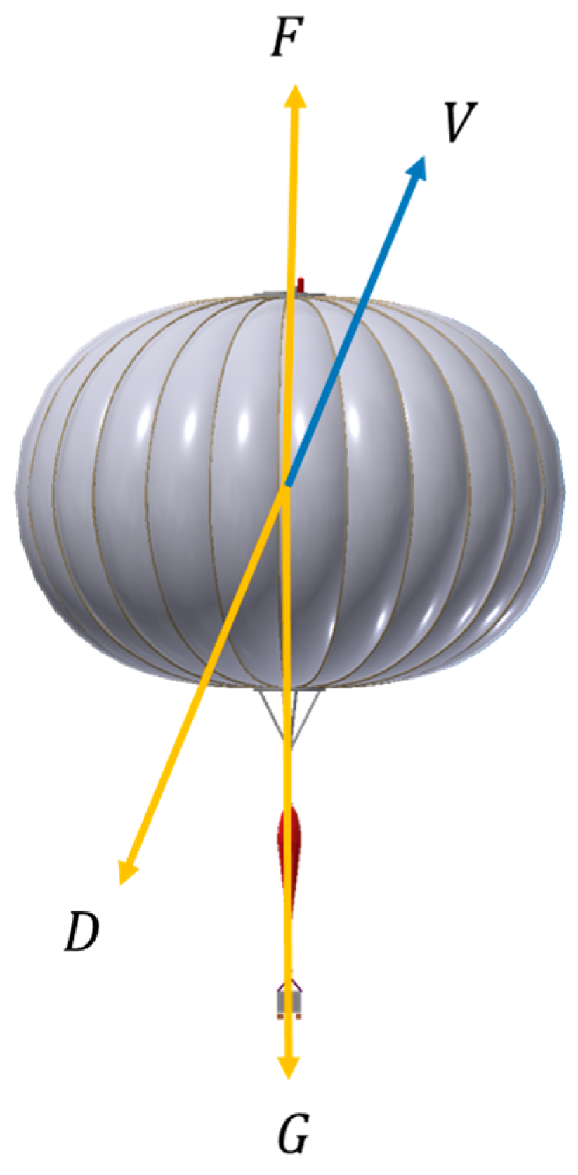
2.3.3. Dynamic Model of the Balloon

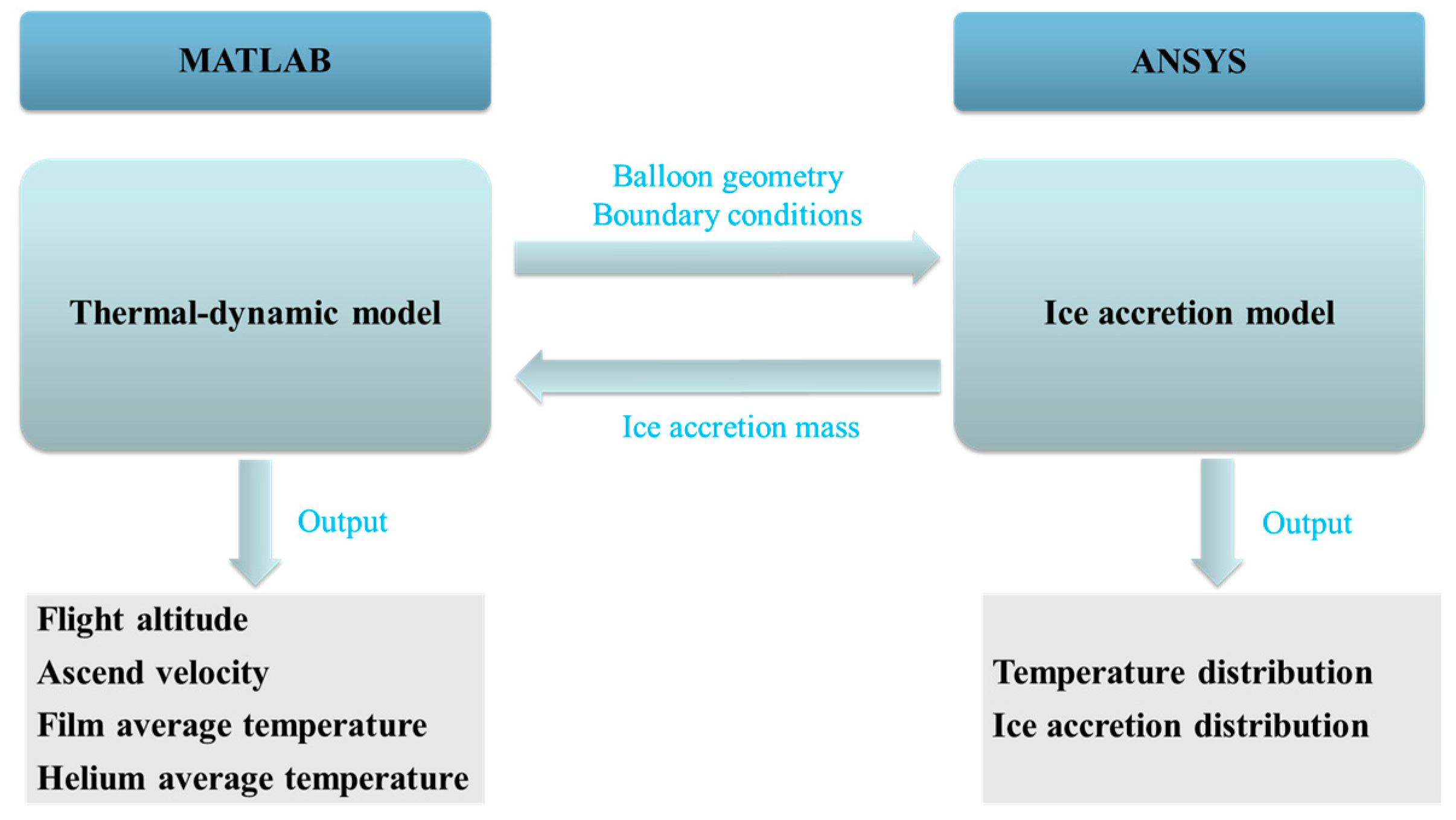
The dynamic performance of the balloon is dominated by the buoyant force ($F$), aerodynamic drag force ($D$), and gravity force ($G$); the balloon analysis mechanics are presented in a diagram in Figure 4.

The buoyant force ($F$) of the balloon is determined by Archimedes’ principle and can be calculated as follows:

$$F={\rho }_{air}·g·V$$

(38)

Here, ${\rho }_{air}$ is the air density at the balloon altitude, and $g$ represents the gravitational acceleration constant.

The aerodynamic drag force ($D$) of the balloon relates to the relative velocity ($v_r$) between the balloon and the air and the aerodynamic drag coefficient ($C_d$), and it can be calculated as follows:

$$D=-1/2{\rho }_{air}{C}_d{A}_{top}{v}_r\left|v_r\right|$$

(39)

The gravity force ($G$) of the balloon is determined by its mass and can be calculated as follows:

$$G=(m_{film}+m_{He}+m_{payload}+m_{ice})g$$

(40)

Here, $m_{film}$, $m_{He}$, $m_{payload}$, and $m_{ice}$ represent the mass of the film, helium, payload, and ice accreted on the balloon’s surface, respectively.

The dynamic differential equations of the balloon in the altitude direction can be calculated as follows:

$$M_{total}\cdot \ddot{H}=F-D-G$$

(41)

Here, $M_{total}$ is the total mass of the balloon, made up of its real mass and virtual mass, which can be calculated as follows:

$$M_{total}=m_{\mathrm{film}}+m_{\mathrm{He}}+m_{\mathrm{payload}}+m_{\mathrm{ice}}+C_{\mathrm{vir}}\cdot {\rho }_{\mathrm{air}}\cdot V$$

(42)

The virtual mass considers the mass of air dragged along with the balloon, with a virtual mass coefficient ($C_{\mathrm{vir}}$) of about 0.25 to 0.5 [4].

The relationship between the flight altitude and ascent velocity of the balloon is defined as follows:

$$\ddot{H}=d{v}_H/dt$$

(43)

3. Analysis Method

A comprehensive simulation platform was developed to simulate the influence of ice accretion on the thermodynamic performance of a scientific balloon. The simulation platform consists of two parts. One is a program developed with MATLAB to solve the thermodynamic model, while the other uses ANSYS to solve the ice accretion model. A flow chart of the simulation platform is shown in Figure 5.

When the comprehensive simulation platform runs, the MATLAB program solves the thermodynamic model and calculates the flight altitude, ascent velocity, average film temperature, and average helium temperature of the balloon and outputs the balloon geometry and boundary conditions to the ANSYS program. ANSYS discretizes the computational zone, loads boundary conditions, and solves the mass-, momentum-, and energy-governing equations in the computational zone to simulate the temperature and ice accretion distribution. Then, ANSYS outputs the ice accretion mass to MATLAB, which continues to simulate the influence of ice accretion on the balloon’s thermodynamic performance.

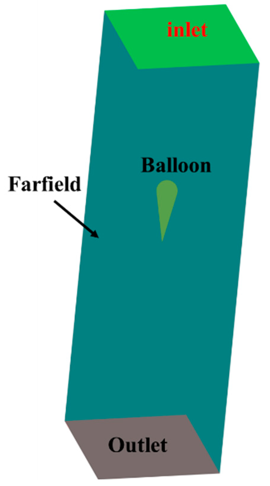
3.1. Ice Accretion Analysis Method

The ice accretion analysis program was developed with ANSYS. Sequential processing starts with ANSYS FLUENT MESHING to create a computational domain and generate mesh; then, computations are performed with ANSYS/Fluent, ANSYS/FENSAP/DROP, and ANSYS/FENSAP/ICE3D. The data flow of the ice accretion analysis is depicted in Figure 6.

The three-dimensional computational domain around the balloon is shown in Figure 7.

The inlet is the velocity inlet boundary, and the distance from the balloon is 10 times the balloon’s diameter. The four surroundings are the far-field boundary, and the distance from the balloon is 10 times the balloon’s diameter. The outlet is the pressure outlet boundary, and the distance from the balloon is 15 times the balloon’s diameter. These boundary conditions were placed far from the balloon to reduce interactions with the flow around it.

An unstructured mesh was generated to discretize the computational domain outside and inside the balloon. The mesh near the balloon’s surface was refined to achieve better simulation results. A cross-sectional mesh of the computational domain is shown in Figure 8.

A mesh sensitivity analysis was conducted with three meshes. The meshes were employed to simulate the temperature performance of the balloon in the ascending process. There were 2.834 million, 5.443 million, and 7.046 million grid cells in each mesh. The balloon temperature results for the three mesh conditions are listed in

Table 1. Mesh sensitivity analysis.

Mesh ID	No. of Grid Cells (Millions)	Surface Mean Temperature (K)	Surface Maximum Temperature (K)	Surface Minimum Temperature (K)
1	2.834	210.9	215	205
2	5.443	210.3	213	205
3	7.046	209.8	212	205

.

The data in Table 1 suggest that when the grid number increases from 2.834 million to 5.443 million, the surface mean and maximum temperature of the balloon change by about 0.6 K and 2 K, respectively. When the grid number increases from 5.443 million to 7.046 million, the surface mean and maximum temperature of the balloon change by about 0.5 K and 1 K, respectively. To ensure accuracy while improving calculation efficiency, Mesh 2 (5.443 million grid cells) was adopted for the following calculations.

3.2. Thermodynamic Analysis Method

A thermodynamic analysis program was developed with MATLAB; the structure of the program is shown schematically in Figure 9.

The program comprises four models: an atmosphere model, a balloon geometric model, a thermal model with cloud modification, and a dynamic model. When MATLAB runs, the program imports the initial data—including the balloon design index, launch time and location, and cloud properties—and solves the four models by implementing ice accretion mass data from ANSYS. Finally, it outputs the flight altitude, ascent velocity, film average temperature, and helium average temperature of the balloon under the influence of ice accretion on its surface.

4. Model Validation

4.1. Ice Accretion Model Validation

The validity and rationality of the ice accretion model employed in this study were confirmed by Concordia University in 2000 and McGill University in 2003. A detailed description of the validation can be found in [21,22].

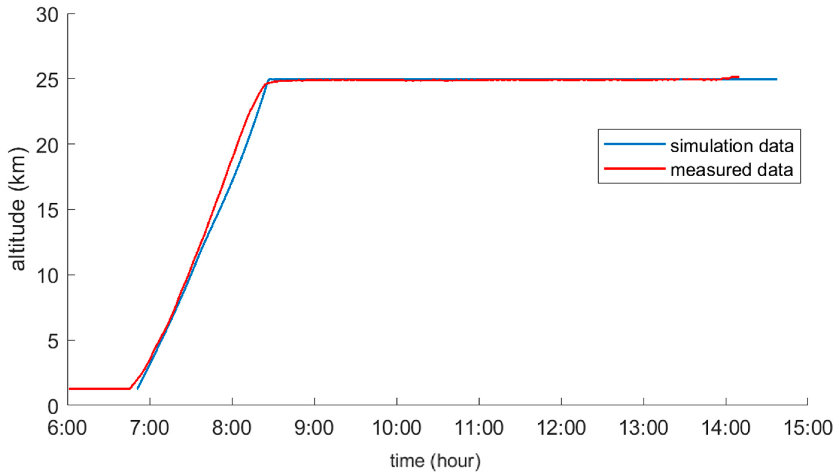
4.2. Thermodynamic Model Validation

To validate the accuracy of the thermodynamic model, we employed thermodynamic experimental data from a super-pressure balloon with a volume of 7240 cubic meters developed by the Aerospace Information Research Institute, Chinese Academy of Sciences.

The design index of the super-pressure balloon is listed in

Table 2. Design index of a super-pressure scientific balloon.

Design Index	Value
Floating altitude	25 km
Volume	7240 m3
Total mass	280 kg
Balloon film mass	120 kg
Payload mass	124 kg

.

The thermal radiation properties of the super-pressure balloon film are listed in

Table 3. Thermal radiation properties of balloon film.

$c_f(J\cdot k{g}^{-1}\cdot K^{-1})$	${\alpha }_{\mathrm{film}}$	${\tau }_{\mathrm{film}}$	${\alpha }_{\mathrm{film}-\mathrm{IR}}$	${\tau }_{\mathrm{film}-\mathrm{IR}}$
2302.7	0.02	0.9	0.078	0.9

.

Three temperature sensors were arranged along the central line inside the balloon to measure the helium temperature, as described in Figure 10.

The super-pressure balloon was launched in September 2017 in the center of the Inner Mongolia Autonomous Region, Northeast China, by the Aerospace Information Research Institute, Chinese Academy of Sciences. The launch took place at 06:45 in clear sky conditions. It took approximately 110 min for the balloon to approach its designed float altitude. The ascending and floating states of the balloon are presented in Figure 11 and Figure 12, respectively.

The flight altitude, ascent velocity, and temperature of helium are three critical parameters for representing the thermodynamic performance of a balloon. The simulation and measured data for these three parameters were compared to validate the accuracy of the thermodynamic model. The comparison is shown in Figure 13.

Figure 13 suggests that the simulation and measured data for flight altitude have the same trend and are close to each other. During the steady-float stage, the measured and simulation flight altitudes were 24.95 km and 24.9 km, respectively. There was only a tiny 0.2% discrepancy between them.

The simulation and measured data for the ascent velocity are compared in Figure 14.

Figure 14 suggests that the simulation and measured data for ascent velocity have the same trend and are close to each other. In the early stage of the launch process, the buoyancy was larger than the weight, driven by the upward net force, and the balloon ascended swiftly. The simulation and measured data velocities were 3.5 m/s and 2.5 m/s, respectively. In the ascending stage, influenced by environment temperature changes and helium expansion, the ascent velocity simulation data changed in a W shape, and the measured data changed more randomly. The maximum simulation and measured data for the ascent velocity were 5.7 m/s and 5.5 m/s, with a discrepancy of 3.5% between them. The average simulation and measured data for ascent velocity were 2.4 m/s and 2.8 m/s, with a discrepancy of 14.3% between them. During the floating stage, when the balloon approached its designed float altitude, the ascent velocity swiftly decreased to 0 m/s and oscillated around 0 m/s; this phenomenon is represented by both the simulation and measured data.

The simulation and measured data for the helium temperature are compared in Figure 15.

Figure 15 suggests that the simulation and measured data for the helium temperature have the same trend and are close to each other. The initial temperature of the helium was about 280 K. In the early stage of the launch process, the balloon expanded, its volume swiftly increased, and the environmental temperature rapidly decreased; this enhanced the internal convection heat transfer between the balloon film and the helium and the external convection heat transfer between the balloon film and the environment. Owing to work performed on the outside of the balloon, the temperature of the helium decreased quickly. The minimum simulation and measured data for the helium temperature were 212 K and 209.3 K, with a discrepancy of 2.7 K. During the floating stage, the balloon volume no longer expanded, and the solar radiation intensity influenced the helium temperature. The maximum simulation and measured data for the helium temperature were 260.5 K and 258.5 K, with a discrepancy of 2 K.

The comparisons between the simulation and measured data for flight altitude, ascent velocity, and helium temperature demonstrated that the thermodynamic model developed in this study is highly accurate. It can simulate the thermodynamic performance of a balloon in a clear sky environment, laying a solid foundation for further investigations into the influence of ice accretion on balloon surfaces.

5. Results and Discussion

Ice accretion and its influence on the thermodynamic performance of a scientific balloon were investigated. The balloon in this investigation was a 7240-cubic-meter balloon launched in September 2017. The cloud parameters were obtained from the Chinese FY-4 satellite [23]; the altitudes of the cloud top and base were 13.7 km and 12.5 km, respectively; and the cloud temperature was 205 K.

5.1. Ice Accretion Performance

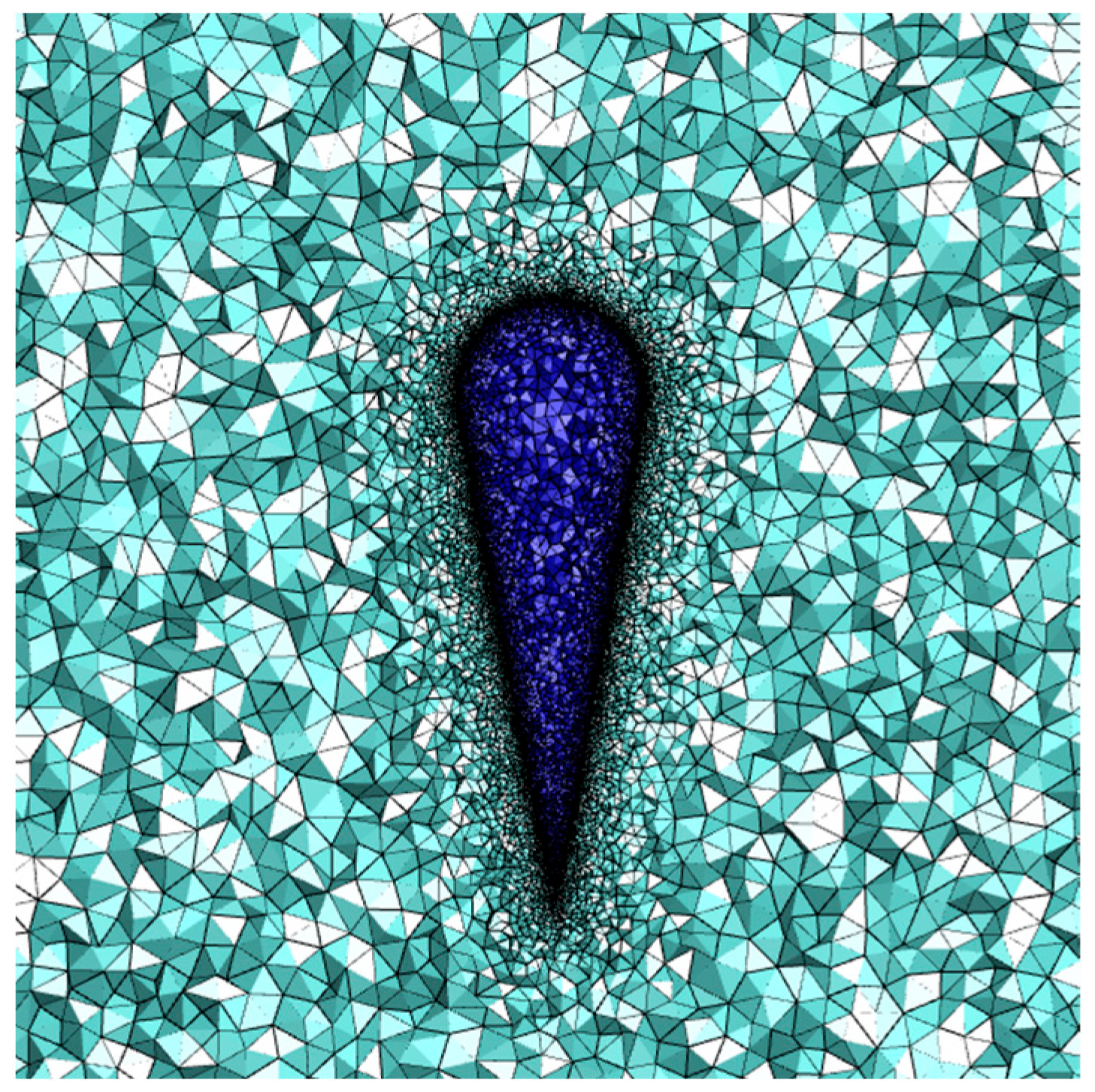
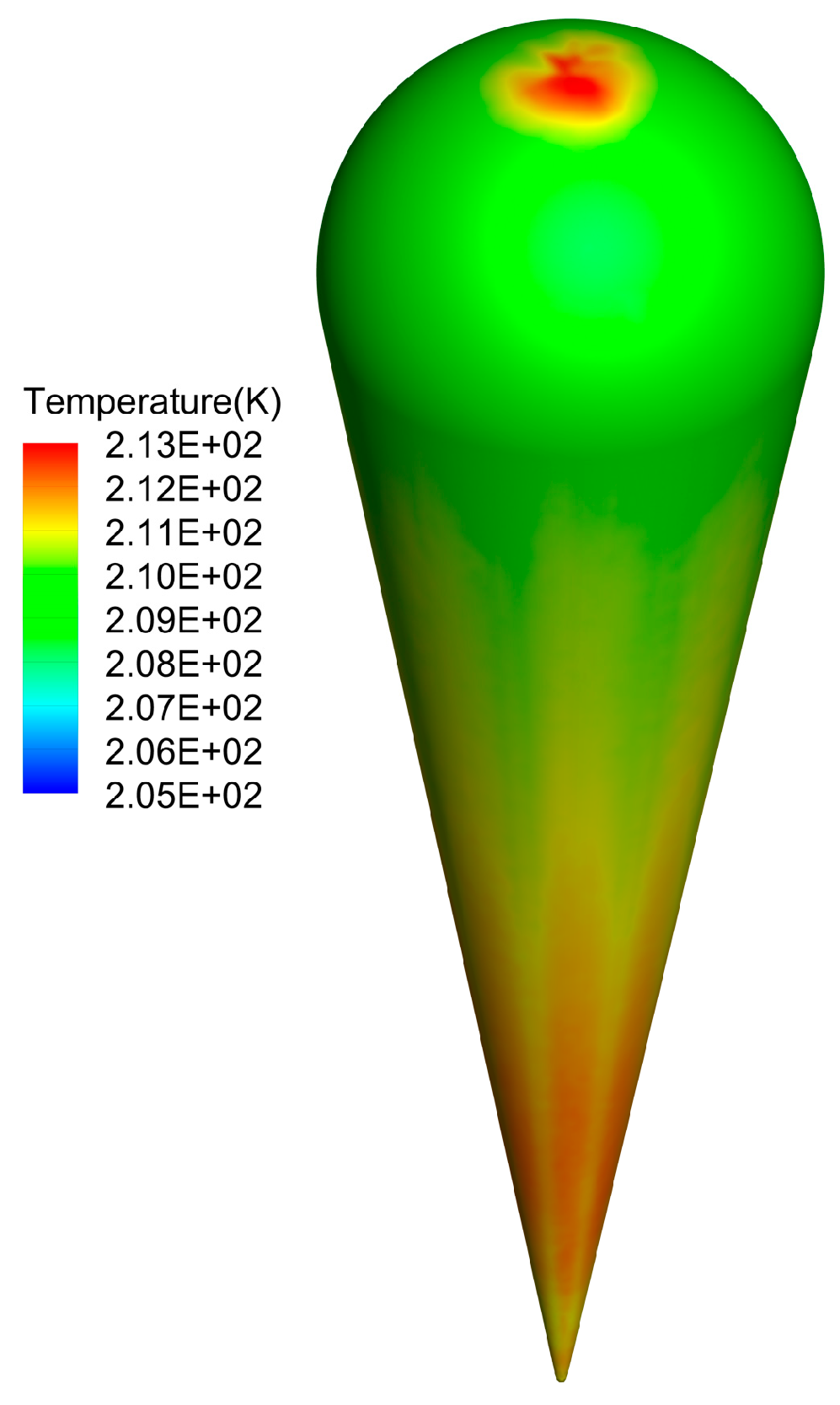
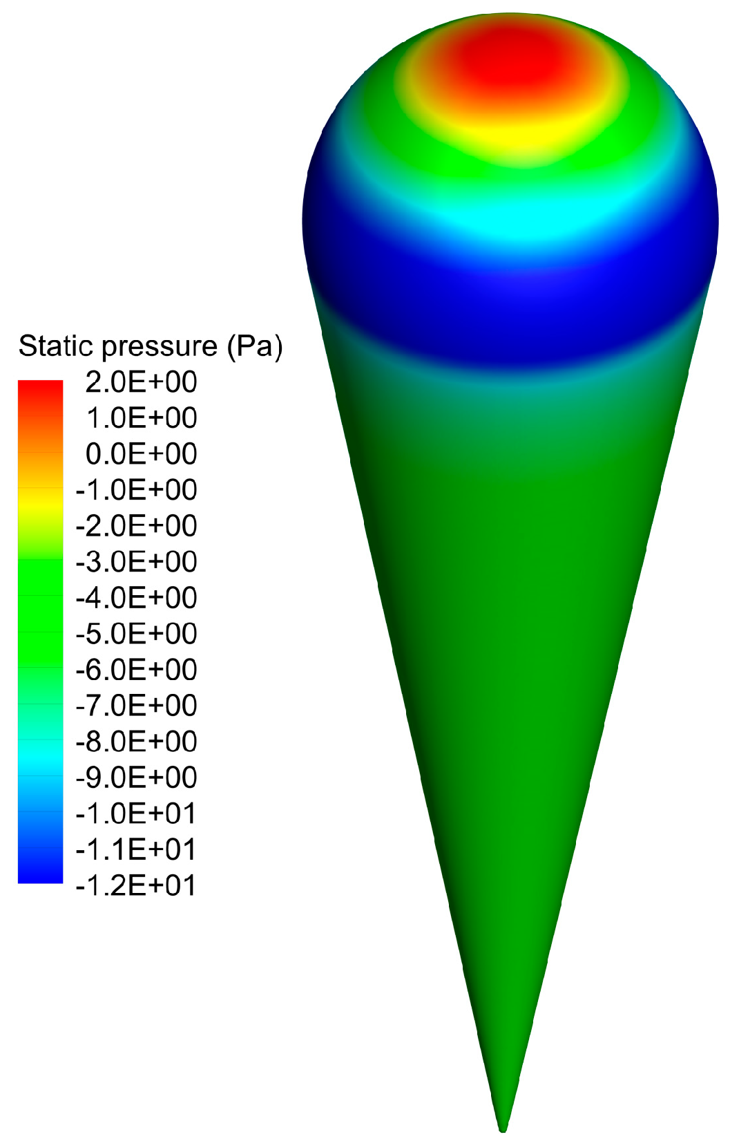
5.1.1. Temperature and Flow Distribution

The thermal and flow fields of the balloon when rising through clouds are analyzed in this section to determine if there is a chance of ice accretion on the balloon’s surface while the balloon ascends with a velocity of 3 m/s and an atmosphere temperature of 205 K.

The temperature distribution of the balloon’s surface is described in Figure 16.

Figure 16 suggests that higher temperatures were located on the upper and lower parts of the balloon, while lower temperatures were distributed on the side of the balloon. The maximum temperature was about 213 K, and the difference was about 6 K. The balloon’s surface temperature was lower than the icing point of 273.15 K, so ice accretion on the surface is possible when rising through icy clouds.

The airflow field of the balloon was investigated to provide input data to calculate droplet impingement and ice accretion on the balloon surface. The pressure distribution on the balloon surface is presented in Figure 17.

Figure 17 shows that higher pressure was distributed on the windward surface of the balloon, such as the upper part, while lower pressure was distributed on the side. The maximum static pressure was 2 Pa higher than the local atmosphere, and the minimum static pressure was 12 Pa lower than the local atmosphere. Additionally, the pressure distribution on the lower part of the balloon was relatively uniform.

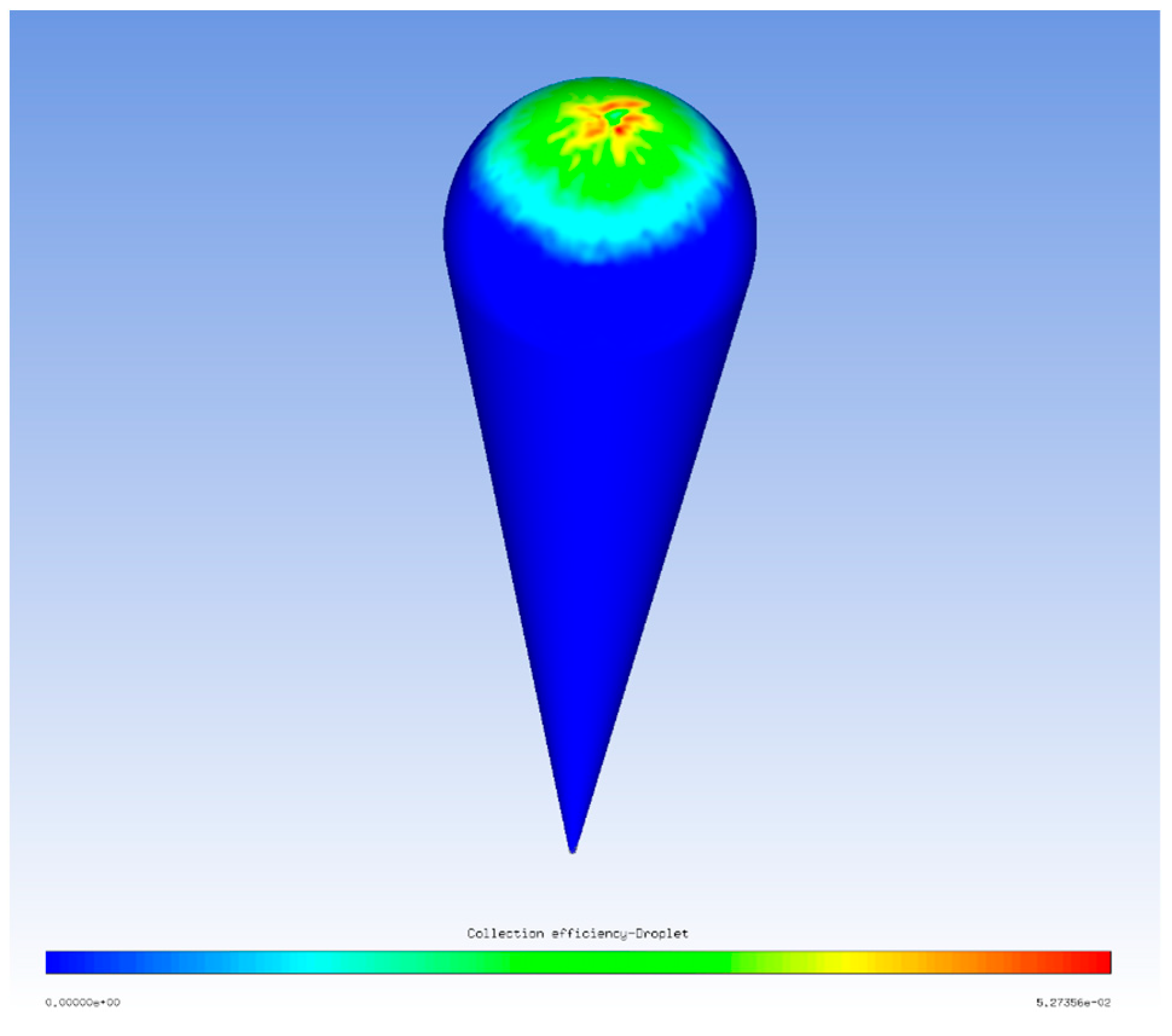
5.1.2. Droplet Collection Efficiency Distribution

The temperature and flow field results suggest that, when the balloon rises through an icy cloud, its surface temperature is below 273.15 K. A risk of ice accretion on the balloon surface may be present under these conditions, so the droplet impingement performance was investigated for these circumstances.

The mesh and airflow results calculated using FLUENT were imported into the FENSAP-DROP3D module to calculate droplet impingement performance. The environmental temperature was 205 K, the median diameter of the droplets was 50 μm, the liquid water content of the droplets was $5\times {10}^{-3} \mathrm{kg}/{\mathrm{m}}^3$, and the ascent velocity was 3 m/s.

The droplet collection efficiency distribution on the balloon surface is represented in Figure 18.

The droplet collection efficiency distribution agreed with the pressure distribution. The maximum droplet collection efficiency area was located on the top point of the upper part of the balloon and was about 0.0527.

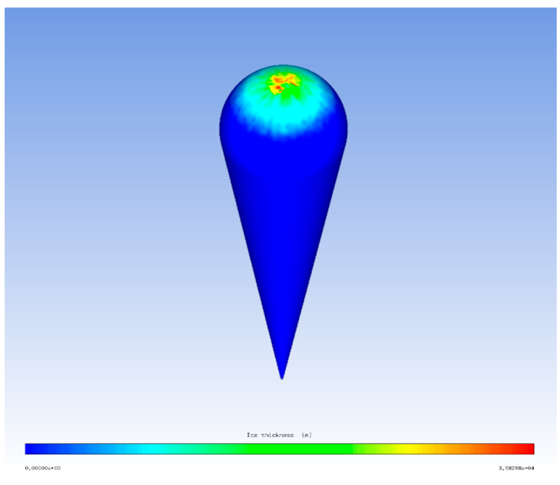
5.1.3. Ice Accretion Distribution

The mesh and droplet collection efficiency results were imported into the FENSAP-ICE3D module to calculate ice accretion performance on the balloon’s surface.

The environment temperature was 205 K, the median diameter of the droplets was 50 μm, the liquid water content of the droplets was $5\times {10}^{-3} \mathrm{kg}/{\mathrm{m}}^3$, and the ascent velocity was 3 m/s. A total ice accretion time of 420 s was simulated with a time step of 0.001 s.

The ice accretion distribution on the balloon’s surface and the total mass of ice accretion are described in Figure 19 and Figure 20, respectively.

Figure 19 suggests that the ice accretion distribution agreed with the droplet collection efficiency distribution. Thicker ice was distributed on the windward part of the balloon surface, and thinner ice was distributed on the rest of the balloon. After 420 s of accretion, the maximum ice thickness was about 0.000358 m.

Figure 20 suggests that after 420 s of accretion, the total ice accretion mass was 59.5 kg. The mass rate of ice accretion was about 0.14 kg/s.

5.2. Influence of Ice Accretion

In this section, the influence of ice accretion on the flight altitude, ascent velocity, helium temperature, and helium super pressure are investigated in detail.

When the balloon ascended through an icy cloud, the super-cooled droplets in the cloud impinged the balloon and accreted ice on its surface. The altitudes of the cloud top and base were 13.7 km and 12.5 km, respectively, and the cloud temperature was 205 K.

The ice accretion mass rate was 0.14 kg/s when the balloon entered the cloud, and the ice melt mass rate was assumed to be 0.14 kg/s when the balloon dropped out of the cloud.

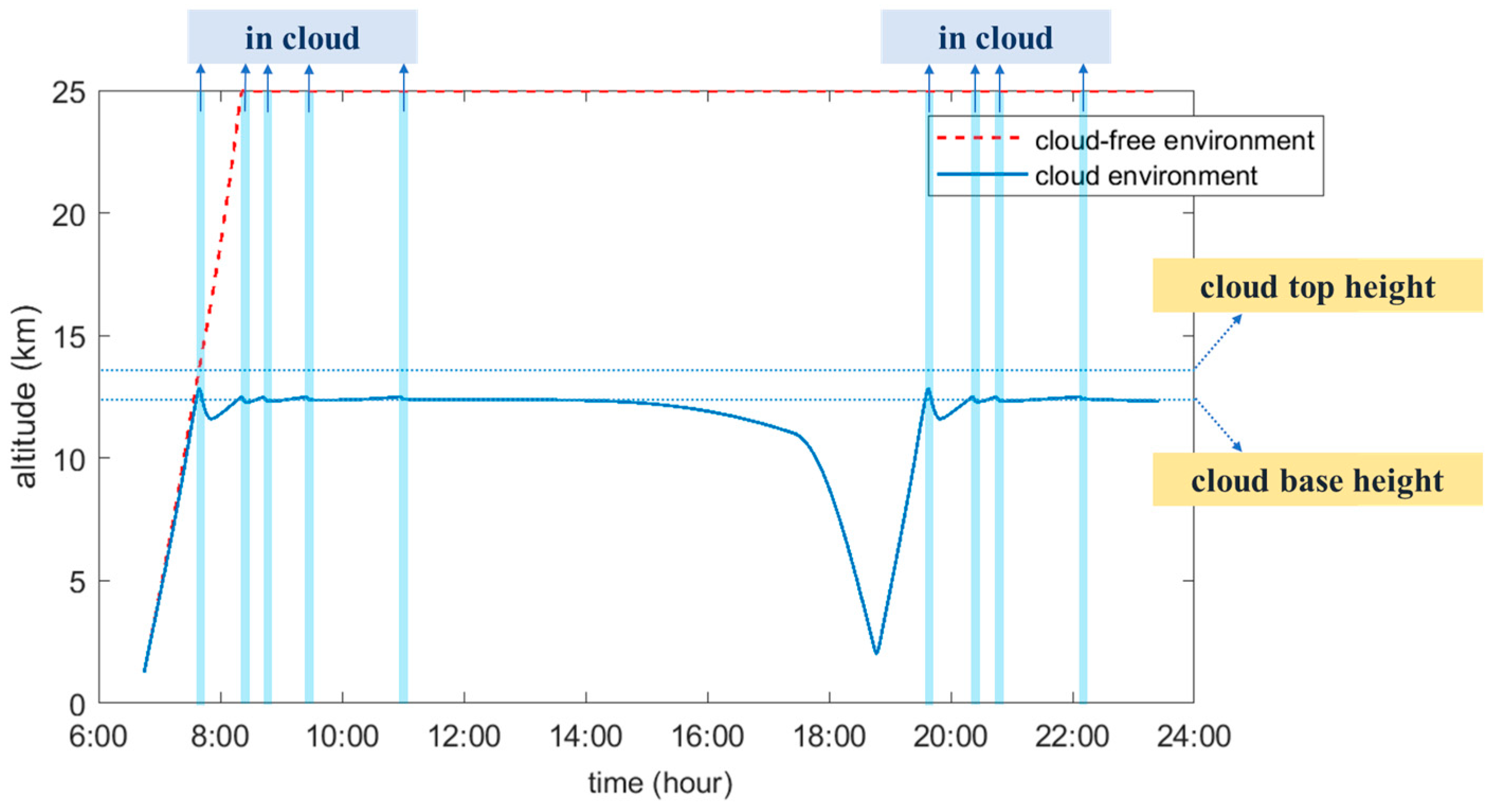
5.2.1. Flight Altitude

The flight altitude data for the balloon under the influence of ice accretion according to the model are shown in Figure 21. The red dashed line represents the flight altitude data for clear skies, and the blue line represents the flight altitude data for a cloud environment.

Figure 21 shows that, in the cloud-free environment, the balloon ascended swiftly after launch and finally floated at an altitude of about 25 km. However, in the cloud environment, under the influence of ice accretion, the balloon could not ascend; it floated at the base of the clouds.

The balloon was launched at about 6:45 and entered the clouds at about 7:36. Then, it floated at the base of the clouds until about 16:00; from 16:00 to 20:00, it experienced another flight altitude change and finally floated at the base of the clouds.

These phenomena occurred because when the balloon ascended and entered the clouds at about 7:36, ice accreted on its surface. The upward buoyance force was larger than the downward gravity force in the early stage of this process, and the balloon continued to ascend until the ice accumulated enough to balance its upward buoyance, ending its ascent. The ice accreted on the balloon’s surface in the clouds, and when it reached its maximum height in the clouds, it started to descend. Once the balloon descended from the clouds, the ice accreted on its surface began to melt, and it started to ascend again. Dominated by ice accretion and the melting process, the flight height of the balloon oscillated near the cloud base.

The first time the balloon ascended, it rose about 0.5 km into the cloud and then dropped by about 1.1 km. It then floated near the base. At 16:00, the solar radiation intensity decreased, and the balloon dropped its flight altitude. At 18:50, the balloon flight altitude reached its lowest point, 0.73 km above the Earth’s surface. The environmental temperature was well above the icing point, and the ice accreted on the balloon surface began to melt; thus, the balloon ascended once again to the cloud base.

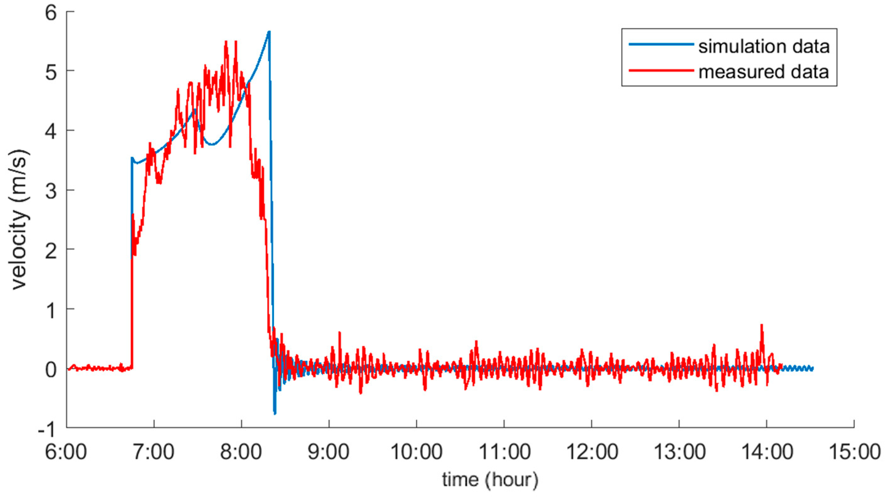
5.2.2. Ascent Velocity

The ascent velocity data for the balloon under the influence of ice accretion are described in Figure 22. The red dashed line represents the ascent velocity data for clear skies, and the blue line represents the ascent velocity data for a cloud environment.

Figure 22 suggests that in the cloud-free environment, the ascent velocity changed in a W shape during the ascent stage, oscillating around 0 m/s during the float stage. However, when the balloon entered the cloud environment at 7:36, and ice accreted on its surface, the ascent velocity dramatically decreased from about 3.8 m/s to −3.1 m/s. At 18:50, the balloon experienced another dramatic ascent velocity change. Dominated by ice accretion and the melting process, each time the balloon entered the clouds, it fell, with the ascent velocity oscillating near zero.

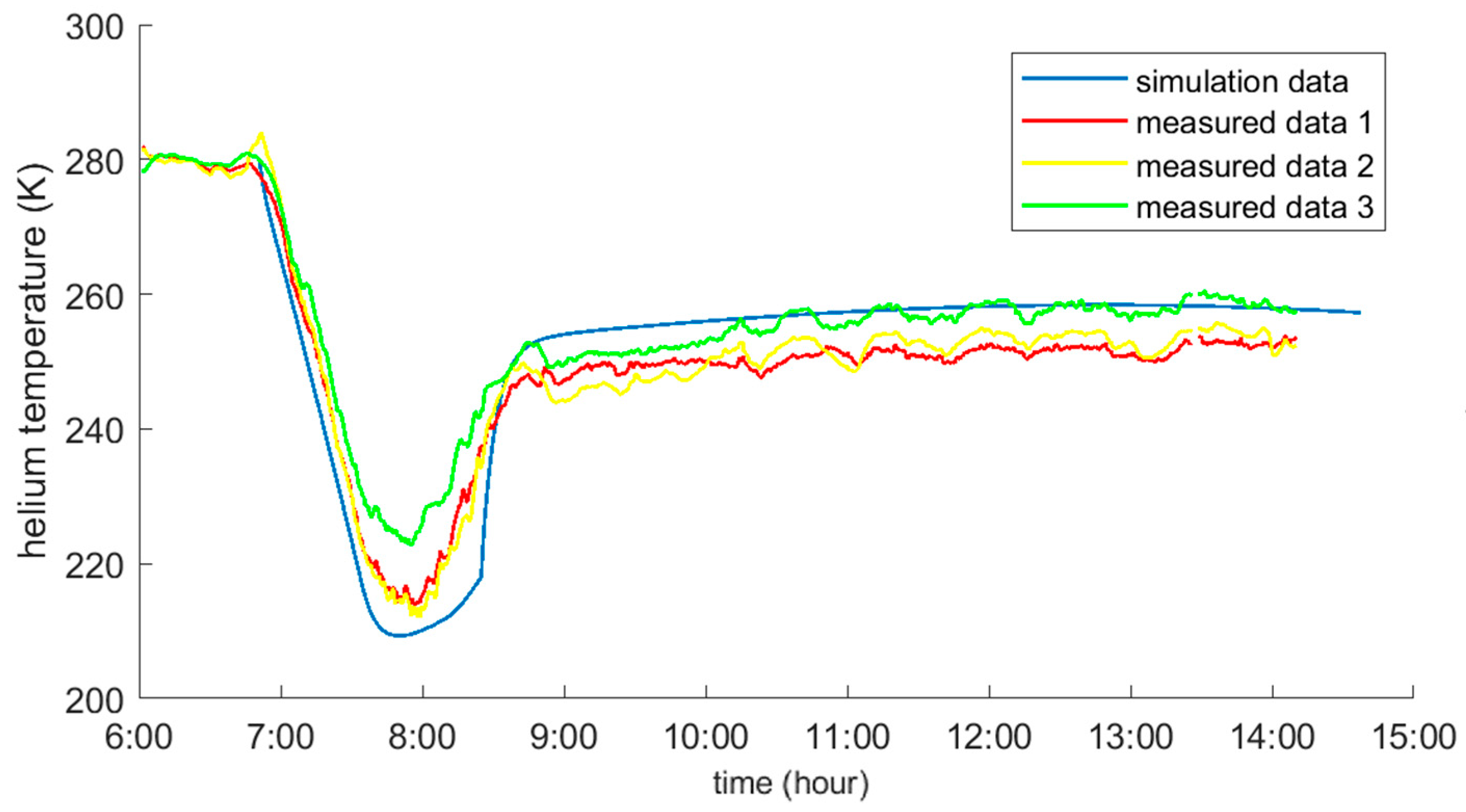
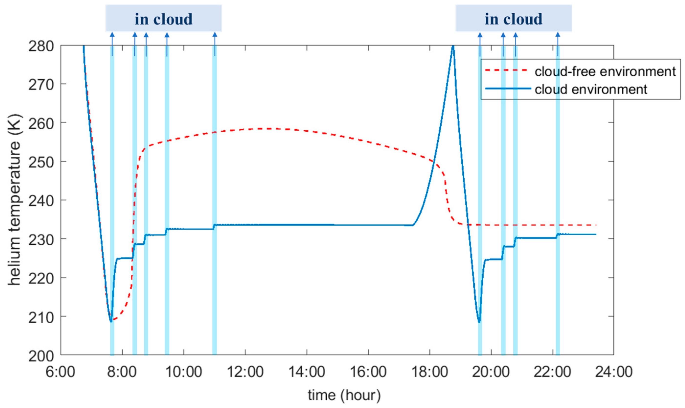
5.2.3. Helium Temperature

The helium temperature data for the balloon under the influence of ice accretion are described in Figure 23. The red dashed line represents the helium temperature data for clear skies, and the blue line represents the helium temperature data for a cloud environment.

Figure 23 suggests that in the cloud-free environment, the helium temperature quickly decreased to about 212 K during the ascent stage. The helium temperature quickly increased and reached about 260.5 K at midday during the float stage. However, in the cloud environment, under the influence of ice accretion, volume expansion during the ascent from 6:45 to 7:36 swiftly decreased the helium temperature from 280 K to 210 K. When the balloon floated near the base of the cloud from 07:50 to 17:20, the helium temperature was dominated by the cloud temperature and influenced by solar radiation, increasing slowly from 225 K to 232 K. From 17:20 to 18:50, the helium swiftly temperature increased from 232 K to 280 K; this was because the balloon’s flight altitude dropped to its lowest point, and the environmental temperature swiftly increased. From 20:00 to 23:30, the helium temperature increased and finally reached close to 231 K.

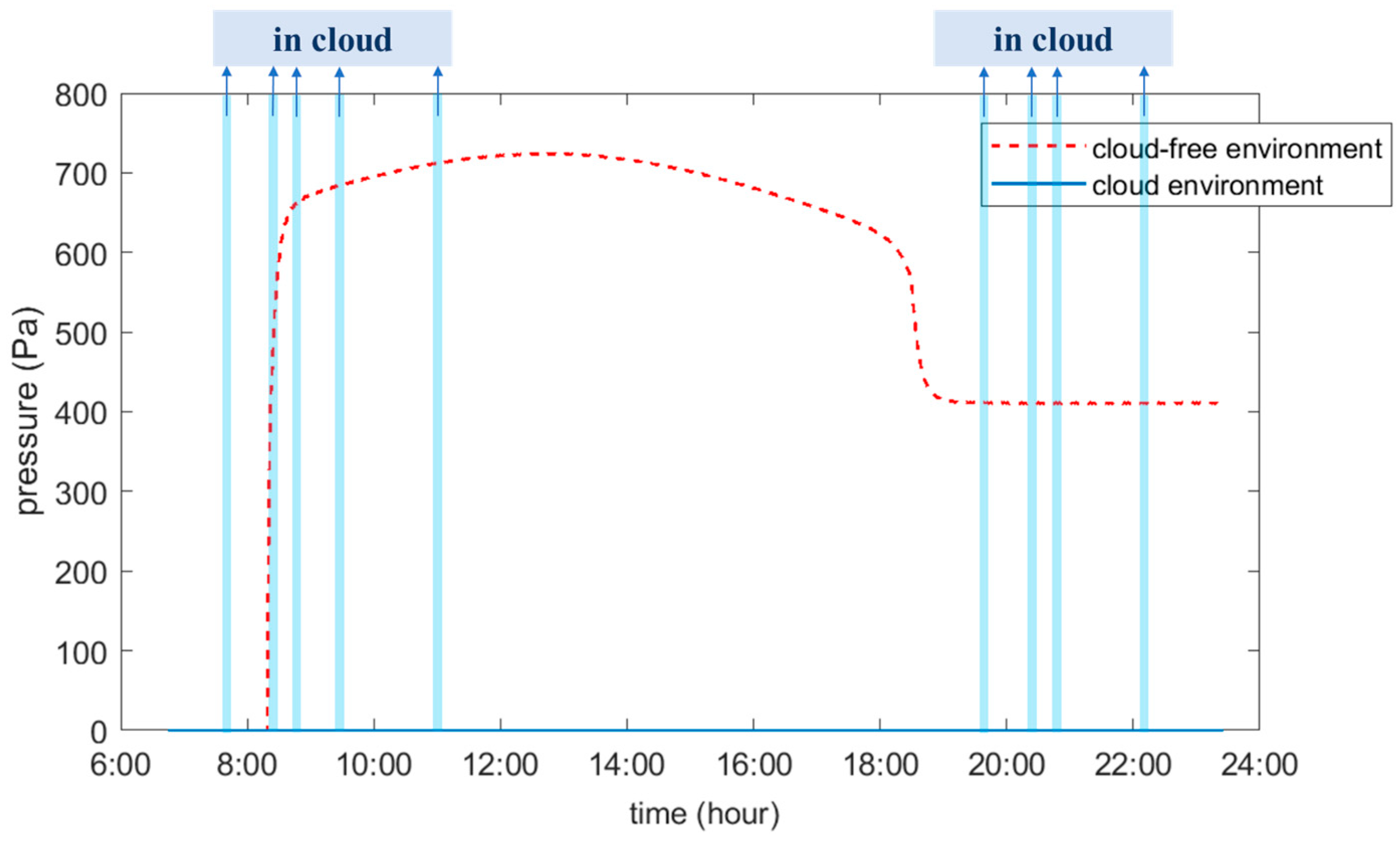
5.2.4. Helium Super Pressure

The helium super-pressure data for the balloon under the influence of ice accretion are described in Figure 24. The red dashed line represents the helium super-pressure data for clear skies, and the blue line represents the helium super-pressure data for a cloud environment.

Figure 24 suggests that, in the cloud-free environment, the helium super pressure quickly increased and reached about 715 Pa at midday during the float stage. However, in the cloud environment, under the influence of ice accretion, the helium super pressure remained at zero because the balloon could not ascend above the clouds and was not fully inflated.

6. Conclusions

A comprehensive simulation platform with cloud modification was proposed herein to simulate the influence of ice accretion on the thermodynamic performance of a scientific balloon. The ice accretion performance of the scientific balloon in an icy cloud environment was numerically analyzed, and a further investigation into the influence of ice accretion was conducted. We can draw the following conclusion from the results:

(1)

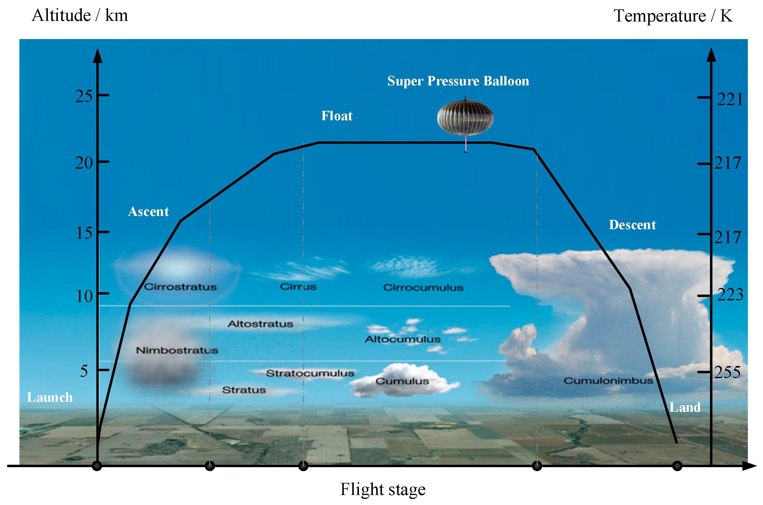
When a scientific balloon ascends through clouds, the clouds influence its thermal environment. When the balloon’s surface temperature is below the icing point of 273.15 K, and it encounters ice droplets in clouds, there is a risk of ice accretion on the surface;

(2)

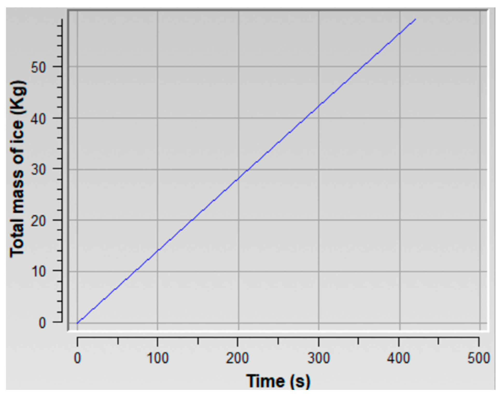
In an icing situation, thicker ice is distributed on the windward part of the balloon’s surface, and thinner ice is distributed on the rest of the balloon. Under certain conditions, the maximum ice thickness can be 0.000358 m after 420 s of ice accretion. In this study, the total ice accretion mass was 59.5 kg, and the mass rate of ice accretion was about 0.14 kg/s;

(3)

Ice accretion on the balloon’s surface influences its thermodynamic performance. When the mass rate of ice accretion is about 0.14 kg/s, ice accretion prevents the balloon from ascending through the clouds and causes it to remain floating at the base of the clouds.

References

1. Colozza, A. High-Altitude, Long-Endurance Balloons for Coastal Surveillance; NASA TM-2005-213427; NASA: Washington, DC, USA, 2005. [Google Scholar]
2. Kreith, F.; Kreider, J.F. Numerical Prediction of the Performance of High Altitude Balloons; NCAR Technical Note NCAR-IN/STR-65; Atmospheric Technology Division, National Center for Atmospheric Research: Boulder, CO, USA, 1974. [Google Scholar]
3. Carlson, L.A.; Horn, W.J. A New Thermal and Trajectory Model for High Altitude Balloons. In Proceedings of the 7th AIAA Aerodynamic Decelerator and Balloon Technology Conference, San Diego, CA, USA, 21–23 October 1981. [Google Scholar]
4. Farley, R.E. BalloonAscent: 3-D simulation tool for the ascent and float of High-Altitude Balloons. In Proceedings of the AIAA 5th Aviation, Technology, Integration, and Operations Conference, AIAA 2005-7412, Arlington, VA, USA, 26–28 September 2005. [Google Scholar]
5. Dai, Q.M.; Fang, X.D.; Li, X.; Tian, L. Performance simulation of high altitude scientific balloons. Adv. Space Res. 2012, 49, 1045–1052. [Google Scholar] [CrossRef]
6. Louchev, O.A. Steady state model for the thermal regimes of shells of airships and hot air balloons. Int. Heat Mass Transf. 1992, 35, 2683–2693. [Google Scholar] [CrossRef]
7. Xia, X.L.; Li, D.F.; Sun, C.; Ruan, L.-M. Transient behavior of stratospheric balloons at float conditions. Adv. Space Res. 2010, 46, 1184–1190. [Google Scholar] [CrossRef]
8. Wang, Y.W.; Yang, C.X. A comprehensive numerical model examining the thermal performance of airships. Adv. Space Res. 2011, 48, 1515–1522. [Google Scholar] [CrossRef]
9. Liu, Q.; Wu, Z.; Zhu, M.; Xu, W. A comprehensive numerical model investigating the thermal-dynamic performance of scientific balloon. Adv. Space Res. 2014, 53, 325–338. [Google Scholar] [CrossRef]
10. Messinger, B.L. Equilibrium temperature of an unheated icing surface as a function of air speed. Aeronaut. Sci. 1953, 20, 29–42. [Google Scholar] [CrossRef]
11. Shen, X.B.; Lin, G.P.; Yu, J.; Bu, X.Q.; Du, C.H. Three-Dimensional Numerical Simulation of Ice Accretion at the Engine Inlet. J. Aircraft. 2013, 50, 635–642. [Google Scholar] [CrossRef]
12. Cao, Y.; Huang, J.; Yin, J. Numerical simulation of three-dimensional ice accretion on an aircraft wing. Int. J. Heat Mass Transf. 2016, 92, 34–54. [Google Scholar] [CrossRef]
13. Liu, Q.; Yang, Y.; Wang, Q.; Cui, Y.; Cai, J. Icing performance of stratospheric airship in ascending process. Adv. Space Res. 2019, 64, 2405–2416. [Google Scholar] [CrossRef]
14. Muhammed, M.; Virk, M.S. Ice Accretion on Fixed-Wing Unmanned Aerial Vehicle—A Review Study. Drones 2022, 6, 86. [Google Scholar] [CrossRef]
15. Muhammed, M.; Virk, M.S. Ice Accretion on Rotary-Wing Unmanned Aerial Vehicles—A Review Study. Aerospace 2023, 10, 261. [Google Scholar] [CrossRef]
16. Slingo, A. A GCM parameterization for the shortwave radiative properties of water clouds. J. Atmos. Sci. 1989, 46, 1419–1427. [Google Scholar] [CrossRef]
17. Lindner, T.H.; Li, J. Parameterization of the optical properties for water clouds in the infrared. J. Clim. 2000, 13, 1797–1805. [Google Scholar] [CrossRef]
18. Stephens, G.L.; Ackerman, S.; Smith, E.A. A shortwave parameterization revised to improve cloud absorption. J. Atmos. Sci. 1984, 41, 687–690. [Google Scholar] [CrossRef]
19. Sun, Z.; Liu, J.; Zeng, X.N.; Liang, H. Estimation of global and net solar radiation at the Earth surface under cloudy-sky condition. J. Meteorol. Environ. 2014, 30, 1–9. [Google Scholar]
20. Chylek, P.; Ramaswamy, V. Simple approximation for infrared emissivity of water clouds. J. Atmos. Sci. 1982, 39, 171–177. [Google Scholar] [CrossRef]
21. Bourgault, Y.; Boutanios, Z.; Habashi, W.G. Three-Dimensional Eulerian Approach to Droplet Impingement Simulation Using FENSAP-ICE Part 1 Model, Algorithm, and Validation. J. Aircr. 2000, 37, 95–103. [Google Scholar] [CrossRef]
22. Beaugendre, H.; Morency, F.; Habashi, W.G. FENSAP-ICEs Three-Dimensional In-Flight Ice Accretion Module ICE3D. J. Aircr. 2003, 40, 239–247. [Google Scholar] [CrossRef]
23. Satellite Weather Application Platform v2.0. Available online: http://rsapp.nsmc.org.cn/geofy (accessed on 28 May 2023).
Figure 1. Cloud environment around a scientific balloon.
Aerospace 11 00899 g001
Figure 2. Relationship between the three ice accretion modules.
Aerospace 11 00899 g002
Figure 3. Thermal environment of a scientific balloon in a cloud.
Aerospace 11 00899 g003
Figure 4. Mechanical analysis of balloon pressure.
Aerospace 11 00899 g004
Figure 5. Flow chart of the simulation platform.
Aerospace 11 00899 g005
Figure 6. Data flow of the ice accretion analysis.
Aerospace 11 00899 g006
Figure 7. Three-dimensional computational domain and boundary conditions of a scientific balloon.
Aerospace 11 00899 g007
Figure 8. Cross-sectional mesh of computational domain.
Aerospace 11 00899 g008
Figure 9. Structure of the thermodynamic simulation program.
Aerospace 11 00899 g009
Figure 10. Distribution of temperature sensors inside the balloon.
Aerospace 11 00899 g010
Figure 11. Ascending state of the balloon.
Aerospace 11 00899 g011
Figure 12. Floating state of the balloon.
Aerospace 11 00899 g012
Figure 13. Flight altitude data comparison.
Aerospace 11 00899 g013
Figure 14. Ascent velocity data comparison.
Aerospace 11 00899 g014
Figure 15. Helium temperature data comparison.
Aerospace 11 00899 g015
Figure 16. Temperature distribution of balloon surface.
Aerospace 11 00899 g016
Figure 17. Static pressure distribution on the balloon’s surface.
Aerospace 11 00899 g017
Figure 18. Droplet collection efficiency distribution on the balloon’s surface.
Aerospace 11 00899 g018
Figure 19. Ice accretion distribution on the balloon’s surface.
Aerospace 11 00899 g019
Figure 20. Total ice accretion mass.
Aerospace 11 00899 g020
Figure 21. Flight altitude performance with the influence of ice accretion.
Aerospace 11 00899 g021
Figure 22. Ascent velocity performance under the influence of ice accretion.
Aerospace 11 00899 g022
Figure 23. Helium temperature performance under the influence of ice accretion.
Aerospace 11 00899 g023
Figure 24. Helium pressure performance under the influence of ice accretion.
Aerospace 11 00899 g024