Flexible Natural Language-Based Image Data Downlink Prioritization for Nanosatellites

Abstract

Nanosatellites increasingly produce more data than can be downlinked within a reasonable time due to their limited bandwidth and power. Therefore, an on-board system is required to prioritize scientifically significant data for downlinking, as described by scientists. This paper determines whether natural language processing can be used to prioritize remote sensing images on CubeSats with more flexibility compared to existing methods. Two approaches implementing the same conceptual prioritization pipeline are compared. The first uses YOLOv8 and Llama2 to extract image features and compare them with text descriptions via cosine similarity. The second approach employs CLIP, fine-tuned on remote sensing data, to achieve the same. Both approaches are evaluated on real nanosatellite hardware, the VERTECS Camera Control Board. The CLIP approach, particularly the ResNet50-based model, shows the best performance in prioritizing and sequencing remote sensing images. This paper demonstrates that on-orbit prioritization using natural language descriptions is viable and allows for more flexibility than existing methods.

1. Introduction

Nanosatellites have become a valuable enabler for a variety of on-orbit experiments and research. A number of organizations and universities have worked to develop the CubeSat, a class of nanosatellite, around the concept of providing small, low-construction-cost, low-launch-cost space experiment platforms [1]. The complexity of CubeSat missions have increased over time thanks to improvements to and miniaturization of enabling technologies and mission payloads. This has resulted in a dramatic increase in the quantity of data produced by nanosatellites in orbit.

For example, nanosatellites such as Kyushu Institute of Technology’s own VERTECS 6U astronomical nanosatellite [2], and other CubeSats like it [3,4,5], will generate large volumes of data thanks to the inclusion of modern high-resolution imaging sensors. The small form-factor imposed by the CubeSat standard often results in major limitations and constraints on the on-board computing, power generation, and data downlink capabilities of nanosatellites [6]. The constraint on data downlink capability is of particular concern as this would limit the rate at which data can be retrieved from a CubeSat, delaying full mission success and impeding the generation of scientific value. This is an issue seen in nanosatellites of various sizes and form factors, particularly in those built to conform to the smallest form factors where the constraints placed on power, computing, and communication are most severe. Efficient on-board data processing and high-speed data downlink are required to ensure the successful completion of these missions within the required time frame.

Despite the constraints and difficulties inherent to the CubeSat platform, thanks to performance improvements and miniaturization of computing hardware, the inclusion of capable general-purpose computing platforms has seen an increase in nanosatellites. To list a few examples, BIRDS-5 included a Raspberry Pi Zero [6], KITSUNE included a Raspberry Pi Compute Module 3+ [7], BroncoSat-1 included an Nvidia Jetson Nano [8], and VERTECS will include a Raspberry Pi Compute Module 4 [9]. The inclusion of such hardware in nanosatellites, along with the constraints on data downlink rate and bandwidth, has encouraged a shift in the data processing paradigm used on CubeSats to that of orbital edge computing (OEC), where some or all data processing is carried out on the satellite in orbit, filtering and reducing the quantity of data that need to be downlinked [10,11]. OEC is presented as an alternative to the bent-pipe architecture of traditional satellite systems and is enabled by collocating processing hardware with sensors in small, low-cost satellites [10]. This would enable the use of on-board artificial intelligence (AI) and data processing algorithms for reducing the quantity of data required for downlink, as well as for facilitating the automated control of satellites and data acquisition.

However, to make use of the improved hardware, new data processing methods and novel algorithmic pipelines are required which can accurately process and filter the data commonly generated on CubeSats, such as remote sensing (RS) images and space weather measurements. Any method or algorithm considered should also run efficiently on the target hardware, while being simple and intuitive to use so that the desired data are returned to the ground easily. Modern machine learning (ML) and natural language processing (NLP) have revolutionized the way in which data are processed and computers are interacted with. It is believed that the state-of-the-art (SOTA) methods from these domains can be scaled and implemented to enable OEC and reduce the constraint on data downlink by maximizing the scientific value of downlinked data. In other words, these methods can be used to filter, select, and prioritize the most desired data for downlink first.

Some recent work has considered the problem of on-board prioritization of nanosatellite data for downlink. Chatar et al., 2023 [12] considered the downlink prioritization of astronomical images based on the classifications that are assigned on-board a 6U CubeSat. The approach used the CubeSatNet convolutional neural network (CNN) [13] to classify images into five classes, four of which indicated some sort of error and one indicating that the image should be prioritized for downlink. Classification was performed on a Raspberry Pi Compute Module 4 with classification taking about 0.29 s per image. Chatar et al., 2024 [6] explored a more robust type of satellite image prioritization, this time for RS images. The approach used the result of on-board image segmentation to prioritize images with clear captures of water bodies and vegetated areas. A UNet-based [14] segmentation algorithm segmented RS images based on five classes. Each class was given an appropriate weighting, linked to class desirability, by scientists and satellite operators so that a priority index could be calculated for an image based on the coverage estimate for each class. The prioritization pipeline was tested and validated on both the Raspberry Pi Zero and Raspberry Pi 4, as hardware targets indicative of real CubeSat hardware.

While these existing methods offer promising results, they provide poor flexibility as they are limited to the few classes which they are trained on. They also cannot consider cases which do not fall cleanly within a single class or that involve more complex interactions between two or more classes. NLP has the potential to offer increased flexibility, as the concepts which can be expressed through natural language allow for more granularity compared to using distinct classifications alone.

Qiu et al. [15] introduced Science Captioning of Terrain Images (SCOTI) for on-board data downlink prioritization for planetary rovers. Data bandwidth is very limited between planetary rovers and ground-based data systems. The authors presented a system which made use of image captioning and visual attention mechanisms to allow planetary rovers to have a sort of understanding of the images they capture. The text similarity between the captions generated by the rover and the text input by scientists were used to prioritize images for downlink based on how scientifically useful they may be. This prioritization system was designed to run entirely on the planetary rover. While planetary rovers also feature constrained compute and power systems, they are significantly less constrained than those of nanosatellites, leaving the SCOTI system ill-suited for most CubeSat platforms. However, the concepts presented by Qiu et al. could prove useful for nanosatellite-based data downlink prioritization systems.

Therefore, this paper aimed to determine whether NLP could be used to prioritize images on CubeSats with more flexibility compared to existing methods. The main contribution of this work is the development and evaluation of a flexible NLP-based conceptual prioritization pipeline implemented using two different approaches. These approaches prioritize RS images based on descriptions of desired RS scenes on-board a CubeSat. The first approach makes use of oriented bounding-box predictions to extract image features on the satellite, to compare against natural language descriptions processed on the ground and uplinked to the satellite. The second makes use of CLIP [16] to produce image embeddings on the satellite and description text embeddings on the ground, which can then be compared on the satellite. Prioritization in both approaches is performed based on the similarity between images and descriptions. Success is measured based on how well the evaluated approaches sequence RS images for efficient data downlink. These approaches aim to improve upon the existing CubeSat prioritization approaches discussed in this section, which only perform prioritization based on discrete class predictions.

The following section, Section 2, presents the conceptual prioritization pipeline and the two prioritization approaches considered in this work. This is followed by the results and a discussion of the results in Section 3 and Section 4, respectively. The conclusions are presented in Section 5.

2. Materials and Methods

Current SOTA NLP methods achieve impressive performance in natural language tasks by leveraging large models, comprised of hundreds of millions to billions of parameters, pre-trained on large datasets. This results in algorithms which are compute- and memory-intensive, characteristics not ideal for the constrained environments found on CubeSats. Compared to the ML models used by the CubeSat-specific prioritization approaches discussed in Section 1, NLP models are many orders of magnitude larger. This is made clear in

Table 1. CubeSat and NLP model size comparison.

Model	Parameters (M)
CubeSatNet  [12,13]	0.098086
UNet (EfficientNetB0)  [6,14]	10.1
CLIP (ResNet50)  [18]	102.01
Llama2  [17]	7000

, which compares the model sizes of the implementation of CubeSatNet [13], used in [12], and the UNet [14], implemented in [6], against the smallest versions of the CLIP [16] and Llama2 [17] NLP models, which are discussed later in this work. To effectively enable NLP-based image prioritization on nanosatellites, the computational load of the NLP algorithms need to be reduced or off-loaded to run within the constrained hardware environment.

To this end, taking inspiration from modern multi-modal AI systems, prioritization was performed by implementing separate encoders for images on-board the satellite and natural language descriptions on the ground to produce a comparable intermediate representation of both items. The intermediate representation of the natural language description was uplinked to the satellite, where it was compared against the stored intermediate representations of the images. The images whose intermediate representations had the highest similarity to that of the description were prioritized for downlink. Image and text processing was performed separately to reduce the burden placed on the nanosatellite hardware. Figure 1 presents the overall conceptual prioritization pipeline used by the approaches considered in this work.

RS is a common use-case for nanosatellite images, making it a suitable application area to test and evaluate this prioritization concept. Two approaches to prioritize the downlink of RS image data using natural language descriptions were considered and compared.

2.1. Oriented Bounding-Box Approach

An oriented bounding box (OBB) is an object representation appropriate for aerial images which allows for the extraction of rotation invariant features and the distinguishing of densely packed instances [19]. This makes OBB data well suited for determining the characteristics of objects found in RS images, which can then be used to prioritize the images based on the occurrence and distribution of desirable objects. An OBB is denoted as $\left\{\left(x_i{y}_i\right)\right|i=1,2,3,4\}$, where $(x_i,y_i)$ represents vertices in clockwise order [19].

This approach used YOLOv8 [20] as an image feature extractor capable of extracting information on the objects present in RS scenes on-board the satellite. The YOLO (You Only Look Once) object detection and image segmentation model frames object detection as a regression problem to spatially separate bounding boxes and associate class probabilities [21]. Bounding boxes and class probabilities are predicted from a full image by a single network. YOLOv8 is a state-of-the-art model (at the time of conducting this investigation) which builds and improves the performance of previous versions. It was chosen due to its existing and easy-to-implement training pipeline for OBB datasets. The OBB variant of YOLOv8 implemented in this approach was pre-trained on the DOTA-v1.0 dataset [19]. The OBB definitions output by YOLOv8 were used to generate a JSON intermediate representation of each RS image. This intermediate representation included information on the object classes found in the RS image, the number of objects per class, and the average distance between objects of the same class.

The Llama2 large language model (LLM) [17] was used to convert natural language descriptions produced by scientists on the ground into the same type of JSON intermediate representation as those produced on the satellite. LLMs enable interaction with humans through intuitive chat interfaces [17]. Llama2 is made up of auto-regressive transformers trained on a large quantity of self-supervised data and scales from 7 billion to 70 billion parameters. A version of Llama2 fine-tuned to the task of converting RS image descriptions into the JSON intermediate representation was used for this approach.

Figure 2 visually presents the process of obtaining an intermediate representation, on both the satellite and the ground, for the OBB approach. By splitting the computational workload in this way, the nanosatellite only needs to run the more manageable YOLOv8, with its 3.1 million parameters requiring 23.3 billion floating-point operations per second (FLOPS), while the compute-intensive Llama2 runs on the ground. Figure 3 presents an algorithmic overview of the OBB approach in the form of Python-like pseudocode.

Each object class/key included in the intermediate representation was converted into a vector representation using the DictVectorizer function from scikit-learn [22]. These vectors were then used to calculate the cosine similarity, which was used to compare the intermediate representations on-board the satellite, producing a similarity score which could be used to prioritize images for downlink. The similarity of each object class/key was used to calculate the average similarity between an RS image and text description.

2.2. CLIP Approach

CLIP uses a jointly trained image encoder and text encoder to predict the correct pairings of a batch of image and text pairs [16]. This is accomplished through a contrastive pre-training process, which aims to extract meaningful representations from the pairs of image and text instances in the dataset. Given a batch of image and text pairs, CLIP is trained to predict which of the possible pairings actually occurred across the batch. A multi-modal embedding space is learned by maximizing the cosine similarity of the image and text embeddings, produced by their respective encoders, of the real pairs in the batch, while minimizing the cosine similarity of the embeddings of the incorrect pairs [16]. A symmetric cross-entropy loss is optimized over the similarity scores. CLIP has previously been fine-tuned for the task of RS image retrieval on a number of RS datasets [18,23]; however, the use of CLIP for image downlink prioritization is novel.

Figure 4 visually presents the process of obtaining an intermediate representation, on both the satellite and the ground, for the CLIP approach. By encoding images and text separately, the computational load placed on the nanosatellite is reduced to a more manageable level.

Table 2. Parameter count and FLOPS required for CLIP models considered in this work.

Model	Parameters (M)	FLOPS (GFLOPS)	Image Encoder Parameters (M)	Image FLOPS (GFLOPS)	Text Encoder Parameters (M)	Text FLOPS (GFLOPS)
CLIP (ResNet50)	102.01 M	18.18	38.32	12.22	63.69	5.96
CLIP (ViT-B-16)	149.62 M	41.09	86.19	35.13	63.43	5.96

presents the number of parameters and FLOPS required for the CLIP models considered in this work. The table also shows how the computational and memory load can be decreased by separating the image and text encoding steps. Figure 5 presents an algorithmic overview of the CLIP approach in the form of Python-like pseudocode.

The CLIP image encoder was used to extract and normalize embeddings from the RS images on-board the satellite. These embeddings were then used with description text embeddings, which were encoded and normalized on the ground before being uplinked to the satellite, to calculate the pairwise cosine similarities between each image and description pair. In this approach, the image and text embeddings served as the comparable intermediate representation.

2.3. Cosine Similarity Calculation

Cosine similarity was computed as a normalized dot product between two samples, in this case the image and description intermediate representations, as seen in Equation (1). This resulted in an output between −1 and 1, where the closer the output was to 1, the more similar the vectors were, and the closer the output was to −1, the more opposite the vectors were. At 0, the vectors were considered orthogonal.

$$K(X,Y)={\displaystyle \frac{X·Y}{\parallel X\parallel \parallel Y\parallel }}$$

(1)

Images were then prioritized for downlink by sorting from most similar to least similar based on the similarity score for the image–text pair under consideration.

2.4. Datasets

Two publicly available RS image datasets were used for training and testing purposes. Due to the different training objectives of the approaches discussed above, two different types of RS datasets were required. One catered towards object detection, while the other provided images captioned with natural language descriptions. Despite targeting two different training objectives, both datasets included RS images with characteristics similar to those expected in a real-world application of the approaches discussed in this work. The training, validation, and testing splits for these datasets were provided by the original dataset authors and were used here for consistency.

A third dataset was compiled from the publicly available RS captioning dataset to evaluate the performance of each approach on the target hardware platform. The images included in that dataset were selected to reflect the expected types of images in a practical implementation of these approaches.

2.4.1. DOTA-v1.5

The DOTA-v1.5 dataset specializes in object detection in aerial images [19]. It includes 2806 images with 403,318 object instances split into 16 different categories. Images range from 800 to 13,000 pixels in width and contain objects exhibiting a wide variety of scales, orientations, and shapes. Compared to DOTA-v1, DOTA-v1.5 includes one extra category, as well as annotations for extremely small object instances (less than 10 pixels).

Table 3. Category instances in the DOTA-v1.5 dataset [19].

Category	DOTA-v1.5
Plane	14,978
Baseball diamond	1127
Bridge	3804
Ground track field	689
Small vehicle	242,276
Large vehicle	39,249
Ship	62,258
Tennis court	4716
Basketball court	988
Storage tank	12,249
Soccer ball field	727
Roundabout	929
Harbor	12,377
Swimming pool	4652
Helicopter	833
Container crane	237
Total	402,089
Training	210,631
Validation	69,565
Test/Test-dev	121,893

presents the number of instances per category found in the DOTA-v1.5 dataset.

The dataset is split into training, validation, and testing sets in a 3:1:2 ratio, respectively. Ground-truth OBB definitions are only provided for the training and validation sets; therefore, the validation set was used for performance evaluation instead of the test set.

Since the DOTA dataset does not provide natural language descriptions, artificial descriptions were generated by summarizing the bounding-box definitions provided by the dataset. The classes present, number of objects in each class, and the average distance between objects from the same class were derived from the ground-truth OBB definitions. This information was then used to produce sentences which could serve as the natural language input.

2.4.2. NWPU-Captions

NWPU-Captions is a large-scale dataset for RS image captioning based on the NWPU-RESISC45 dataset [24]. It contains 31,500 images manually annotated with 5 sentences per image. This results in 157,500 sentences containing 3149 unique vocabularies. The dataset includes 45 different scene classes, each including 700 images. The scene classes are listed in

Table 4. Scene class instances in the NWPU-Captions dataset [24].

Airplane	Airport	Baseball diamond	Basketball court
Beach	Bridge	Chaparral	Church
Circular farmland	Cloud	Commercial area	Dense residential
Desert	Forest	Freeway	Golf course
Ground track field	Harbor	Industrial area	Intersection
Island	Lake	Meadow	Medium residential
Mobile home park	Mountain	Overpass	Palace
Parking lot	Railway	Railway station	Rectangular farmland
River	Roundabout	Runway	Sea ice
Ship	Snow berg	Sparse residential	Stadium
Storage tank	Tennis court	Terrace	Thermal power station
Wetland

. Images are $256\times 256$ pixels in size and have a spatial resolution of approximately 30 m to 0.2 m.

The dataset is split into training, validation, and test sets in a 8:1:1 ratio, respectively. The training set contains 25200 images, while the validation and testing sets each contain 3150 images. The test set was used for performance evaluation purposes.

2.4.3. PrioEval

To evaluate the prioritization performance of both approaches, 25 images from four different classes were taken from the test split of the NWPU-Captions dataset. This resulted in a dataset comprised of 100 images. The classes included were “airplane”, “ship”, “basketball_court” and “bridge”. These 4 classes were present in both NWPU-Captions and DOTA-v1.5. One CLIP approach-style and one OBB approach-style description was provided for each class.

Table 5. Class descriptions used for the PrioEval dataset.

Class	CLIP	OBB
Airplane	A plane on the ground.	More than 2 planes with any average distance.
Ship	A ship or boat in the water.	More than 2 ships with any average distance.
Basketball_court	A basketball court is present.	More than 2 basketball courts with any average distance.
Bridge	A bridge is present.	More than 2 bridges with any average distance.

presents the descriptions used for each approach for each class. CLIP descriptions are preceded by the phrase “An aerial photograph with description:” while OBB descriptions are preceded by the phrase “A remote sensing image containing”.

To simplify the evaluation process for this dataset, each approach was evaluated on its class-based description classification performance, as opposed to calculating the similarity for each image against 100 different descriptions.

2.5. Model Training

The machine learning models used for each approach were trained using the appropriate RS dataset, on hardware capable of executing the training process. All Nvidia GPUs and computer hardware used in this study were sourced by Kyushu Institute of Technology in Kitakyushu, Japan. The difference in training hardware should not have any significant effect on the training outcome of the models, other than enabling the completion of the training process. This subsection presents the training process used for each machine learning component.

Table 6. Model comparison.

Model	Parameters	Size (MB)	Target
YOLOv8	3.1 M	6.16	Satellite
CLIP (ResNet50)	102.01 M	1167.4	Satellite (image)/ground (text)
CLIP (ViT-B-16)	149.62 M	1710	Satellite (image)/ground (text)
Llama2	7 B	129	Ground

presents a comparison of the parameter count and size of each model.

While the loss metrics as a result of training the following algorithms are presented in the section below, they are only provided as a reference and are not of particular interest to the prioritization task itself. The metrics presented in Section 3 speaks to how well each prioritization approach performs.

2.5.1. YOLOv8

The pre-trained YOLOv8n-obb model [20] was fine-tuned on the DOTA-v1.5 dataset [19] dataset over a maximum of 500 epochs on an Nvidia RTX3090 GPU. Two models, one featuring a maximum image input dimension of 960 pixels and another with a maximum image input dimension of 1280 pixels, were trained. To quantify model performance, the mAP50-95 metric was considered. mAP50-95 refers to the average of the mean average precision calculated at varying intersection-over-union thresholds, ranging from 0.50 to 0.95, over all classes. In other words, it gauges how well the bounding boxes predicted by YOLO fit the ground-truth bounding-box definitions, while providing a single value for the precision and recall performance of the model. This gives a comprehensive view of the model’s performance across different levels of detection difficulty.

For the model where the max image input dimension was 960 pixels, early stopping suspended training at epoch 239 after observing no improvement over the last 50 epochs. The best results were observed at epoch 189, with this best model being saved for further evaluation. Training was completed in 2.546 h, and a mAP50-95 of 0.327 was achieved over all classes in the DOTA-v1.5 validation set.

For the model where the max image input dimension was 1280 pixels, early stopping suspended training at epoch 121 after observing no improvement over the last 50 epochs. The best results were observed at epoch 71, with this best model being saved for further evaluation. Training was completed in 1.748 h, and a mAP50-95 of 0.307 was achieved over all classes in the DOTA-v1.5 validation set.

The low mAP50-95 scores of both models reflect the challenging nature of the DOTA-v1.5 dataset. The performance of some individual classes, such as plane and tennis court, far exceeded those of others, such as bridge and small vehicles. Therefore, both YOLOv8 models varied in performance based on the class considered.

2.5.2. Llama 2

Llama2-7B-chat-hf, pre-trained by NousResearch and available on HuggingFace, was fine-tuned over 4 epochs on an Nvidia A100 GPU on pairs of artificially generated image descriptions and JSON intermediate representations, generated from the DOTA-v1.5 dataset’s [19] OBB definitions. An A100 was used in this case as the Llama2 fine-tuning process required a larger amount of VRAM than the RTX3090 provided. The “7B” refers to the 7 billion parameters included in this version of Llama2. Training was completed in about 39.7 min and resulted in a final training loss of 0.56. The final loss was acceptable considering that the model was previously pre-trained on a large dataset. Enough fine-tuning took place for the model to learn the correct intermediate representation output.

2.5.3. CLIP

The pre-trained ResNet50- [25] and ViT-B-16-based [26] versions of CLIP were fine-tuned on the NWPU-Captions dataset [24], each over 50 epochs, on an Nvidia RTX3090 using the OpenCLIP Python library [27]. The CLIP loss function was used to determine the training performance of the models.

For the ResNet50-based model, training was completed in about 4.6 h with an observed CLIP loss of 4.8176 on the NWPU-Captions validation set. For the ViT-B-16-based model, training was completed in about 6.4 h with an observed CLIP loss of 4.7647 on the NWPU-Captions validation set.

The CLIP losses of both models could possibly be further reduced with more training data and by training for more epochs. However, both models should be sufficiently fine-tuned for the task at hand.

2.6. Target Hardware

The VERTECS Camera Control Board (CCB) [9] was selected as the target hardware for evaluation due to its inclusion in the VERTECS 6U astronomical nanosatellite [2]. It served as a representation of real nanosatellite hardware.

The VERTECS CCB, as seen in Figure 6, is an open-source payload interface board leveraging commercial off-the-shelf (COTS) components, with a Raspberry Pi Compute Module 4 (CM4) at its core [9]. The inclusion of a Raspberry Pi CM4, along with its use of Raspberry Pi OS Lite, makes it suitable for running the encoder and prioritization portions of each approach. The VERTECS CCB is available online as an open-source project for use in research and satellite projects.

3. Results

The results presented in this section determined whether the proposed conceptual prioritization pipeline could enable effective NLP-based prioritization on nanosatellites with improved flexibility compared to existing methods. By evaluating the two approaches presented in the previous section, the viability of the conceptual prioritization pipeline was confirmed.

An important metric considered was the top-k accuracy score. This metric computes the number of times where the correct label or description is among the top k labels or descriptions predicted, ranked by predicted scores. The scikit-learn [22] implementation of the top-k accuracy score was used and can be expressed as follows:

$$\mathrm{top}-\mathrm{k}\mathrm{accuracy}(y,\widehat{f})={\displaystyle \frac{1}{n_{\mathrm{samples}}}}\sum _{i=0}^{n_{\mathrm{samples}}-1}\sum _{j=1}^{k}1({\widehat{f}}_{i,j}=y_i),$$

(2)

where ${\widehat{f}}_{i,j}$ is the predicted class for the ith sample corresponding to the jth largest predicted score, $y_i$ is the corresponding true value, and k is the number of guesses allowed. The top-k score was used to quantify how well each approach could prioritize the data, by illustrating numerically how likely it was that the satellite would downlink RS images scientists requested within k downlinked images.

Top-k accuracy, along with average cosine similarity score, was used to evaluate each approach. The average cosine similarity score provided a good indication of how confident each approach was when predicting the correct description or class.

3.1. Oriented Bounding-Box Approach

The OBB approach implemented separately trained image and text encoders. To determine the performance of each encoder in producing an accurate intermediate representation, the cosine similarity of the encoder outputs and the ground-truth intermediate representations, generated from the DOTA-v1.5 OBB definitions, were considered.

Table 7. Average cosine similarity compared to ground-truth intermediate representations for the OBB approach models.

YOLOv8 960	YOLOv8 1280	Llama2
0.75	0.75	0.99

presents the average cosine similarity compared to the ground-truth intermediate representation for each encoder-produced intermediate representation.

The YOLOv8 models saw a cosine similarity of 0.75 for intermediate representations generated from input images. Meanwhile, Llama2 produced intermediate representations from text descriptions with a cosine accuracy of 0.99. However, it should be noted that three descriptions resulted in errors when trying to produce the JSON intermediate representation from the LLM output. This was due to the Llama2 model not correctly outputting in the JSON format.

The YOLO and Llama2 outputs were compared to test the performance of the OBB approach in associating the input image with the correct description. The approach made a prediction by assigning the description whose intermediate representation was most similar to the one produced from the YOLO output of a given image.

Table 8. Average cosine similarity for the correct description with the OBB approach.

Max Image Dim 960	Max Image Dim 1280
0.76	0.76

presents the average cosine similarity for the correct description of a given image. This shows that on average, the intermediate representation produced by Llama2 from the correct description had a cosine similarity of 0.76 compared to the intermediate representation produced from the output of YOLO given the corresponding image as input.

To determine how well the OBB approach could filter and prioritize images, the top-k accuracies for individual description matching were determined and are given in

Table 9. Top-k accuracy for individual description matching with the OBB approach.

k	Max Image Dim 960	Max Image Dim 1280
1	0.15	0.17
3	0.28	0.30
5	0.37	0.38
10	0.49	0.49
20	0.62	0.62
30	0.71	0.71

.

These results can be interpreted as follows: for both YOLO models, in 71% of cases, the OBB approach assigned the correct description to an image within the top-30 descriptions. While the top-1 scores were not nearly as high, Table 9 shows that the OBB approach could still be used to filter and prioritize images; however, a number of downlinks may be required to get the images requested by scientists. The low top-k scores may be a result of similar image descriptions causing misclassifications with similar counterparts.

While both YOLO models performed similarly, the sizes of the models differed slightly due to the different image input sizes. As a result, the runtime performance and inference time of each model would differ. Therefore, the consideration of both models will prove useful for evaluating the performance of this approach on the target hardware and understanding the effect of model size on inference time and runtime performance.

3.2. CLIP Approach

CLIP provided both the image and text encoders for this approach. Since the NWPU-Captions dataset provided overall class labels for each image, both the individual description and class description results were presented. Individual description results took each description as a unique classification for each image. Images with duplicate descriptions were removed so that each image had only one unique description. This resulted in 2821 image and description pairs. Class description results took one random description from each image class as the true description for all images in that same class. This was performed 10 times to calculate an average result and performance. All 3150 test images were considered in that case.

To evaluate the confidence of the correct image and description pairs,

Table 10. Average cosine similarity for the correct description with the CLIP approach.

Individual Description		Class Description
ResNet50	ViT-B-16	ResNet50	ViT-B-16
0.73	0.50	0.70	0.43

presents the average cosine similarity for the correct description for each image, considering both individual descriptions and class descriptions. It is clear that the ResNet50-based model produced more confident predictions compared to the ViT-B-16-based model.

To determine how well the CLIP approach could filter and prioritize images, the top-k accuracies for both individual descriptions and class descriptions were determined and are presented in

Table 11. Top-k accuracy for individual description and class description matching with the CLIP approach.

k	Individual Description		Class Description
	ResNet50	ViT-B-16	ResNet50	ViT-B-16
1	0.05	0.09	0.95	0.92
3	0.14	0.21	0.98	0.97
5	0.21	0.31	0.99	0.98
10	0.35	0.47	0.99	0.99
20	0.55	0.67	0.99	0.99
30	0.70	0.79	0.99	1.0

.

While the individual description top-k scores were far lower than the class description scores, they still indicated that the CLIP approach was useful for initial filtering and prioritization of the RS images. The low scores may be a result of images scoring highly on descriptions of similar counterparts. The class description scores were much higher and showed that the CLIP approach could confidently classify images according to general class descriptions. This means that scientists can describe the RS scenes they desire, and the CLIP method will be able to filter and prioritize the correct images efficiently. The ViT-B-16-based model appeared to perform better in the individual description case, while the ResNet50-based model appeared to perform better in the class description case.

3.3. Prioritization Test

The prioritization test assessed the performance of the OBB and CLIP approaches on the target hardware, the VERTECS CCB, using the types of images expected in a practical application of these approaches. The PrioEval dataset, which contains four common classes with 25 images each, was used for this test. The two approaches were assessed based on how well they classified and prioritized images with respect to the appropriate class descriptions written for this dataset. The runtime performance of these approaches on the Raspberry Pi CM4 was also considered.

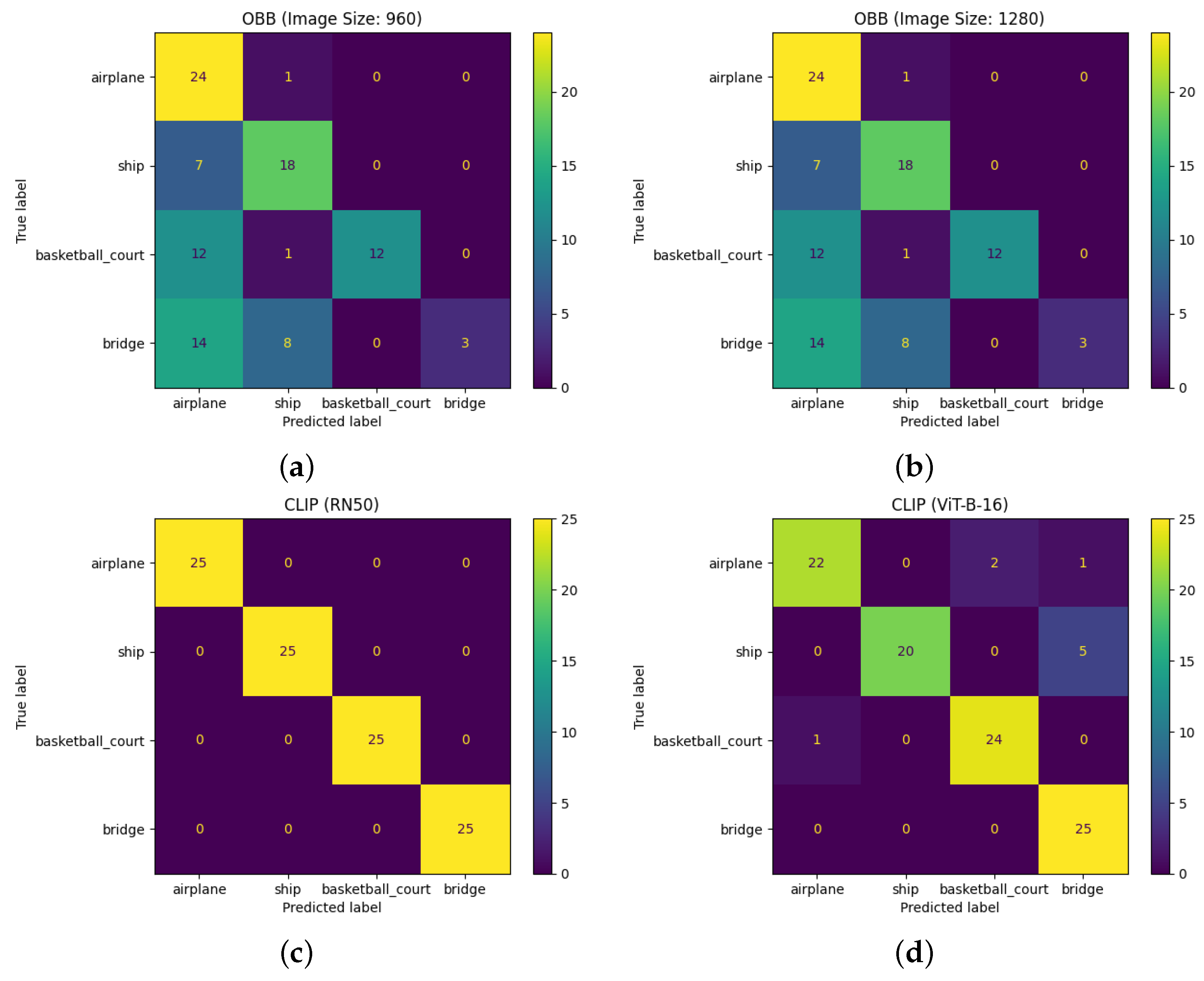
Figure 7 presents the confusion matrices produced from the classifications predicted by the OBB and CLIP approaches. Classifications for a given image were predicted by determining the class description with which it had the highest cosine similarity score. This provided a good indication of the performance of each approach in making correct image–description associations.

The CLIP models performed the best by far, with the ResNet50-based model showing 100% accuracy for classification. Meanwhile, the OBB methods appeared to struggle with the class classifications, perhaps due to the performance of the YOLOv8 models on this dataset. This was especially evident in the “bridge” class, a class on which both YOLOv8 models performed poorly.

The goal of these approaches was to prioritize the downlink of data so that the most desirable data were downlinked first; therefore, it was important to visualize the effect of prioritization on data downlink. Figure 8 presents the simulated effect on the downlink from each approach when a specific class was requested. Prioritization for a given class was performed by sorting the class similarities from high to low and downlinking the images with the highest similarities to the given class first. The perfect case would see the 25 images in a class downlinked within 25 image downlinks.

Figure 8a presents the case of a randomly sorted baseline where no prioritization was applied. An efficiently prioritized result would see a straight line to the total number of images in a class, as no undesirable images were downlinked. Horizontal movement in the plot indicated that the downlink of an image from an undesired class took place. Visually, an improvement in performance can be seen in most cases where prioritization was performed. The most improvement was seen with the CLIP models, specifically with the ResNet50-based model in Figure 8d, with perfect downlink prioritization for almost all classes.

Another method to quantify prioritization performance is to consider the prioritization error, calculated as:

$$ϵ=1-m,$$

(3)

where m is the regression line fit to the plots in Figure 8 using the polyfit function from the Numpy Python library [28]. A lower error means better prioritization performance.

Table 12. Prioritization error.

Model	Airplane	Ship	Basketball_Court	Bridge
No priority	0.77	0.78	0.73	0.62
OBB 960	0.73	0.71	0.77	0.72
OBB 1280	0.73	0.71	0.77	0.72
CLIP RN50	0.00	0.00	0.00	0.24
CLIP ViT-B-16	0.62	0.58	0.03	0.58

presents the prioritization error for the OBB and CLIP approaches for each class in the PrioEval dataset. A baseline case where no prioritization is performed is, once again, provided.

The ResNet50-based CLIP model provided the lowest error rate for all classes, showing that it efficiently prioritized the downlink of RS images. The ViT-B-16-based CLIP model was impacted by sequencing the last few images in each class later on in the downlink process, resulting in a higher prioritization error. The OBB models seemed to perform relatively well on vehicles; however, they too were severely impacted from prioritizing the last few images in a class much later in the downlink process, also resulting in a higher prioritization error.

Finally, the runtime performance and memory requirements of each approach on the VERTECS CCB must be considered.

Table 13. Intermediate representation size.

Associated Model/Approach	Size
OBB	179 B
CLIP RN50	16.38 KB
CLIP ViT-B-16	8.38 KB

presents the size of the intermediate representation files for each approach, which include representations for the four different text class descriptions. These are the files which must be uplinked to the satellite for similarity score calculation. In this case, a smaller file is best, as this would require less bandwidth to uplink to a nanosatellite in orbit.

The OBB approach featured the smallest file size due to being a simple JSON object. The CLIP models had a larger file size as they were text embeddings output by their respective text encoders.

Figure 9 presents the CPU usage, memory usage, maximum memory consumed, and total runtime of each model evaluated on the VERTECS CCB.

The majority of the runtime for both approaches was taken by image processing, with actual similarity score calculation taking a fraction of the time. The average image processing time for a single image and the similarity calculation time for 100 images are presented in

Table 14. Average image processing and similarity calculation times for each model.

Model	Image Processing	Similarity Calculation
	(Seconds/Image)	(Seconds/100 Images)
OBB 960	2.47	0.28
OBB 1280	4.38	0.28
CLIP RN50	0.96	0.003
CLIP ViT-B-16	1.61	0.0006

for each model.

CLIP appeared to process images more efficiently due to processing them as a batch, while for the OBB approach, YOLO needed to make predictions one image at a time. The same was the case for calculating the similarity score as CLIP made one dot product calculation for all images and text descriptions considered, while the OBB approach calculated similarity class-by-class before obtaining an average, performing this one image at a time.

While the OBB approach had lower CPU and memory utilization, the total runtime of the algorithms was longer compared to those of the CLIP approach. This means that the CCB had to operate for a longer time, consuming more power in the process. This is clear in Figure 10, which presents the power consumption over time of the VERTECS CCB, at 5 V, when running the main program code of each approach. A uniform filter was applied over the data to increase the clarity of the plots. While the CLIP approach experienced higher peak power usage, the power consumption over time in watt hours for the CLIP approach was lower compared to that of the OBB approach.

Table 15. Power statistics for each approach running on the VERTECS CCB.

Associated Model/Approach	Max Power (W)	Power Consumption (Wh)
OBB 960	4.54	13.96
OBB 1280	4.69	24.92
CLIP RN50	5.37	7.63
CLIP ViT-B-16	5.59	13.63

presents these values for each variant of each approach. The values show that less energy was consumed overall by running the CLIP algorithms on the VERTECS CCB compared to the OBB algorithms.

Therefore, despite having increased CPU and memory utilization, if the memory requirement can be met, the CLIP approach is more desirable since the required hardware up-time and total power consumption are lower.

4. Discussion

While for evaluation simplicity, the prioritization test performed in this work focused on classification into distinct classes using class descriptions, it should be noted that the benefit of using natural language descriptions over a regular classifier lies in the improved flexibility and granularity provided by natural language descriptions, as well being more intuitive for the end user. It allows for prioritization even when an image does not fall cleanly within a distinct class; however, this is more difficult to test and evaluate given the currently available datasets.

The OBB approach assumes that the extracted OBB descriptions carry enough information to sufficiently characterize an image and that a description can be converted to a comparable form. The performance of this approach is tied to its ability to predict bounding boxes, in this case, the performance of YOLOv8, and the ability to convert descriptions to intermediate representations, in this case, the performance of Llama2. The DOTA-v1.5 dataset is a challenging dataset, as it contains many different objects of various sizes in the same image. While identifying the exact regions inhabited by each object is not that important in this case, it is very important to at least identify every object present and provide a sufficiently accurate center point for each one. At times, YOLOv8 failed to do this sufficiently, even resulting in cases of no detections for certain images. The fact that the descriptions had to be artificially generated also did not help the overall performance of that approach. The artificial descriptions lacked true variety in terms of natural language. However, the results still sufficiently showed that a good comparable intermediate representation could be generated using the Llama2 LLM. Despite its shortcomings, the OBB approach did show promise when considering the top-30 accuracy scores. It appeared to produce outputs which could filter and prioritize images to a sufficient degree to see a slight improvement in the best performing classes. Given improvements in OBB prediction and access to better descriptions, along with a more robust and information dense intermediate representation, the OBB method could prove useful for prioritizing RS images for downlink.

The CLIP approach worked very well for this prioritization task, especially the ResNet50-based model. The structure and approach of CLIP lends itself well to the use-case explored in this paper, with its image and text embeddings providing a good intermediate representation which can be used to determine similarity for later prioritization. This could allow for more flexibility than even the OBB approach. Given access to more data, the performance of the CLIP approach could see further improvement, as much of the performance of CLIP stems from pre-training on large datasets of image–text pairs. While CLIP produced good results and ran within the confines of the target nanosatellite hardware, the model itself is large and requires a significant amount of memory. This will prevent it from running on more constrained systems. Perhaps implementing some form of knowledge distillation, whereby a smaller neural network is trained to replicate the output of a larger network, could reduce the memory requirements, while still maintaining decent performance.

Based on the results presented in Section 3, the viability of the proposed conceptual prioritization pipeline can be confirmed, as the approaches modeled after this pipeline resulted in successful prioritization of the RS images. If natural language-based prioritization needs to be implemented today, the ResNet50-based CLIP approach is by far the best performing approach, considering both performance and runtime, and should be considered. However, as technology improves and more computational resources become available on nanosatellites, perhaps a larger CLIP model trained on more data will perform better.

5. Conclusions

In conclusion, this paper shows that while much work still needs to be done, natural language models can be used to prioritize images on CubeSats with more flexibility compared to existing techniques. Two approaches were proposed to alleviate the strain on nanosatellite operations imposed by data downlink bandwidth limitations. These approaches used the NLP-based prioritization pipeline concept proposed in Figure 1 to improve on the prioritization of CubeSat images implemented by the works discussed in Section 1. This was achieved by allowing images to be prioritized outside of the previously known, discrete classes, with which the models were trained. Given a natural language description of an RS scene, these approaches attempted to find the most similar images stored on-board the satellite and prioritize them for downlink. The first approach made use of YOLOv8 on-board the nanosatellite to produce an intermediate representation derived from OBB predictions to compare against a natural language description processed by Llama2 on the ground. The second approach implemented the ResNet50 and ViT-B-16 versions of CLIP to produce image embeddings on-board the nanosatellite and text embeddings on the ground, which could be compared to find the most similar image given a text description.

In terms of classification and prioritization performance, the ResNet50-based CLIP model performed the best, with a 100% classification accuracy and near perfect prioritization observed during the prioritization test. As for runtime and power performance on the VERTECS CCB, the CLIP approach utilized more of the CPU and required more system memory than the OBB approach, resulting in a higher maximum power draw; however, the CLIP approach experienced a shorter runtime, resulting in less power consumption overall. Of the two CLIP models, the ResNet50-based CLIP model had the shortest runtime and therefore lowest overall power consumption. While all approaches successfully ran on the target hardware, it may not be possible to run the CLIP approach on more resource-constrained systems with less system memory, making the OBB approach favorable for such cases.

Ultimately, the ResNet50-based implementation of CLIP performed the best based on the evaluated metrics and showed that natural language descriptions can be used to prioritize RS image data for downlink.

In the future, further improvements to both approaches could see better results for the RS image prioritization task explored in this work. For the OBB approach, a better OBB predictor and intermediate representation should be implemented to increase prioritization performance, along with providing more varied descriptions for each image. For the CLIP approach, more image–text data pairs of RS scenes should be provided for training to increase performance, while knowledge distillation techniques should be used to reduce the functional model size and memory requirements on the satellite.