Deep Learning-Based Rapid Flow Field Reconstruction Model with Limited Monitoring Point Information

Abstract

The rapid reconstruction of the internal flow field within pressure vessel equipment based on features from limited detection points was of significant value for online monitoring and the construction of a digital twin. This paper proposed a surrogate model that combined Proper Orthogonal Decomposition (POD) with deep learning to capture the dynamic mapping relationship between sensor monitoring point information and the global flow field state during equipment operation, enabling rapid reconstruction of the temperature field and velocity field. Using POD, the order of the tested temperature field was reduced by 99.75%, and the order of the velocity field was reduced by 99.13%, effectively decreasing the dimensionality of the flow field. Our analysis revealed that the first modal coefficient of the temperature field snapshot data, after modal decomposition, had a higher energy proportion compared to that of the velocity field snapshot data, along with a more pronounced marginal effect. This indicates that more modes need to be retained for the velocity field to achieve a higher total energy proportion. By constructing a CSSA-BP model to represent the mapping relationship between the modal coefficients of the temperature and velocity fields and the data collected from the detection points, a comparison was made with the BP method in reconstructing the temperature field of a shell-and-tube heat exchanger. The CSSA-BP method yielded a maximum mean squared error (MSE) of 9.84 for the reconstructed temperature field, with a maximum mean absolute error (MAE) of 1.85. For the velocity field, the maximum MSE was 0.0135 and the maximum MAE was 0.0728. The global maximum errors for the reconstructed temperature field were 4.85%, 3.65%, and 4.29%, respectively. The global maximum errors for the reconstructed velocity field were 17.72%, 11.30%, and 16.79%, indicating that the model established in this study has high accuracy. Conventional CFD simulation methods require several hours, whereas the reconstruction model proposed here can rapidly reconstruct the flow field within 1 min after training is completed, significantly reducing reconstruction time. This work provides a new method for quickly obtaining the internal flow field state of pressure vessel equipment under limited detection points, offering a reference for online monitoring and the development of digital twins for pressure vessel equipment.

1. Introduction

Obtaining the internal flow field characteristics of pressure vessels during operation is of significant value in monitoring equipment performance, developing digital twins, and guiding equipment operation [1,2,3]. Computational Fluid Dynamics (CFD) methods, based on solving discretized nonlinear partial differential equations [4], have become the primary means of studying flow field characteristics. However, in cases requiring multiple iterations for solving, the complexity of the flow field structure, the refinement of the grid, and the accuracy of the solution place higher demands on the speed and timeliness of the solution.

Mapping models between boundary conditions and flow field characteristics have been widely studied based on deep learning methods to achieve rapid flow field prediction. Liu et al. [5] proposed the LAFlowNet model, which used point cloud information to predict instantaneous and average blood flow fields within the heart, addressing the low timeliness of CFD simulations. Kong et al. [6] conducted uniform slicing of three-dimensional flow fields to obtain two-dimensional flow field information and established a convolutional neural network model to predict the Mach number distribution of the combustion chamber flow field using wall pressure conditions. Additionally, the studies by Zhong et al. [7], Guo et al. [8], Jiang et al. [9], Zhou et al. [10], Li et al. [11], and Huang et al. [12] all employed deep learning methods to construct surrogate models between boundary conditions and global flow field characteristics, achieving the rapid prediction of flow fields. However, for flow fields with complex structures and large-scale variations, local flow field features were particularly crucial for diagnosing equipment performance. Building surrogate models for rapid flow field prediction based on boundary conditions or local features often risks losing important local flow field characteristics. Additionally, it involves significant computational effort.

Establishing a reduced-order model (ROM) for unsteady flow fields to simplify the dynamic characteristics representation of flow field systems effectively improved the efficiency of flow field prediction [13,14]. The construction of the reduced-order model is divided into two main stages: model dimension reduction and state reconstruction of the low-dimensional system [15,16]. Commonly used dimension-reduction methods include POD [17,18,19], DMD [20,21], and DL [22,23]. Original datasets were constructed based on experiments or CFD calculations, reduced basis functions were extracted, and the system was projected into a lower-dimensional space. By truncating the higher-order modes after projection, the primary lower-order modes were extracted and linearly superimposed to achieve low-dimensional reconstruction of the flow field [24]. Depending on whether the governing equations were included in the reduced-order model, it could be classified into embedded or non-embedded types [25]. In the embedded approach, Maia I A et al. [26] developed a generalized quasi-linear framework combined with the Galerkin reduced-order model for turbulence prediction. Bhatnagar S et al. [27] proposed a flow field approximation prediction model based on convolutional neural networks to reduce computation time and predict the velocity and pressure fields of airfoils over short time intervals by using shared encoding and decoding layers. Boon W. M. et al. [28] constructed a reduced-order strategy based on deep neural networks to perform reduced-order solving of linearly constrained partial differential equations. Embedded reduced-order methods achieved good accuracy for solving strongly nonlinear flow fields, but they had certain limitations on model input features and were not suitable for online monitoring systems.

In the non-embedded approach, researchers primarily focused on constructing data-driven surrogate models to map local flow field features to lower-order system modes. Dai et al. [29] used spline interpolation to obtain POD coefficients under non-design conditions and established a multiple linear regression model to predict the thermal performance of Reactor Pressure Vessel (RPV) insulation structures. Min et al. [30] employed a POD-RBFNN model to predict flow field data at non-sample points in a nuclear reactor core. Huang et al. [31] constructed a model combining DMD and ConvLSTM for the rapid prediction of flow field states. Saeed A et al. [32] developed a reduced-order model for rapid flow field prediction that combined LSTM with POD. Overall, data-driven reduced-order methods were able to effectively improve flow field prediction efficiency and reduce the computational cost of nonlinear systems.

It is worth noting that the current research mainly focuses on performance prediction during the equipment design phase. By predicting the physical field state under different design conditions, rapid simulations are conducted to guide equipment design. However, during actual operating conditions, the equipment’s performance is influenced by the coupling of multiple factors and exhibits dynamic changes. The real-time information extracted from a limited number of measurement points may be insufficient for accurately assessing the overall state of the equipment. Combining information from limited detection points to comprehensively reconstruct the internal flow field characteristics of the equipment is a key technology for achieving online monitoring of operational status and digital twin modeling, and it warrants further exploration.

This paper introduces a rapid flow field reconstruction model based on deep learning with limited point information. A reduced-order model of the flow field was established using the POD-SVD method, which separated the flow field modes and modal coefficients, achieving dimensionality reduction by decomposing high-dimensional data into modes. A CSSA-BP deep learning neural network model was constructed to capture the dynamic mapping between the low-order flow field modal coefficients and the measurement point data, enabling rapid flow field reconstruction. The developed rapid flow field reconstruction model was validated using a horizontal shell-and-tube heat exchanger as the experimental object. The novelty of this research lies in reducing the dimensionality of the high-dimensional physical field and establishing a surrogate model that maps the measurement point information to the truncated global flow field modal coefficients, which enables rapid flow field reconstruction and online monitoring during equipment operation.

2. Methodology

2.1. Model Reduction Based on POD-SVD

Proper Orthogonal Decomposition (POD) obtains multiple sets of low-dimensional optimal bases from a large set of experimental or simulation data. POD combines these optimal bases to approximate the original complex system, achieving dimension reduction [4,33,34]. For unsteady flow fields, the physical field characteristics at a given moment can be recorded as a snapshot, and snapshots from different times are then assembled to form the physical field dataset U(m,N), as shown in Equation (1):

$${\left[U\right]}_{m\times N}=\left[\begin{array}{llll}{u}_{1,1}& u_{1,2}& \cdots & u_{1,N}\\ u_{2,1}& u_{2,2}& \cdots & u_{2,N} \\ ⋮& ⋮& \ddots & ⋮\\ u_{m,1}& u_{m,2}& \cdots & u_{m,N}\end{array}\right]$$

(1)

where m represents the number of sampling points, N denotes the number of snapshots, and $U\left(m,N\right)$ is referred to as the snapshot matrix of the original physical field.

According to POD theory [35], the snapshot matrix is decomposed into the sum of the mean matrix $U_0$ and the fluctuating matrix $U^{\prime }$, as shown in Equation (2):

$$U(m,N)=U_0+U^{\prime }$$

(2)

The mean matrix $U_0$ is calculated as follows:

$$U_0={\displaystyle \frac{{\displaystyle \sum _{i=1}^{N}U(m,N)}}{N}}$$

(3)

Using the method of separation of variables, the fluctuation matrix $U^{\prime }\left(m,N\right)$ can be decomposed into POD basis vectors and modal coefficients, as shown in Equation (4):

$$U^{\prime }(m,N)={\displaystyle \sum _{i=1}^N{a_{i,}}_j}{\phi }_i\hspace{1em}\hspace{1em}i=1,2,3\cdots N$$

(4)

where ${\phi }_i$ represents the POD basis vectors and $a_{i,j}$ denotes the modal coefficients.

By extracting the key features of the system’s evolution and using a small number of optimal modes to reconstruct complex physical processes, typically, only the first A modes are used for flow field approximation. Therefore, Equation (4) is rewritten as Equation (5):

$$U^{\prime }(m,N)\approx {\displaystyle \sum _{i=1}^A{a_i}_{,j}}{\phi }_i=\widehat{U}(m,N)$$

(5)

where $\widehat{U}\left(m,N\right)$ represents the approximate deviation matrix of the fluctuation matrix.

Therefore, the problem of using POD to describe flow field modal variations becomes one of determining the A-order modes ${\phi }_i$ and modal coefficients $a_{i,j}$. To ensure the accuracy of the mode truncation process, an error expression is constructed. The error between the truncated orthogonal modes and the fluctuation matrix can be expressed as Equation (6):

$$\begin{array}{ll}error& =\left[{\left(U^{\prime }(m,N)-\widehat{U}(m,N)\right)}^T.\left(U^{\prime }(m,N)-\widehat{U}(m,N)\right)\right]\\ & =\left[{\left({\displaystyle \sum _{i=A+1}^N{a}_{i,j}}{\phi }_i\right)}^T.\left({\displaystyle \sum _{i=A+1}^N{a}_{i,j}}{\phi }_i\right)\right]\\ & ={{\displaystyle \sum _{i=A+1}^N{a}_{i,j}}}^2\end{array}$$

(6)

Utilizing the orthogonality between the proper orthogonal modes, Equation (7) can be obtained:

$$a={\phi }^T{U}^{\prime }$$

(7)

The truncation error can be rewritten as shown in Equation (8):

$$\begin{array}{ll}error& =\left[\left({\displaystyle \sum _{i=N+1}^{\infty }{{\phi }_i}^T{U}^{\prime }{U^{\prime }}^T{\phi }_i}\right)\right]\\ & ={\displaystyle \sum _{i=N+1}^{\infty }{{\phi }_i}^T\left(U^{\prime }{U^{\prime }}^T\right)}{\phi }_i\end{array}$$

(8)

Let $R=\left(U^{\prime }{U}^{\prime T}\right)$, where R is a real symmetric matrix. The truncation error can be expressed as:

$$error={\displaystyle \sum _{i=N+1}^{\infty }{{\phi }_i}^{T}R}{\phi }_i$$

(9)

Thus, the problem of finding the optimal set of modes can be transformed into minimizing the truncation error while ensuring the orthogonality of the mode set. Using the Lagrange multiplier method, we introduce the Lagrange multiplier ${\lambda }_i$ and construct the Lagrangian function as follows:

$$L({\phi }_i)={\displaystyle \sum _{i=N+1}^{\infty }{{\phi }_i}^{T}R{\phi }_i}-{\displaystyle \sum _{i=N+1}^{\infty }{\lambda }_i\left({{\phi }_i}^T{\phi }_i-1\right)}$$

(10)

To find the extrema, set ${\displaystyle \frac{d}{d{\phi }_i}}L\left({\phi }_i\right)=0$, which yields:

$${{\phi }_i}^{T}R{\phi }_i={\lambda }_i$$

(11)

From Equation (11), it can be seen that the Lagrange multiplier ${\lambda }_i$ represents the eigenvalues of the real symmetric matrix $R$ and ${\phi }_i$ represents the eigenvectors of the real symmetric matrix $R$. Using the properties of real symmetric matrices, all eigenvalues of the matrix $R$ are real numbers, and the eigenvectors are mutually orthogonal. Thus, the truncation error can be expressed as:

$$error={\displaystyle \sum _{i=A+1}^N{{\phi }_i}^{T}R}{\phi }_i={\displaystyle \sum _{i=A+1}^N{\lambda }_i}$$

(12)

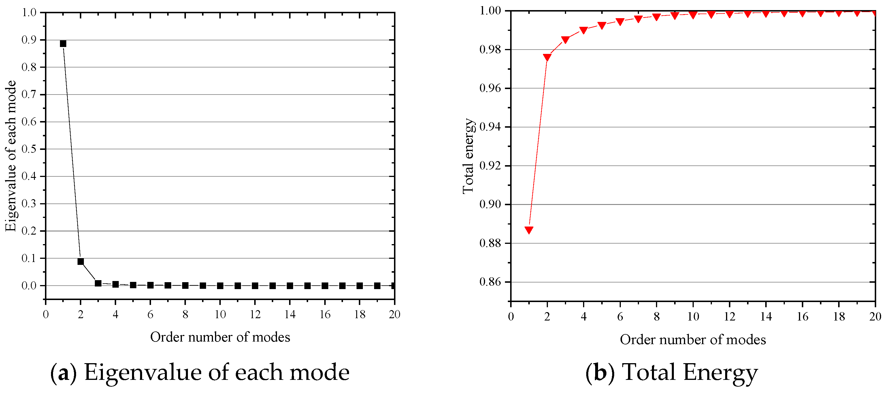
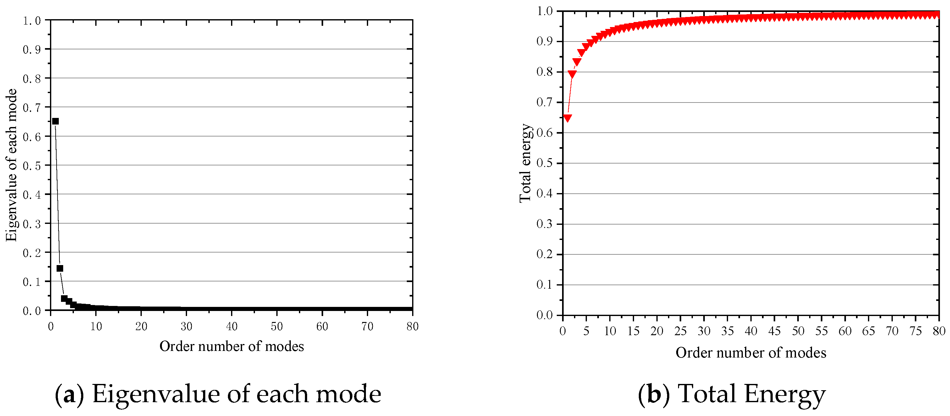
To minimize the truncation error, the eigenvalues ${\lambda }_i$ are arranged in descending order, and the top N largest eigenvalues are selected. The eigenvectors corresponding to these eigenvalues constitute the optimal orthogonal mode set for POD. The selection rule is as follows:

$$E_A={\displaystyle \frac{{\displaystyle {\sum }_{i=1}^A{\lambda }_i}}{{\displaystyle {\sum }_{i=1}^N{\lambda }_i}}}\ge \gamma ,\hspace{1em}\hspace{1em}A<N$$

(13)

where $\gamma$ represents the proportion of energy retained in the original mode set by the orthogonal mode set after truncation.

Based on the orthogonality of eigenvectors, the Singular Value Decomposition (SVD) [36] method can simplify the solution process. By applying SVD, the matrix in Equation (2) is decomposed into three distinct matrices, namely:

$$\left[B,S,V\right]=SVD\left(U^{\prime }\right)$$

(14)

where $B\in R^{m\times m}$, $S\in R^{m\times N}$, $V\in R^{N\times N}$, B is the matrix containing the standard orthogonal eigenvectors of $U^{\prime }\left(x,t\right)U^{\prime }{(x,t)}^T$, and is therefore referred to as the mode construction matrix. S is a diagonal matrix consisting of singular values arranged in descending order, and V represents the spatial modes.

The POD basis vectors ${\phi }_i$ are solved according to Equation (15):

$${\phi }_i=V$$

(15)

the modal coefficients $a$ are solved according to Equation (16):

$$a=B.S$$

(16)

the energy of each mode, represented by the eigenvalues ${\lambda }_i$ of the characteristic matrix R, is solved according to Equation (17):

$${\lambda }_i={S_i}^2$$

(17)

for a given snapshot matrix U, the POD basis vectors ${\phi }_i$ extracted through POD decomposition are constants. In a nonlinear flow field, the modal coefficients $a_i$ can be considered to have some implicit relationship with the local measurement points.

2.2. CSSA Improve BP

By utilizing neural network algorithms, a nonlinear transfer model between modal coefficients $a_i$ and detection point features was established. The Backpropagation Neural Network (BPNN) provides high versatility and adaptability and its objective function is:

$$E={\displaystyle \frac{1}{2\times N_t}}{\displaystyle \sum _{P=1}^P{\displaystyle \sum _{q=1}^Q\left(y_{p.q}{\widehat{y}}_{p.q}\right)}}$$

(18)

where $N_t$ represents the number of training samples, P denotes the number of neurons in the input layer, Q is the dimension of the input variable y, $y_{p.q}$ is the predicted value, and ${\widehat{y}}_{p.q}$ is the actual value.

The relationship between the input and output of a neuron can be represented by an activation function $\sigma$:

$$y_j=\sigma \left({\displaystyle \sum _{i=1}^n{w}_{ij}\times c_i+b_j}\right)$$

(19)

where $y_j$ represents the output of the $j$th neuron in the hidden layer, $c_i$ represents the input to the $i$th neuron, $w_{ij}$ denotes the weight coefficient, $b_j$ is the bias value of the neuron, and $n$ represents the number of neurons in the previous layer.

In order to determine the network structure and address issues such as the algorithm easily getting trapped in local optima and slow convergence speed, the Chaotic Sparrow Search Algorithm (CSSA) was employed for optimization. In SSA, a matrix was used to represent the position coordinates of virtual sparrows during the food search process:

$$X=\left[\begin{array}{cccc}{x}_{1,1}& x_{1,2}& \cdots \cdots & x_{1,d}\\ x_{2,1}& x_{n,2}& \cdots \cdots & x_{2,d}\\ ⋮& ⋮& \ddots & ⋮\\ x_{n,1}& x_{n,2}& \cdots \cdots & x_{n,d}\end{array}\right]$$

(20)

where $x_{id}$ represents the position of the sparrow in space. The sparrow’s foraging process was abstracted into a producer–joiner model, where the producer updated its position using the following equation:

$$X_{i,j}^{t+1}=\{\begin{array}{ll}{X}_{i,j}^t.\exp \left({\displaystyle \frac{-i}{\alpha .ite{r}_{\max }}}\right)& if R_2<ST\\ X_{i,j}^t+Q.L& if R_2\ge ST\end{array}$$

(21)

where $t$ represents the current iteration count, $T$ is the maximum number of iterations, $\alpha$ is a uniform random number between [0, 1], $Q$ is a random number following a normal distribution, $L$ is a matrix of size $1\times d$ with all elements equal to 1, and $R_2\in \left[0,1\right]$ and $ST\in (0.5,1]$ represent the warning and safety values, respectively. When $R_2<ST$, it indicates that the population has not detected the presence of predators or other dangers, guiding the population to achieve higher fitness. Conversely, when $R_2\ge ST$, the scouting sparrow detects a predator and immediately releases a danger signal, prompting the population to adjust its search strategy and move towards a safer area.

Sparrows other than the producers, acting as joiners, updated their positions using the following equation:

$$X_{id}^{t+1}=\{\begin{array}{l}Q.\exp \left({\displaystyle \frac{x{w}_d^t-x_{id}^t}{i^2}}\right) , i>{\displaystyle \frac{n}{2}}\\ x{b}_d^{t+1}+{\displaystyle \frac{1}{D}}{\displaystyle \sum _{d=1}^D\left(rand\left\{-1,1\right\}.\left|x_{id}^t-x{b}_d^{t+1}\right|\right)},i\le {\displaystyle \frac{n}{2}}\end{array}$$

(22)

where $x{w}_d^t$ represents the worst position of the sparrow in the d-dimensional space during the t-th iteration of the population; $x{b}_d^{t+1}$ represents the best position of the sparrow in the d-dimensional space during the $t+1$-th iteration; when $i\ge n/2$, it indicates that an i-th joiner did not obtain food, resulting in low fitness, and needs to search for food elsewhere; when $i\le n/2$, the i-th joiner randomly searches for food near the current optimal position $xb$.

The position of the scouting sparrow is updated according to the following equation:

$$X_{id}^{t+1}=\{\begin{array}{l}x{b}_d^{t+1}+\beta \left(x_{id}^t-x_d^t\right) , f_i\ne f_g\\ x{b}_{id}^t+K\left({\displaystyle \frac{x_{id}^t-x{w}_d^t}{\left|f_i-f_w\right|+e}}\right) , f_i=f_g\end{array}$$

(23)

where $\beta$ represents the step size control parameter, which follows a normal distribution with a mean of 0 and a variance of 1; $K$ is the step size control parameter; $K\in \left[-1,1\right]$; $e$ is a very small constant; $f_i$ is the fitness value of an individual; $f_g$ and $f_w$ represent the best and worst fitness values in the population, respectively.

To prevent the SSA from getting trapped in local optima and to increase population diversity, Tent chaotic perturbation was introduced, which carries the chaotic variables into the solution space:

$$new{X}_d=mi{n}_d+(ma{x}_d-mi{n}_d).Z_d$$

(24)

where $mi{n}_d$ and $ma{x}_d$ represent the maximum and minimum values of the $d$-dimensional variable $new{X}_d$.

The individual chaotic disturbance was applied according to the following equation:

$$new{X}^{\prime }=(X^{\prime }+newX)/2$$

(25)

where $X^{\prime }$ represents the individual requiring chaotic disturbance, $newX$ is the generated chaotic disturbance, and $new{X}^{\prime }$ is the individual after chaotic disturbance.

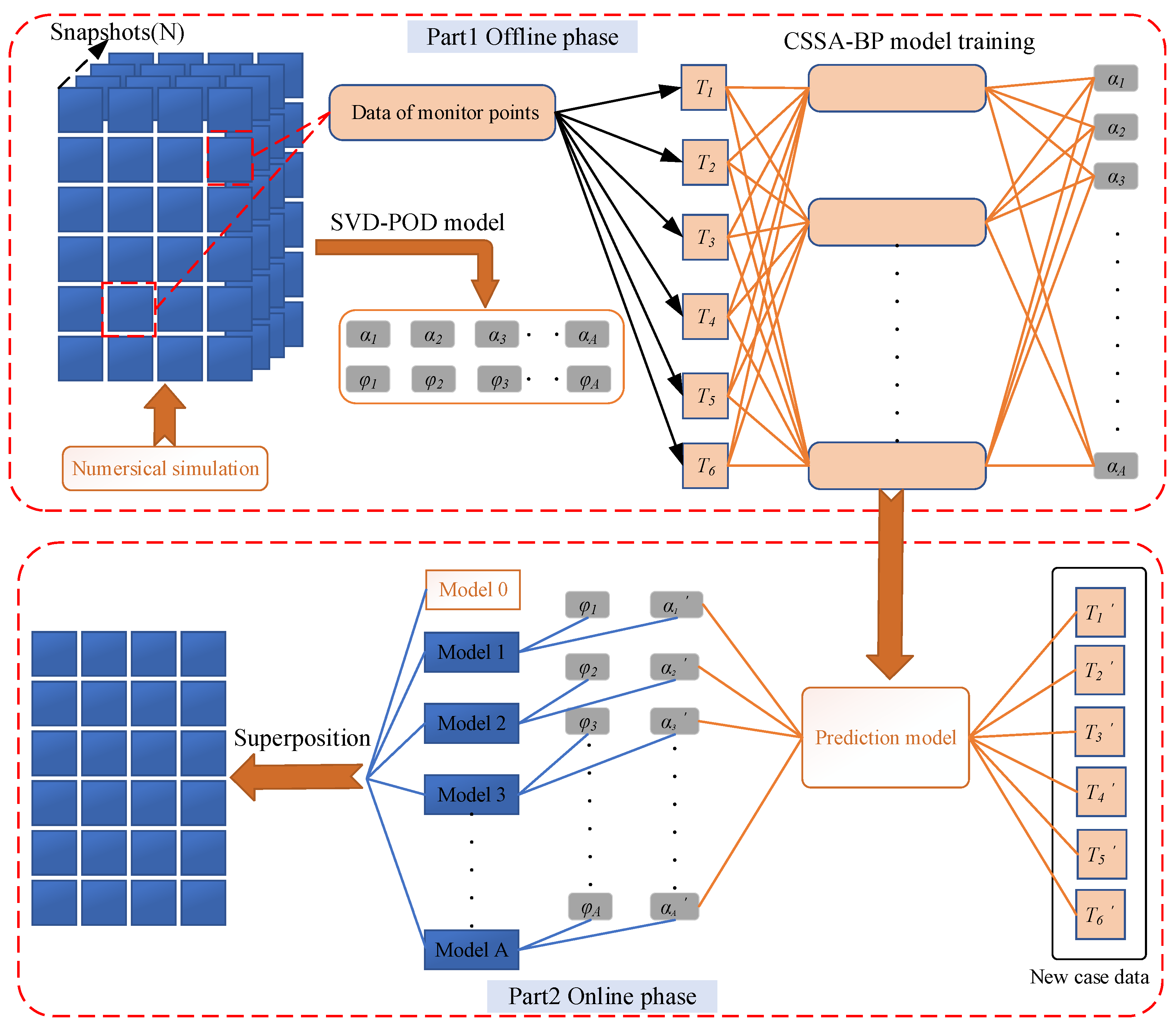
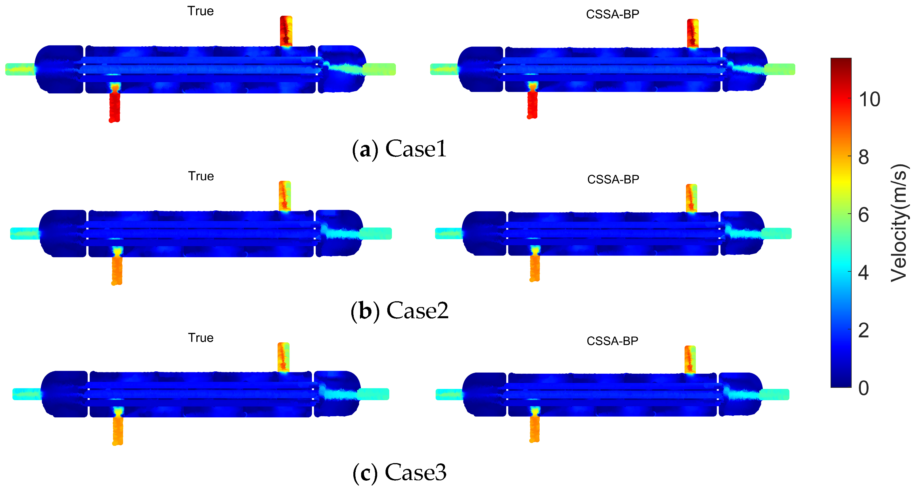
2.3. Flow Field Rapid Reconstruction Model Based on Limited Detection Point Information

Based on the SVD-POD method introduced in Section 2.1 and the CSSA-BP method introduced in Section 2.2, a data-driven deep learning model can be established for the rapid reconstruction of flow field states, as shown in Figure 1.

The model can be divided into two parts:

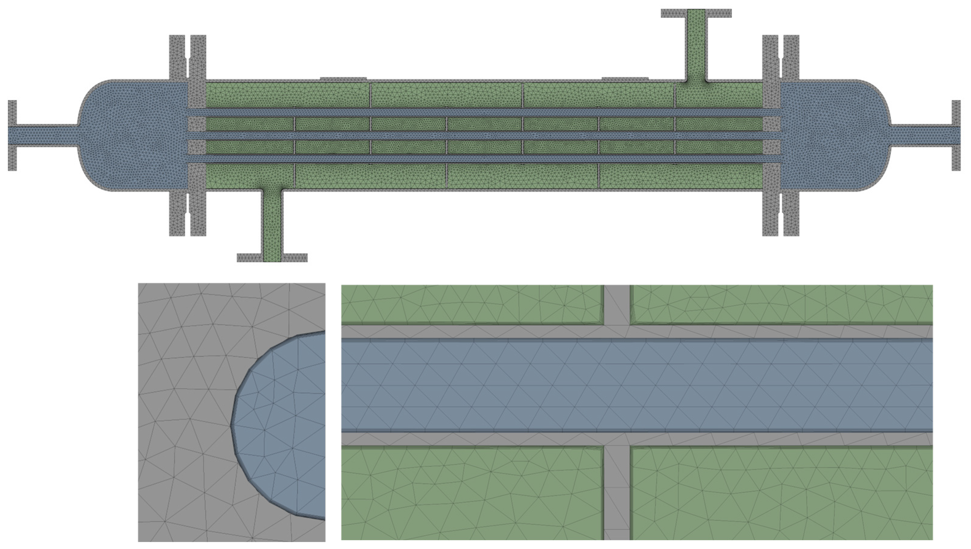
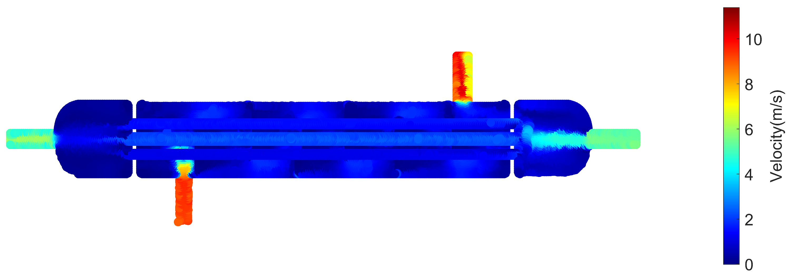
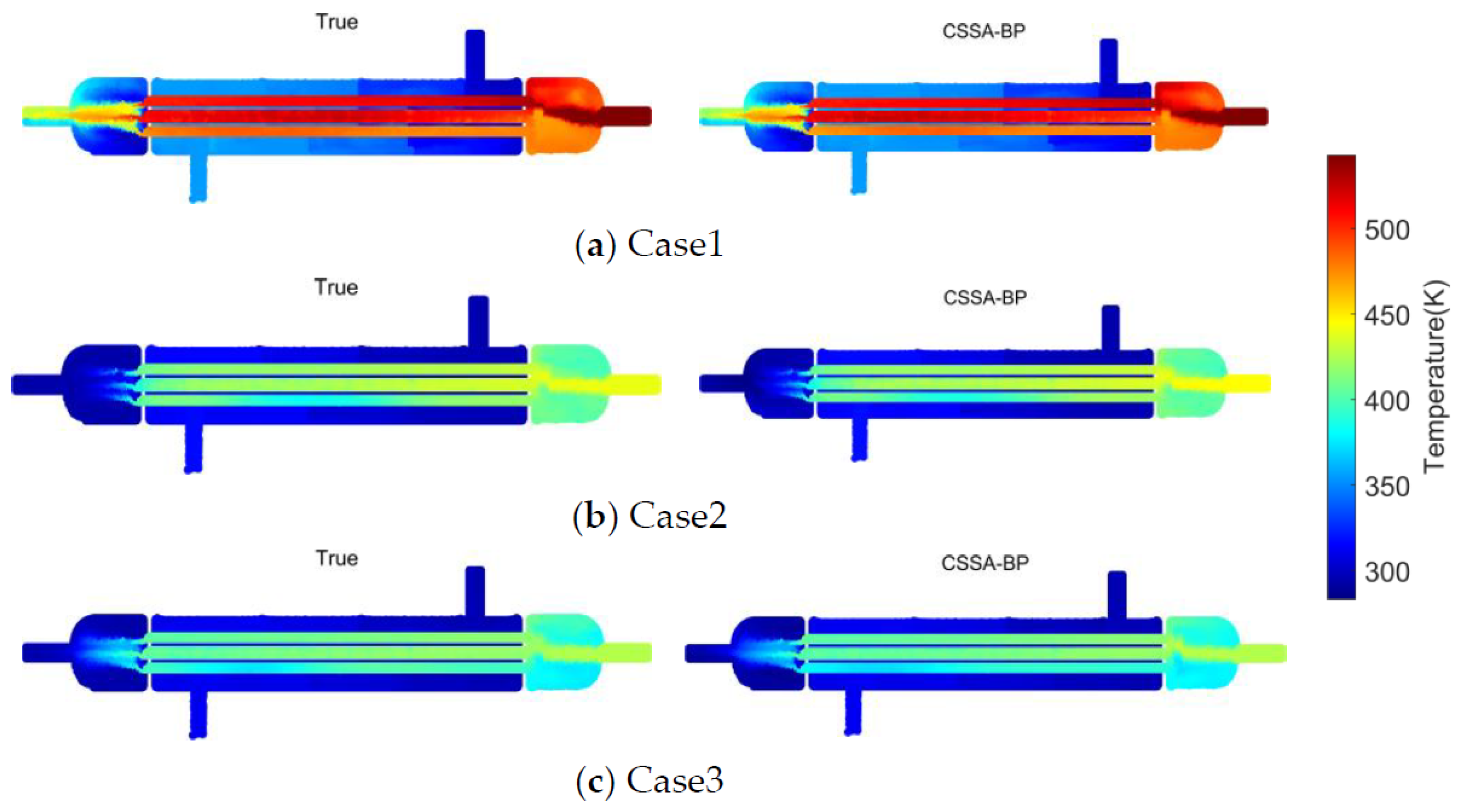
Offline phase: Based on different operating conditions of the equipment, a series of numerical simulations of the flow field were conducted. Representative planes were extracted from the CFD simulation results to construct snapshot data. The SVD-POD method was then used to perform modal decomposition on the snapshot matrix, resulting in POD modes and corresponding feature coefficients. The average mode of the flow field was extracted, and the top A modes were selected based on the truncated modal energy ratio requirement to approximate the dynamic characteristics of the physical system. Detection point data were extracted and combined with the top A-order POD modal coefficients to train a CSSA-BP model, which established a surrogate relationship between the detection point data and the global flow field state.

Online Phase: When the equipment operates under new working conditions, information from the detection points is obtained and input into the trained neural network. This allows for the rapid acquisition of flow field modal coefficients under the new conditions. The deterministic POD modes obtained during the offline phase are linearly combined with the characteristic coefficients predicted by the CSSA-BP model and then superimposed with the average flow field mode to quickly reconstruct the flow field.

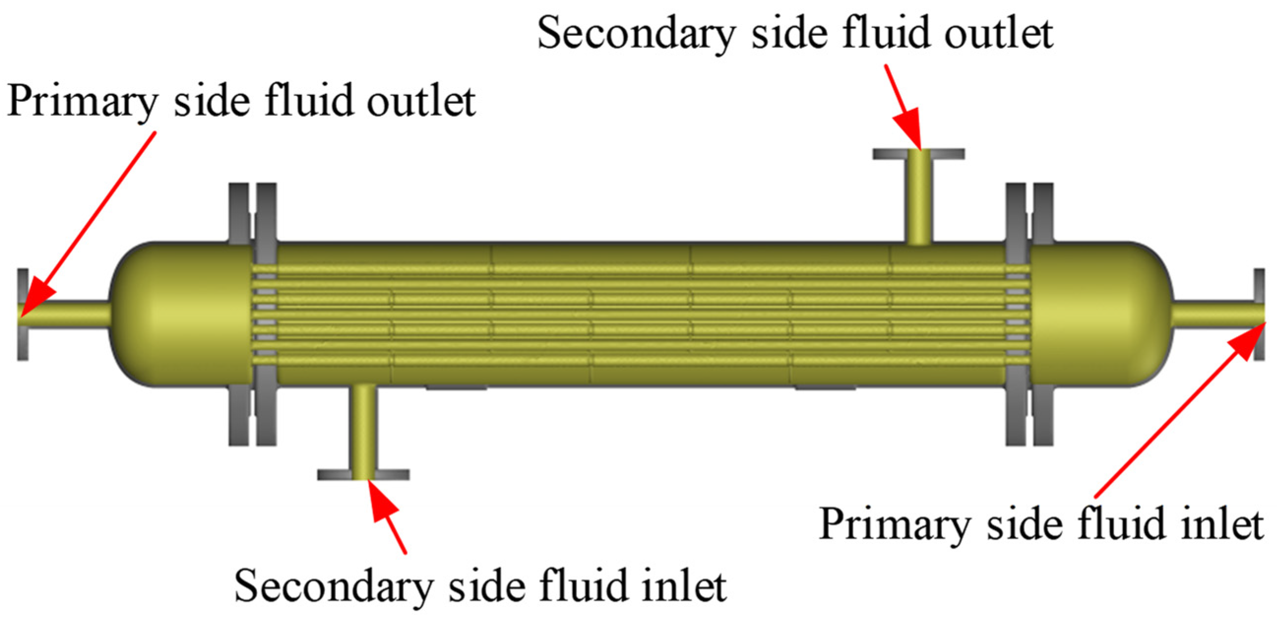
Through these steps, the dimensionality of the flow field system is reduced, enabling the rapid reconstruction of the physical field inside the pressure vessel. This provides a foundation for the online monitoring of pressure vessel equipment and the development of digital twins.

3. Generate Database

3.1. Case Description

Using a typical horizontal shell-and-tube heat exchanger, this study validates the proposed flow field rapid reconstruction model. In this heat exchanger, air and flue gas are used for heat exchange, primarily in waste heat recovery from exhaust gases in the metallurgical industry to improve energy efficiency. The primary-side fluid is high-temperature flue gas, while the secondary-side fluid is air.

During the operation of the heat exchanger, the heat transfer flow field inside the shell serves as a key indicator for assessing the health characteristics of the equipment and guiding its maintenance and repair. However, in industrial applications, the health status of the equipment is mainly estimated through a limited number of sensor detection points. Therefore, developing a digital twin model for the heat exchanger to accurately represent its health status has become a current research focus. Nonetheless, a primary challenge remains, namely, determining how to quickly reconstruct the internal flow field of the heat exchanger using limited detection point information.

The main structure of the heat exchanger consists of a shell, tube sheet, tube bundle, and end cover, with the tube sheet also serving as a flange and without an expansion joint structure. The operating principle of the heat exchanger is illustrated in Figure 2. The primary-side fluid enters through a side inlet, flows through the heat exchange tubes, and transfers heat to the secondary fluid. The secondary-side fluid enters through a bottom inlet and exits from a top outlet. As the secondary fluid flows through the gaps in the tube bundle, it is heated by the primary-side fluid. The main structural parameters of the heat exchanger are presented in

Table 1. Geometrical parameters.

	Quantity	Value
1	Diameter of heat exchange tubes	φ14 mm
2	Number of heat exchange tubes	32
3	Arrangement of heat exchange tube rows	Triangular arrangement
4	Spacing between heat exchange tubes	19 mm
5	spacing between baffle plates	108 mm
6	number of baffle plates	6
7	outer diameter of shell	φ159 mm
8	inner diameter of shell	φ151 mm
9	length of shell	790 mm
10	diameter of primary side connecting pipe	φ25 mm
11	diameter of secondary side connecting pipe	φ25 mm

.

3.2. Fluid Mechanic and Turbulent Flow Equations

The solution was obtained using ANSYS Fluent software, employing Reynolds-averaged Navier–Stokes (RANS) equations to describe the flow characteristics of the primary and secondary side fluids in the heat exchanger. The equations are as follows [37]:

$${\displaystyle \frac{\partial {\overline{u}}_i}{\partial x_i}}=0$$

(26)

$$\rho \left[{\overline{u}}_j{\displaystyle \frac{\partial {\overline{u}}_i}{\partial x_j}}\right]=-{\displaystyle \frac{\partial \overline{P}}{\partial x_i}}\left[\mu \left({\displaystyle \frac{\partial {\overline{u}}_i}{\partial {\overline{x}}_j}}\right)-\rho \overline{u_i^{\prime }{u}_j^{\prime }}\right]$$

(27)

$$\rho c_p{\overline{u}}_j{\displaystyle \frac{\partial \overline{T}}{\partial x_j}}={\displaystyle \frac{\partial }{\partial x_j}}\left[\lambda \left({\displaystyle \frac{\partial \overline{T}}{\partial {\overline{x}}_j}}\right)-\rho \overline{u_j^{\prime }{T}^{\prime }}\right]$$

(28)

The flow field in the heat exchanger follows the conservation of mass, momentum, and energy, defined by the following transport equations [38]:

$${\displaystyle \frac{\partial }{{\partial }_t}}\left(\rho \varphi \right)+{\displaystyle \frac{\partial }{{\partial }_{xj}}}\left(\rho .U\varphi \right)={\displaystyle \frac{\partial }{\partial x_j}}\left({\Gamma }_{\varphi }{\displaystyle \frac{\partial \varphi }{\partial x_j}}\right)+S_{\varphi }$$

(29)

$$\begin{array}{l}{\displaystyle \frac{\partial }{{\partial }_t}}\left(\rho U\right)+div\left(\rho .U.U\right)=div\left({\mu }_{eff}.gradU\right)-{\displaystyle \frac{{\partial }_p}{{\partial }_x}}+{\displaystyle \frac{\partial }{{\partial }_x}}\left({\mu }_{eff}.{\displaystyle \frac{{\partial }_U}{{\partial }_x}}\right)\\ +{\displaystyle \frac{\partial }{{\partial }_y}}\left({\mu }_{eff}.{\displaystyle \frac{\partial V}{{\partial }_x}}\right)+{\displaystyle \frac{\partial }{{\partial }_z}}\left({\mu }_{eff}.{\displaystyle \frac{\partial W}{{\partial }_x}}\right)\end{array}$$

(30)

$$\begin{array}{l}{\displaystyle \frac{\partial }{{\partial }_t}}\left(\rho V\right)+div\left(\rho .V.V\right)=div\left({\mu }_{eff}.gradV\right)-{\displaystyle \frac{{\partial }_p}{{\partial }_y}}+{\displaystyle \frac{\partial }{{\partial }_x}}\left({\mu }_{eff}.{\displaystyle \frac{{\partial }_U}{{\partial }_y}}\right)\\ +{\displaystyle \frac{\partial }{{\partial }_y}}\left({\mu }_{eff}.{\displaystyle \frac{\partial V}{{\partial }_y}}\right)+{\displaystyle \frac{\partial }{{\partial }_z}}\left({\mu }_{eff}.{\displaystyle \frac{\partial W}{{\partial }_y}}\right)\end{array}$$

(31)

$$\begin{array}{l}{\displaystyle \frac{\partial }{{\partial }_t}}\left(\rho W\right)+div\left(\rho .W.W\right)=div\left({\mu }_{eff}.gradW\right)-{\displaystyle \frac{{\partial }_p}{{\partial }_z}}+{\displaystyle \frac{\partial }{{\partial }_x}}\left({\mu }_{eff}.{\displaystyle \frac{\partial U}{{\partial }_z}}\right)\\ +{\displaystyle \frac{\partial }{{\partial }_y}}\left({\mu }_{eff}.{\displaystyle \frac{\partial V}{{\partial }_z}}\right)+{\displaystyle \frac{\partial }{{\partial }_z}}\left({\mu }_{eff}.{\displaystyle \frac{\partial W}{{\partial }_z}}\right)\end{array}$$

(32)

where $\partial /{\partial }_t\left(\rho \varnothing \right)$ is a symbol of the flow exchange rate, $\partial /\partial x_j\left(\rho .U\varnothing \right)$ is considered the flow of convection, the flow of diffusion is shown as $\partial /\partial x_j\left(\Gamma \varnothing \left(\partial \varnothing /\partial x_j\right)\right)$, and ${\mathrm{S}}_{\varnothing }$ is the source term in the former equations.

The flow regime of the fluid within the heat exchanger is confirmed using the Reynolds number $R_e$, calculated using the following formula:

$$R_e={\displaystyle \frac{\rho vD}{\mu }}$$

(33)

where $\rho$ is the density of the fluid, $v$ is the characteristic velocity of the fluid, $D$ is the characteristic length (typically the diameter of the pipe in pipe flow), and $\mu$ is the dynamic viscosity of the fluid.

In the case studied in this paper, the maximum Reynolds number is calculated to be approximately 6800 based on the boundary conditions, indicating that the flow field is turbulent. The standard $k-\epsilon$ model is used to solve the turbulence model, and the equations for turbulent kinetic energy and dissipation rate are as follows:

$$\rho {\displaystyle \frac{dk}{dt}}={\displaystyle \frac{\partial }{\partial x_i}}\left[\left(\mu +{\displaystyle \frac{{\mu }_t}{{\sigma }_k}}\right){\displaystyle \frac{\partial k}{\partial x_i}}\right]+G_k+G_b-\rho \epsilon -Y_M$$

(34)

$$\rho {\displaystyle \frac{d\epsilon }{dt}}={\displaystyle \frac{\partial }{\partial x_i}}\left[\left(\mu +{\displaystyle \frac{{\mu }_t}{{\sigma }_{\epsilon }}}\right){\displaystyle \frac{\partial \epsilon }{\partial x_i}}\right]+C_{1\epsilon }{\displaystyle \frac{\epsilon }{k}}\left(G_k+G_{3\epsilon }{G}_b\right)-G_{\epsilon }\rho {\displaystyle \frac{{\epsilon }^2}{K}}$$

(35)

where $Gk$ represents the production of turbulent kinetic energy, $YM$ accounts for the effects of compressibility on the total dissipation rate, and $C_{1\epsilon }$, $C_{2\epsilon }$, and $C_{3\epsilon }$ are constants. ${\sigma }_k$ and ${\sigma }_{\epsilon }$ are Prandtl numbers, the empirical coefficients are shown in

Table 2. Values and constants of standard k-ε model.

${\mathit{C}}_{\mathit{\mu }}$	${\mathit{C}}_{1\mathit{\epsilon }}$	${\mathit{C}}_{2\mathit{\epsilon }}$	${\mathit{C}}_{3\mathit{\epsilon }}$	${\mathit{\sigma }}_{\mathit{k}}$	${\mathit{\sigma }}_{\mathit{\epsilon }}$
0.09	1.44	1.92	1.44	1	1.3

. While $u_t$ denotes the turbulent viscosity, described by the following formula:

$${\mu }_t=\rho C_{\mu }{\displaystyle \frac{k^2}{\epsilon }}$$

(36)

3.3. Meshing and Model Design

The flow field model of the heat exchanger is symmetric along the 180° axis. A CFD model was established based on a 1/2 model structure, and a tetrahedral structured mesh was generated, with mesh refinement applied at the interface between different structures to ensure a mesh skewness of less than 0.8. Boundary layer meshes were added to the pipes and the fluid–solid interfaces to capture the flow characteristics near the solid walls. The boundary layer was defined with 10 layers, a growth factor of 1.1, and an initial layer thickness of 0.029 mm. The mesh quality was assessed using skewness and orthogonal quality criteria, which can be evaluated in ANSYS Fluent. In the mesh generation described above, the average skewness and orthogonal quality were approximately 0.22 and 0.77, respectively, indicating high mesh quality. The mesh model parameters are shown in

Table 3. Mesh model parameters.

	Quantity	Value
1	Element type	Tetrahedral element
2	Number of elements	5,962,227
3	Number of nodes	2,265,093
4	Average skewness	0.22
5	Average orthogonal quality	0.77

, and the mesh was generated as shown in Figure 3.

With velocity inlet and pressure outlet boundary conditions, the shell-side and tube-side walls are defined as no-slip boundaries. The tube bundle, hot and cold fluids, and shell contact surfaces are all defined as coupled wall heat transfer surfaces, while the outer shell surface is defined for natural convection heat transfer with air. During the simulation, the ambient temperature was considered constant at 20 °C. Based on the physical properties of the problem, our study only accounted for conduction and convection heat transfer, thereby excluding radiation heat transfer effects. The heat transfer between the fluid and the solid heat transfer surfaces was defined as conjugate heat transfer. Considering the structure of the heat exchanger, the number of mesh elements, and other factors, the SIMPLE algorithm was used to discretize the velocity and pressure terms in the momentum equations. A second-order upwind scheme was employed to discretize the equations for energy, momentum, continuity, and turbulence.

The tube bundle area is where the physical field of the heat exchanger changes most dramatically and is also the area of greatest concern in CFD simulation and engineering practice. This study selects the symmetrical plane of the heat exchanger, as shown in Figure 3, for reduced-order model research.

3.4. Validation of CFD Model

To enhance the credibility of the CFD model used in this paper, a comparison was made between the temperatures collected during the actual operation of a heat exchanger on the multifunctional experimental platform at Sichuan University of Science and Engineering under the same operating conditions. This experimental platform mainly consists of a fixed tube sheet heat exchanger, a heating furnace, a centrifugal pump, a water storage tank, a central control console, and various sensors. The structure of the experimental platform is shown in Figure 4, while the validation operating conditions are shown in

Table 4. Validation operating conditions.

Cases	Primary Side Inlet Velocity (m/s)	Primary Side Inlet Pressure (Mpa)	Primary Side Inlet Temperature (K)	Secondary Side Inlet Pressure (Mpa)	Secondary Side Inlet Velocity (m/s)	Secondary Side Inlet Temperature (K)
1	2.6497	0.008	330.39	0.387	4.2191	297.34
2	2.6497	0.007	333.08	0.390	4.3210	296.92
3	2.6497	0.008	336.97	0.393	4.4229	296.51
4	2.6497	0.009	344.14	0.396	4.5045	297

.

The experimental steps are as follows: Start the fuel oil furnace and the industrial control computer; then, enter the experimental program; open the valve to allow the cold fluid to flow through the shell side of the heat exchanger and return to the water tank through the regulating valve, while the hot fluid simultaneously flows through the tube side of the heat exchanger; next, open the tap water valve and rotate the exhaust valve of the cold-water pump to vent any trapped air; once all the air has been vented from the pump, close the exhaust valve; select the variable frequency operation mode for the cold-water pump, start it, and adjust the pressure and flow rate; then, start the hot-water pump and adjust its pressure and flow rate; record the outlet temperature of the cold fluid and the outlet temperature of the hot fluid every 1 s. The experimental data show that the outlet temperatures of the hot and cold fluids stabilize after approximately 150 s, so data are recorded for 150 s for each experimental group. The comparison of simulated and experimental outlet temperatures is illustrated in Figure 5.

From Figure 5, it can be seen that the trend of the CFD temperature values matches that of the measured temperature values under the four experimental conditions. The maximum relative error at corresponding time points is 5%, indicating that the CFD results are in good agreement with the experimental results and demonstrating that the CFD model used in this paper has a high degree of accuracy.

3.5. Conditions of Snapshot Data

The material of the heat exchanger shell is Q345R, with flue gas as the primary-side fluid and air as the secondary-side fluid.

Table 5. Thermal and physical properties of materials [39].

	Quantity	Value
1	Flue gas density (kg/m3)	1.1
2	Flue gas specific heat (J/kg K)	1190.6
3	Flue gas thermal conductivity (W/m K)	0.031
4	Air density (kg/m3)	1.225
5	Air specific heat (J/kg K)	1006.43
6	Air thermal conductivity (W/m K)	0.242
7	Q345R density (kg/m3)	7850
8	Q345R specific heat (J/kg K)	461
9	Q345R thermal conductivity (W/m K)	53.2

presents the physical properties of the materials.

Six parameters, including the inlet temperature, pressure, and flow rate on both the primary and secondary sides, were selected as CFD input conditions. Based on the operating conditions of the heat exchanger shown in

Table 6. Heat exchanger operating parameters.

Boundary	Parameters	Operating Range
Primary side inlet	Temperature (K)	384.05–658.05
	Pressure (Mpa)	0.679–1.213
	Flow velocity (m/s)	4.6115–7.0781
Secondary side inlet	Temperature (K)	297.55–397.1
	Pressure (Mpa)	0.596–1.529
	Flow velocity (m/s)	7.4662–12.1328

, and using a random function, 20 different operating conditions were used for simulation. The parameters for the 20 simulation conditions are shown in Figure 6. Transient temperature values from the simulation results under different conditions were sampled, resulting in 4000 sets of flow field snapshot data, and the snapshot data were shuffled.

We extracted the temperature values and velocity values at different times from six measurement points in the randomly shuffled snapshot data. The locations of the measurement points are shown in Figure 7, the extracted temperature values are shown in Figure 8, and the velocity values are shown in Figure 9.

4. Results and Discussion

4.1. Model Decomposition Performance of the SVD-POD

The 4000 sets of temperature and velocity snapshots generated by the CFD simulations were subjected to SVD-POD decomposition, yielding 4000 modes sorted by eigenvalues $\lambda$. To determine the number of modes required for approximating the physical field, the error between the approximated and original physical fields was evaluated. The eigenvalues $\lambda$ of the first 20 modes of the temperature field and the energy ratio $E_i$, representing the proportion of the total system energy occupied by the first $i$ modes, are shown in Figure 10. The eigenvalues $\lambda$ of the first 80 modes of the velocity field and their corresponding energy ratios $E_i$ are presented in Figure 11. The energy ratio $E_i$ is calculated using the following equation:

$$E_i={\displaystyle \frac{{\lambda }_i}{{\displaystyle \sum _{i=1}^A{\lambda }_i}}},\hspace{1em}\hspace{1em}i=1,2,3\cdots A$$

(37)

From Figure 10, it can be seen that after performing modal decomposition on the temperature field snapshots, the eigenvalue of mode 1 accounts for 88.72% of the sum of all modal eigenvalues, indicating that mode 1 is the most important mode influencing the final reconstructed temperature field. The energy ratio of the first 10 modes exceeds 99.8% of the total energy, which meets the required threshold. Therefore, the first 10 modes are retained for temperature field modal truncation, reducing the 4000 higher-order modes to 10, which represents a 99.75% reduction in the number of modes. The 0th mode of the temperature field was calculated using Equation (3), as shown in Figure 12.

Unlike the temperature field, after performing modal decomposition on the velocity field snapshots, the eigenvalue of mode 1 accounts for 65.12% of the sum of all modal eigenvalues, as shown in Figure 11a. The relatively lower proportion of mode 1’s eigenvalue compared to the temperature field indicates that more modes need to be retained for velocity field reconstruction to meet the energy ratio requirement. This is also confirmed in Figure 11b. After decomposing the velocity field, the energy ratio of the first 35 modes reaches 97.8% of the total energy, satisfying the requirement. Therefore, the first 35 modes are retained for velocity field modal truncation, reducing the 4000 higher-order modes to 35, which represents a 99.13% reduction. The 0th mode of the velocity field was calculated, as shown in Figure 13.

4.2. Reconstruction Performance of the Temperature Field and Velocity Field

After determining that 10 modes for the temperature field and 35 modes for the velocity field should be retained for reconstruction, the CSSA-BP model was used to establish a surrogate model between the parameters extracted from the six detection points and the retained modal coefficients. This model was compared with a surrogate model constructed using the BP algorithm. For the sake of comparison, three cases were selected to demonstrate the reconstruction performance of the temperature and velocity fields. The extracted data from the detection points for the test cases are shown in

Table 7. Parameters of detection points for test cases.

Case	Point	Temperature (K)	Velocity (m/s)
1	1	477.88	0.92
	2	312.45	0.86
	3	340.61	0.69
	4	348.89	1.68
	5	505.77	1.79
	6	383.83	0.64
2	1	409.85	0.73
	2	297.39	0.58
	3	300.64	0.41
	4	309.88	1.37
	5	415.38	1.51
	6	295.14	0.24
3	1	380.47	0.70
	2	297.70	0.51
	3	302.29	0.46
	4	307.85	1.38
	5	404.44	1.41
	6	322.56	0.31

.

Figure 14 and Figure 15 show the comparison of the first 10 modal coefficients of the temperature field and the first 35 modal coefficients of the velocity field predicted by the two algorithms against the POD values. Comparing the prediction results of the two models, the CSSA-BP model constructed in this study provides predictions that are closer to the POD values.

Comparing only the modal coefficients is not sufficient to clearly describe the reconstruction results of the temperature and velocity fields. To evaluate the reconstruction capability of the flow field and understand the reconstruction errors of the temperature and velocity fields, the flow fields of the test cases were reconstructed using Equations (2) and (5). The Mean Squared Error (MSE) and Mean Absolute Error (MAE) of the reconstructed flow fields were calculated, with MSE calculated using Equation (38) and MAE calculated using Equation (39):

$$MSE={\displaystyle \frac{1}{m}}{{\displaystyle \sum _{i=1}^m\left(y_i-\widehat{y_i}\right)}}^2$$

(38)

$$MAE={\displaystyle \frac{1}{m}}{\displaystyle \sum _{i=1}^m\left|y_i-\widehat{y_i}\right|}$$

(39)

where $n$ represents the number of samples, which in this study corresponds to the number of grid nodes in a single flow field snapshot, $y_i$ denotes the CFD values corresponding to the grid nodes, and $\widehat{y_i}$ represents the reconstructed values of the flow field at those grid nodes.

The reconstruction errors of the temperature field are shown in

Table 8. Reconstruction errors of the temperature field.

Case	Model	MSE	MAE
1	BP	26.75	3.74
	CSSA-BP	8.59	1.85
2	BP	12.96	2.11
	CSSA-BP	5.46	1.67
3	BP	43.52	4.86
	CSSA-BP	9.84	1.82

, while the reconstruction errors of the velocity field are shown in

Table 9. Reconstruction errors of the velocity field.

Case	Model	MSE	MAE
1	BP	0.0337	0.1230
	CSSA-BP	0.0135	0.0710
2	BP	0.0053	0.0455
	CSSA-BP	0.0043	0.0385
3	BP	0.0134	0.0761
	CSSA-BP	0.0106	0.0728

. It can be seen that the CSSA-BP model exhibits lower MSE and MAE for both the temperature and velocity field reconstructions across the three test cases compared to the BP model. The maximum MSE for the reconstructed temperature field using CSSA-BP is 9.84, whereas for BP, it is 43.52. For the reconstructed velocity field, CSSA-BP’s maximum MSE is 0.0135, while BP’s is 0.0337. In terms of MAE, the maximum value for the reconstructed temperature field with CSSA-BP is 1.85, and for the reconstructed velocity field, it is 0.0728. In contrast, the maximum values for the BP model are 4.86 for the temperature field and 0.1230 for the velocity field, indicating that the CSSA-BP model has superior performance in flow field reconstruction. Figure 16 and Figure 17 compare the cloud maps of the reconstructed temperature and velocity fields of the test cases generated by the CSSA-BP model with the CFD simulation results. It can be observed that the gradients of the temperature and velocity fields in the heat exchanger exhibit significant variations, and the reconstruction results show high consistency with the CFD simulation results.

The absolute error cloud map of the reconstructed flow field is shown in Figure 18. The global maximum errors of the reconstructed temperature fields for the three test cases are 4.85%, 3.65%, and 4.29%, respectively. The regions with the largest reconstruction errors for the temperature field are located near the tube sheet, particularly on both sides close to the inlet and outlet, while the reconstruction errors in the heat exchange area, which requires close monitoring, are relatively small. The global maximum errors of the reconstructed velocity fields for the three test cases are 17.72%, 11.30%, and 16.79%, respectively, with the largest reconstruction errors for the velocity field occurring near the flow field inlet close to the tube sheet. This indicates that the flow field reconstruction model proposed in this paper has a high level of accuracy.

The potential reasons for the larger errors in the reconstructed velocity field compared to the reconstructed temperature field are analyzed. On one hand, the first mode of the temperature field snapshot data has a higher energy ratio of 88.70% after modal decomposition, while the energy ratio of the first mode of the velocity field snapshot data is only 65.12%. This results in the need to retain more modes to achieve a higher total energy ratio, which places greater demands on the accuracy of the predictions. Additionally, during modal truncation, the temperature field retains 10 modes for flow field reconstruction, achieving a total energy ratio of 99.8%. In contrast, the velocity field retains 35 modes for reconstruction, with a total energy ratio of 97.8%. The energy ratio of the retained modes is relatively lower for the velocity field. This is due to the more pronounced marginal effects of the 35 modes in the velocity field, where achieving a 99.8% energy ratio requires a significantly increased number of retained modes, thus imposing a substantial burden on model training.

4.3. Prediction Efficiency

This study performed CFD calculations, SVD-POD reduction, and CSSA-BP prediction on a PC equipped with an AMD Ryzen 9 7950X3D CPU running at 4.2 GHz in a Windows environment. For a single case of computation, it took approximately 6 h using Ansys Fluent. However, for batch extraction and loading of the results from 20 simulation cases, the cumulative effect was more significant, totaling over 140 h.

Based on the rapid flow field reconstruction method proposed in this paper, the computational efficiency has significantly improved. The model training time required for the 10 modes of the temperature field is approximately 1.5 h, while the training time for the 35 modes of the velocity field is 32 h. The difference in model training times for the temperature and velocity fields is primarily due to the increase in output nodes from 10 modal coefficients to 35 modal coefficients in the training model.

Using the trained model, the flow field can be reconstructed in 1 min, which greatly reduces the time and cost of computational work compared to the CFD method. This efficiency not only allows engineering projects to be completed faster but also enhances overall engineering efficiency.

5. Conclusions

This paper developed a rapid flow field reconstruction mode by combining the POD-SVD and CSSA-BP algorithms, applying it to the quick reconstruction of the flow field in a typical shell-and-tube heat exchanger. First, POD-SVD was used to reduce the order of the flow field snapshots obtained from CFD, reduce the temperature field’s degree of order by 99.75%, reduce the ordered degree of the velocity field by 99.13%, and effectively lower the dimensionality of the flow field. Our analysis reveals that the first mode of the temperature field snapshot data has a higher energy ratio of 88.70% after modal decomposition, whereas the first mode of the velocity field snapshot data has an energy ratio of only 65.12%. This indicates that the velocity field requires more modes to be retained in order to achieve a higher overall energy ratio. After modal truncation, the total energy ratio of the first 10 modes of the temperature field reaches 99.8%, while the total energy ratio of the first 35 modes of the velocity field is 97.8%. The energy ratio of the retained modes is lower for the velocity field compared to the temperature field, which is due to the more pronounced marginal effects of the 35 modes of the velocity field. To achieve a 99.8% energy ratio, the number of modes that need to be retained increases sharply, placing a significant burden on model training.

Using the CSSA-BP algorithm, a mapping model was established between the flow field measurement point information and the characteristic coefficients. The performance of the CSSA-BP model was compared with that of the BP model. By comparing the predictions of the first 10 modes of the temperature field and the first 35 modes of the velocity field under the test cases, it was found that the predictions from the CSSA-BP model are closer to the POD values. For the reconstruction results of the temperature and velocity fields, the maximum MSE for the temperature field in the three test cases is 9.84, and the maximum MAE is 1.85; for the velocity field, the maximum MSE is 0.0135, and the maximum MAE is 0.0728. The global maximum errors for the reconstructed temperature field are 4.85%, 3.65%, and 4.29%, respectively, while the global maximum errors for the reconstructed velocity field are 17.72%, 11.30%, and 16.79%, indicating that the flow field reconstruction model constructed in this study has a high degree of accuracy.

In terms of flow field reconstruction efficiency, conventional CFD simulation methods require several hours for computation to extract the temperature field at a target moment. In contrast, the reconstruction model established in this study can rapidly reconstruct the flow field within 1 min after training is complete, significantly shortening the reconstruction time compared to detailed CFD simulations.

This work provides a new method for quickly obtaining the flow field state inside pressure vessel equipment under the condition of limited measurement nodes, offering a reference for the online monitoring and digital twin development of pressure vessel equipment.