Article

Stealth Aircraft Penetration Trajectory Planning in 3D Complex Dynamic Environment Based on Sparse A* Algorithm

School of Aeronautic Science and Engineering, Beihang University, Beijing 100191, China
*
Author to whom correspondence should be addressed.
Aerospace 2024, 11(1), 87; https://doi.org/10.3390/aerospace11010087
Submission received: 30 November 2023 / Revised: 15 January 2024 / Accepted: 16 January 2024 / Published: 18 January 2024
(This article belongs to the Special Issue Advanced Aircraft Technology)

Abstract

:
To find a trajectory with low radar detection probability for stealth aircraft under the assumption of 2D space, performing a rapid turning maneuver is a useful way to reduce the radar detection probability of an aircraft by changing the azimuth angle rapidly to reduce the time of high radar cross-section (RCS) exposure to radar. However, in real flight, not only does the azimuth angle to the radar change rapidly but the elevation angle also changes rapidly, and the change in the radar cross-section is also significant in this process. Based on this premise, this paper established a trajectory planning method based on the sparse A* algorithm in a 3D complex, dynamic environment, called the 3D sparse A* method, based on a log-normal radar model (the 3D-SASLRM method), which considers the RCS statistical uncertainty and the statistical characteristics of the radar signals. Simulations were performed in both simple and complex scenarios. It was concluded that the established 3D-SASLRM method can significantly reduce the radar detection probability. And the essence of reducing under the assumption of 3D space is also to reduce the time of high radar cross-section exposure to radar.

1. Introduction

With the development of stealth and radar technologies, the survivability of aircraft is becoming increasingly important among various performance indicators. Therefore, reducing the observability of an aircraft in radar-monitored environments to enhance its survivability is of great importance.
In addition to the stealth performance of an aircraft itself, such as its use of radar-absorbing materials and a stealthy shape design, devising a trajectory that avoids exposing the high radar cross-section to reduce the radar detection probability is also a crucial method for enhancing aircraft survivability. The process of penetration trajectory planning mainly consists of two parts: the construction of a cost function and the selection of a trajectory-planning algorithm [1].
To establish a cost function to guide the trajectory-planning algorithm, it is necessary to analyze the radar detection probability during flight, which is determined by the radar cross-section (RCS) of the aircraft. Radar detection probability is related to the voltage of the signal reflected from the target, which depends on the RCS value of the aircraft and the radar distance at that moment. Analyzing measurements of RCS characteristics is an effective and important method in non-cooperative target detection [2]. Dynamic models and static models are the two main methods used in research on the RCS [3]. Most stealth penetration trajectory-planning algorithms proposed are based on static models. However, the RCS is very sensitive to changes in aircraft attitude [4]. Fluctuations in the RCS are random, without a regular pattern [5]. So, a static RCS model cannot reflect dynamic fluctuation characteristics and temporal sequence information during flight. RCS statistical distribution models typically include Chi-square distribution and log-normal distribution [6]. Chi-square distribution is often used in practical work due to its simplicity and convenience. However, Chi-square distribution does not often agree with observed data. The authors of [7] proposed a log-normal distribution to reflect the RCS dynamic fluctuation characters at different azimuth angles with parameters including the log mean and log standard deviation. The advantage of log-normal distribution is that its distribution curve has a good form which can be applied to different complex, electrically large targets [6].
Moreover, what a radar system receives is the result of a signal plus noise, so determining whether the signal appears is also a statistical problem. Target detection performance is a primary concern and in the radar field, detection algorithms for optimal detection performance all stem from or satisfy the Neyman–Pearson (NP) criterion [8]. Kanter [9] proposed an algorithm for signals partially correlated with targets based on the Neyman–Pearson criterion to calculate detection probability which is suitable for more situations.
Traditional trajectory planning algorithms include the A* algorithm, Voronoi graph method, artificial potential field method, fast extended random tree method, optimal control method, dynamic programming method and gradient descent method [1]. And the promising engineering methods include the sparse A* algorithm, particle swarm optimization algorithm and ant colony algorithm.
Many researchers have studied trajectory-planning algorithms for stealth penetration.
F.W.Moore [10] developed a technique for reducing the maximum and total radar cross-sections (RCSs) of autonomous precision-guided munitions. Similarly, Liu et al. [11] introduced a comprehensive approach for devising low-observability flight paths, integrating the multi-phase optimal control theory with the adaptive pseudo-spectral method. Hao et al. [12] proposed a method of 3D trajectory planning for low-altitude penetration using the A* algorithm in a two-radar threat environment. The cost function for the A* algorithm used in the paper was related to the radar average intensity, which is a simplified threat model with limited precision. Zhang et al. [13] present a novel real-time path-planning algorithm for stealth UAVs based on a dynamic RCS model employed for an ellipsoid. Mi et al. [14] addressed stealth trajectory planning based on a sparse A* algorithm considering threat environmental constraints. However, the algorithm was simplified in the 2D plane, which meant that the influence of the elevation angle in penetration on detection probability was not considered.
In this paper, based on the aerodynamic, engine and RCS data of a typical aircraft, we proposed a 3D sparse A* method based on a log-normal radar model (3D-SASLRM method) to plan trajectory in a dynamic, complex environment. This method incorporates the RCS dynamic fluctuation in the log-normal distribution varying with the azimuth and elevation angles and introduces a radar detection probability algorithm for signals partially correlated with targets in the sparse A* algorithm. For the radar relative angle, we constructed flight dynamic equations to solve the flight parameters of the aircraft. In the end, we carried out simulations of 3D trajectory planning in both simple and complex scenarios for different radar powers; we then compared the results of the planned trajectory with those of a straight-line trajectory before planning.

2. Algorithm

A flowchart of the 3D-SASLRM method is shown in Figure 1.
As shown in Figure 1, based on the aerodynamic model, flight parameters at the current waypoint, including attitude angles and thrust, are solved. Then, fuel consumption can be determined according to the engine model, using the thrust value. In obtaining the attitude of the aircraft, the radar relative angles can be calculated to obtain the radar detection probability. The next waypoint is selected using the sparse A* algorithm according to the detection probability. Then, the process enters the next loop until the goal point is found.
The following sections will provide a detailed description of the establishment of the models and the method of calculating flight parameters and radar relative angles, followed by the algorithm of radar detection probability and, finally, the sparse A* algorithm.

2.1. Aircraft Model

Before trajectory planning, the aerodynamic model, engine model and RCS dynamic fluctuation model are needed as the input conditions for solving the flight parameters during penetration.

2.1.1. Aerodynamic Model

The aerodynamic model delineates the variation in aerodynamic forces acting on the aircraft as a function of flight speed. Based on the data of a typical aircraft, under different Mach numbers, a linear function fitting is performed for the lift coefficient in relation to the angle of attack, and a quadratic function fitting is performed for the drag coefficient in relation to the lift coefficient. The equations can be expressed as
C L = k L 1 α + k L 0 C D = k D 2 C L 2 + k D 1 C L + k D 0
Given the Mach number, the parameters k L 1 , k L 0 , k D 2 , k D 1 and k D 0 can be obtained using the interpolation method. Therefore, C L and C D can be expressed as C L ( α ) and C D α .

2.1.2. Engine Model

The engine model is used to describe engine performance, including thrust generation and fuel consumption. Based on engine data, an interpolation model of flight altitude, Mach number, thrust and fuel consumption rate is built. With the function, the fuel consumption can be calculated according to the values of the flight altitude, Mach number and thrust at the waypoint.

2.1.3. RCS Model

The RCS model refers to a mathematical model used to simulate and analyze the dynamic fluctuations in the RCS of an aircraft with changes in its azimuth and elevation angle. It can help predict how the RCS varies under different conditions, thereby providing important insights into the aircraft’s radar signature in different scenarios.
In this paper, an RCS dynamic fluctuation statistical model of log-normal distribution is chosen, and its probability density [7] can be expressed as
p σ = 1 2 π S d σ e x p ( 1 2 S d 2 [ l n ( σ σ m ) ] )
The formula above describes the probability density function (pdf) of RCS, indicating that the probability of RCS values within the range [ σ ,   σ + d σ ] is p σ d σ . The parameters S d and σ m represent the log standard deviation and log mean of the RCS data, respectively, which are both azimuth-varying and elevation-varying.
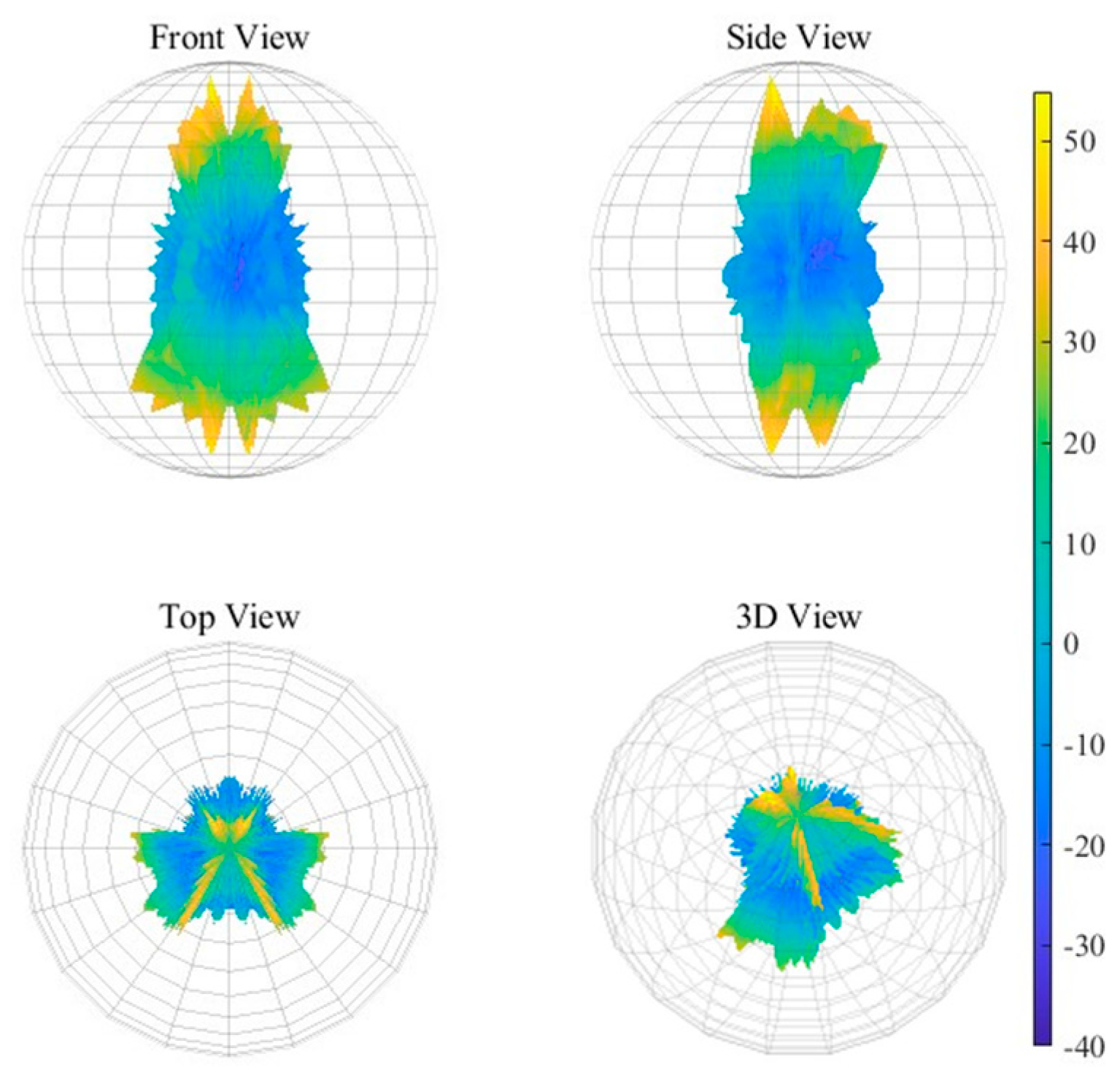
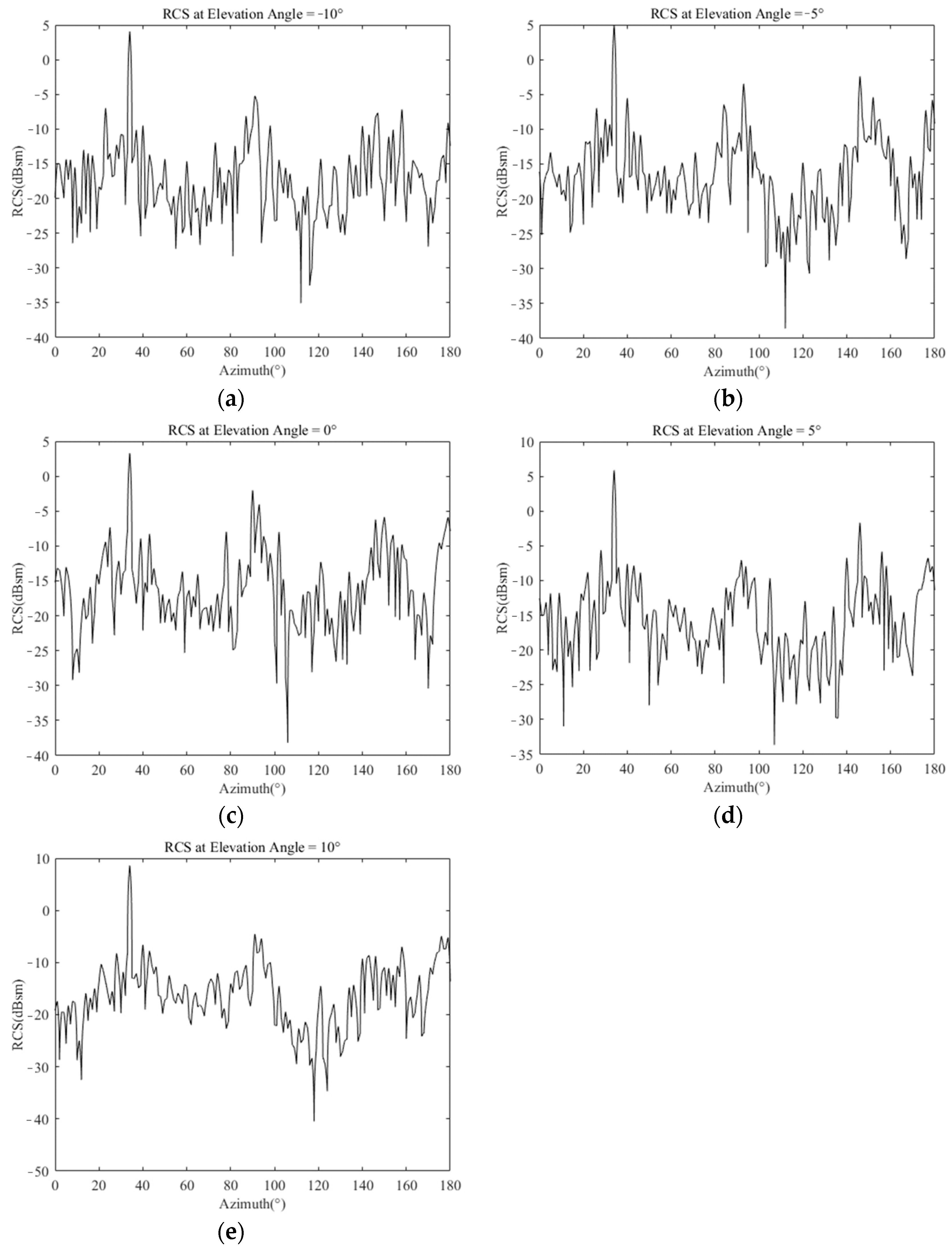
Three-dimensional RCS data of a typical flying wing stealth aircraft are presented in Figure 2 which were calculated using FEKO 2022.3 version software. Details of the RCS at elevation angles of −10, −5, 0, 5, 10 degrees are shown in Figure 3 as examples.
The unit for the RCS values in Figure 3 is d B s m , and the relationship between d B s m and m 2 is shown in Equation (3).
R C S d B s m = 10 × l o g 10 R C S ( m 2 )
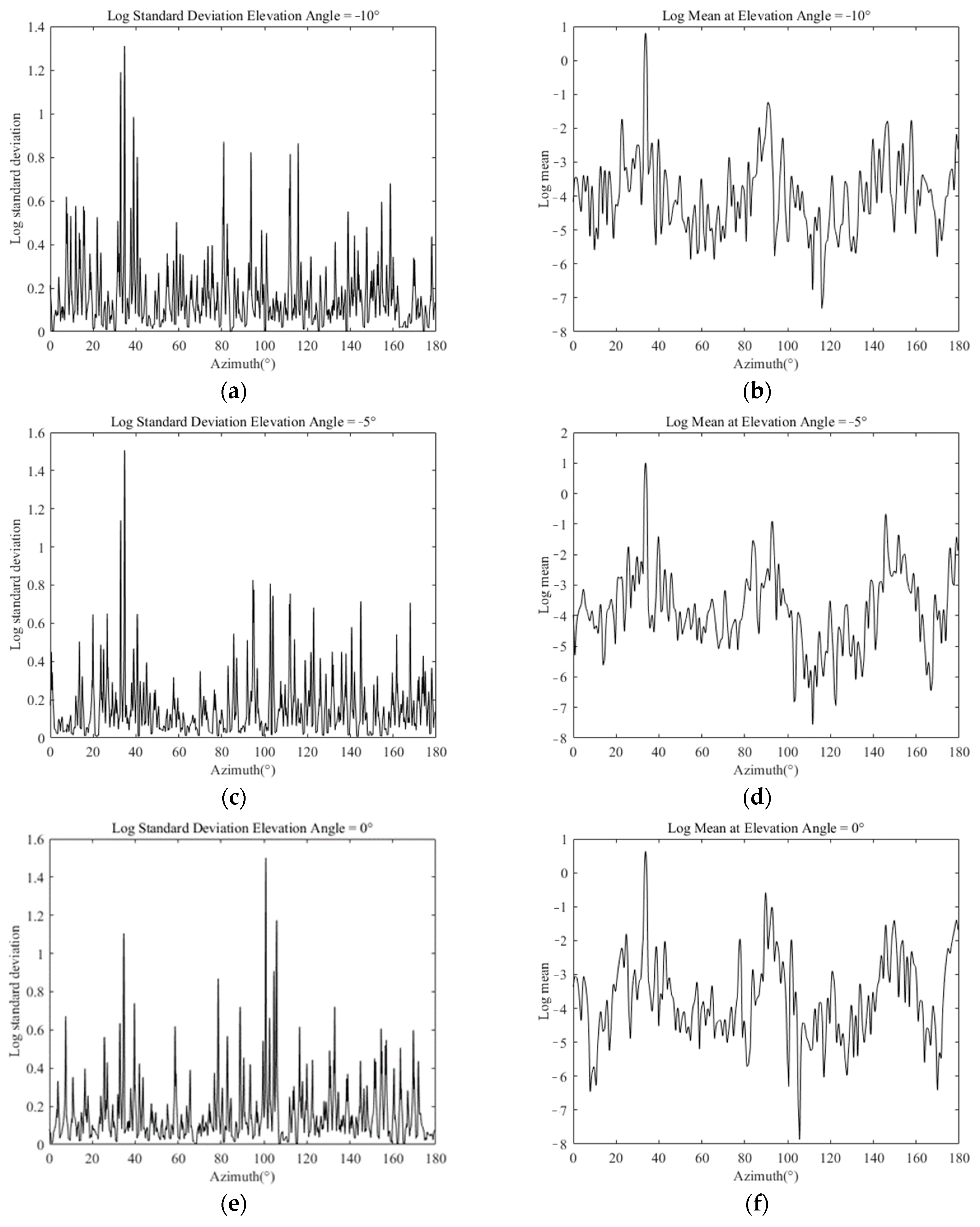
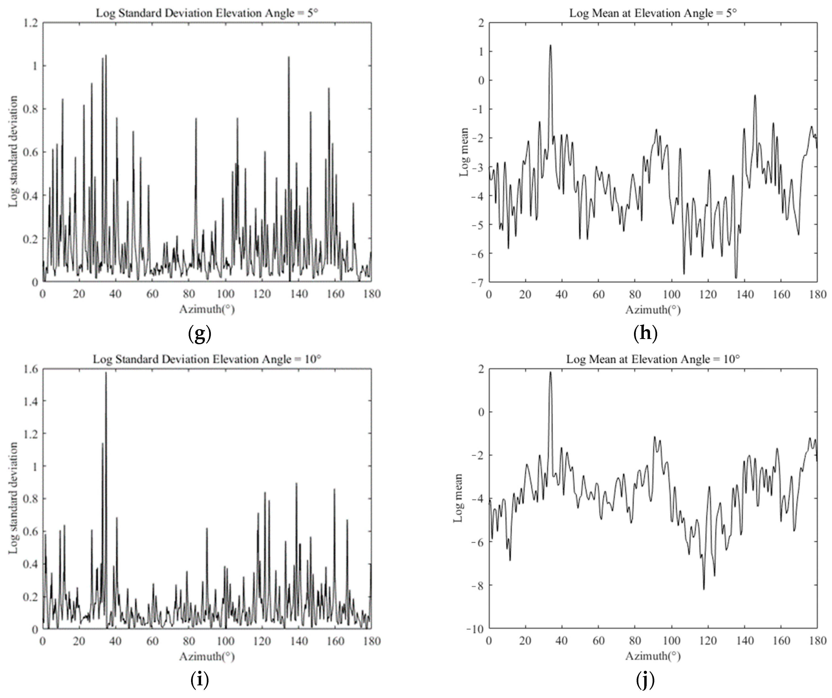
As shown in Figure 3, when the elevation angle is within the range of −10° to 10°, the peak RCS values occur at azimuths of 34 ° , 90 ° and 146 ° , which are called danger azimuths. Based on the RCS data, the parameters S d and σ m are fitted in log-normal distribution for every 0.5 ° with the RCS in m 2 in an all-angle domain. The results of the azimuth-varying log standard and log mean at elevation angles of −10°, −5°, 0°, 5°, 10° are shown in Figure 4 as examples.
With the azimuth-varying log standard and log mean, the RCS dynamic fluctuation statistical model could be obtained according to the elevation and azimuth angles at the waypoint.

2.2. Flight Parameters and Radar Relative Angle Calculation

To complete the detection probability calculation during penetration, it is necessary to obtain the radar relative angle and distance, the fuel consumption, the attitude of the aircraft and the engine thrust at every moment.

2.2.1. Solving Flight Parameters

Trajectory is defined by several points with speed and position, so acceleration can be solved using the difference method. Since the difference method will lead to the loss of the initial point, the acceleration and speed are both taken as the value of the second point.
Based on the acceleration, a kinetic equation is set up in the wind coordinate frame, which means that the forces on the aircraft should be converted to the wind coordinate frame by a transform matrix. The coordinate frames involved in the process of the flight parameter calculation are the wind coordinate frame, body coordinate frame and track coordinate frame. A transition matrix L a b converting from body to wind coordinate frames can be expressed as
L ab = cos α cos β sin β sin α cos β cos α sin β cos β sin α sin β sin α 0 cos α
where the parameter α is the angle of attack and β is the angle of sideslip. It is assumed that β = 0 , which means only the forces in the symmetrical plane are considered. Ignoring the engine angle, the thrust in the wind coordinate frame can be expressed as
F T a = L ab T 0 0
The transform matrix from the ground to the track coordinate frame is
L k g = cos θ a cos ψ a cos θ a sin ψ a sin θ a sin ψ a cos ψ a 0 sin θ a cos ψ a sin θ a sin ψ a cos θ a
where ψ a is the course angle of the aircraft and θ a is the climb angle.
The transform matrix from the track to the wind coordinate frame is
L a k = 1 0 0 0 cos ϕ a sin ϕ a 0 sin ϕ a cos ϕ a
The parameter ϕ a is the angle between the symmetrical plane of the aircraft and the plumb plane containing the velocity vector. Then, the gravity in the wind coordinate frame is
F G a = L ak L k g m 0 0 g
The aerodynamic forces can be expressed as
F A a = 1 2 ρ V 2 S C D α 0 C L α
As mentioned in Section 2.1.1, the lift coefficient C L and drag coefficient C D are functions of the angle of attack, which is obtained by interpolation according to the Mach number. In this case, the dynamic equation in the wind coordinate frame can be shown by
L ak L k g m a x a y a z + F G a + F T a + F A a = 0
Considering that the angle of attack is small, the trigonometry can be simplified as follows:
cos α = 1 ,     sin α = α
By solving the equation, the values of α , ϕ a and T are obtained, which means the transform matrix is fully defined.

2.2.2. Radar Relative Azimuth and Elevation Angle Calculations

Given the aircraft’s position x   y   z a and the radar system’s position x   y   z r in the ground coordinate frame, the radar’s relative displacement vector is
s g = x r x a y r y a z r z a
As mentioned above, the parameters of the RCS dynamic fluctuation statistical model are related to the radar relative azimuth angle. So, the displacement vector needs to be projected into the body coordinate frame, which can be written as
s b = L ab T L ak L kg s g = s x b s y b s z b
Then the azimuth and elevation angles can be expressed as
ψ r = arccos s x b s x b 2 + s y b 2
θ r = arcsin s z b

2.3. Algorithm of Radar Detection Probability

The most widely used method in radar signal detection is threshold detection based on the Neyman–Pearson criterion [8]. Threshold detection means that if the output of the radar receiver exceeds the threshold voltage, it is considered that the target exists; otherwise, it does not. Hence, the detection probability is the integral from the threshold voltage to positive infinity, which can be written as
P D = V T p v v d v
The parameter P D represents the detection probability. v is the signal strength, consisting of N vectors of the signal superimposed with Gaussian noise. p v ( v ) is the probability density function (pdf) of the detection probability. And V T is the detection threshold obtained from the false alarm probability, which will be explained in detail below.
The Laplace transform of p v ( v ) is
L v s = 0 p v v e s v d v
Based on the formulas above, the algorithm of radar detection probability is established.

2.3.1. Algorithm of Radar Detection Probability in a Single Position

To describe the detection probability accurately, the probability density function and the correlation parameter ρ are required. The correlation parameter describes the correlation of the time-varying RCS between echo pulse sequences.
Referring to Kanter’s study [9], the method suitable for an exponentially correlated signal in Gaussian noise is chosen to calculate the radar detection probability. The correlation matrix is introduced as
C = 1 ρ ρ N 1 ρ 1 ρ N 2 ρ N 1 ρ N 2 1
where N is the coherent accumulation, that is, the number of pulse signals. The value of the matrix can be expressed as
C k n = ρ k n
where k and n are the numbers of rows and columns in the matrix. And the eigenvalue of the correlation matrix is λ i ,   i = 1 , , N .
As shown in Kanter’s study [9], the Laplace transform L v ( v ) can be represented by the equation below, which is related to the eigenvalues of the correlation matrix.
L v s = 1 1 N [ 1 + χ λ n s + 1 ]
where the parameter χ is the signal-to-noise ratio (SNR).
When ρ 1 , that is, when the eigenvalues are different, the pdf of the integrator output according to the inverse Laplace transform of Equation (20) can be expressed as
p v v = n = 1 N k = 1 k n N 1 1 + χ λ k 1 + χ λ n 1 e v 1 + χ λ n 1 + χ λ n
The threshold value V T can be calculated by specifying the false alarm probability P F A .
P F A = e V T n = 0 N 1 V T n n !
Then, as shown in Ref. [9], the detection probability P D can be written as
P D = n = 0 N k = 1 k n N 1 1 + χ λ k 1 + χ λ n 1 e V T 1 + χ λ n
Following the above steps shown in Kanter’s study [9], when ρ = 1 , the correlation matrix can be written as
C ( ρ = 1 ) = N 0 0 0 0 0 0 0 0
Then, the Laplace transform under the condition ρ = 1 can be represented as
L v s = 1 1 + χ N s + 1 s + 1 N 1
So, the derivation result of the detection probability formula is as follows:
P D = N χ + 1 N 1 N χ N 1 e V T N χ + 1 k = 0 N 2 N χ + 1 N 2 k k ! N χ N 1 k · e V T i = 0 k C k i V T k i  

2.3.2. Algorithm of Radar Detection Probability of the Entire Trajectory

According to the radar equation, the relationship between the SNR, RCS and the relative distance can be expressed as
χ σ , R = K σ R 4
where R is the relative distance, and the parameter K is defined by the specific radar.
Considering the RCS fluctuation, the detection probability can be expressed as follows with the RCS probability density function used for weight addition.
P D = 0 p σ n = 0 N k = 1 k n N 1 1 + χ σ , R λ k 1 + χ σ , R λ n 1 e x p ( V T 1 + χ σ , R λ n ) d σ
Note that the parameter R is time-varying.
Since there are multiple scans in the entire trajectory, the cumulative detection probability of the whole trajectory can be expressed as
P D r o u t e = 1 1 N 1 P D

2.4. Trajectory Planning Based on Sparse A* Algorithm

The A* algorithm was originally proposed by Hart [15]. As a typical trajectory-planning algorithm, it has been widely used for its stability, simplicity and ease of implementation.
The sparse A* Search algorithm (SAS) is an improved A* algorithm [1]. According to the SAS, the space of the node search can be reduced considering constraints, which can improve the search efficiency of the algorithm. In this paper, a sparse A* algorithm to extend waypoints using a three-dimensional spherical grid is constructed, and a cost function related to the flight distance and detection probability is defined.

2.4.1. The Steps of the Sparse A* Algorithm

The steps of the sparse A* algorithm are given as follows, named Algorithm 1.
Algorithm 1. The sparse A* algorithm
Input: Coordinates of the start node P s , coordinates of the goal node P g , weight, step size, grid properties, number of sectors S, radar layout.
Output: Trajectory.
1: Close Set = { P s };//Initialization
2: Open Set = {};//Initialization
3: Min Heap = { P s };//Initialization
4: Current Node = P s ;//Initialization
5: while ( D i s t a n c e C u r r e n t   N o d e ,   P g S t e p   s i z e ) do
6:      Open Set = {Generated nodes} according to Figure 5;
7:      Remove the nodes in Min Heap from Open Set;
8:      Calculate the cost according to Equation (30);
9:      Min Nodes = nodes with least cost in each sector;
10:    Min Heap append the Min Nodes;
11:    Best node = node with least cost in Min Heap;
12:    Current Node = Best node;//Update the Current Node
13:    Close Set append the Current Node;//Update the Close Set
14:    Open Set = {}
15:    Record the parameters;
16:    if ( S t e p   n u m b e r M a x   s t e p   n u m b e r ) then
17:           continue;
18:    else if
19:           break and exit.
20:    if (Min Heap is empty) then
21:           break and exit.
20: end while
21: Finish the calculation of the last step to the goal;
21: Trace back the Close Set to get the Trajectory;
22: return Trajectory
Firstly, the close set and current point are initialized according to the input start and goal, and the open set is extended from the current point using a three-dimensional spherical grid. The nodes with minimum cost in each sector are added to the min heap. Then, the point in the min heap with the lowest cost will be regarded as the best point. When the cycle times are less than the maximum step number, the best point is chosen as the next until the goal is achieved. In subsequent calculations, the number of sector divisions for the sparse A* algorithm is set to 3.

2.4.2. Node-Generation Method

The grid properties are defined to include R (step size), N (number of nodes), θ u (upward angle), θ d (downward angle) and θ l (lateral angle). For N = 9 , with the current node P 2 and the previous node P 1 , the expansion mode of the sparse A* algorithm is depicted in Figure 5.
As shown in Figure 5, the orange arrow not only represents the central shaft of the grid but also indicates the process of generating the central grid node. The blue dashed line is the spherical grid. The direction of the center shaft depends on the direction of the previous step, which was from P 1 to P 2 . For the first step, the direction of the center shaft is the direction from the start to the goal. The orange and black arrows indicate the process of grid generation by stepping from the current node.
To avoid unnecessary node expansion, the node is generated under certain constraints, including the flight altitude limitation and the maximum climb/descent angle, which are used to check whether the node is qualified. And the node will be corrected if it is outside the limits. In the simulations in the next section, the step size is set to 3 km, which is a small maneuver for a stealth aircraft when θ l = 8 ° ,   θ u = 0.5 ° and θ d = 0.5 ° .

2.4.3. Cost Function Definition

In the process of the trajectory planning, the cost function needs to be defined to evaluate the quality of the waypoint. Suppose that the set of waypoints is { p 0 ,   p 1 , ,   p n } when searching from the start node p 0 to node p n . The goal node is represented by p e . The total cost function of the current node p n can be expressed as
C o s t p n = k 1 L p 0 ,   p n + k 2 D p n , p e + k 3 P p 0 ,   p n + k 4 H ( p n 1 , p n ) + k 5 P ( p n )
where the function D ( p n , p e ) describes the linear distance between p n and p e , and the function L p 0 ,   p n is the total distance of the previous n moves, which can be expressed as
L p 0 ,   p n = i = 0 i = n 1 D ( p , p i + 1 )
The expression P ( p 0 , p n ) in the cost function is the radar cumulative detection probability of the trajectory composed of { p 0 , p 1 , , p n } . The expression H ( p n 1 , p n ) represents the height difference between p n and p n 1 . The expression P ( p n ) represents the radar single detection probability at the current node p n , and the parameters k 1 , k 2 , k 3 , k 4 and k 5 are the weights of each cost.
In this case, the next node can be selected by weighing the cost of the distance and the cost of the radar detection probability.

3. Results

The diversity of radar threat scenarios necessitates that trajectory selection be contingent not only on the arrangement of radars but also on their power factors. To thoroughly evaluate and analyze the 3D-SASLRM method, simulations are executed in three scenarios, each under three different levels of radar power.
Referring to airborne radars, standard ground-based radars and military ground-based radars, the chosen radar powers are 5 × 10 5 , 1 × 10 4 and 3.9063 × 10 3 , respectively. These are categorized as low-power, medium-power, and high-power radars in the subsequent discussion. And the radar parameters for these three categories are delineated in Table 1.
The single valley radius of a radar system is defined as the radar distance at which the radar single detection probability reaches 30% when approaching the radar at an RCS of −20 d B . This implies that it is impossible for an aircraft, even with the small RCS value of −20 dB, to successfully penetrate the radar’s coverage once within its single valley radius. In the following analysis, the single valley radius is referred to as the SVR for short.
Subsequently, simulations are executed in three different scenarios with different radar powers involving one, three and ten radars, respectively. Since the straight-line trajectory has the lowest distance cost, it is used for a comparative analysis against the trajectory planned afterwards.

3.1. Stealth Aircraft Penetration in a Single-Radar Threat Environment

3.1.1. Conditions

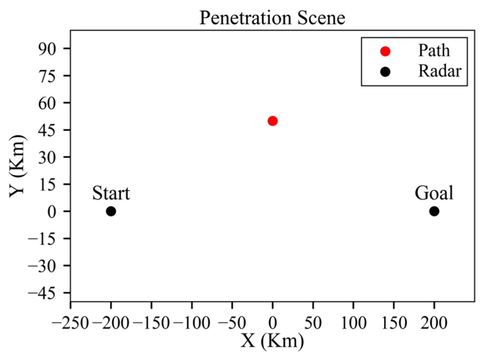
As shown in Figure 6, the mission is defined as penetration from (−200, 0, 8) to (200, 0, 10).
For the threat environment, the radar performance parameters are set as follows.
In Table 2, T s c a n is the radar scan period, P F A is the false alarm probability, N is the number of pulses, ρ is the correlation parameter, V H is the hover speed and R H is the hover radius. As shown in Table 2, there is a fixed radar located in (0, 50, 0) in the threat environment.
For the sparse A* Algorithm, the parameters are given in Table 3.
The “Number of Expanded Nodes” means the number of generated nodes when stepping from the current node to the next node. The weight parameters k 1 ,   k 2 and k 3 are used for the calculation in Equation (30). With the parameters in Table 2 and Table 3, a trajectory with low radar detection probability can be found using the 3D-SASLRM method.

3.1.2. Results of the Straight-Line Trajectory

The trajectory in a straight line is identified as the trajectory established prior to planning. The results at varying levels of radar power are presented below.
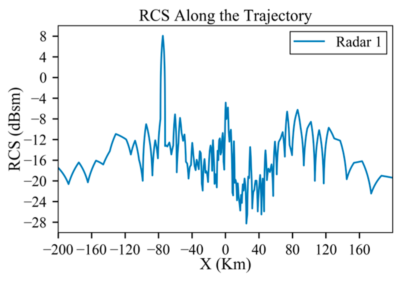
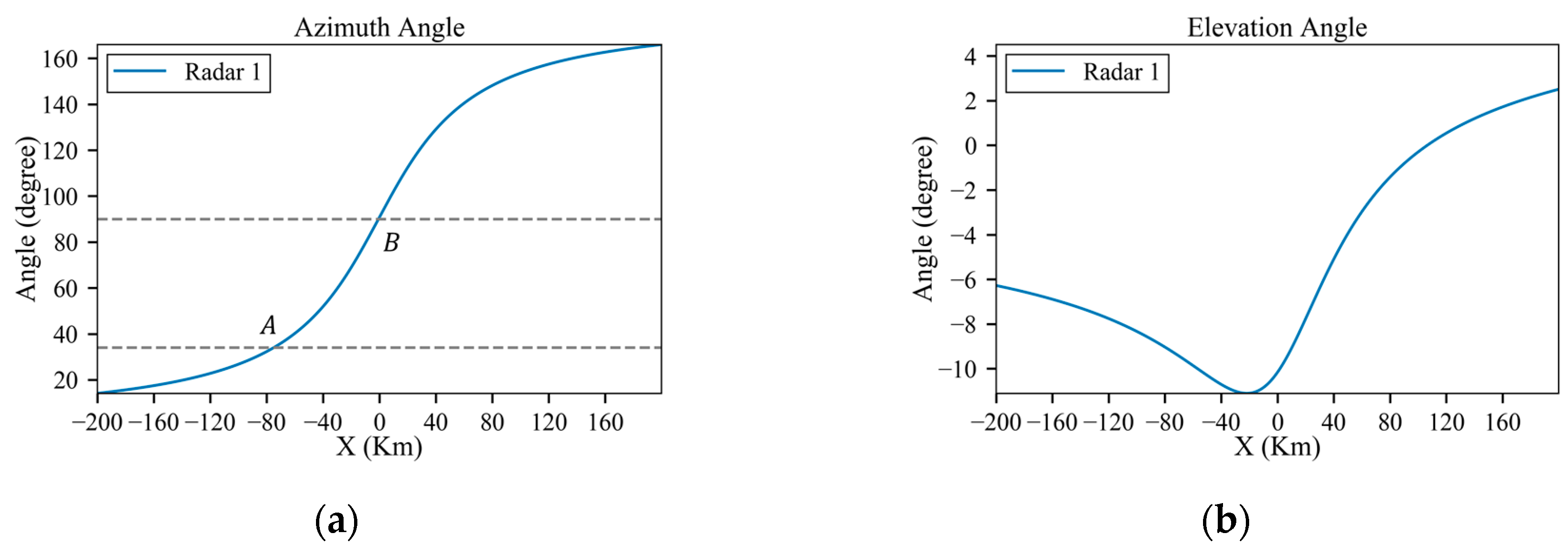
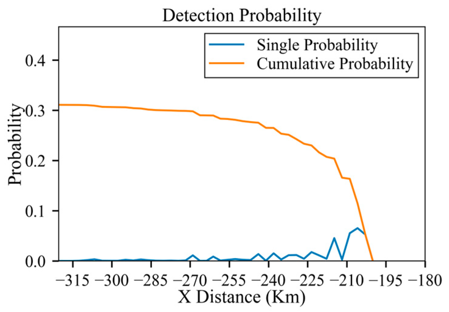
The term “Single probability” means the detection probability per radar scan period, whereas the “cumulative probability” is the detection probability of the whole trajectory. Figure 7 displays the original RCS data interpolated by the azimuth angle in Figure 8a. So, the RCS values in Figure 7 are independent of the radar distance. Figure 8b indicates the variation in the elevation angle throughout the trajectory. An analysis of the original RCS data reveals that the peak exposure angles of the aircraft are 34 ° , 90 ° and 146 ° , which may significantly increase the detection probability. Corresponding to Figure 8a, the peak exposure positions are located at X = 74.13   k m , X = 0   k m and X = 75   k m . Since the radar distance at X = 75   k m is considerable and the peak is weaker, the influence on detection probability mainly comes from X = 74.13   k m and X = 0   k m , denoted as A and B, respectively. Figure 9 shows the detection probability for different radar powers, which indicates that the detection probability rapidly grows as the radar power increases. Under low-power, medium-power and high-power radars, the probabilities of detection are 43.2%, 88.2% and 100%, respectively. And the peaks of the single probability in Figure 9 coincide with positions A and B in Figure 8a.

3.1.3. Results of the Planned Trajectory

Considering the distance cost and the detection probability cost, the results of the trajectory planning using the 3D-SASLRM method are shown below.
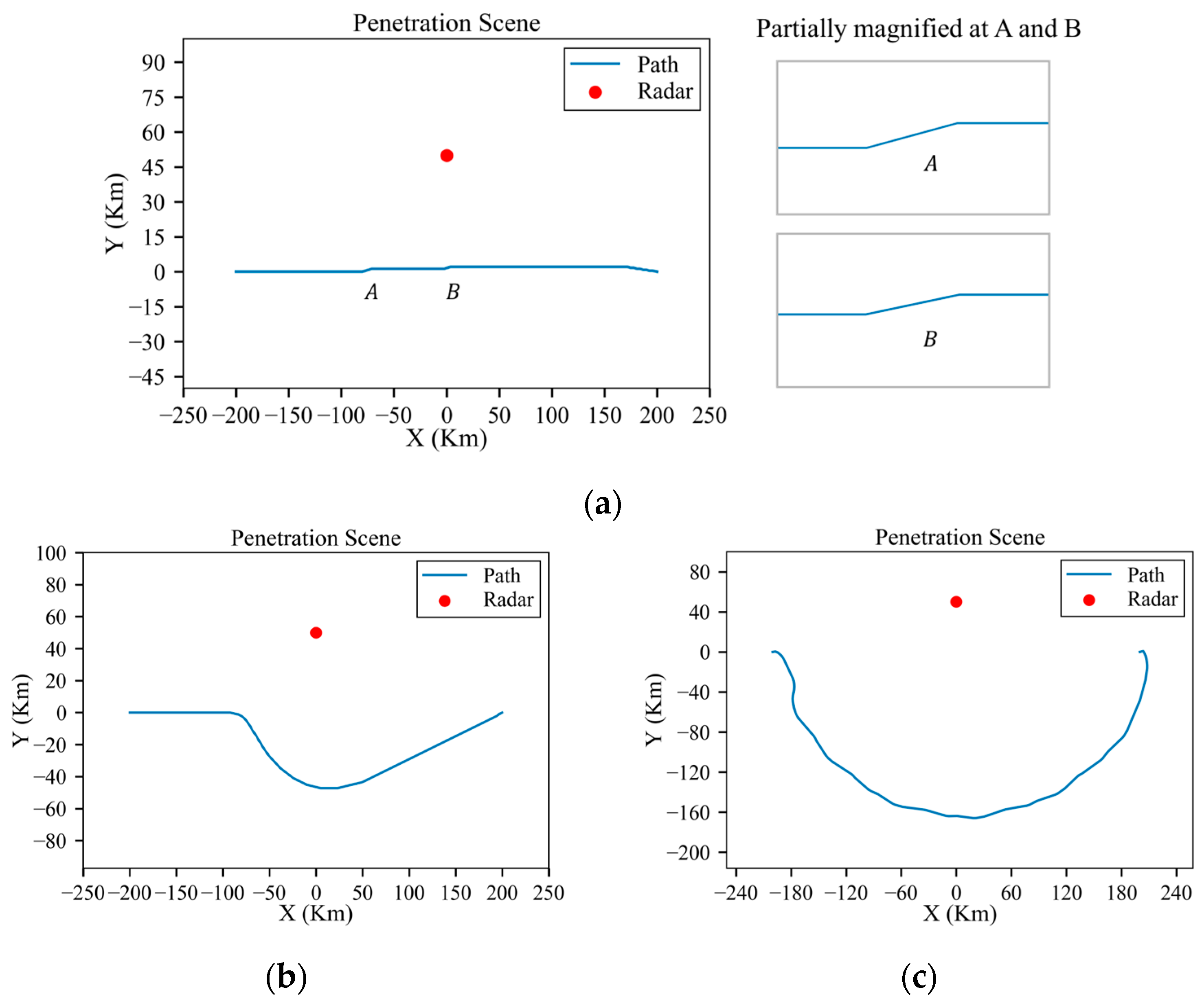
According to the results of the straight-line trajectory, the danger positions A and B are marked and partially magnified in Figure 10a. Figure 11 displays altitude variations during flight, ranging from 8 km at the start to 10 km at the goal. It is evident that the higher the radar’s power, the faster the climb rate of the aircraft. This is because when the radar power is high, the trajectory planning is dominated by survival, so the aircraft will fly away from the radar as quickly as possible, while with lower-power radar, the trajectory planning balances both survivability and economy. Figure 12a and Figure 13a indicate variations in the azimuth and elevation angles along the planned trajectory under the low-power radar, which show sudden changes at the danger positions A and B. As shown in Figure 10a, the trajectory deflects at these danger positions, suggesting that the aircraft needs to execute maneuvering turns to avoid the RCS peak exposure. This finding is consistent with Lu’s study [16]. And Figure 14 displays the detection probability in each environment.
As observed in Figure 10a, the planned trajectory under low-power radar only requires minor maneuvers at the danger positions A and B to avoid RCS peaks. And under medium-power and high-power radars, the aircraft needs to perform large-radius maneuvers in advance to reach the destination, aiming to maintain a safe distance from the radar.
According to Figure 14, a comparison of detection probabilities before and after planning under different radar power settings is presented in Table 4.
Based on the above analysis, it is concluded that minor maneuvers can significantly reduce the probability of detection while also saving distance in the case of low-power radars. And under medium-power and high-power radars, more flight distance is necessitated to maintain a safe separation from the radar.

3.2. Stealth Aircraft Penetration in Three-Radar Threat Environments

Based on the analysis of Section 3.1, simulations in three-radar scenarios are constructed.

3.2.1. Conditions

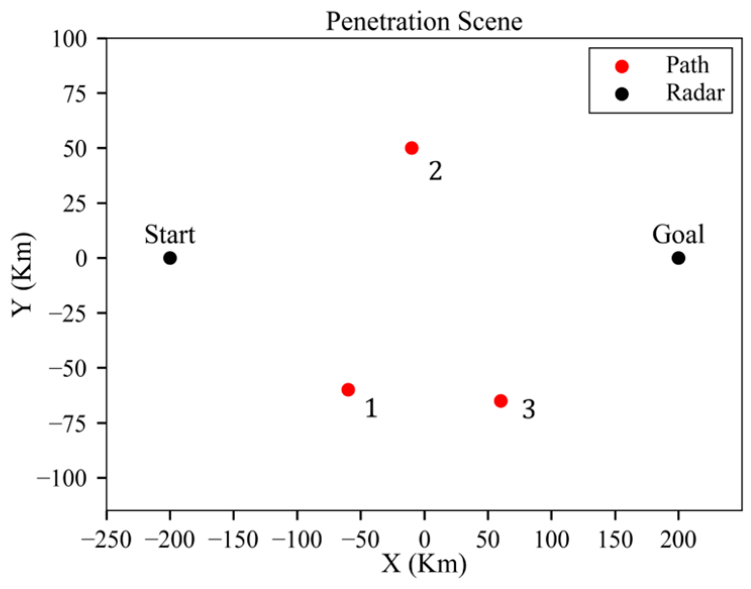
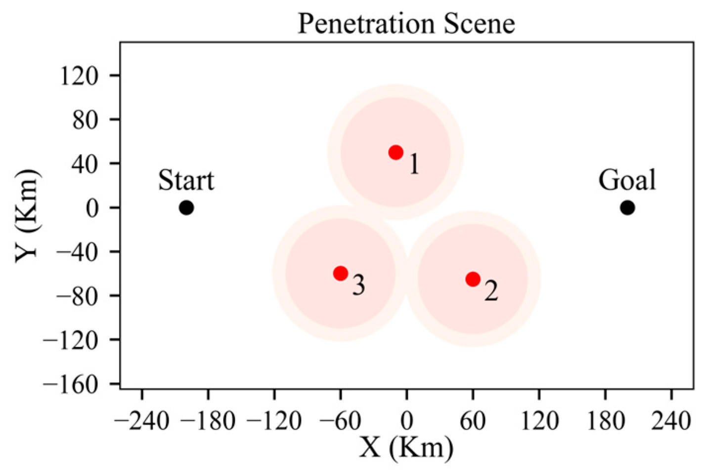
As shown in Figure 15, the mission is defined as penetration from (−200, 0, 8) to (200, 0, 8).
For the threat environment, the radar performance parameters are shown in Table 5.
For the sparse A* Algorithm, the parameters are given in Table 6.
Based on the parameters in Table 5 and Table 6, a trajectory with low radar detection probability can be found using the 3D-SASLRM method.

3.2.2. Results of the Straight-Line Trajectory

Similar to Section 3.1, a straight-line trajectory is defined for comparison to validate the effectiveness of the algorithm. The calculation results are as follows.
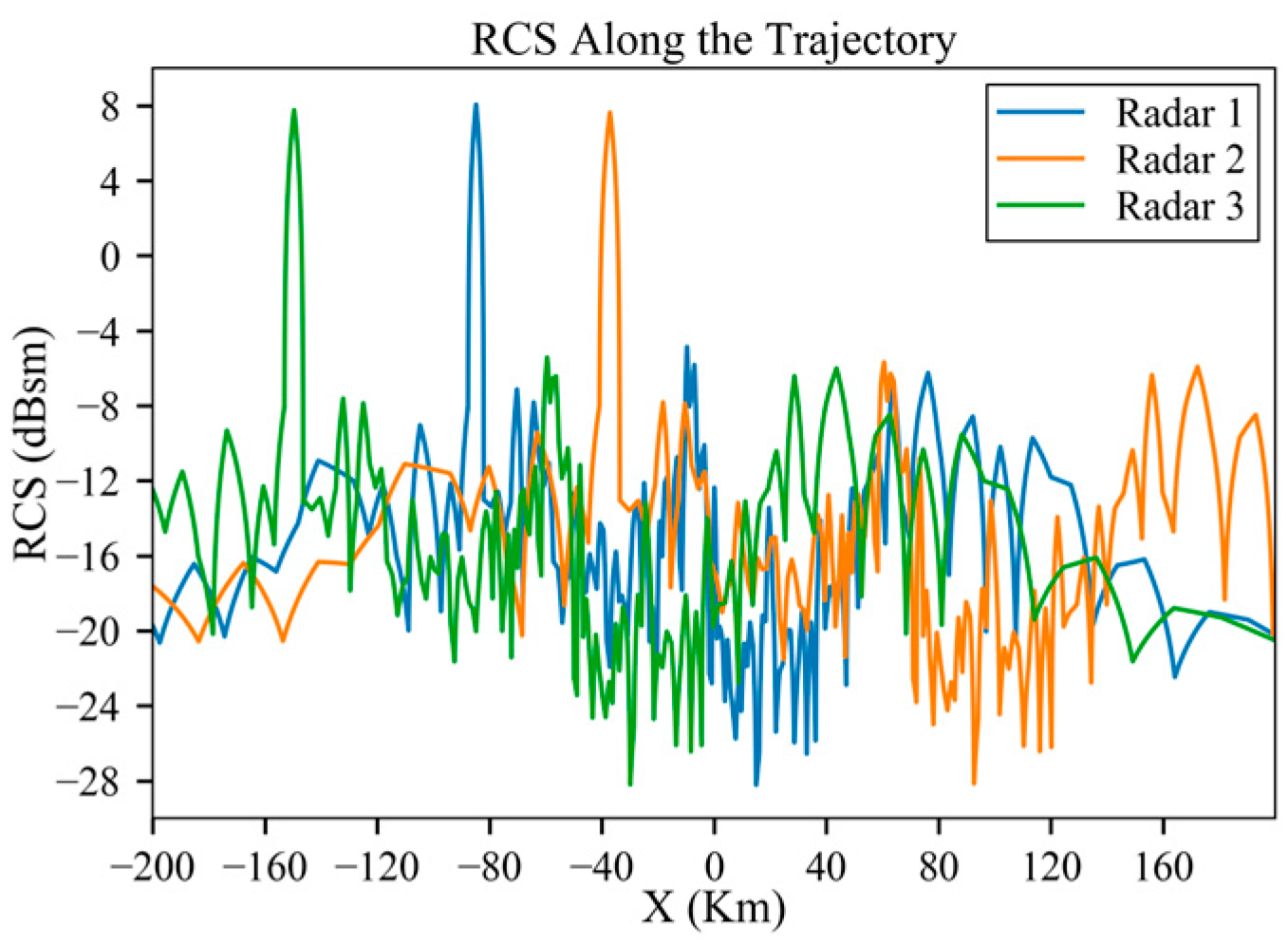
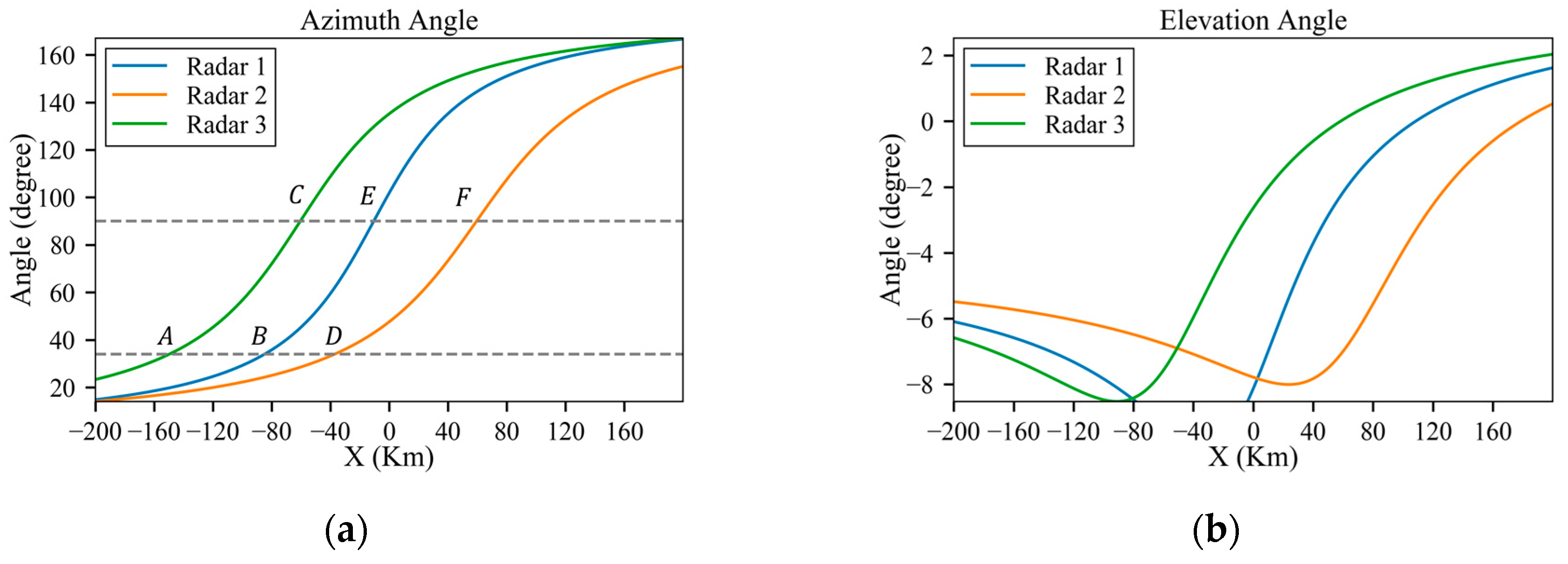
Similar to Section 3.1, due to the radar distance, the influence of the third peak 146 ° on the detection probability is not considerable. Figure 16 displays the original RCS data, interpolated based on the azimuth angle, as shown in Figure 17a. According to the azimuth angle along the trajectory in Figure 17a, the aircraft experiences three instances each of peak exposure at 34 ° and 90°. These six peak positions are marked in Figure 18a,b. Due to the influence of radar power, the positions at which the detection probability obviously increases are A, B and E for low-power radars and the increases at C, D and F are weak, as shown in Figure 18a.
According to Figure 18, the final cumulative probabilities under low-power, medium-power and high-power radars are 42%, 91.7% and 100%, respectively.

3.2.3. Results of the Planned Trajectory

In the same scenario, the results obtained using the 3D-SASLRM method are as follows.
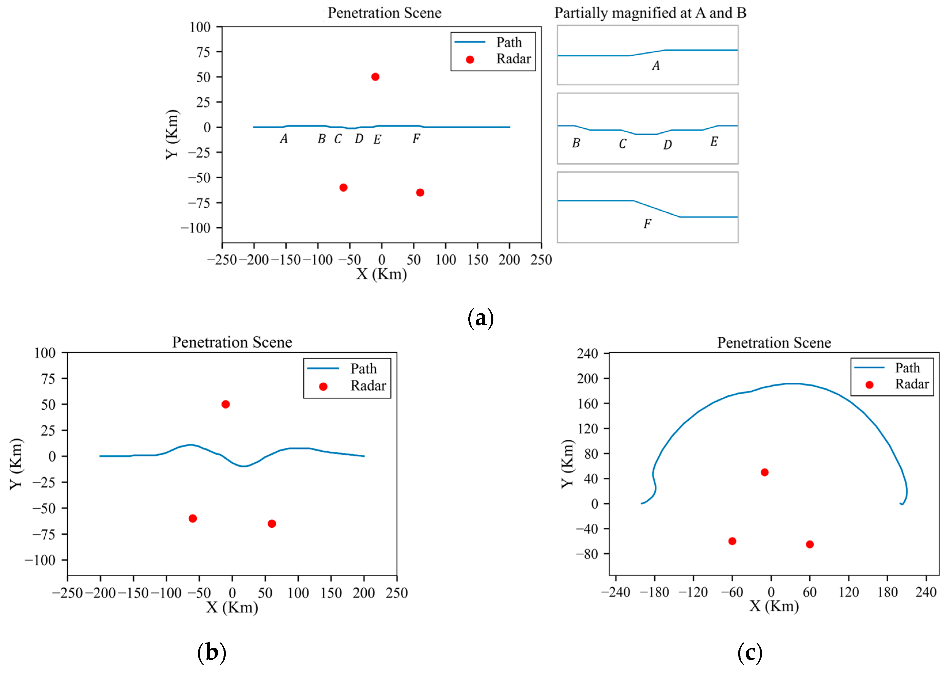
As shown in Figure 19a, Figure 20a, Figure 21a, Figure 22a and Figure 23a, the detection probability with low-power radars is significantly reduced by executing small maneuvers approximately at the danger positions. And for the scenarios involving medium-power and high-power radars, as shown in Figure 19b,c, Figure 20b,c, Figure 21b,c, Figure 22b,c and Figure 23b,c, the method involves increasing the flight distance to reduce the probability of detection. Since the starting and goal are at the same altitude, the aircraft can successfully penetrate without changing flight height, just as Figure 20 shows. And Figure 23 shows the detection probability in each environment.
Using the SVR to assess the threat level of radar is a method based on the consideration of the characteristics of both the radar and the aircraft. From the perspective of trajectory planning, it is necessary to introduce the concept of the cumulative valley radius (CVR).
The CVR of radar is defined as the radar distance at which the probability of radar cumulative detection reaches 30% when approaching the radar from 400 km away at an RCS of −20 d B . This implies that it is dangerous for an aircraft, even with a small RCS value of −20 d B , to approach a radar’s CVR from a long distance because of cumulative detection. In other words, in the context of a trajectory-planning scenario, approaching the CVR is already highly dangerous.
Given a high-power radar with an SVR of 50 km and a CVR of 62 km, the danger zone is shown in Figure 24. The light red area indicates the SVR, and the lighter-colored area surrounding it represents the CVR. It can be seen that passing through the radars to reach the destination is not feasible. In this case, a strategy of circumvention by moving around the sides is adopted.
According to Figure 23, a comparison of detection probabilities before and after planning for different radar powers is shown in Table 7.
Based on the above analysis, reasonable trajectories with low detection probabilities can be obtained for all three radar power levels.

3.3. Stealth Aircraft Penetration in Ten-Radar Threat Environment

In this section, a simulation of trajectory planning in a 3D complex multi-radar scenario is conducted. The radar systems include fixed radars and airborne early warning aircraft (AWACSs) on circular patrol routes.

3.3.1. Conditions

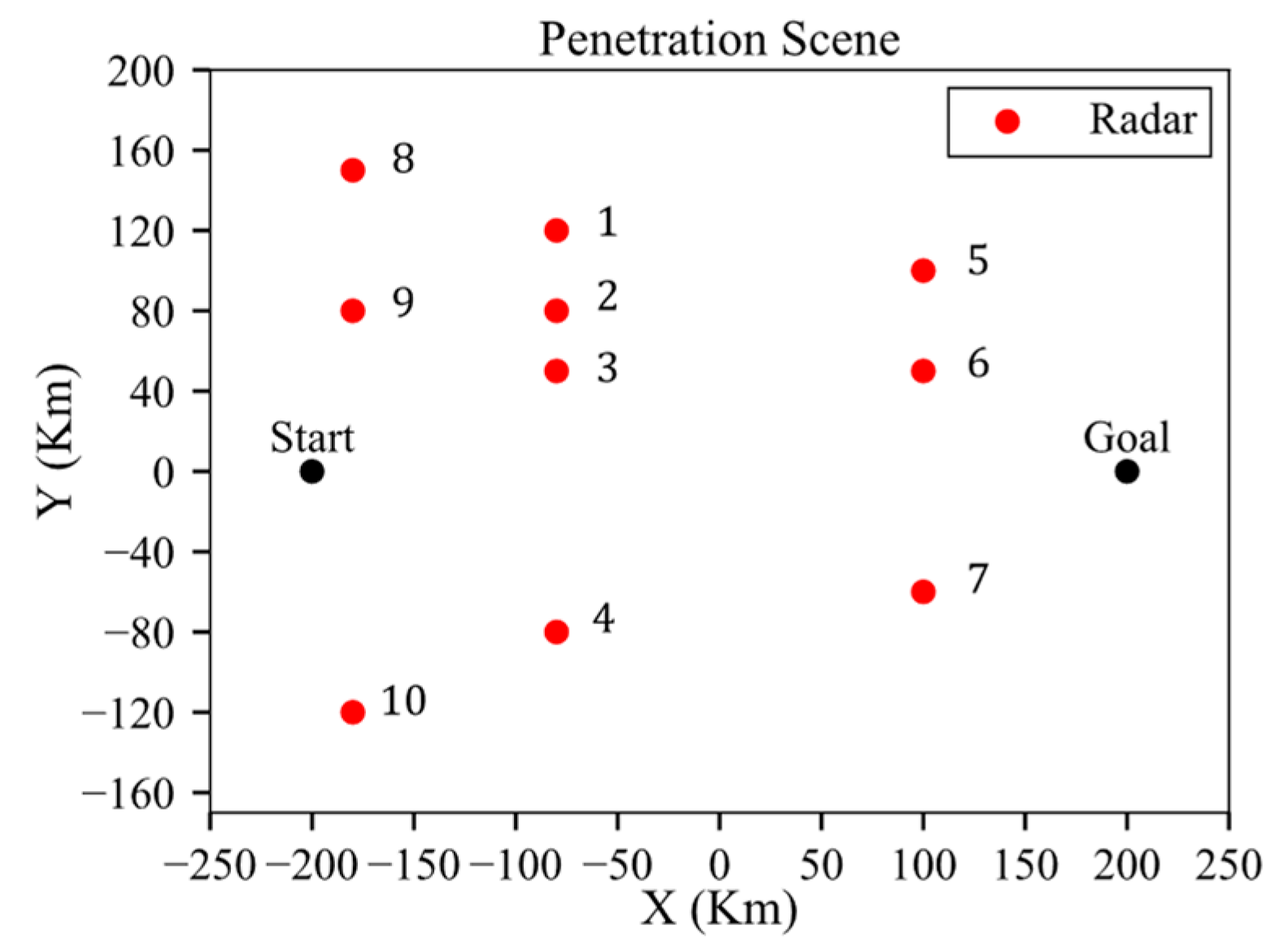
As shown in Figure 25, the mission is defined as penetration from (−200, 0, 8) to (200, 0, 8).
For the threat environment, the radar performance parameters are shown in Table 8.
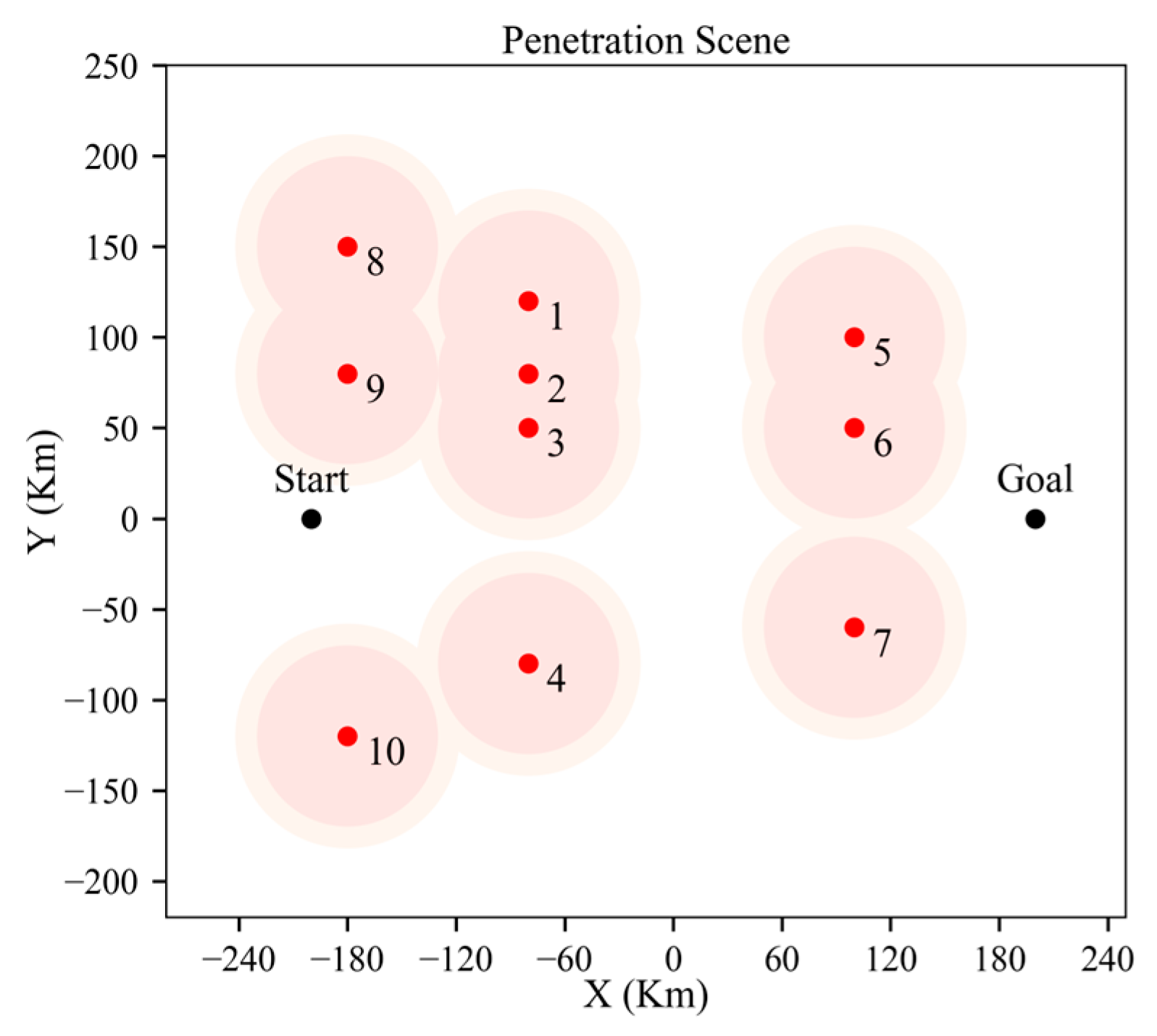
In the threat environment, numbers 1 to 7 represent fixed radars, and numbers 8 to 10 are AWACSs patrolling at an altitude of 10 km with a patrol radius of 10 km and a patrol speed of 200 m/s.
For the sparse A* Algorithm, the parameters are given in Table 9.
This research indicates that it is difficult to penetrate successfully under high-power radars due to their high power and tricky radar layout. So, the weight for high-power radars in Table 9 is denoted as “No solution”. Based on the parameters in Table 8 and Table 9, a trajectory with a low radar detection probability in an environment with low-power and medium-power radars can be found through the 3D-SASLRM method.

3.3.2. Results of the Straight-Line Trajectory

The calculation results of the straight-line trajectory are as follows.
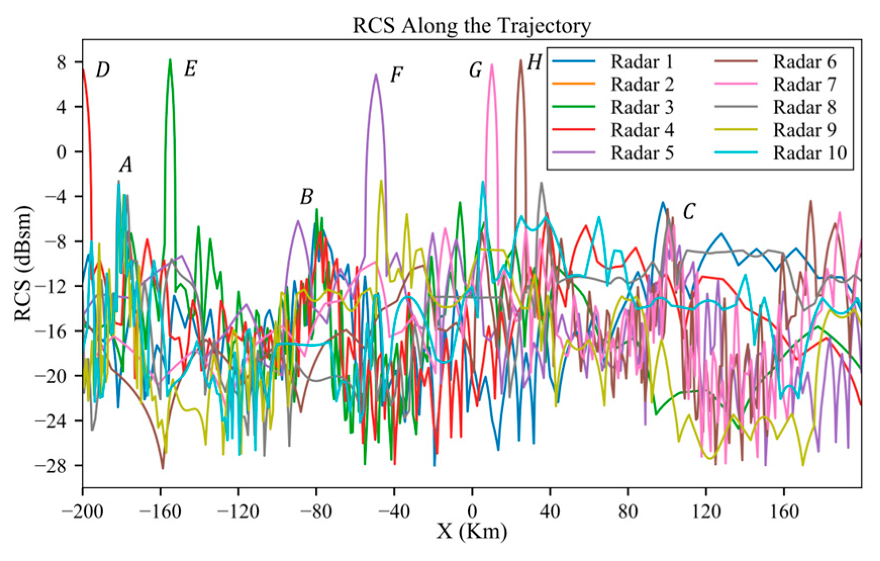
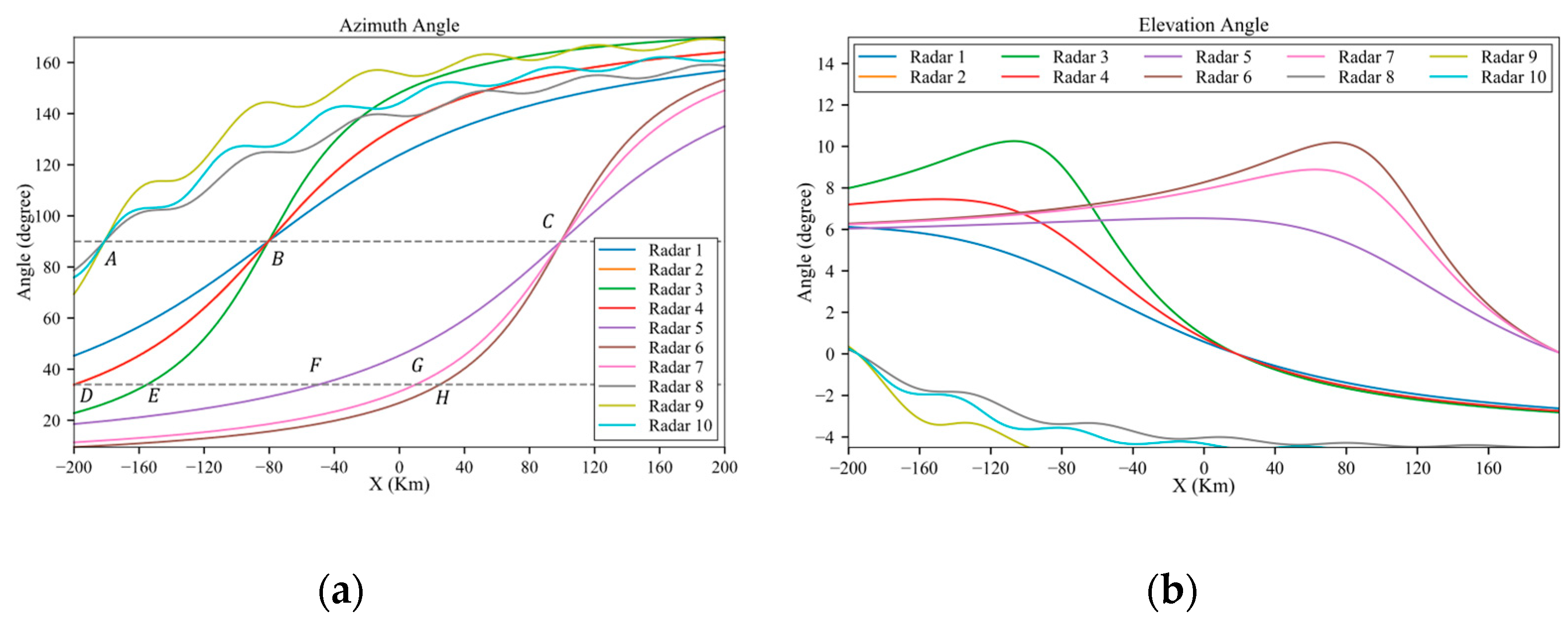
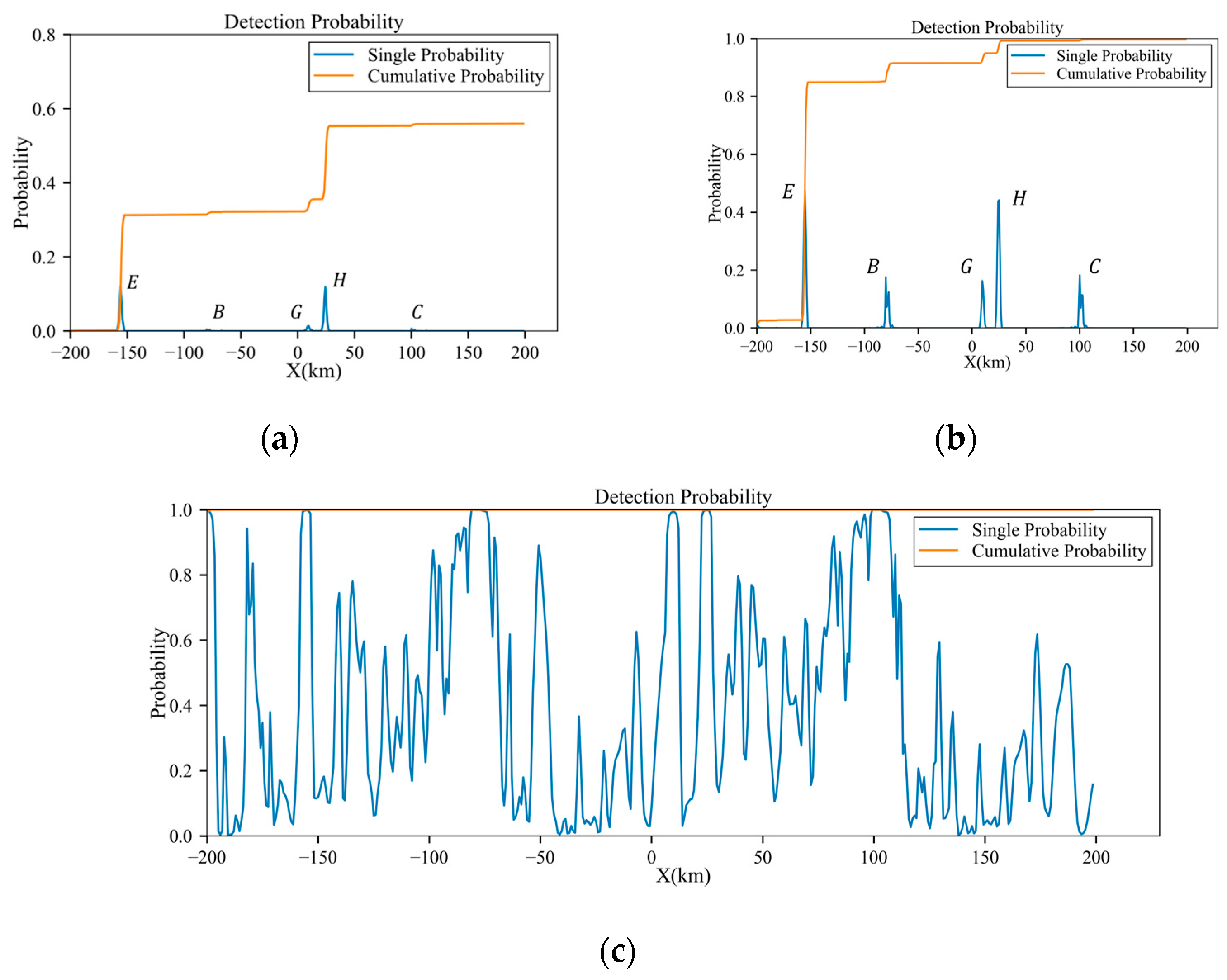
Similar to Section 3.1 and Section 3.2, the influence of the third peak 146 ° on the detection probability is not considerable. Figure 26 displays the original RCS data, interpolated based on the azimuth angle. As shown in Figure 27a, along the trajectory, the aircraft experiences five instances of peak exposure at 34 ° and three at 90°. Due to the influence of radar distance, the positions at which the detection probability sharply increases are only E, B, G, H and C, as shown in Figure 28 and the peaks under higher radar powers are sharper.
Figure 28 presents the final cumulative probabilities under low-power, medium-power and high-power radar conditions, which are 55.99%, 99.8% and 100%, respectively.

3.3.3. Results of the Planned Trajectory

In the same scenario, the results for environments with low-power and medium-power radars using the 3D-SASLRM method are as follows.
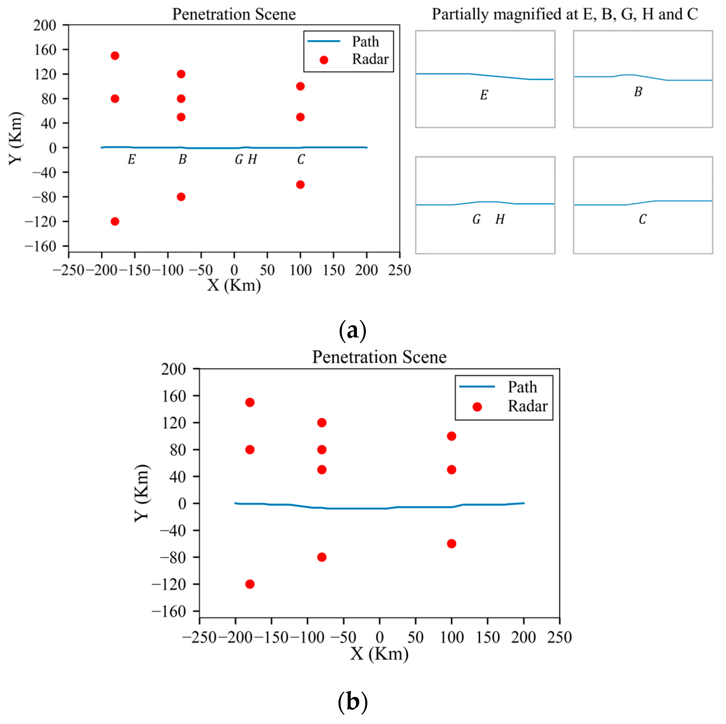
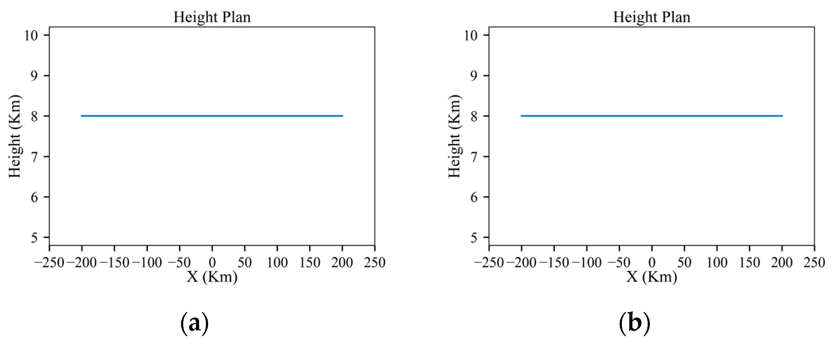
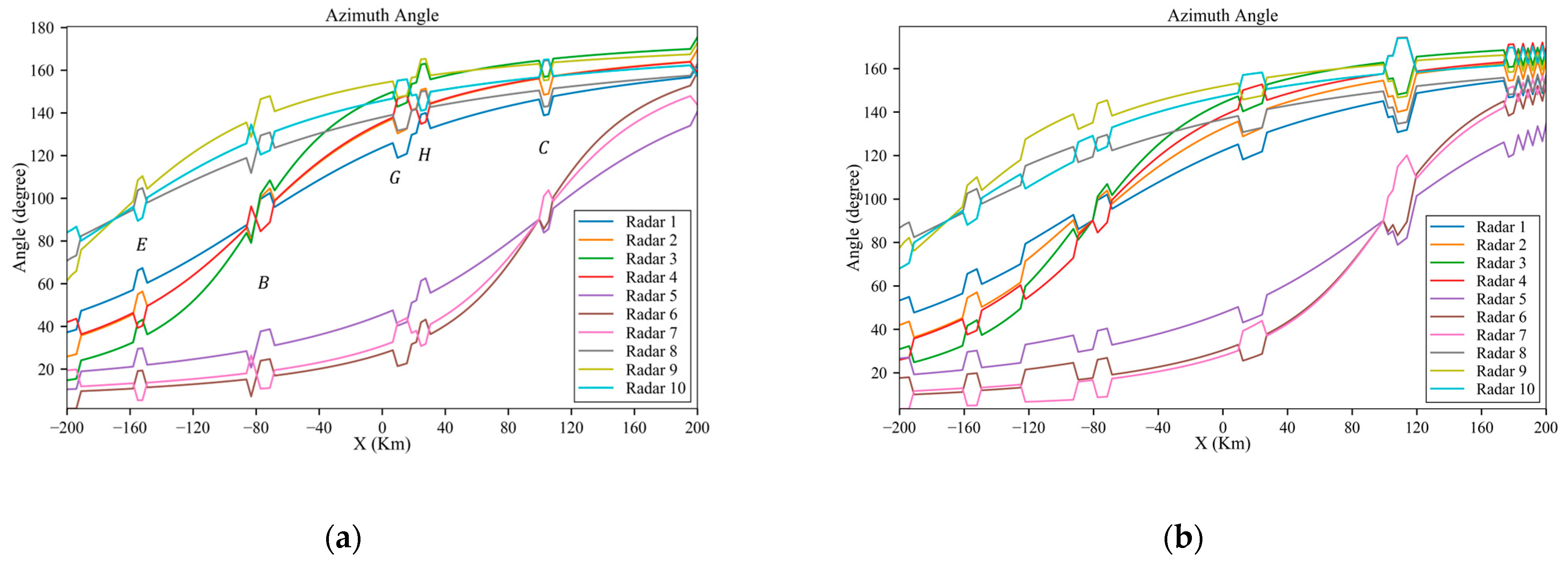
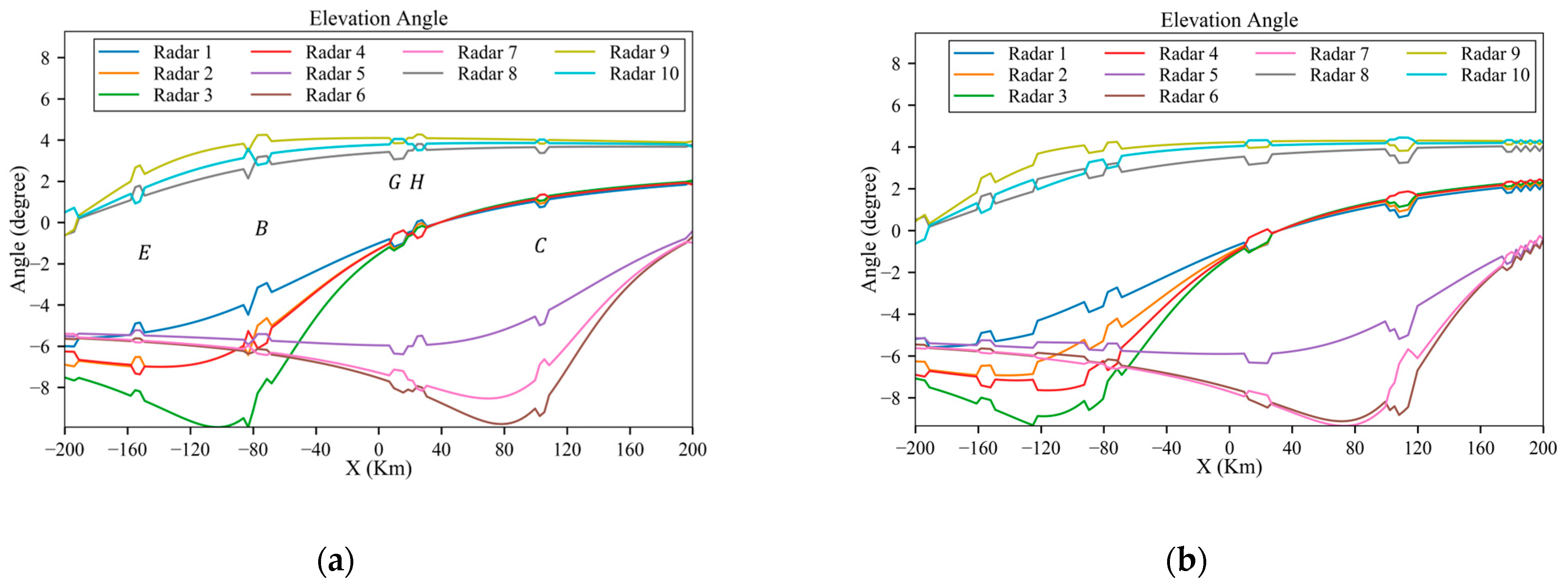
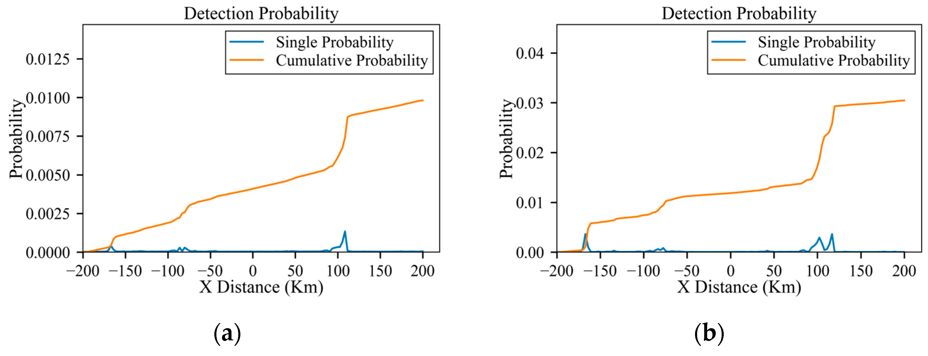
As shown in Figure 29a, in an environment with low-power radars, the aircraft can make appropriate maneuvers guided by the algorithm at danger positions E, B, G, H and C, which significantly reduces the radar detection probability. As shown in Figure 30, like the scenario in Section 3.2, the aircraft can penetrate without changing its altitude. Similarly, the azimuth and elevation angles along the planned trajectory are shown in Figure 31 and Figure 32, which show distinct changes at danger positions. Figure 33 presents the detection probability under low-power and medium-power radars.
Due to the high-power radar’s SVR being 50 km and the CVR being 62 km, a considerable part of the penetration area is occupied by the danger zone. As shown in Figure 34, the light red area indicates the SVR, and the lighter-colored area surrounding it represents the CVR.
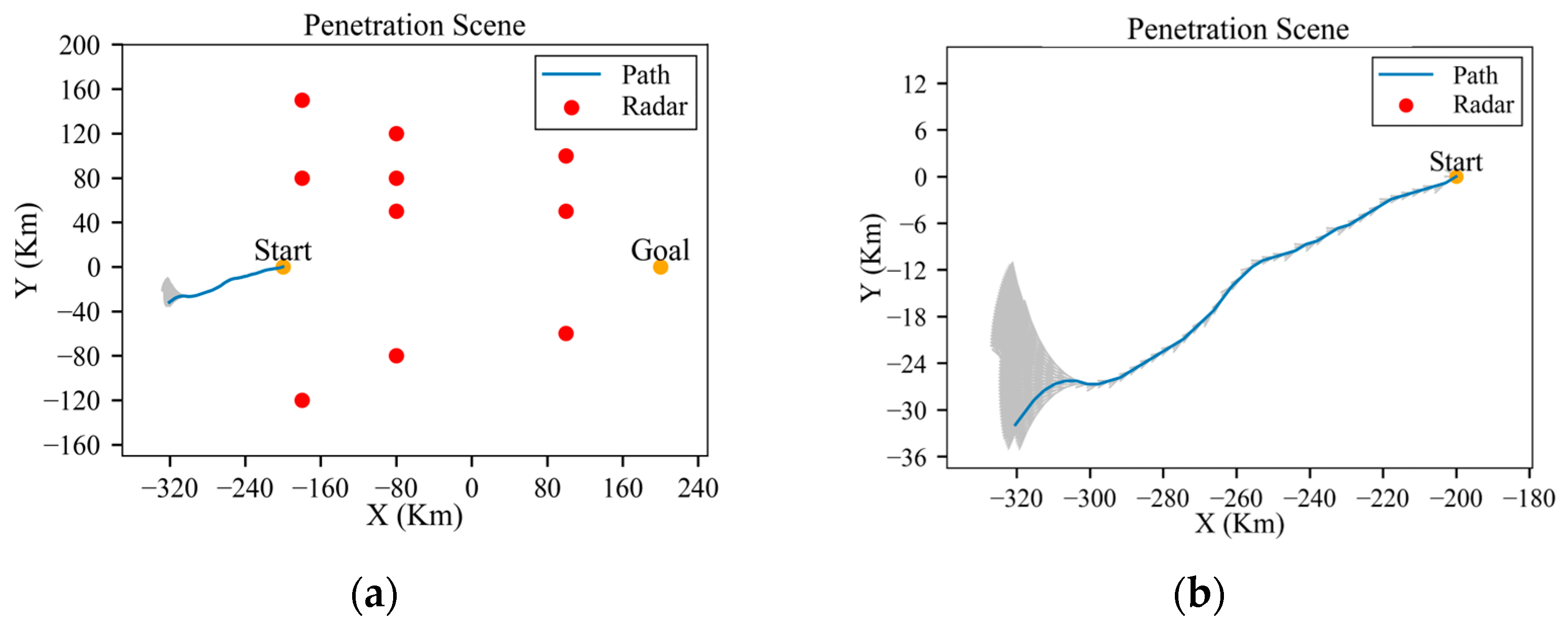
Therefore, within the penetration area, it is challenging to find a viable trajectory in the presence of so many radars and such a large danger zone. If the aircraft is allowed to head in the opposite direction as its first step, perhaps a trajectory with a low detection probability can be found. But even in this case, the cumulative probability of detection can escalate substantially, attributed to the large number of radars and their high power. In addition, this strategy results in a significant increase in flight distance cost. For example, Figure 35 depicts an attempt to circumvent the radars. The gray arrows in the figure represent the process of node generation by the SAS algorithm. However, as displayed in Figure 36, the cumulative probability of detection has already surged to 31% when the aircraft reaches the position shown in Figure 35.
A comparison of detection probabilities before and after planning in environments with low-power and medium-power radars is shown in Table 10.
Based on the above analysis, in environments with low-power and medium-power radars, a trajectory that significantly reduces the probability of detection can be found. And when there is a large number of high-power radars, it is difficult to find a trajectory within the penetration area.

3.4. Summary of the Simulation Results

A summary of the simulation results is presented in Table 11.
As shown in Table 11, the 3D-SASLRM method can provide reasonable trajectories in different scenarios. In a scenario with low-power radars, small maneuvers are adopted to avoid RCS peaks, while in scenarios with medium- and high-power radars, early large maneuvers are used to avoid approaching the radar valley radius. However, when there are many high-power radars, meaning the radar danger zone covers a very large area and even the detection probability at the start is considerable, it becomes difficult for the aircraft to penetrate successfully.

4. Conclusions

In this paper, a 3D sparse A* trajectory planning method based on a log-normal radar model (3D-SASLRM method) is constructed to enhance the survivability of penetration for stealth aircraft; this method which considers the RCS statistical uncertainty, the influence of the azimuth and elevation angles on the RCS and the statistical characteristics of the radar signal. An RCS dynamic fluctuation model is characterized by parameters including the log mean and log standard deviation, which vary with the radar relative azimuth and elevation angle. The method suitable for an exponentially correlated signal in Gaussian noise is chosen to calculate the radar detection probability as one of the costs of the sparse A* algorithm. By using 3D space simulations in complex adversarial scenarios, the following conclusions are obtained:
(1)
The 3D-SASLRM method established in this paper is effective at reducing the radar detection probability during penetration compared to the trajectory before planning.
(2)
For the RCS fluctuation model based on azimuth and elevation angles in 3D space, executing minor maneuvers at dangerous positions is an effective method in scenarios with low-power radars to reduce radar detection probability, which essentially decreases the time of high RCS exposure to radar.
(3)
In scenarios with medium-power and high-power radars, a trajectory with low detection probability can be found using early large maneuvers to avoid approaching the radar valley radius.
(4)
When the area enclosed by the radar valley radius almost covers the entire penetration area and the number of radars is large, it becomes difficult for the aircraft to reach the destination safely in the penetration area.
(5)
There are several aspects of the study that still need more in-depth research.
(a)
The computation time for the scenario in Section 3.3 is around 10 h, which should be decreased.
(b)
The weight of the sparse A* algorithm needs to be adjusted manually, which should be made more automated.
(c)
More work needs to be carried out on trajectory smoothing in 3D space.

Author Contributions

Conceptualization, X.L.; methodology, X.L.; software, J.G.; validation, J.G.; formal analysis, J.G. and L.S.; investigation, J.G.; resources, J.G. and J.H.; data curation, J.G.; writing—original draft preparation, J.G. and X.L.; writing—review and editing, J.H. and L.S.; visualization, J.G.; supervision, J.H.; project administration, J.H. All authors have read and agreed to the published version of the manuscript.

Funding

This research received no external funding.

Data Availability Statement

The results of the simulations are available at https://github.com/Guan-Jingxin/Trajectory-Planning-Data-Results.git.

Acknowledgments

The authors would like to express their heartfelt gratitude to their advisor and senior colleagues for their unwavering support, guidance, and mentorship throughout this research journey.

Conflicts of Interest

The authors declare that they have no known competing financial interests or personal relationships that could have appeared to influence the work reported in this paper.

References

  1. Zhang, Z.; Shen, D.; Tang, X.; Yu, F.; Zhang, R. Review of Route Planning for Combat Aircraft Penetration. Aero Weapon. 2022, 29, 11–19. [Google Scholar]
  2. Liu, L.; Zhong, P.; Li, X.; Dai, C.; Huang, H.; Li, Y. Research on dynamic RCS characteristics of ballistic missile with micro-motion. In Proceedings of the 2017 IEEE 2nd International Conference on Signal and Image Processing (ICSIP), Singapore, 4–6 August 2017. [Google Scholar]
  3. Jain, A.; Patel, I. Dynamic imaging and RCS measurements of aircraft. IEEE Trans. Aerosp. Electron. Syst. 1995, 31, 211–226. [Google Scholar]
  4. Fiche, A.; Khenchaf, A.; Cexus, J.-C.; Rochdi, M.; Martin, A. RCS characterization of sea clutter by using the α-stable distributions. In Proceedings of the IET International Conference on Radar System (Radar 2012), Glasgow, UK, 22–25 October 2012. [Google Scholar]
  5. Dowdy, P.C. RCS probability distribution function modeling of a fluctuating target. In Proceedings of the 1991 IEEE National Radar Conference, Los Angeles, CA, USA, 12–13 March 1991. [Google Scholar]
  6. Shi, W.; Shi, X.W.; Xu, L. RCS characterization of stealth target using χ 2 distribution and lognormal distribution. Prog. Electromagn. Res. M 2012, 27, 1–10. [Google Scholar] [CrossRef]
  7. Heidbreder, G.R.; Mitchell, R.L. Detection Probabilities for Log-Normally Distributed Signals. IEEE Trans. Aerosp. Electron. Syst. 1967, AES-3, 5–13. [Google Scholar] [CrossRef]
  8. Gao, C.; Liu, H.; Zang, H.; Zhou, S.; Tian, X.; Li, T.; Wang, T. Distributed detection with quantization based on Neyman-Pearson criterion. In Proceedings of the International Conference on Radar Systems (Radar 2017), Belfast, UK, 23–26 October 2017. [Google Scholar]
  9. Kanter, I. Exact detection probability for partially correlated Rayleigh targets. IEEE Trans. Aerosp. Electron. Syst. 1986, AES-22, 184–196. [Google Scholar] [CrossRef]
  10. F. W.Moore. Radar cross-section reduction via route planning and intelligent control. IEEE Trans. Control. Syst. Technol. 2002, 10, 696–700. [Google Scholar] [CrossRef]
  11. Liu, H.; Chen, J.; Shen, L.; Chen, S. Low observability trajectory planning for stealth aircraft to evade radars tracking. Proc. Inst. Mech. Eng. Part G J. Aerosp. Eng. 2014, 228, 398–410. [Google Scholar] [CrossRef]
  12. Hao, Z.; Zhang, J.; ZhuM, F. Three-Dimensional Trajectory Planning for Unmanned Aerial Vehicles in Radar Threat Environments. Flight Dyn. 2010, 28, 47–52. [Google Scholar]
  13. Zhang, Z.; Wu, J.; Dai, J.; He, C. A Novel Real-Time Penetration Path Planning Algorithm for Stealth UAV in 3D Complex Dynamic Environment. IEEE Access 2020, 8, 122757–122771. [Google Scholar] [CrossRef]
  14. Mi, Y.; Zhang, X.; Sun, J.; Wang, N.; Sun, Y. Research on Combat Aircraft Penetration Trajectory Planning Based on the A* Algorithm; Chinese Society of Aeronautics and Astronautics Stealth and Anti-Stealth Technology Subcommittee: Yangzhou, China, 2023. [Google Scholar]
  15. Hart, P.E.; Nilsson, N.J.; Raphael, B. A Formal Basis for the Heuristic Determination of Minimum Cost Paths. IEEE Trans. Syst. Sci. Cybern. 1968, 4, 100–107. [Google Scholar] [CrossRef]
  16. Lu, X.; Huang, J.; Wu, Y.; Song, L. Influence of stealth aircraft Dynamic RCS peak on radar detection probability. Chin. J. Aeronaut. 2023, 36, 137–145. [Google Scholar] [CrossRef]
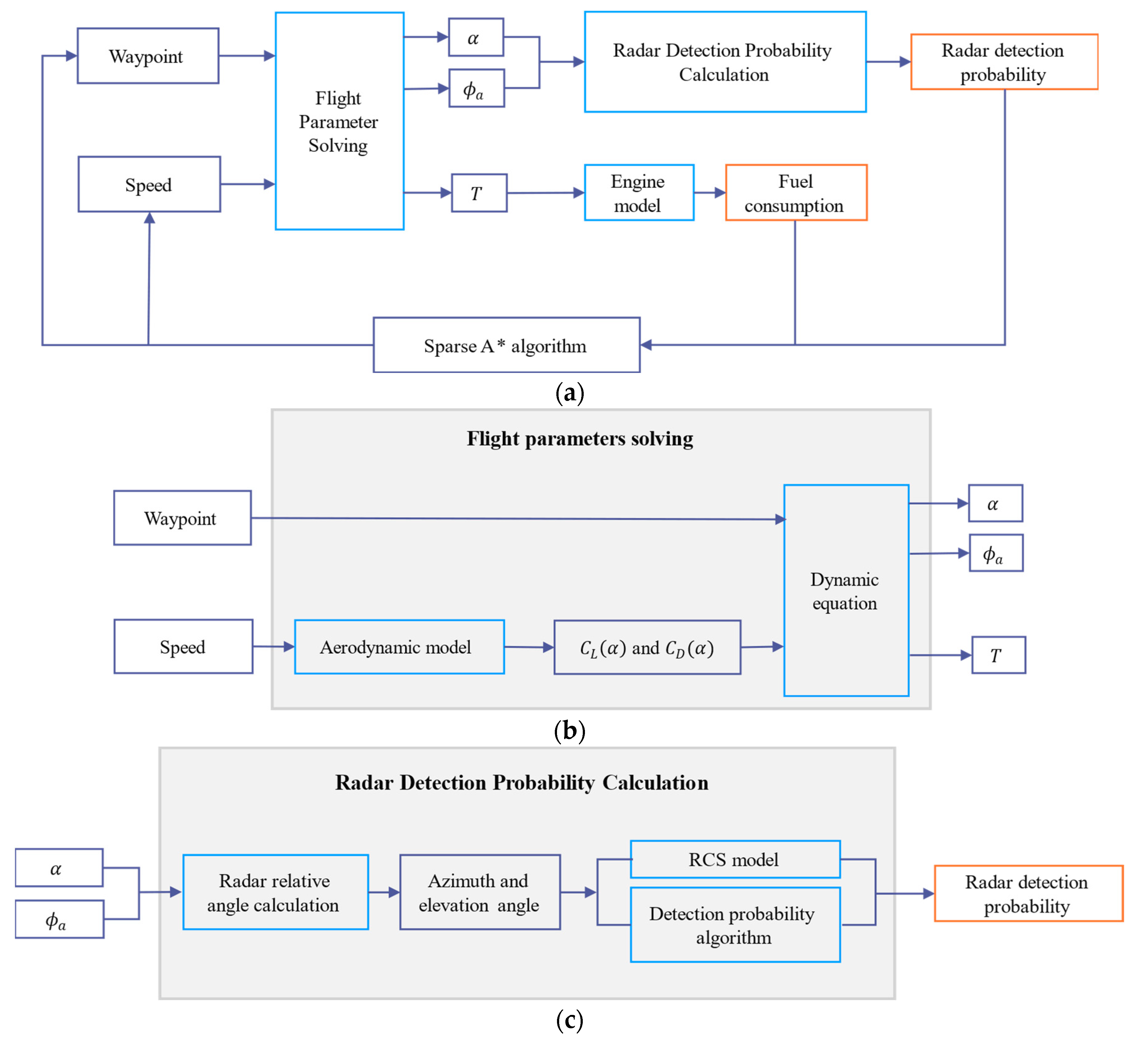
Figure 1. Flowchart of the 3D-SASLRM method: (a) overview of the 3D-SASLRM method; (b) details of the flight-parameter-solving section; (c) details of the radar probability calculation section.
Aerospace 11 00087 g001
Figure 2. The 3D RCS of a typical stealth aircraft.
Aerospace 11 00087 g002
Figure 3. Part of RCS data for a typical stealth aircraft: (a) RCS data at a −10° elevation angle. (b) RCS data at a −5° elevation angle. (c) RCS data at a 0° elevation angle. (d) RCS data at a 5° elevation angle. (e) RCS data at a 10° elevation angle.
Aerospace 11 00087 g003
Figure 4. Fitting results of the log standard and log mean for part of the RCS data: (a,b) fitting results at a −10° elevation angle; (c,d) fitting results at a −5° elevation angle; (e,f) fitting results at a 0° elevation angle; (g,h) fitting results at a 5° elevation angle; (i,j) fitting results at a 10° elevation angle.
Aerospace 11 00087 g004aAerospace 11 00087 g004b
Figure 5. Grid generation in 3 × 3.
Aerospace 11 00087 g005
Figure 6. Threat scenario for single radar.
Aerospace 11 00087 g006
Figure 7. RCS along the trajectory before planning.
Aerospace 11 00087 g007
Figure 8. Azimuth and elevation angles of the trajectory before planning: (a) azimuth angle; (b) elevation angle.
Aerospace 11 00087 g008
Figure 9. Detection probabilities of trajectory before planning in scenarios with low-power, medium-power and high-power radars: (a) low power; (b) medium power; (c) high power.
Aerospace 11 00087 g009
Figure 10. Results of the planned trajectory under low-power, medium-power and high-power radars: (a) planned trajectory under low-power radar and partially magnified at positions A and B; (b) planned trajectory under medium-power radar; (c) planned trajectory under high-power radar.
Aerospace 11 00087 g010
Figure 11. Results of the planned height under low-power, medium-power and high-power radars: (a) low-power; (b) medium-power; (c) high-power.
Aerospace 11 00087 g011
Figure 12. Azimuth angles of the planned trajectory under low-power, medium-power and high-power radars: (a) low-power; (b) medium-power; (c) high-power.
Aerospace 11 00087 g012
Figure 13. Elevation angles of the planned trajectory under low-power, medium-power and high-power radars: (a) low-power; (b) medium-power; (c) high-power.
Aerospace 11 00087 g013
Figure 14. Detection probabilities of the planned trajectory under low-power, medium-power and high-power radars: (a) low-power; (b) medium-power; (c) high-power.
Aerospace 11 00087 g014
Figure 15. Threat scenario for three-radar environment.
Aerospace 11 00087 g015
Figure 16. RCS along the trajectory before planning.
Aerospace 11 00087 g016
Figure 17. Azimuth and elevation angles of the trajectory before planning: (a) azimuth angle; (b) elevation angle.
Aerospace 11 00087 g017
Figure 18. Detection probability of the trajectory before planning under low-power, medium-power and high-power radars: (a) low power; (b) medium power; (c) high power.
Aerospace 11 00087 g018
Figure 19. Results of planned trajectory under low-power, medium-power and high-power radars: (a) planned trajectory under low-power radar and partially magnified at position A and B; (b) planned trajectory under medium-power radar; (c) planned trajectory under high-power radar.
Aerospace 11 00087 g019
Figure 20. Results of planned height under low-power, medium-power and high-power radars: (a) low power; (b) medium power; (c) high power.
Aerospace 11 00087 g020
Figure 21. Azimuth angles of the planned trajectory under low-power, medium-power and high-power radars: (a) low power; (b) medium power; (c) high power.
Aerospace 11 00087 g021
Figure 22. Elevation angles of the planned trajectory under low-power, medium-power and high-power radars: (a) low power; (b) medium power; (c) high power.
Aerospace 11 00087 g022
Figure 23. Detection probabilities of the planned trajectory under low-power, medium-power and high-power radars: (a) low-power; (b) medium-power; (c) high-power.
Aerospace 11 00087 g023
Figure 24. Danger zone determined by high-power radar valley radius.
Aerospace 11 00087 g024
Figure 25. Threat scenario for ten-radar environment.
Aerospace 11 00087 g025
Figure 26. RCS along the trajectory before planning.
Aerospace 11 00087 g026
Figure 27. Azimuth and elevation angles of the trajectory before planning: (a) azimuth angle; (b) elevation angle.
Aerospace 11 00087 g027
Figure 28. Detection probabilities of the trajectory before planning under low-power, medium-power and high-power radars: (a) low-power; (b) medium-power; (c) high-power.
Aerospace 11 00087 g028
Figure 29. Results of the planned trajectory under low-power and medium-power radars: (a) planned trajectory under low-power radars and partially magnified at position A and B; (b) planned trajectory under medium-power radars.
Aerospace 11 00087 g029
Figure 30. Results of the planned height under low-power and medium-power radars: (a) low power; (b) medium power.
Aerospace 11 00087 g030
Figure 31. Azimuth angles of the planned trajectory under low-power and medium-power radars: (a) low power; (b) medium power.
Aerospace 11 00087 g031
Figure 32. Elevation angles of the planned trajectory under low-power and medium-power radars: (a) low power; (b) medium power.
Aerospace 11 00087 g032
Figure 33. Detection probabilities of the planned trajectory under low-power and medium-power radars: (a) low power; (b) medium power.
Aerospace 11 00087 g033
Figure 34. Danger zone determined by high-power radar valley radius.
Aerospace 11 00087 g034
Figure 35. An attempt to circumvent high-power radars: (a) penetration scene and planned trajectory; (b) partial magnification of trajectory.
Aerospace 11 00087 g035
Figure 36. Detection probability of trajectory.
Aerospace 11 00087 g036
Table 1. Parameters of low-power, medium-power and high-power radars.
Radar TypePower FactorSingle Valley Radius (km)
Low power 5 × 10 5 16
Medium power 1 × 10 4 20
High power 3.9063 × 10 3 50
Table 2. Radar parameters for single-radar threat environment.
IndexLocation T s c a n (s) P F A N ρ V H R H
1(0, 50, 0)4 1 × 10 6 20.500
Table 3. Parameters for sparse A* algorithm.
Radar TypeStep Size (km)Lateral Angle (°)Upward/Downward Angle (°)Number of Expanded Nodes Weights   ( k 1 , k 2 , k 3 , k 4 , k 5 )
Low power380.59( 0 , 1 × 10 4 , 8 × 10 1 , 0 , 0 )
Medium power380.59( 1 × 10 6 , 1 × 10 4 , 8 , 0 , 1 × 10 2 )
High power380.59( 1 × 10 9 , 1 × 10 4 , 8 × 10 , 0 , 9.5 × 10 )
Table 4. Detection probabilities before and after planning under different radar powers.
Radar TypeDetection Probability
before Planning
Detection Probability
after Planning
Percentage Point Reduction in Detection Probability
Low power43.2%0.90%97.9%
Medium power88.2%0.17%99.8%
High power100.0%0.28%99.7%
Table 5. Radar parameters for three-radar threat environment.
IndexLocation T s c a n (s) P F A N ρ V H R H
1(−60, −60, 0)4 1 × 10 6 20.500
2(−10, 50, 0)4 1 × 10 6 20.500
3(60, −65, 0)4 1 × 10 6 20.500
Table 6. Parameters for sparse A* algorithm.
Radar TypeStep Size (km)Lateral Angle (°)Upward/Downward Angle (°)Number of Expanded Nodes Weights   ( k 1 , k 2 , k 3 , k 4 , k 5 )
Low power380.59( 0 , 1 × 10 4 , 8 , 1 , 1 × 10 2 )
Medium power380.59( 1 × 10 4 , 5 × 10 4 , 8 × 10 1 , 1 , 2 × 10 )
High power380.59( 1 × 10 8 , 1 × 10 3 , 8 , 1 , 1.3 × 10 2 )
Table 7. Detection probabilities before and after planning for different radar powers.
Radar TypeDetection Probability
before Planning
Detection Probability
after Planning
Percentage Point Reduction in Detection Probability
Low power42.0%0.57%98.6%
Medium power91.7%7.82%91.5%
High power100.0%4.20%95.8%
Table 8. Radar parameters for ten-radar threat environment.
IndexLocation T s c a n (s) P F A N ρ V H R H
1(−80, 120, 0)4 1 × 10 6 20.500
2(−80, 80, 0)4 1 × 10 6 20.500
3(−80, 50, 0)4 1 × 10 6 20.500
4(−80, −80, 0)4 1 × 10 6 20.500
5(100, 100, 0)4 1 × 10 6 20.500
6(100, 50, 0)4 1 × 10 6 20.500
7(100, −60, 0)4 1 × 10 6 20.500
8(−180, 150, 10)4 1 × 10 6 20.520010
9(−180, 80, 10)4 1 × 10 6 20.520010
10(−180, −120, 10)4 1 × 10 6 20.520010
Table 9. Parameters for sparse A* algorithm.
Radar TypeStep
Size (km)
Lateral Angle (°)Upward/Downward Angle (°)Number of Expanded Nodes Weights   ( k 1 , k 2 , k 3 , k 4 , k 5 )
Low power380.59( 0 , 1 × 10 4 , 10 , 1 , 0 )
Medium power380.59( 1 × 10 6 , 1 × 10 3 , 2 × 10 , 1 , 1 × 10 )
High power380.59No solution
Table 10. Detection probabilities before and after planning for different radar powers.
Radar TypeDetection Probability
before Planning
Detection Probability
after Planning
Percentage Point Reduction in Detection Probability
Low power56.0%0.98%98.3%
Medium power99.8%3.00%97.0%
High power100.0%No solutionNo solution
Table 11. Summary of the simulation results.
ScenarioRadar TypeDetection Probability
before Planning
Detection Probability
after Planning
Percentage Point Reduction in Detection Probability
1Low power43.2%0.90%97.9%
Medium power88.2%0.17%99.8%
High power100.0%0.28%99.7%
2Low power42.0%0.57%98.6%
Medium power91.7%7.82%91.5%
High power100.0%4.20%95.8%
3Low power56.0%0.98%98.3%
Medium power99.8%3.00%97.0%
High power100.0%No solutionNo solution
Disclaimer/Publisher’s Note: The statements, opinions and data contained in all publications are solely those of the individual author(s) and contributor(s) and not of MDPI and/or the editor(s). MDPI and/or the editor(s) disclaim responsibility for any injury to people or property resulting from any ideas, methods, instructions or products referred to in the content.