Article

An Improved Approach for Reducing the Dimensionality of Wing Aerodynamic Optimization Considering Longitudinal Stability

1
School of Aeronautic Science and Engineering, Beihang University, Beijing 100191, China
2
Macao Institute of System Engineering, Macau University of Science and Technology, Macau SAR, China
*
Author to whom correspondence should be addressed.
Aerospace 2024, 11(1), 80; https://doi.org/10.3390/aerospace11010080
Submission received: 1 December 2023 / Revised: 8 January 2024 / Accepted: 10 January 2024 / Published: 16 January 2024
(This article belongs to the Section Aeronautics)

Abstract

:
The wing aerodynamic shape optimization is a typical high-dimensional problem with numerous independent design variables. Researching methods to reduce the dimensionality of optimization from the perspective of aerodynamic characteristics is necessary. One traditional aerodynamic-based approach decouples the wing’s camber and thickness according to the thin airfoil theory, but it has limitations due to unclear application scope and effectiveness. This paper proposes an improved approach that determines the values of certain thickness variables based on a data-driven aerodynamic characteristics model before optimization, which considers longitudinal stability. By reducing the number of design variables, the dimensionality of optimization is decreased effectively. The derivation of the improved approach is accomplished through the design of experiments, parametric modeling, computational fluid dynamics, and sensitivity analysis. The effectiveness of the improved approach is validated by applying it to the aerodynamic optimization of an ONERA-M6 wing in subsonic flow based on the surrogate-based optimization algorithm. The results demonstrate that the improved approach significantly accelerates the optimization process while maintaining global effectiveness.

1. Introduction

Aerodynamic analysis and optimal design methodologies based on high-fidelity computational fluid dynamics have become widespread in modern aircraft design with the development of high-performance computing [1,2,3]. Currently popular optimization algorithms for aerodynamics:
  • Gradient-based algorithm
    (e.g., Sequential quadratic programming algorithm (SQP), BFGS quasi-Newton algorithm, conjugate gradient algorithm, etc.)
    This type of optimization algorithm has a fast solution speed. Combining with the adjoint method [4,5,6] can effectively solve the wing aerodynamic optimization problem at high subsonic and transonic cruise conditions [7,8,9]. However, for addressing multi-extremum problems, it is possible to fall into a local optimum due to the algorithm’s inherent limitations.
  • Gradient-free algorithm
    (e.g., Genetic algorithm (GA), simulated annealing method (SA), particle swarm optimization algorithm (PSO), etc.)
    Some of these optimization algorithms have proved their good global search capabilities in practice. Nonetheless, these algorithms require a great deal of aerodynamic evaluation during optimization, which will significantly increase the time and resource cost [10].
The surrogate-based optimization method (SBO) [11,12,13,14] arose for the purpose of enhancing optimization effectiveness and global search capability. Initially, this method builds a surrogate model based on limited discrete samples to obtain continuous samples and then searches for the optimum through traditional optimization methods. With the deepening of the research, an optimization algorithm based on historical data to drive the addition of new samples [15,16] and continuously reconstruct the surrogate model to approach the local or global optimal solution has been formed [3,17,18,19,20,21]. This method can not only enhance optimization efficiency and minimize computing costs but also help eliminate numerical noise [22].
With the continuous advancement of aircraft design concepts and the continuous improvement of design criteria, the number of independent design variables describing the shape of the aircraft in aerodynamic optimization is increasing. Aerodynamic optimization has steadily evolved into a typical high-dimensional optimization problem, and the “curse of dimensionality” increases the computational cost of optimization [23,24]. There are several potential solutions:
  • Develop optimization strategies to enhance high-dimensional problem adaptability
    Introducing low-fidelity sample data [25,26,27,28,29] or gradient information [30,31,32,33] into the surrogate-based optimization algorithm to establish the surrogate model has been proven effective. Combining parallel computing technology to develop a parallel infilling strategy [34,35,36] to maximize the usage of high-performance computers’ large-scale parallel computing capabilities
  • Research into methods to reduce the dimensionality of optimization problems
Methods to reduce the dimensionality of aerodynamic optimization problems can be classified into two categories in principle:
  • Methods based on the analysis of data
    Variable screening can minimize the number of design variables by finding the most pertinent variables to the design problem and eliminating those that are less pertinent [37,38]. However, this method reduces the design space, and correlations of omitted variables may surface later in the optimization.
    Dimensionality reduction [39] can capture potential patterns in variables in a reduced space without deleting any variables, therefore enabling optimization to be performed in a reduced space [40,41,42,43]. Some nonlinear dimensionality reduction methods [44,45] are also progressively applied to aerodynamic optimization
  • Methods based on aerodynamic characteristics
    One is the camber-thickness decoupling based on the thin-wing theory [46]. The effects of camber and thickness are considered separately in the optimization [47,48]. However, this method has shortcomings in the clarity of the application scope and the efficacy of efficiency enhancement.
The longitudinal stability of an aircraft is crucial for safety, control performance, and flight efficiency. In aerodynamic optimization, longitudinal moment constraints should be met to satisfy trim requirements. The position of the center of gravity (CG) is one of the dominant factors determining the magnitude of the longitudinal moment. For aerodynamic optimization of a fixed layout, a fixed CG position is commonly employed. However, in cases where there are local shock waves on the upper/lower surfaces of the wing, or the layout is not fixed, using a fixed CG position can lead to performance loss and deviation from expected longitudinal stability. In such scenarios, it is advisable to adopt a fixed static margin approach or consider the CG position as one of the design variables [7]. This allows for dynamic adjustment of the CG position to meet static margin requirements during the optimization process.
The main contribution of the current paper is to develop an effective method from the perspective of aerodynamic characteristics for reducing the dimensionality of wing aerodynamic optimization problems at cruise conditions.
This paper is organized as follows. In Section 2, the traditional method based on camber-thickness decoupling and the proposed improved approach are described. The methodologies employed in the aerodynamic optimization and sensitivity analysis of variance are introduced and discussed. In Section 3, the feasibility of the traditional method is analyzed, and the influence of design variables in the objective function and the main constraint function is investigated in the preliminary. In Section 4, a data-driven aerodynamic characteristics model is established through decoupling analysis, and the derivation of the improved approach is completed. In Section 5, the proposed improved approach is demonstrated by the surrogate-based aerodynamic optimization of an ONERA-M6 wing in subsonic flow. Finally, the conclusion is presented in Section 6.

2. Methodology

2.1. Geometric Parameterization

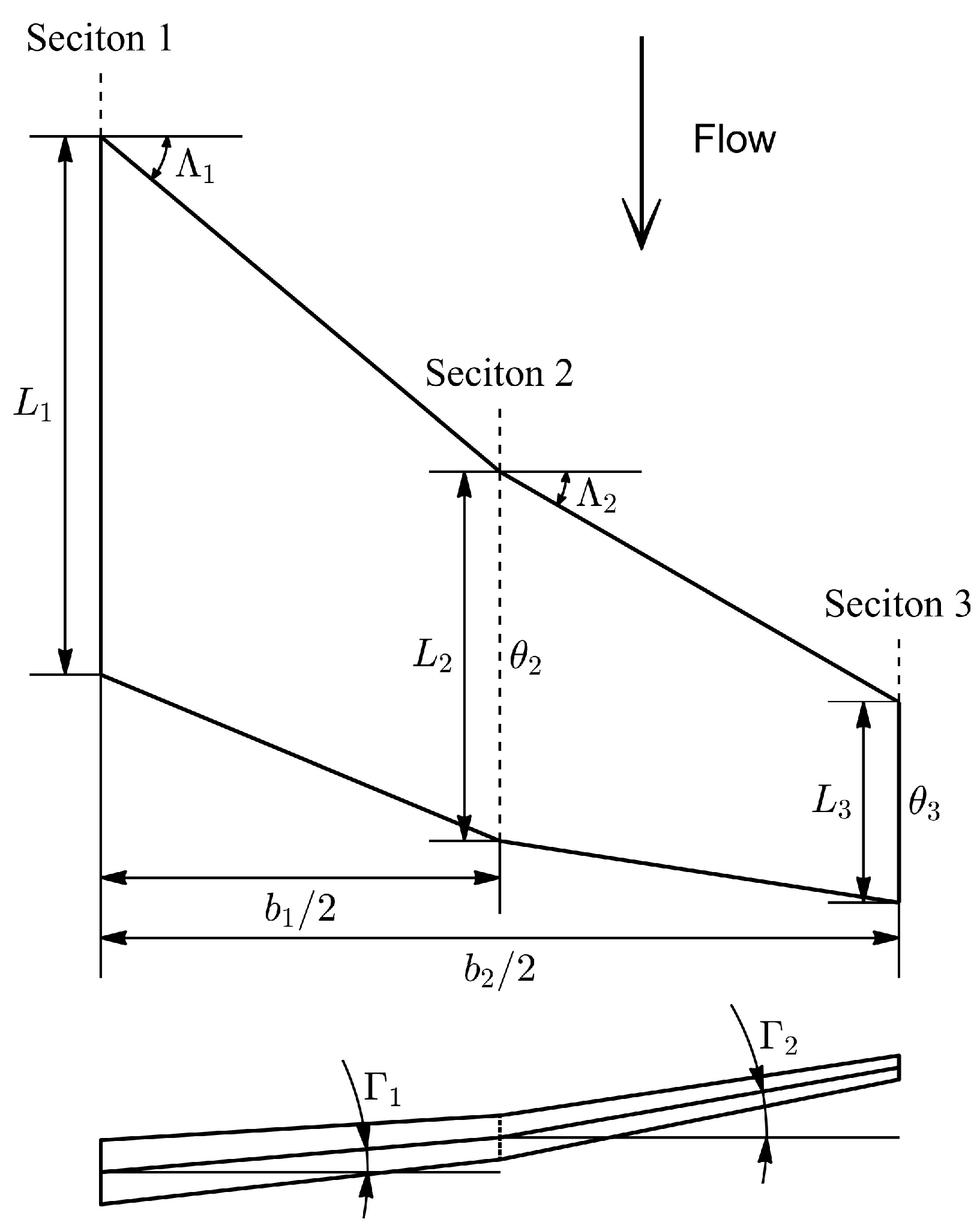
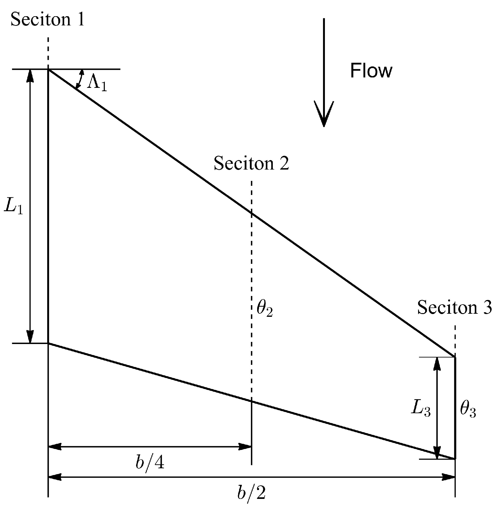
The wing planform is described by the following parameters: half-wingspan ( b / 2 ), chord length ( L ), leading-edge sweep angle ( Λ ), twist angle ( θ ), and dihedral angle ( Γ ). Figure 1 depicts the parametric modeling of a common wing planform, and the number of wing sections varies on demand.
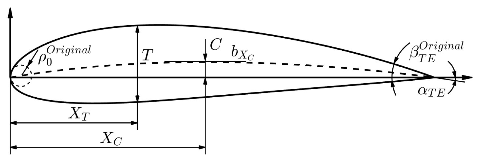
The shape of the wing section is described by the improved geometric parameter (IGP) airfoil parameterization method [49], which realized camber-thickness decoupling so that camber and thickness could be constructed separately with the following 8 geometric parameters. These parameters are illustrated in Figure 2.
Camber parameters:
  • Chordwise location of the maximum camber ( X C )
  • Maximum camber ( C )
  • Camber line curvature on the location of maximum camber ( b X C )
  • The angle between the camber line and the chord line on the trailing edge ( α T E )
Thickness parameters:
  • Chordwise location of the maximum thickness ( X T )
  • Maximum thickness ( T )
  • Dimensionless quantity of the leading-edge radius ( ρ 0 = ρ 0 O r i g i n a l / ( T / X T ) 2 )
  • Dimensionless quantity of the trailing edge boat-tail angle ( β T E = β T E O r i g i n a l / arctan ( T / ( 1 X T ) ) )
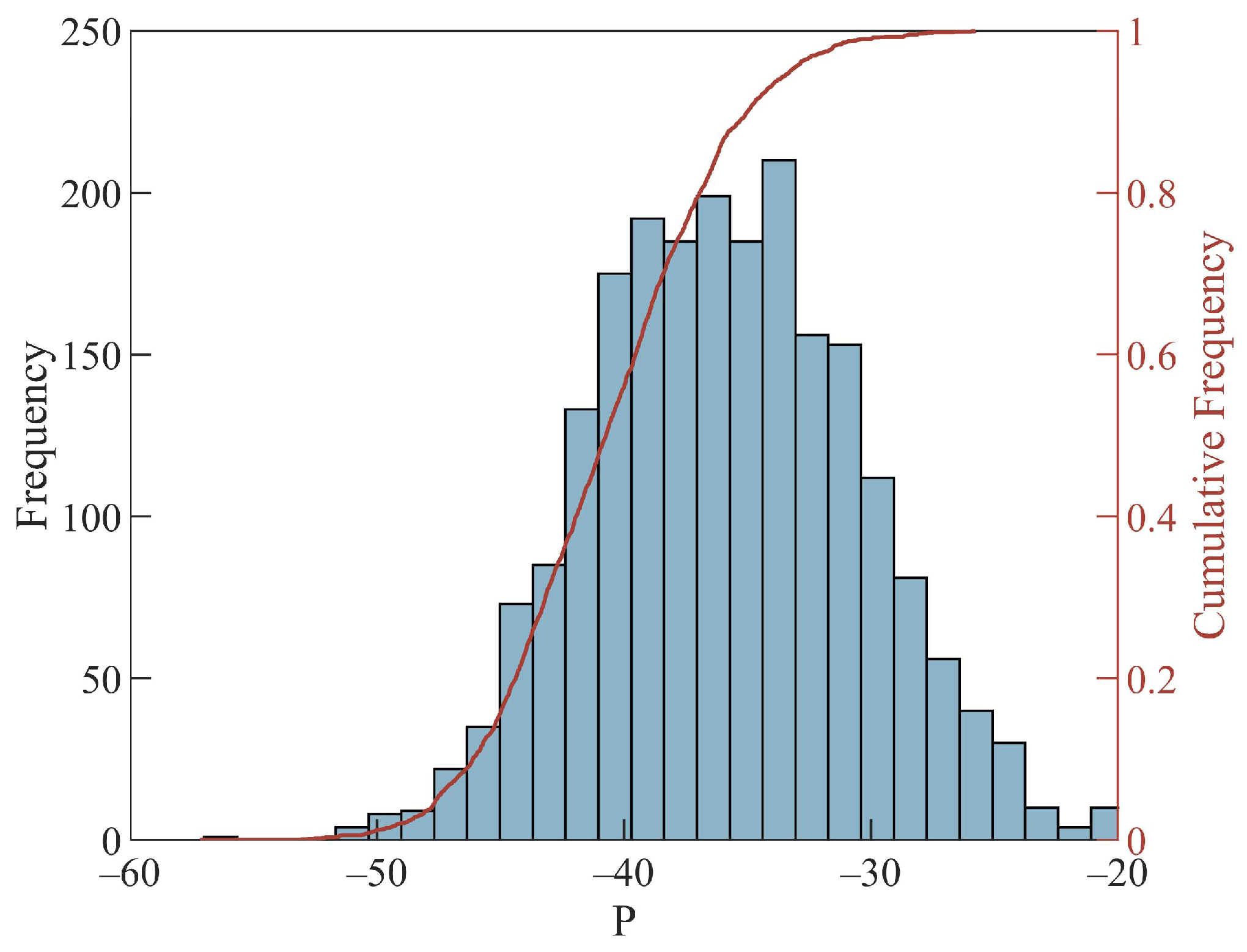
In practical application, the camber parameters evolve into 4 parameters of the curve that control the camber line. To verify the effectiveness of the IGP method, this method is applied to fit 2174 airfoils in the Profili airfoil library (which contains most of the airfoils in the UIUC airfoil database). Figure 3 shows the fitted result. The abscissa represents the value of P . The left ordinate and histogram represent the frequency of P . The right ordinate and curve represent the cumulative relative frequency of P . P is defined as:
P = 10 l o g 10 ( 1 R 2 )
where R = c o v ( y o r i   , y f i t ) / ( σ y o r i σ y f i t ) . y o r i   is the ordinate of the original airfoil in the Profili airfoil library. y f i t is the ordinate of the fitted airfoil. σ is the variance. c o v is the covariance.
The IGP method offers a good match for the entire library of airfoils. All 2174 airfoils have a fitting precision R 2 of 0.99 ( P = 20 ).

2.2. Problem Definition and Methods for Reducing Dimensions

For a typical wing aerodynamic optimization problem at cruise conditions, the objective is to minimize the drag. The constraints are associated with the velocity, lift coefficient, and pitch moment.
min C D s . t .     V = V 0 ,   C L = C L , 0   C m C m , 0
With the continuous improvement of aircraft design criteria, increasing numbers of independent design variables are required to describe the wing shape in aerodynamic optimization. Consequently, wing aerodynamic optimization is a typical high-dimensional optimization problem, which results in slow optimization progress and a significant increase in high-fidelity evaluations (e.g., CFD). Researching the method for reducing dimensions from the perspective of aerodynamic characteristics is one of the most effective solutions to the aforementioned problem.

2.2.1. The Traditional Aerodynamic-Based Method Based on Camber-Thickness Decoupling

The objective function   C D and constraint function C m can be expressed as a function of design variables:
C D = f C D ( W P , C A , T H ) C m = f C m ( W P , C A , T H )
where:
  • W P = { b , L , Λ , θ , Γ } is a variable set composed of all variables that describe the wing planform.
  • C A = { X C , i , C i , b X C , i , α T E , i } is a variable set composed of all variables that describe the camber of the airfoil section, i = 1 , 2 , , n is the wing section identifier.
  • T H = { X T , i , T i , ρ 0 , i , β T E , i } is a variable set composed of all variables that describe the thickness of the airfoil section.
According to the thin airfoil theory, when the angle of attack and camber-thickness are small for an airfoil in ideal incompressible flow, the camber and thickness can be considered separately. And C L , C m is primarily determined by the angle of attack and camber.
If { W P , C A } and T H can be decoupled in the objective function C D (called “camber-thickness decoupling”) and T H hardly contributes to the constraint function C m , then the optimization can be decomposed into 2 sub-optimizations:
  • Fix T H = T H 0 and perform optimization min f C D ( W P , C A , T H 0 ) , s . t .   f C m ( W P , C A , T H 0 )
  • Under the optimal result of 1 ( W P = W P * , C A = C A * ), execute optimization min f C D ( W P * , C A * , T H )
Since C A and T H account for most design variables, a higher-dimensional optimization can be decomposed into 2 lower-dimensional optimizations through camber-thickness decoupling. However, according to our experience, this method may have the following shortcomings:
  • The application scope is uncertain because of the unclear definition of low angle of attack and small camber-thickness (Assumptions of the thin-wing theory).
  • The total time of two lower-dimensional optimizations may not be less than that of a higher-dimensional optimization.

2.2.2. The Improved Approach Based on Decoupling Analysis

Equation (3) can be expressed as:
C D = f C D ( W P , C A , T H ) = f C D ( W P , C A , X T , i , T i , ρ 0 , i , β T E , i ) C m = f C m ( W P , C A , T H )
where i = 1 , 2 , , n is the wing section identifier.
If for any values of { W P , C A } , the following properties are satisfied (the properties are derived from our experience and will be demonstrated in Section 4):
  • { X T , i } , { T i } , { ρ 0 , i } , { β T E , i } can be decoupled from each other in the objective function C D .
  • T H hardly contributes to the constraint function C m .
  • For any values of { X T , i , ρ 0 , i , β T E , i } , min ( f C D ) = f C D ( W P , C A , X T , i , min ( T i ) , ρ 0 , i , β T E , i ) .
  • For any values of { X T , i , T i , β T E , i } , min ( f C D ) = f C D ( W P , C A , X T , n , T n , min ( ρ 0 , n ) , β T E , n ) .
  • For any values of { X T , i , T i , ρ 0 , i , } , min ( f C D ) = f C D ( W P , C A , X T , n , T n , ρ 0 , n , min ( β T E , n ) ) .
Then Equation (4) can be further simplified as:
C D = f C D ( W P , C A , X T , n , min ( T n ) , min ( ρ 0 , n ) , min ( β T E , n ) ) C m f C m ( W P , C A )
Since T H accounts for most design variables and values of T n , ρ 0 , n , β T E , n can be determined before optimization, a higher-dimensional optimization can be converted into a lower-dimensional optimization. The number of reduced dimensions is 3 n (where n is the number of wing sections), and the effect of dimension reduction is amplified as the number of wing sections increases.

2.3. Aerodynamic Analysis

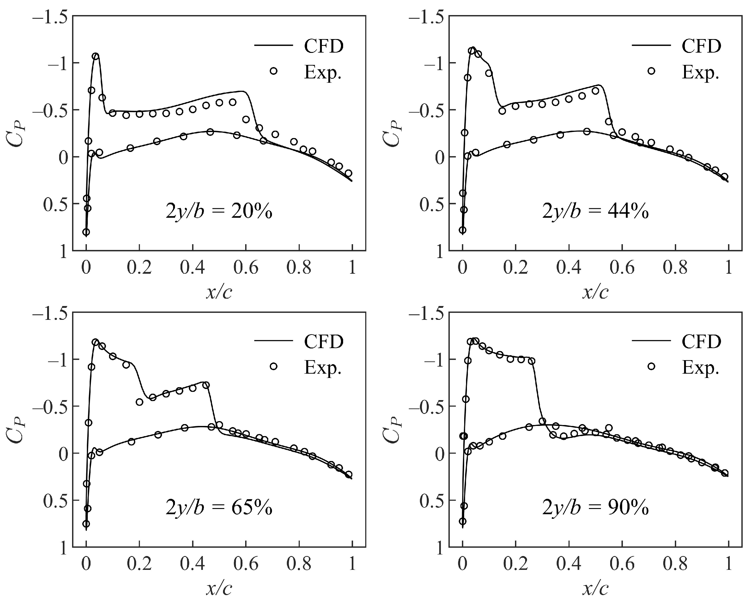
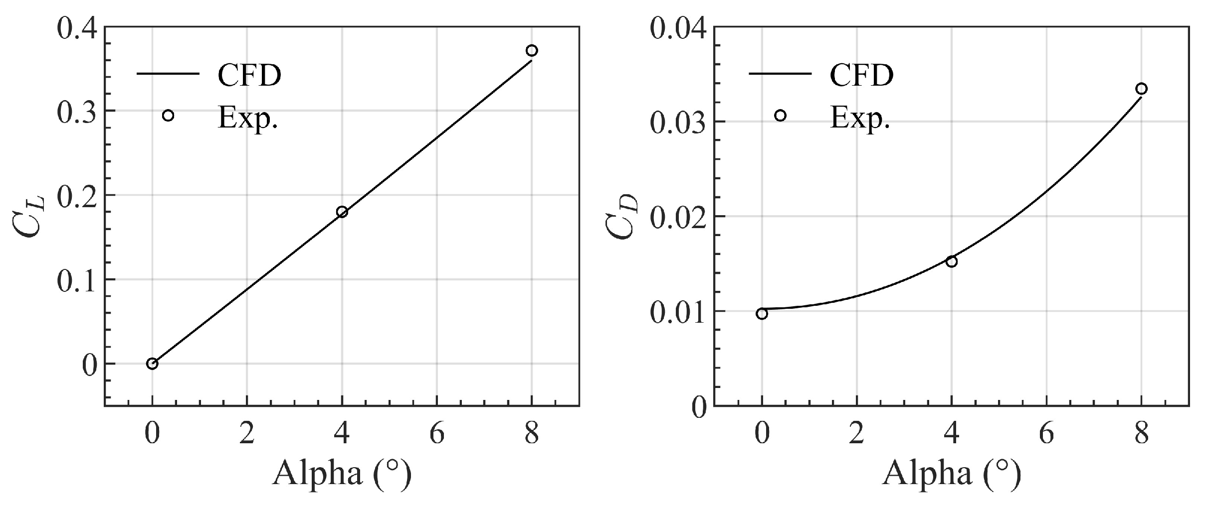
The computational fluid dynamics (CFD) method based on Reynolds-Averaged Navier–Stokes (RANS) equations with the Spalart–Allmaras turbulence model [50] is adopted for evaluating the aerodynamic characteristics. The experimental data of the ONERA-M6 wing [51] and a clean wing [52] are utilized as benchmarks to validate the accuracy of the CFD simulation. The flow condition of the ONERA-M6 wing is given by a freestream condition of M a = 0.84 , R e = 1.17 × 10 7 , α = 3.06 ° , and the flow condition of the clean wing is M a = 0.13 , R e = 1 × 10 6 . Figure 4 depicts the O-type structured mesh adopted in CFD simulation. Ensuring y + < 1 is crucial to resolve the boundary layer adequately. Figure 5 and Figure 6 demonstrate a good agreement between the CFD simulation and the experimental data.

2.4. Dynamic Adjustment of the Center of Gravity

The position of the center of gravity (CG) significantly influences the pitch moment and longitudinal stability of an aircraft. At the conceptual and preliminary design stages of an aircraft, the CG location should be optimized subject to trim and longitudinal stability constraints. The core idea of our approach is to optimize and adjust the CG position for each configuration in accordance with the specified longitudinal static stability margin ( K n ), subsequently ensuring compliance with pitch moment constraints. K n can be calculated as the ratio of the moment and lift derivatives:
K n = C m α C L a
where C m α = d C m d α , C L α = d C L d α . These can be calculated using finite differences with an angle of attack step size of 0.1 deg.
The process of dynamically adjusting the CG position can be transformed into the following sub-optimization:
min K n K n , 0 s . t . x l < x C G < x u
where K n is the static margin at any x C G , K n , 0 is the expected static margin. In all subsequent studies within this paper, this method is employed for dynamically adjusting the CG position, followed by the calculation of the pitching moment.

2.5. Surrogate-Based Optimization Algorithm

Surrogate models are mathematical models that can replace computationally complex and time-consuming numerical analysis models in analysis and optimization design. The surrogate-based aerodynamic optimization model represents a type of aerodynamic optimization method that uses surrogate modeling technologies to find the local or global best rapidly. This method cannot only significantly improve the efficiency of optimization design and reduce the complexity of engineering systems, but it can also filter out numerical noise and realize parallel optimization. With the advancement of research, a surrogate-based optimization algorithm is developed to drive the addition of new samples based on previous data and ultimately locate the local or global optimum.

2.5.1. Algorithm Framework

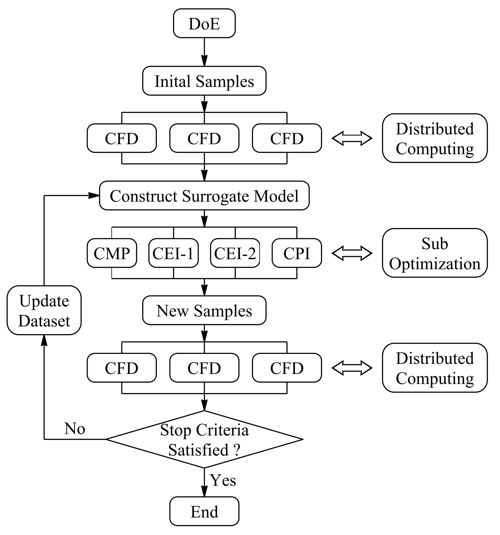
The surrogate-based optimization algorithm with a parallel infilling strategy and CFD is employed to solve the wing aerodynamic optimization problem. Figure 7 shows the flowchart.
The specific optimization process is as follows:
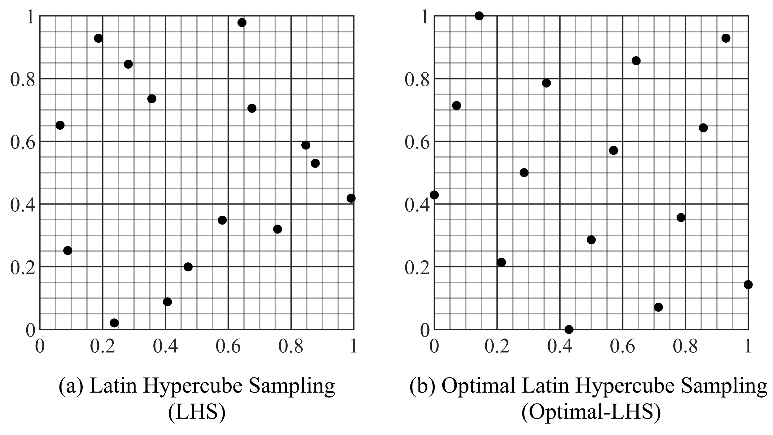
  • Generate initial samples by the design of experiments (DoE). The Optimal-LHS method derived from the LHS method ensures a high level of uniformity in design space-filling, as Figure 8 shows.
  • Evaluate samples by CFD with distributed computing, and the response values of objective and constraint functions are obtained.
  • Construct surrogate models (Kriging model).
  • According to the infill criteria [23] of CMP, CEI-1, CEI-2, and CPI (CEI-1 and CEI-2 are derived from multi-EI [34]), construct the sub-optimization problem. The traditional optimization algorithms (e.g., GA, SQP) are used to solve for new samples.
  • Evaluate new samples by CFD with distributed computing, and the response values of objective and constraint functions are obtained.
  • Return to step (3), add new samples to the dataset, and update the surrogate model. Repeat the preceding steps until the resulting sample converges to the local or global optimal solution.
We can verify the efficacy of this framework by substituting CFD optimization problems with basic functions and executing optimization.

2.5.2. Constrained Global Optimization Test Case of a G9 Function

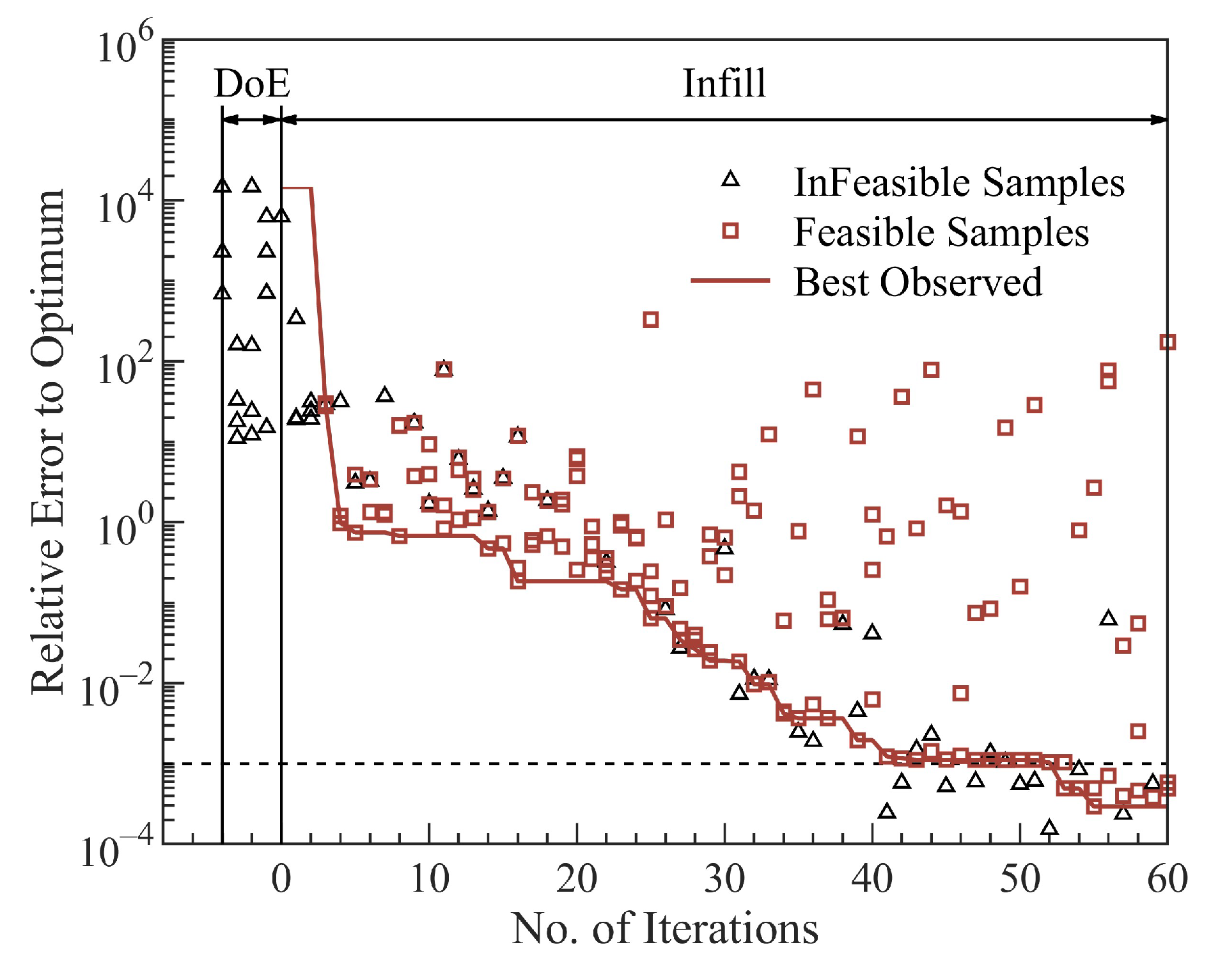
The G9 function is selected as the first test case, which is a frequently used benchmark test case to evaluate global optimization algorithms. This problem contains 7 variables and 4 constraints, and its feasible domain represents only 0.5% of the design space. The problem is described as follows:
min f ( x ) = ( x 1 10 ) 2 + 5 ( x 2 12 ) 2 + x 3 4 + 3 ( x 4 11 ) 2                                                   + 10 x 5 6 + 7 x 6 2 + x 7 4 4 x 6 x 7 10 x 6 8 x 7 w . r . t   x i = [ 10 , 10 ] ,   i = 1 , 2 , , 7 s . t .     g 1 ( x ) = 127 2 x 1 2 3 x 2 4 x 3 4 x 4 2 5 x 5 0   g 2 ( x ) = 282 7 x 1 3 x 2 10 x 3 2 x 4 + x 5 0   g 3 ( x ) = 196 23 x 1 x 2 2 6 x 6 2 + 8 x 7 0   g 4 ( x ) = 4 x 1 2 x 2 2 + 3 x 1 x 2 2 x 3 2 5 x 6 + 11 x 7 0
The known optimum of this problem:
x * = ( 2.330499 , 1.951372 , 0.4775414 , 4.365726 , 0.6244870 , 1.038161 , 1.594227 ) f ( x * ) = 680.6300573
A total of 16 initial samples are obtained by the Optimal-LHS method to begin the optimization. The convergence history of optimization is sketched in Figure 9. The results show it converges to the global minimum after 60 iterations for a total of 240 function evaluations (4 new samples generated per iteration). We consider that it can be regarded as finding the optimum when the relative error is lower than 0.1%.

2.5.3. Unconstrained Global Optimization Test Case of a Sum-Squares Function

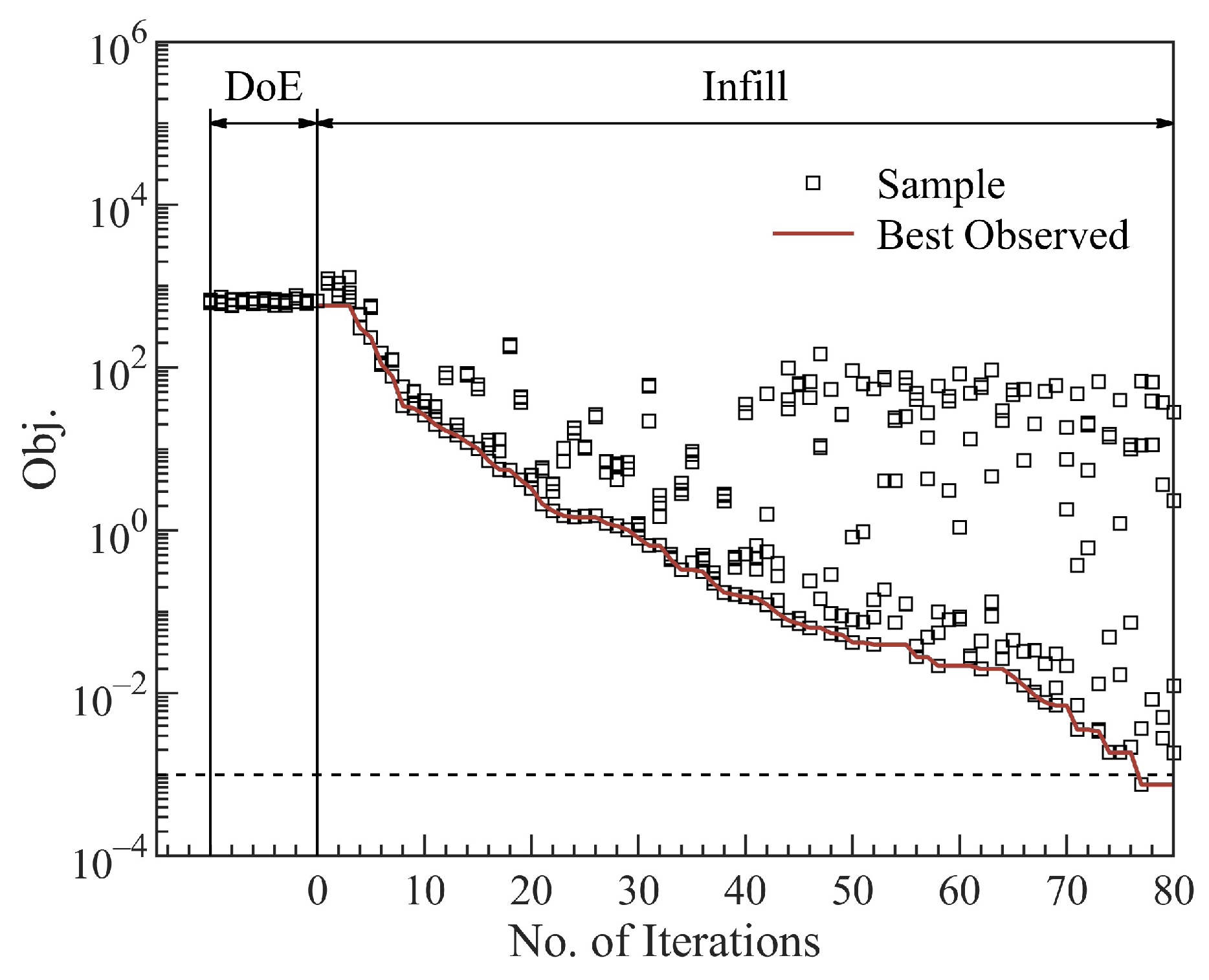
We further use the Sum-Squares function as a test case for high-dimensional optimization. This problem contains 30 variables and has no constraints, described as follows:
min   f ( x ) = i = 1 n ( i x i 2 ) w . r . t   x i = [ 2 , 2 ] ,     i = 1 , 2 , , n ,     n = 30
The true optimum of this problem: x * = [ 0 , , 0 ] ,     f ( x * ) = 0 .
A total of 40 initial samples are obtained by the Optimal-LHS method to begin the optimization. The convergence history of optimization is sketched in Figure 10. The results show it converges to the global minimum after 80 iterations for a total of 320 function evaluations (4 new samples generated per iteration). It can be regarded as finding the optimum when the objective value is lower than 0.1%.

2.6. Sensitivity Analysis of Variance

Identifying each design variable’s effect on the function is necessary before the optimization begins. Once the surrogate model ( y ^ = f ( x ) ) has been constructed, functional analysis of Variance (ANOVA) [53,54] can accomplish the aforementioned goal by decomposing the model’s total variance into that of each design variable and its interaction. This method requires the function ( y ^ = f ( x ) ) to be centralized:
0 1 f ( x t 1 , , x t k ) d t j = 0 ,   t j = 1 , , k
The total mean ( μ t o t a l ) and total variance ( σ t o t a l 2 ) of model y ^ are as follows:
μ t o t a l = f ( x 1 , , x n ) d x 1 d x n σ t o t a l 2 = f ( x 1 , , x n ) μ t o t a l 2 d x 1 d x n
The main effect of variable x i is:
S i = σ i 2 σ t o t a l 2 = μ i ( x i ) 2 d x i σ t o t a l 2
where μ i ( x i ) = f ( x 1 , , x n ) k i d x k μ t o t a l
The two-way interaction effect of variable x i , x j is:
S i , j = σ i , j 2 σ t o t a l 2 = μ i , j ( x i , j )   2 d x i d x j σ t o t a l 2
where μ i , j ( x i , j ) = f ( x 1 , , x n ) k i , j d x k μ i ( x i ) μ j ( x j ) μ t o t a l
In general, the interaction effect of variable x t 1 , , x t k is:
S t 1 t k = σ t 1 t k 2 σ t o t a l 2 = μ t 1 t k 2 d x t 1 d x t k σ t o t a l 2
The sensitivity indices ( S ) indicate the effect of design variables in the objective function. All the S t 1 t k are nonnegative, and their sum is:
k = 1 n t 1 < < t k n S t 1 t k = 1
In particular, if S 1 + + S n = 1 , that means f ( x ) is a sum of one-dimensional functions:
f ( x ) = f 0 + i = 1 n f i ( x i )
To verify the correctness of the solver, a function with separated variables is considered:
f ( x ) = i = 1 n 4 x i 2 + p i 1 + p i
where n = 8 , p 1 = p 2 = 0 , p 3 = = p 8 = 3 .
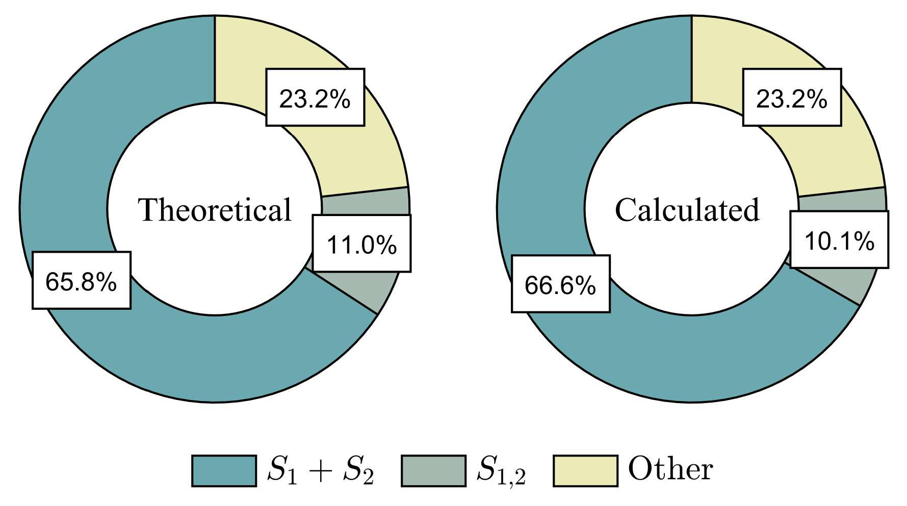
Figure 11 shows the theoretical values [54] and calculated values from our solver of the effect of design variables on function. It can be seen that the value calculated by our solver is in good agreement with the theoretical value. S 1 + S 2 means the sum of the main effect of x 1 , x 2 , S 1 , 2 means the interaction effect of x 1 , x 2 .

3. Analysis Based on the Traditional Method

The key to the traditional method is that variables describing the wing planform and sections’ camber ( { W P , C A } ) and variables describing sections’ thickness ( T H ) can be decoupled in the objective function C D , and T H hardly contributes to the constraint function C m .
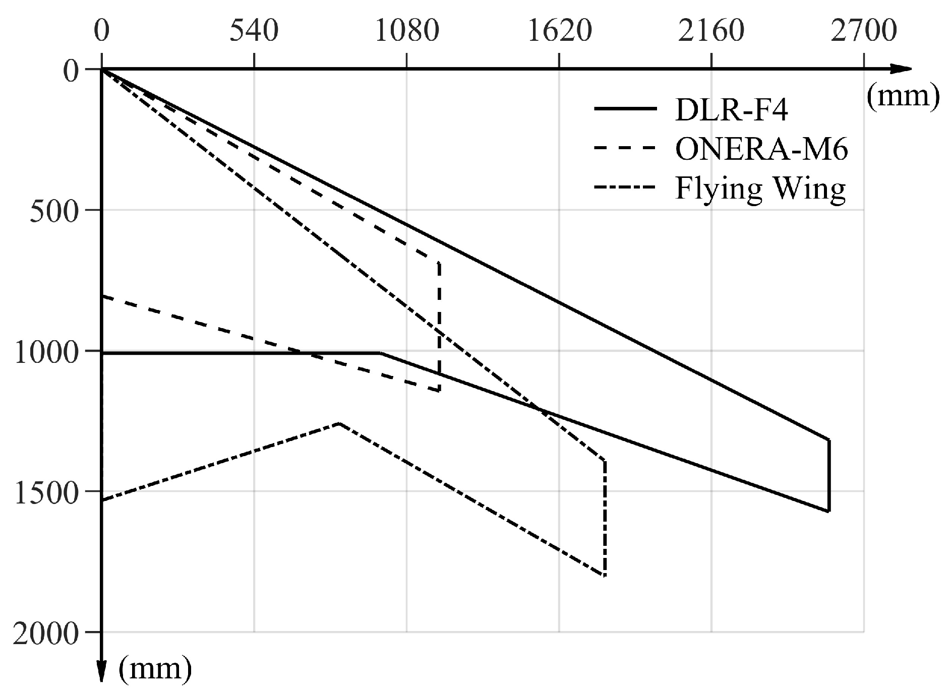
We select 3 wing planforms of DLR-F4, ONERA-M6, and a typical flying wing to investigate the coupling phenomenon of C A and T H in the objective function C D and the constraint function C m in a given V , C L , and design space. The top view of these wings is shown in Figure 12. The proportions of all wing planforms are scaled to be essentially identical, and twist and dihedral angles are eliminated.
For sections’ parametric modeling, we specify the identical airfoil for each section of each wing planform and adopt the IGP method. A wide-range and a low-range design space are used in this analysis. The wide-range design space is defined as containing about 95% airfoils in the Profili airfoil library, while the low-range design space contains about 40%. A total of 8 parameters of the IGP method are used as design variables, and the procedure of analysis is described as follows:
For each design space (wide-range and low-range):
  • Generate 300 samples by the Optimal-LHS method.
  • Evaluate each sample at 0.147 M a by CFD.
  • Define the longitudinal static stability margin K n = 3.5 % and automatically adjust the CG position. C D , C m at C L = [ 0.6 , 0.8 , 1 ] C L , L / D m a x are used as the response values to build the surrogate model:
    C D = f C D ( C A , T H ) C m = f C m ( C A , T H )
  • Based on ANOVA analysis,   S C A , S T H , S C o u p l e d in C D , C m are obtained, where:
    S C A means the sum of the main effects of C A
    S T H means the sum of the main effects of T H
    S C o u p l e d means the interaction effect between C A and T H
There are 900 samples (3 configurations × 300) per design space, and each sample needs to be evaluated for 4 angles of attack states and a specific velocity state. A total of 7200 (2 × 3 × 300 × 4) CFD evaluations are required. The CFD evaluation adopts the O-type structured mesh, with about 3 million cells in each model.
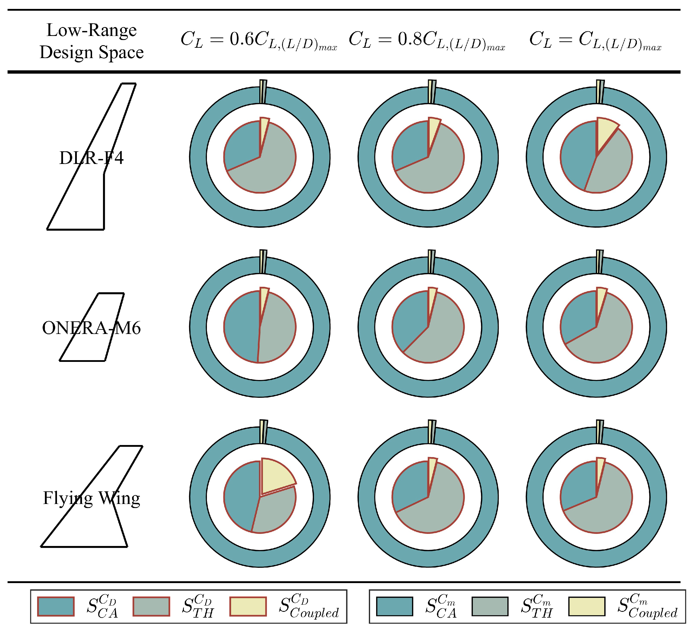
The results of wide-range and low-range design spaces are presented as pie charts in Figure 13 and Figure 14. The inner ring pie chart represents C D , and the outer pie chart represents C m . The following conclusions can be drawn:
  • In wide-range design spaces, the interaction effect between C A and T H in the objective function C D cannot be ignored.
  • In low-range design spaces, the interaction effect between C A and T H in the objective function C D appears unimportant.
  • In both wide-range and low-range design spaces, T H hardly contributes to the constraint function C m .
The shortcomings of this method are further explained as follows:
  • The applicable range is ambiguous since the definitions of low angle of attack and small camber-thickness are unclear. This section demonstrates that this method became possible due to the drastic reduction of the design space.
  • To reach the same objective, two lower-dimensional optimizations may not take less time than one higher-dimensional optimization.
  • In contrast to some rapid aerodynamic evaluation methods (e.g., vortex lattice method) that only require the data of the camber in the wing, the CFD-RANS method requires the complete data of thickness and camber. This means that before we start the first low-dimensional optimization (planform and camber optimization), we need to assign values to thickness variables for which the logic of the assignment is unclear.

4. Complete Derivation of the Improved Approach

The following steps are required to verify the preceding inference in Section 2.2.2:
  • Verify that thickness variables { X T , i } , { T i } , { ρ 0 , i } , { β T E , i } can be decoupled from each other in the objective function C D , and T H hardly contributes to the constraint function C m . Where i = 1 , 2 , , n is the wing section identifier.
  • Establishing a data-driven aerodynamic characteristics model analyzing the correlations between X T , i , T i , ρ 0 , i , β T E , i and objective function C D .
To complete the preceding steps and ensure the universality of the results, 22 configurations of wing camber surfaces without thickness (only use { W P , C A } as design variables) are generated using the geometric parameterization method and the design of experiments. The design variable and value ranges are shown in Figure 15 and Table 1.

4.1. Verification of Decoupling of Thickness Variables

A total of 12 thickness variables (3 sections, 4 thickness variables per section) are used as design variables.
For each configuration of wing camber surface (total of 22 configurations):
  • Generate 100 samples by the Optimal-LHS method.
  • Evaluate each sample at [ 0.147 , 0.3 , 0.6 ] M a by CFD.
  • C D at C L = [ 0.75 , 1 ] C L , L / D max are used as the response values to build the surrogate model:
    C D = f C D { X T , i } , { ρ 0 , i } , { ρ 0 , i } , { β T E , i }
    where i = 1 , 2 , 3 represents the wing section identifier.
  • Based on ANOVA analysis, S { X T , i } , S { T i } , S { ρ 0 , i } , S { β T E , i } in C D are obtained.
  • Define the longitudinal static stability margin K n = 3.5 % and automatically adjust the CG position. C m at C L = [ 0.75 , 1 ] C L , L / D max are used to analyze the magnitude of the influence of thickness variables on constraint function.
There are 2200 (22 configurations × 100) samples, and each sample needs to be evaluated for 4 angles of attack states and 3 velocity states. A total of 26,400 (22 × 100 × 4 × 3) CFD evaluations are required. The CFD evaluation adopts the O-type structured mesh, with about 3 million cells in each model.
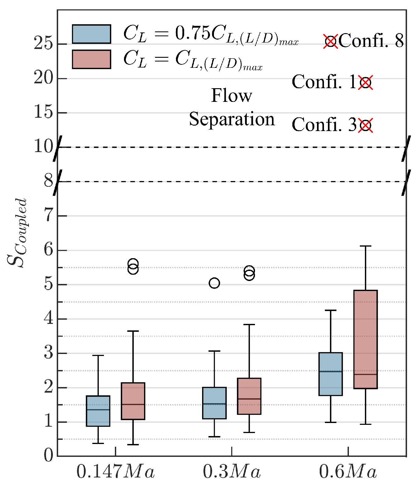
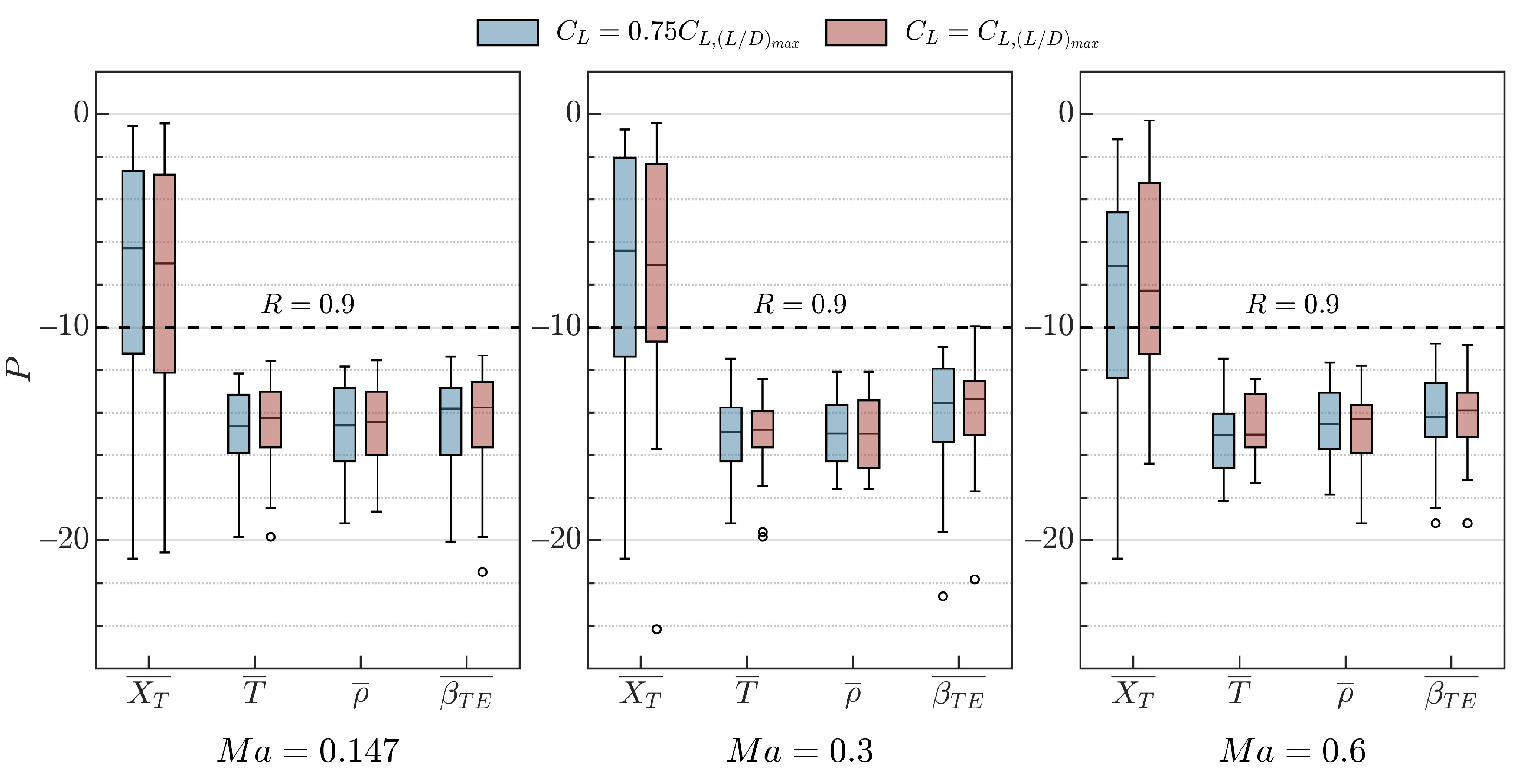
Let S C o u p l e d = 1 ( S { X T , i } + S { T i } + S { ρ 0 , i } + S { β T E , i } ) , and values of all configurations are presented in Figure 16 as a box plot. Since planform variables and camber variables of each non-thickness configuration are randomly sampled, and thickness variables overlaid on this configuration are also generated through random sampling, this can lead to the generation of unusual wing shapes. These unusual wing shapes are prone to flow separation under the given flow conditions, resulting in the occurrence of outliers that do not satisfy the decoupling conditions at 0.6 M a . Table 2 provides the flow conditions and the number of samples in which flow separation occurred during CFD aerodynamic evaluation after overlaying the thickness variable for these 22 non-thickness configurations. The criterion for evaluating the occurrence of flow separation is whether the wing surface streamlines detach from the body.
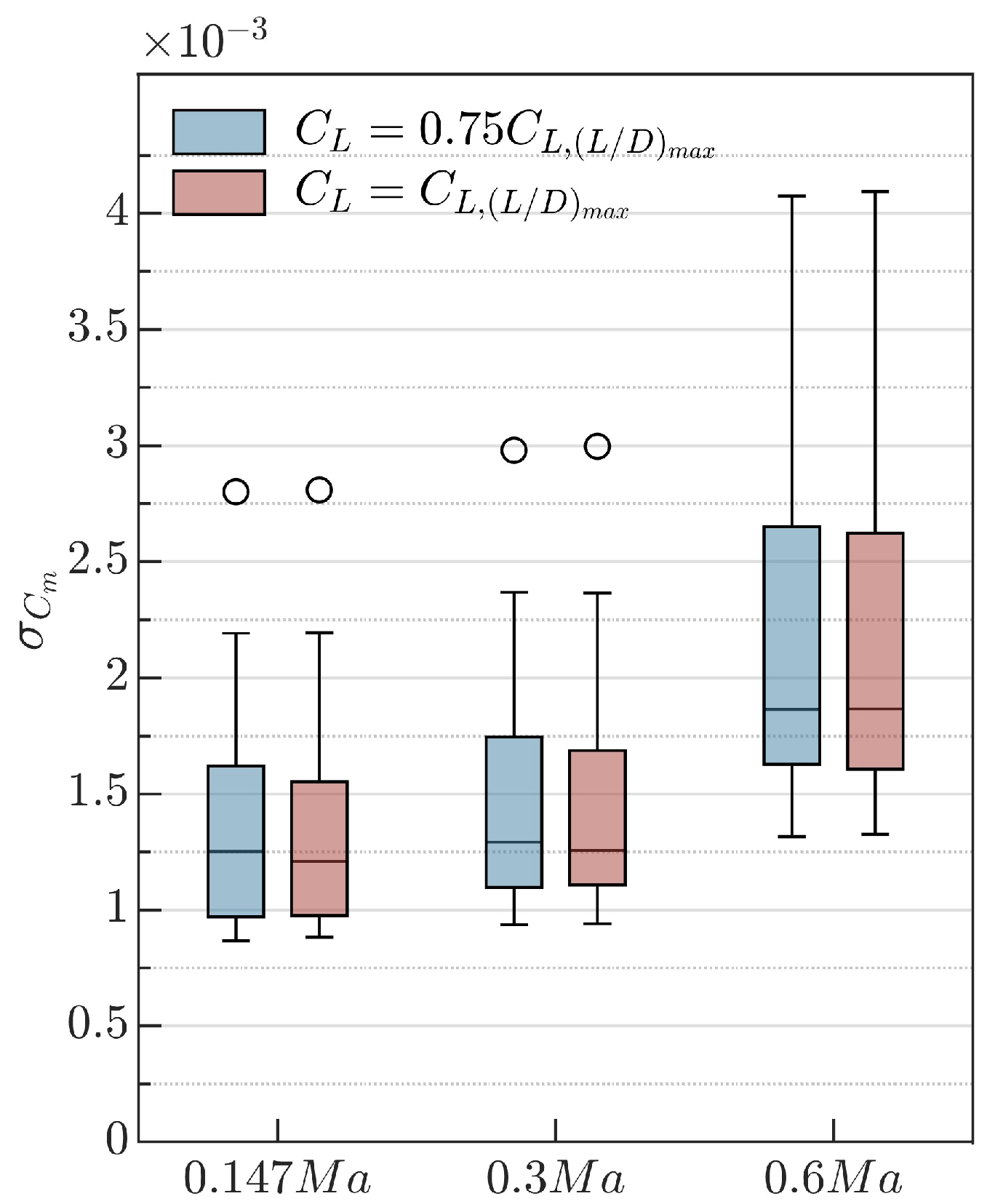
Figure 17 depicts the standard deviation of the influence of thickness variables ( T H ) on C m (Excluded configurations with airflow separation). The longitudinal static stability margin of each configuration is 3.5%, and the magnitude of the influence on C m remains at 10 3 .
From Figure 16 and Equation (16) and Figure 17, we can conclude that within the given V , C L , and design space, for any values of { W P , C A } :
  • { X T , i } , { T i } , { ρ 0 , i } , { β T E , i } can be decoupled from each other in the objective function C D . (we consider S C o u p l e d negligible below about 5%)
  • T H hardly contributes to the constraint function C m .

4.2. Establishment of the Data-Driven Aerodynamic Characteristics Model

According to the conclusions in Section 4.1, the relationship between thickness variable sets ( { X T , i } , { T i } , { ρ 0 , i } , { β T E , i } ) and objective function C D can be analyzed decoupled. We obtain the source data through the following steps to establish the data-driven aerodynamic characteristics model:
There are 4 rounds in all:
1 st round, P i = X T , i
2 nd round, P i = T i
3 rd round, P i = ρ 0 , i
4 th round, P i = β T E , i
Where i = 1 , 2 , 3 represent the wing section identifier.
In each round, for each configuration (22 configurations in total) of wing camber surface:
  • { P i } are used as design variables (3 sections, a total of 3 variables) to generate 28 samples by the Optimal-LHS method, while the remaining thickness variables are generated randomly. Combine wing camber surfaces to form wing shapes.
  • Evaluate each sample at [ 0.147 , 0.3 , 0.6 ] M a by CFD.
  • C D at C L = [ 0.75 , 1 ] C L , L / D m a x are used as the response values to build the surrogate model:
    C D = f C D ( { P i } )
  • Based on ANOVA analysis, S i in C D are obtained, where:
  • First-order fit P ¯ and C D , where:
    P ¯ = S 0 P 0 + S 1 P 1 + S 2 P 2
There are 2464 (22 configurations × 4 types of thickness variables × 28) samples, and each sample needs to be evaluated for 4 angles of attack states and 3 velocity states. A total of 29,568 (22 × 4 × 28 × 4 × 3) CFD evaluations are required. The CFD evaluation adopts the O-type structured mesh, with about 3 million cells in each model.
Figure 18 depicts the result of configuration 1 and serves as an example for later figures. The dots indicate the original data of samples, while curves show the first-order fitting result. The diagram from left to right illustrates the relationship between X T ¯ ,   T ¯ ,   ρ 0 ¯ ,   β T E ¯ and C D .
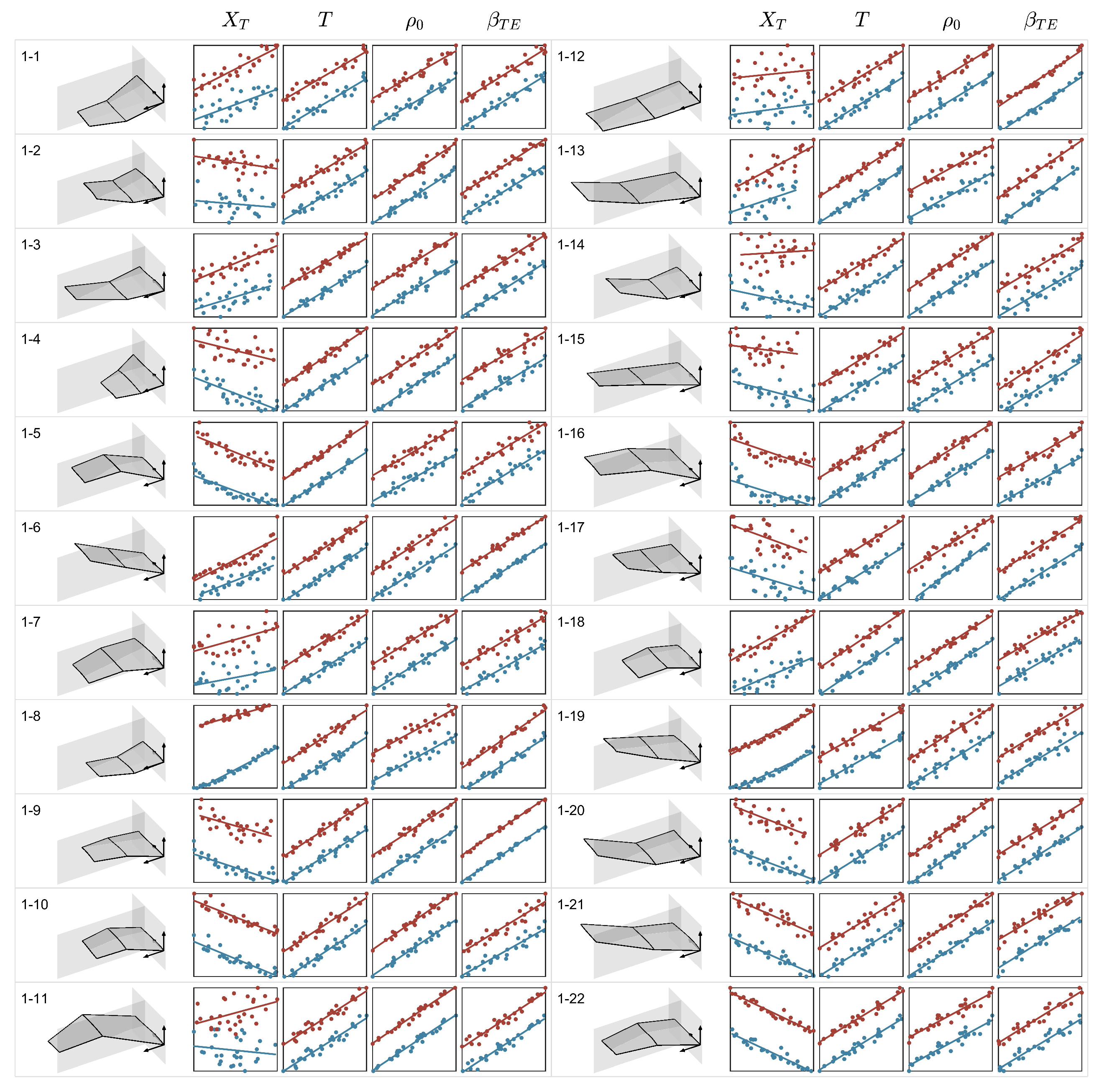
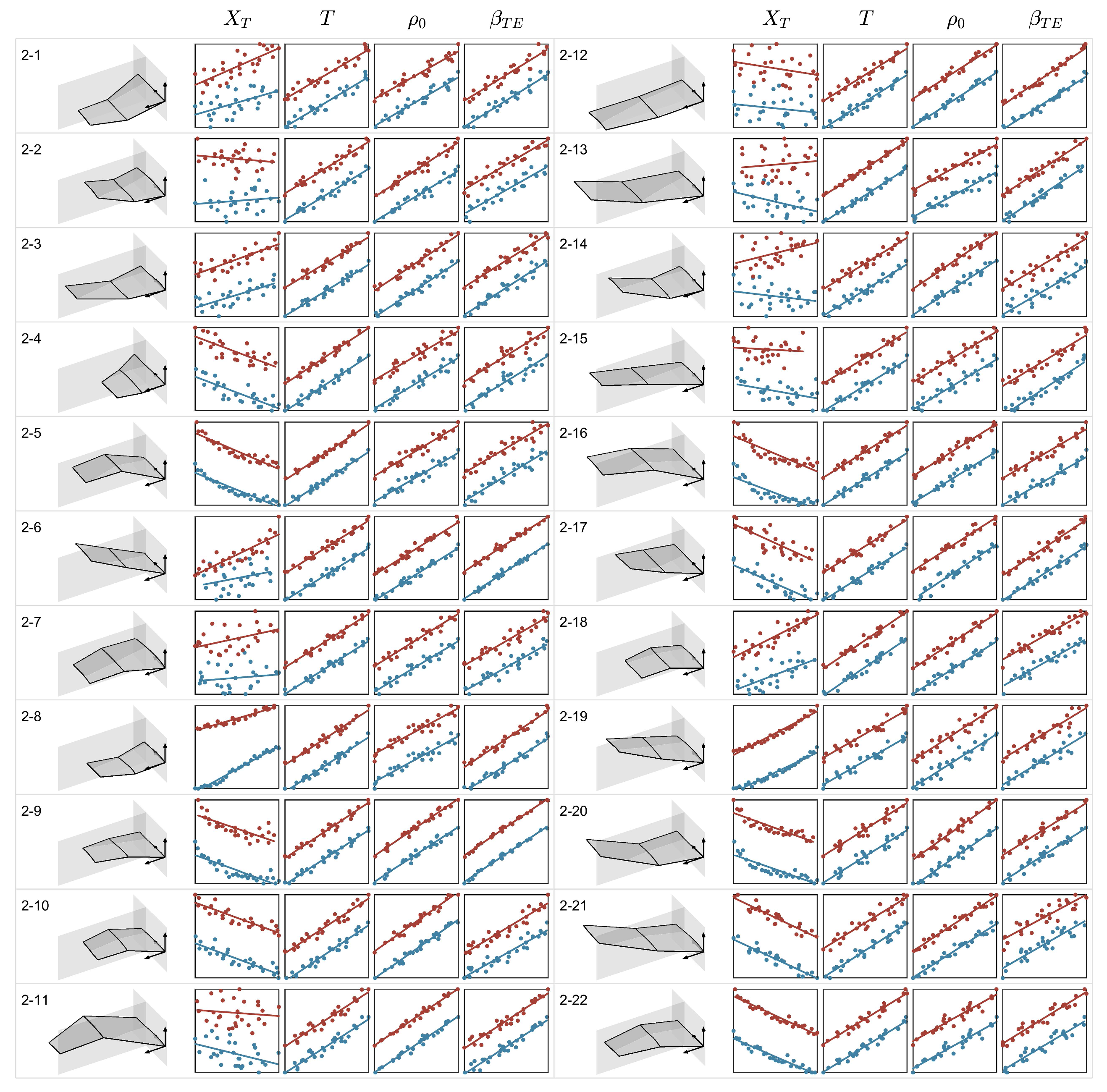
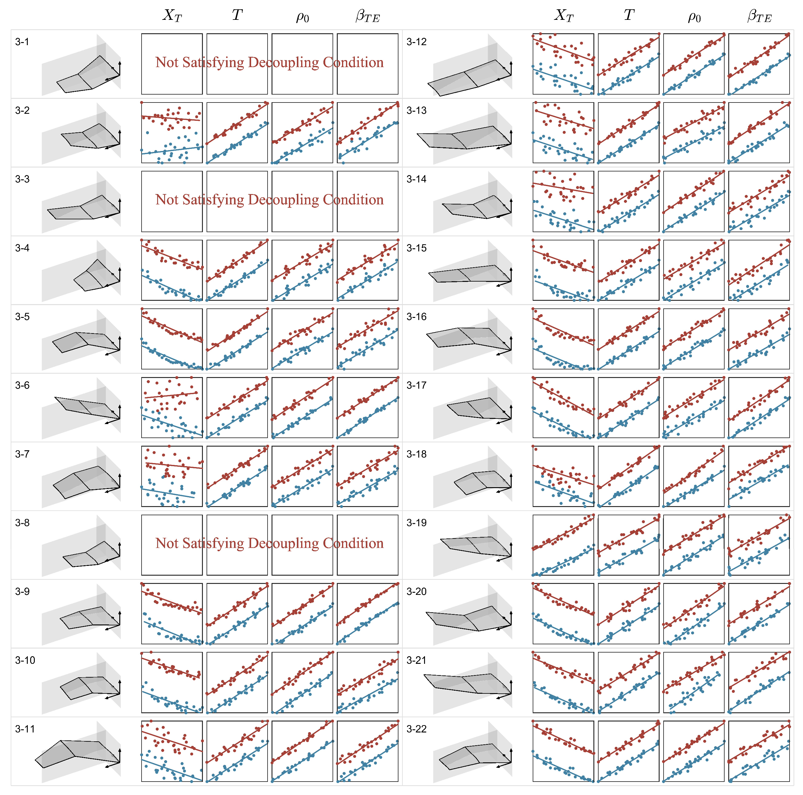
The results of all configurations at different velocities are shown in Figure 19, Figure 20 and Figure 21 (See Figure 18 for the chart format). Each figure is divided into 22 regions, each of which represents a configuration. In each region, the leftmost is the geometric shape of the configuration, while the 4 diagrams on the right illustrate the correlation between X T ¯ ,   T ¯ ,   ρ 0 ¯ ,   β T E ¯ and C D . As can be seen from the figure, the correlation between T ¯ ,   ρ 0 ¯ ,   β T E ¯ and C D of each configuration is strong and positive, while the correlation of X T ¯ is weak.
We further define the Spearman correlation coefficient ( R ) to measure the correlation. The absolute value of the correlation coefficient ( R ) is between 0 and 1. A correlation value of 1 shows a complete association, while a correlation value of 0 indicates no correlation. All results are presented in Figure 22 (where P = 10 l o g 10 ( 1 R ) ). The R of T ¯ ,   ρ 0 ¯ ,   β T E ¯ are greater than 0.9, which further illustrates the high correlation between T ¯ ,   ρ 0 ¯ ,   β T E ¯ and C D . And the R of X T ¯ range from 0 to 1, which means its correlation is weak.
From Figure 18, Figure 19, Figure 20 and Figure 21, we can conclude that within given V , C L , and design space, for any values of { W P , C A } :
  • For any values of { X T , i , ρ 0 , i , β T E , i } , min ( f C D ) = f C D ( W P , C A , X T , i , min ( T i ) , ρ 0 , i , β T E , i ) .
  • For any values of { X T , i , T i , β T E , i } , min ( f C D ) = f C D ( W P , C A , X T , n , T n , min ( ρ 0 , n ) , β T E , n ) .
  • For any values of { X T , i , T i , ρ 0 , i , } , min ( f C D ) = f C D ( W P , C A , X T , n , T n , ρ 0 , n , min ( β T E , n ) ) .
Based on the aforementioned conclusions, we can develop a data-driven aerodynamic characteristics model. In the given V , C L , and design space:
{ W P , C A } R ,   C D = f C D ( W P , C A , X T , n , min ( T n ) , min ( ρ 0 , n ) , min ( β T E , n ) ) C m f C m ( W P , C A )

4.3. Application Scope

Since it is difficult to prove the applicable boundary strictly, we provide the range based on calculation and experience. The criteria for determining the applicability of this method are as follows:
  • There is no regional flow separation on the upper and lower surfaces of the wing.
  • The coupling ( S C o u p l e d ) of { X T , i } , { T i } , { ρ 0 , i } , { β T E , i } is not greater than about 5%.
  • The correlation coefficient ( R ) between X ¯ , T ¯ , ρ 0 ¯ , β T E ¯ and objective function C D is greater than about 0.9.
The following variables have a significant impact on the applicability of this approach:
  • Mach number ( M a ) [ * , 0.147 ] [ 0.147 , 0.6 ] M a
Uncertainty of lower limit. The Reynolds number decreases as the M a decreases, which may result in more significant laminar flow effects. Higher M a may result in shock waves on the wing surface, and this airfoil parameterization method (IGP method) has poor adaptability to transonic flow due to its lack of local geometric modification capability.
  • Design lift coefficient ( C L ) [ 0.75 , 1 ] C L , L / D m a x
Lower or Higher C L results in stronger coupling between design variables in some configurations. Meanwhile, higher C L exceeds the lift coefficient at the maximum lift-drag ratio. The aircraft can easily enter the speed instability area, which is not conducive to flight control.
  • Leading-edge sweepback ( Λ ) [ 0 , 45 ] deg
Large Λ increases the equivalent angle of attack of the vertical leading edge, which more easily causes the leading-edge airflow separation.
  • The IGP method’s parameters. On the basis of design space containing 95% of the airfoils in the Profili airfoil library:
X C [ 9.6 , 87.5 ] % ,   C [ 2.7 , 6.4 ] % ,   X T [ 20 , 45 ] % ,   T [ 8 , 18 ] %
A larger camber with a smaller thickness makes it easier to cause airflow separation on the wing surface.
Please note that this method is still partially available beyond this range but may incur some performance loss that is difficult to quantify.

5. Validation by Surrogate-Based Aerodynamic Optimization

In contrast to transonic aerodynamic optimization, low subsonic aerodynamic optimization is less sensitive to the geometric shape, as demonstrated by the fact that two geometrically distinct designs can achieve almost identical aerodynamic performance under given conditions. Therefore, low subsonic optimization is a typical multi-extreme problem, necessitating an optimization method with a high global search capability. Low global search capability can easily lead to optimization results with unusable geometry. As a verification case, we select a surrogate-based low subsonic aerodynamic optimization based on the aforementioned concerns.

5.1. Determination of Full-Dimensional and Reduced-Dimensional Optimization

According to whether the improved approach is adopted, aerodynamic optimization is classified into 2 types: full-dimensional optimization and reduced-dimensional optimization. In reduced-dimensional optimization, certain thickness variables ( T ,   ρ 0 ,   β T E ) can be determined before optimization by the proposed improved approach. By comparing the full-dimensional and reduced-dimensional optimization of an ONERA-M6 wing in subsonic flow, the effectiveness of the improved approach can be verified.
The optimization problem is stated below as Equation (23). The objective is to minimize the drag. The constraints are associated with the velocity, lift coefficient, pitch moment (longitudinal static stability margin is set to 3.5%), area of the wing, maximum thickness, and dimensionless quantity of the trailing edge boat-tail angle of all wing sections. The design variables and their value ranges are depicted in Figure 23 and Table 3.
min C D s . t .     V = 0.147 M a ,   C L = 0.3   C m 0.03   S w S w , 0 / S w , 0 5 %   T 1 12 % ,   T 2 , T 3 10 %   β T E i β T E i , 0 ,   i = 1 , 2 , 3

5.2. Optimization Results

Optimal-LHS is used to generate 60 initial samples, and the surrogate models of each objective and constraint function are established, respectively. Then, 4 infill criteria of CMP, CEI-1, CEI-2, and CPI are used for iterative optimization (4 new samples generated per iteration). During the optimization process, the initial and new samples obtained in each iteration are evenly distributed to 256 CPU cores (@2.25GHz) for parallel computing.
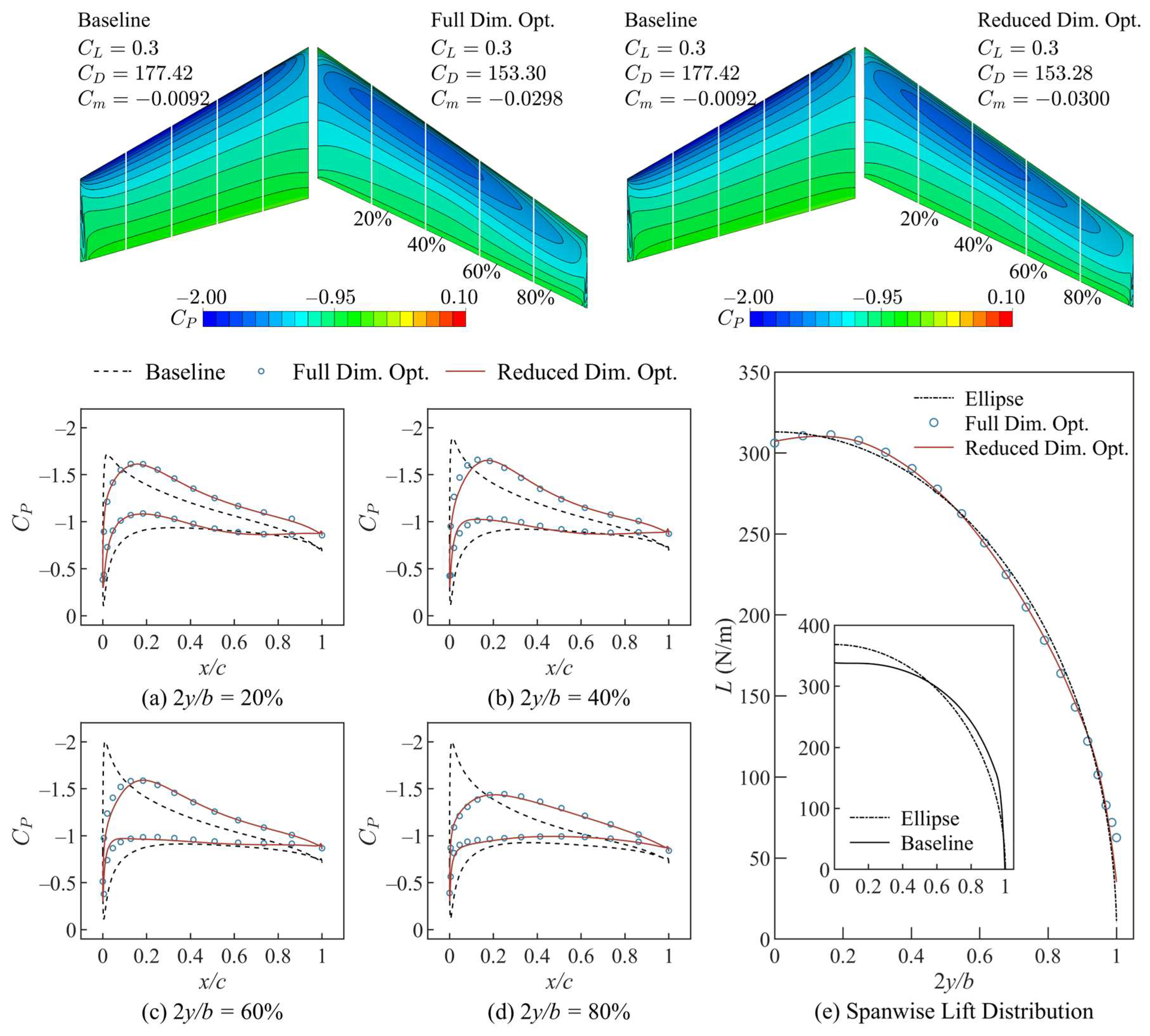
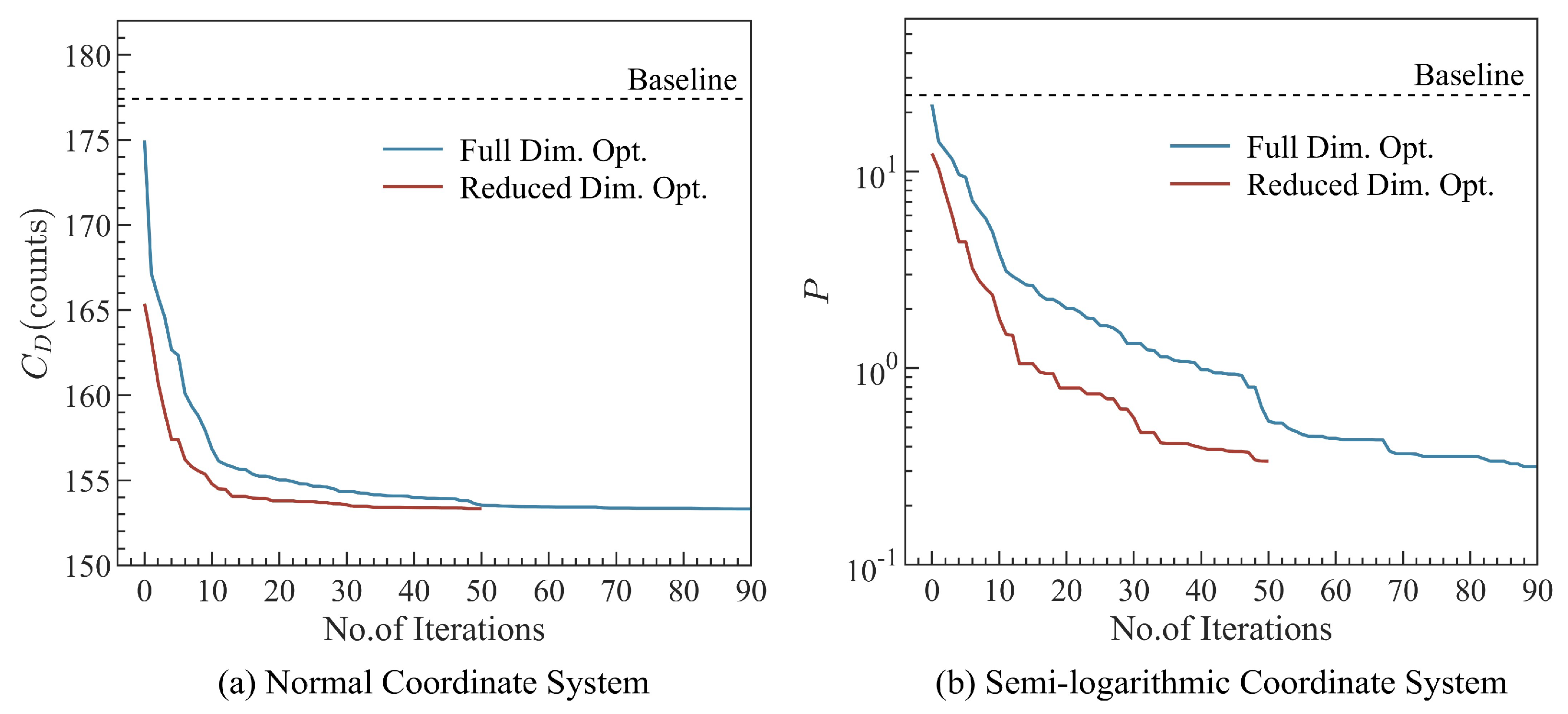
Figure 24 sketches the convergence history of 2 types of optimizations. Compared with the baseline, the optimized C D is reduced by 13.59% (177.42 to 153.30 counts) in full-dimension optimization and 13.61% (177.42 to 153.28 counts) in reduced-dimension optimization, and other variables strictly meet the constraints. Compared with full-dimensional optimization, reduced-dimensional optimization starts from a lower initial value and converges faster.
Figure 25 compares the planform, pressure distributions, and spanwise lift distributions of the baseline wing and the optimal wing. Compared with the baseline, the suction peak on the upper surface shifts backward, therefore expanding the region of the favorable pressure gradient. In addition, the spanwise lift distributions of optimal wings are closer to the elliptical distribution. Compared with full-dimensional optimization, the reduced-dimension optimization result has the same planform and similar pressure distribution. Our analysis reveals that the difference in pressure distribution is attributable to the optimization’s randomness.
Please note that the optimal planform presented is constrained by the limitations specified. The value of C m after optimization is greater than the baseline because the constraint value of C m is set to 0.03 to expand the feasible region to verify further the effectiveness of the improved approach and the surrogate-based optimization algorithm.
Furthermore, in order to eliminate the effect of randomness, each type of optimization is repeated 3 times. Figure 26 shows the average convergence history of 2 types of optimizations in normal and semi-logarithmic coordinates (where P = C D 153 ). The reduced-dimensional optimization with the improved approach significantly improves the convergence speed while maintaining global convergence. More detailed optimization results are listed in Table 4. On average, reduced-dimensional optimization is 43% quicker than full-dimensional optimization. As the number of wing sections increases, the number of dimensions that can be reduced increases, and the optimization speeds up further. Judging from the prediction accuracy of the surrogate model at the optimal value, the surrogate model is accurate enough for the engineering designer.
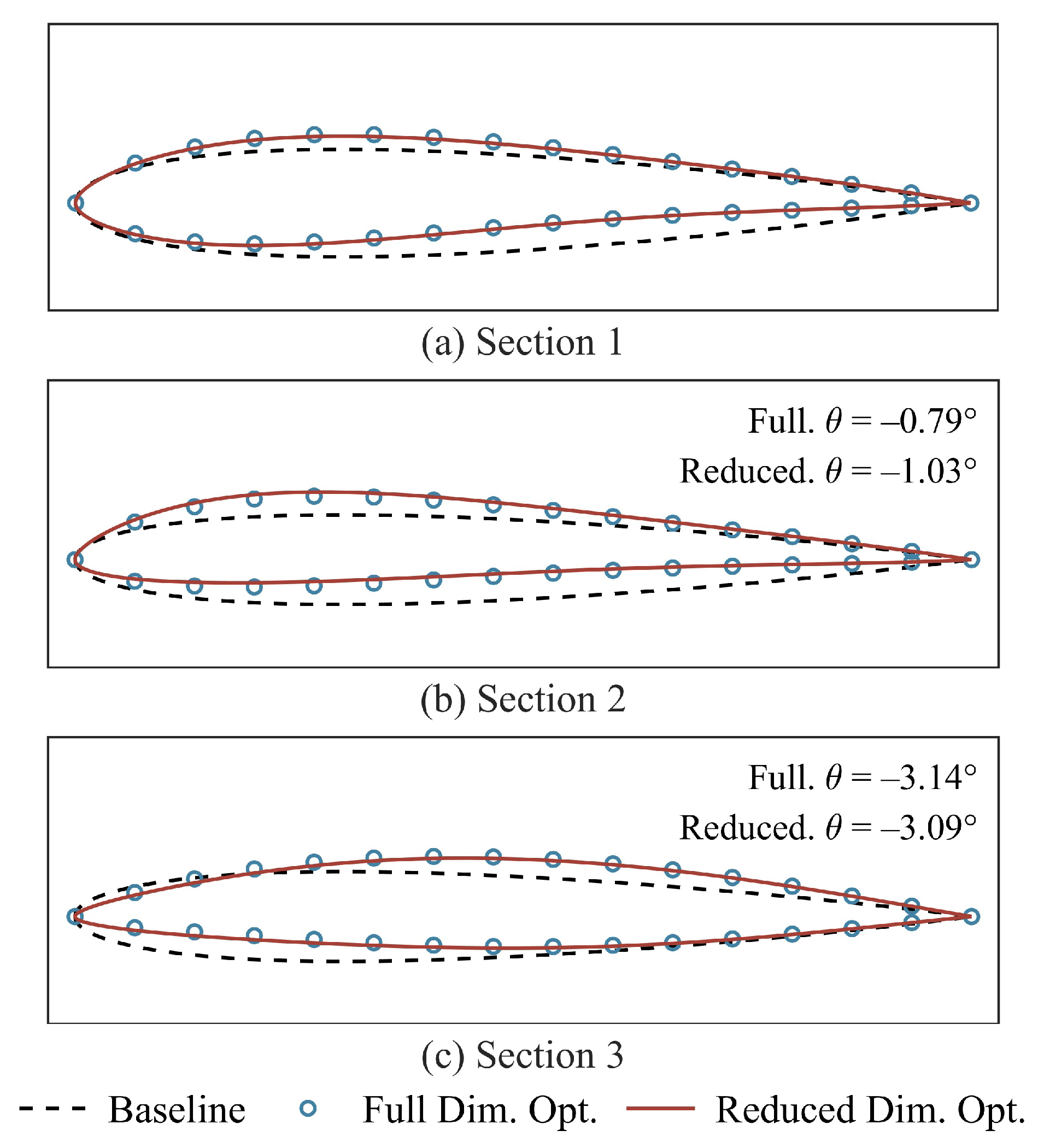
The details of the wing planform are listed in Table 5. Figure 27 depicts the average geometric shapes of wing sections of repeated 3 runs during optimizations. Compared with these results of full-dimensional and reduced-dimensional optimization, the wing planform is the same, and each section’s average shape and twist angle are highly similar.
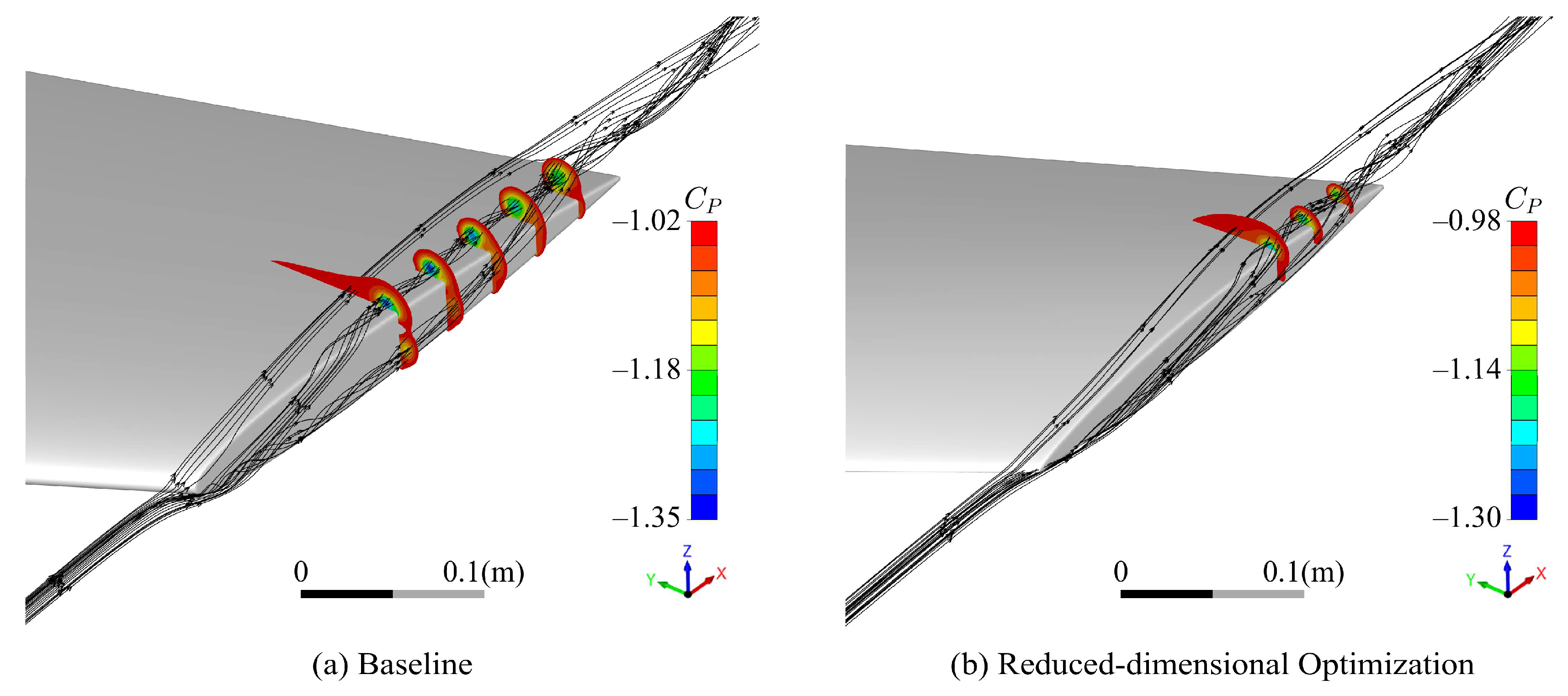
Please note the optimized shape of the wing in Section 3 in Figure 27, where the leading edge is sharp because of lower ρ 0 and large X T . The airflow is slightly separated as it passes over the wingtip of the baseline because the wingtip is not modified to make a smooth transition. The optimized shape reduces the flow separation area at the wingtips, as shown in Figure 28. However, this shape will lead to a sharp increase in the suction peak at the leading edge as the angle of attack increases. The increase in the adverse pressure gradient on the upper surface will lead to flows separating at the leading edge more easily. This issue can be improved by adding constraints on X T and ρ 0 in the optimization and modifying the wingtip.
The values of T , ρ 0 , β T E of 2 types of optimizations are listed in Table 6. It is evident that the values determined through the improved approach before optimization are identical to those acquired by full-dimensional optimization. This reverse verifies the correctness of the relationship between thickness variables ( T , ρ 0 , β T E ) and the objective function C D described in Section 4.2.

6. Conclusions

From the perspective of reducing dimensions based on aerodynamic characteristics, aiming to address the shortcomings of the traditional method based on camber-thickness decoupling, this paper proposed an improved approach to reduce dimensions to accelerate the wing aerodynamic optimization process at cruise conditions. The improved approach was derived through the analysis of the traditional method, the decoupling analysis of thickness variables, and the establishment of a data-driven aerodynamic characteristics model. The surrogate-based aerodynamic optimization of an ONERA-M6 wing in subsonic flow verified the effectiveness of the proposed improved approach. The following conclusions are drawn:
  • In the design space encompassing about 95% of the Profili airfoil library, camber and thickness variables in the objective function C D are strongly coupled. As the design space is drastically reduced to 40%, decoupling can be achieved gradually. The constraint function C m is determined primarily by the wing planform and camber variables.
  • For each configuration with varied planform and camber variables in a particular V , C L , and design space, thickness variables ( X T ,   T , ρ 0 ,   β T E ) in the objective function C D can be decoupled separately, while the influence of thickness variables in the constraint function C m is kept to a tiny order of 10 3 (longitudinal static stability margin is 3.5%).
  • With the conclusions in (1) (2) and the data-driven aerodynamic characteristics model, it is possible to first identify certain thickness variables ( T ,   ρ 0 ,   β T E ) according to the minimization based on the structural requirements. The dimension reduction amounts to 3 n (where n represents the number of wing sections). As the number of wing sections increases, the effect of dimension reduction becomes more pronounced.
  • In the aerodynamic optimization of an ONERA-M6 wing, the reduced-dimensional optimization (21-dimensional) utilizing the improved approach and the full-dimensional optimization (30-dimensional) have a consistent optimization effect (compared with the baseline, C D is reduced by about 13.6%). The results have a uniform planform and highly similar average shape of wing sections. The application of the improved approach accelerates the optimization process by an average of 43%. The values of T ,   ρ 0 ,   β T E determined by the improved approach are consistent with the results of full-dimensional optimization, which proves the accuracy of the aerodynamic characteristics model in reverse.
Overall, we proposed an improved approach on the premise that the airfoil parameterization method has a robust physical meaning (e.g., IGP, PARSEC). Unfortunately, this approach is not applicable to transonic aerodynamic optimization. Moreover, other commonly used airfoil parameterization methods (e.g., CST) have no apparent physical meaning but have strong local geometric modification capability. Since subsonic aerodynamic optimization is a typical multi-extreme problem, we will attempt to transform this paper’s findings into optimization constraints to accelerate optimization by reducing the feasible domain in the future.

Author Contributions

Conceptualization, B.J.; Methodology, B.J. and X.L.; Software, B.J.; Validation, B.J., Y.W. and J.L.; Formal analysis, B.J.; Investigation, B.J.; Resources, J.H.; Data curation, B.J.; Writing – Original Draft Preparation, B.J.; Writing – Review & Editing, B.J., J.H., X.L., Y.W., and J.L. Visualization, B.J.; Supervision, J.H.; Project Administration, J.H.; Funding Acquisition, J.H.; All authors have read and agreed to the published version of the manuscript.

Funding

This research received no external funding.

Data Availability Statement

Data are contained within the article.

Conflicts of Interest

The authors declare no conflict of interest.

Nomenclature

α angle of attack
b wingspan
b X C camber line curvature on the location of maximum camber
C maximum camber
C A a variable set composed of all variables that describe sections’ camber
C G center of gravity
C D drag coefficient
C L lift coefficient
C L , L / D m a x lift coefficient at maximum lift-to-drag ratio
C m pitch moment coefficient
C p pressure coefficient
K n longitudinal static stability margin
L chord length
L / D lift-drag ratio
M a Mach number
  S sensitivity indices, indicates the effect of design variables on the function
S w wing area
  T maximum thickness
T H a variable set composed of all variables that describe sections’ thickness
V velocity
W P a variable set composed of all variables that describe the wing planform
X C chordwise location of the maximum camber
X T chordwise location of the maximum thickness
α T E the angle between the camber line and the chord line on the trailing edge
β T E dimensionless quantity of the trailing edge boat-tail angle
Γ dihedral angle
Λ leading-edge sweep angle
ρ 0 dimensionless quantity of the leading-edge radius
θ twist angle

References

  1. Jameson, A.; Vassberg, J. Computational Fluid Dynamics for Aerodynamic Design—Its Current and Future Impact. In Proceedings of the 39th Aerospace Sciences Meeting and Exhibit, Reno, NV, USA, 8 January 2001. [Google Scholar] [CrossRef]
  2. Slotnick, J.; Khodadoust, A.; Alonso, J. CFD Vision 2030 Study: A Path to Revolutionary Computational Aerosciences; NASA/CR-2014-218178; NASA: Washington, DC, USA, 2014. [Google Scholar]
  3. Han, Z.H.; Xu, C.Z.; Qiao, J.L. Recent progress of efficient global aerodynamic shape optimization using surrogate-based approach. Acta Aeronaut. Astronaut. Sin. 2020, 41, 25–65. (In Chinese) [Google Scholar] [CrossRef]
  4. Jameson, A. Aerodynamic design via control theory. J. Sci. Comput. 1988, 3, 233–260. [Google Scholar] [CrossRef]
  5. Jameson, A. Optimum Aerodynamic Design Using CFD and Control Theory. In Proceedings of the 12th Computational Fluid Dynamics Conference, San Diego, CA, USA, 19 June 1995. [Google Scholar] [CrossRef]
  6. Kenway, G.K.W.; Mader, C.A.; He, P. Effective Adjoint Approaches for Computational Fluid Dynamics. Prog. Aerosp. Sci. 2019, 110, 100542. [Google Scholar] [CrossRef]
  7. Lyu, Z.; Martins, J.R.R.A. Aerodynamic Design Optimization Studies of a Blended-Wing-Body Aircraft. J. Aircr. 2014, 51, 1604–1617. [Google Scholar] [CrossRef]
  8. Lyu, Z.; Kenway, G.K.W.; Martins, J.R.R.A. Aerodynamic Shape Optimization Investigations of the Common Research Model Wing Benchmark. AIAA J. 2015, 53, 968–985. [Google Scholar] [CrossRef]
  9. He, X.; Li, J.; Mader, C.A. Robust Aerodynamic Shape Optimization—From a Circle to an Airfoil. Aerosp. Sci. Technol. 2019, 87, 48–61. [Google Scholar] [CrossRef]
  10. Giannakoglou, K.C. Design of Optimal Aerodynamic Shapes Using Stochastic Optimization Methods and Computational Intelligence. Prog. Aerosp. Sci. 2002, 38, 43–76. [Google Scholar] [CrossRef]
  11. Schmit, L., Jr.; Farshi, B. Some Approximation Concepts for Structural Synthesis. In Proceedings of the 14th Structures, Structural Dynamics, and Materials Conference, Williamsburg, VA, USA, 20 March 1973. [Google Scholar] [CrossRef]
  12. Simpson, T.W.; Poplinski, J.D.; Koch, P.N. Metamodels for Computer-Based Engineering Design: Survey and Recommendations. Eng. Comput. 2001, 17, 129–150. [Google Scholar] [CrossRef]
  13. Simpson, T.W.; Booker, A.J.; Ghosh, D. Approximation Methods in Multidisciplinary Analysis and Optimization: A Panel Discussion. Struct. Multidiscipl. Optim. 2004, 27, 302–313. [Google Scholar] [CrossRef]
  14. Viana, F.A.C.; Simpson, T.W.; Balabanov, V. Special Section on Multidisciplinary Design Optimization: Metamodeling in Multidisciplinary Design Optimization: How Far Have We Really Come? AIAA J. 2014, 52, 670–690. [Google Scholar] [CrossRef]
  15. Liu, J.; Han, Z.; Song, W. Comparison of infill sampling criteria in kriging-based aerodynamic optimization. In Proceedings of the 28th Congress of the International Council of the Aeronautical Sciences, Brisbane, Australia, 23–28 September 2012. [Google Scholar] [CrossRef]
  16. Parr, J.M.; Keane, A.J.; Forrester, A.I.J. Infill Sampling Criteria for Surrogate-Based Optimization with Constraint Handling. Eng. Optim. 2012, 44, 1147–1166. [Google Scholar] [CrossRef]
  17. Cox, D.D.; John, S. A Statistical Method for Global Optimization. In Proceedings of the 1992 IEEE International Conference on Systems, Man, and Cybernetics, Chicago, IL, USA, 18–21 October 1992. [Google Scholar] [CrossRef]
  18. Jones, D.R.; Schonlau, M.; Welch, W.J. Efficient global optimization of expensive black-box functions. J. Glob. Optim. 1998, 13, 455–492. [Google Scholar] [CrossRef]
  19. Han, Z.H. Research progress on Kriging model and proxy optimization algorithm. J. Aeronaut. Astronaut. 2016, 37, 3197–3225. (In Chinese) [Google Scholar] [CrossRef]
  20. Liu, F.; Han, Z.H.; Zhang, Y. Surrogate-Based Aerodynamic Shape Optimization of Hypersonic Flows Considering Transonic Performance. Aerosp. Sci. Technol. 2019, 93, 105345. [Google Scholar] [CrossRef]
  21. Liu, B.; Liang, H.; Han, Z.H. Surrogate-based aerodynamic shape optimization of a morphing wing considering a wide Mach-number range. Aerosp. Sci. Technol. 2022, 124, 107557. [Google Scholar] [CrossRef]
  22. Forrester, A.I.J.; Keane, A.J.; Bressloff, N.W. Design and Analysis of “Noisy” Computer Experiments. AIAA J. 2006, 44, 2331–2339. [Google Scholar] [CrossRef]
  23. Forrester, A.I.J.; Keane, A.J. Recent advances in surrogate-based optimization. Prog. Aerosp. Sci. 2009, 45, 50–79. [Google Scholar] [CrossRef]
  24. Shan, S.; Wang, G.G. Survey of Modeling and Optimization Strategies to Solve High-Dimensional Design Problems with Computationally-Expensive Black-Box Functions. Struct. Multidiscipl. Optim. 2010, 41, 219–241. [Google Scholar] [CrossRef]
  25. Han, Z.H.; Görtz, S. Hierarchical kriging model for variable-fidelity surrogate modeling. AIAA J. 2012, 50, 1885–1896. [Google Scholar] [CrossRef]
  26. Park, C.; Haftka, R.T.; Kim, N.H. Remarks on Multi-Fidelity Surrogates. Struct. Multidiscipl. Optim. 2017, 55, 1029–1050. [Google Scholar] [CrossRef]
  27. Giselle Fernández-Godino, M.; Park, C.; Kim, N.H. Issues in deciding whether to use multifidelity surrogates. AIAA J. 2019, 57, 2039–2054. [Google Scholar] [CrossRef]
  28. Brevault, L.; Balesdent, M.; Hebbal, A. Overview of Gaussian process based multi-fidelity techniques with variable relationship between fidelities, application to aerospace systems. Aerosp. Sci. Technol. 2020, 107, 106339. [Google Scholar] [CrossRef]
  29. Han, Z.H.; Xu, C.Z.; Zhang, L. Efficient aerodynamic shape optimization using variable-fidelity surrogate models and multilevel computational grids. Chin. J. Aeronaut. 2020, 33, 31–47. [Google Scholar] [CrossRef]
  30. Dwight, R.; Han, Z.H. Efficient Uncertainty Quantification Using Gradient-Enhanced Kriging. In Proceedings of the 50th AIAA/ASME/ASCE/AHS/ASC Structures, Structural Dynamics, and Materials Conference, Palm Springs, CA, USA, 4 May 2009. [Google Scholar] [CrossRef]
  31. Han, Z.H.; Görtz, S.; Zimmermann, R. Improving variable-fidelity surrogate modeling via gradient-enhanced kriging and a generalized hybrid bridge function. Aerosp. Sci. Technol. 2013, 25, 177–189. [Google Scholar] [CrossRef]
  32. Song, C.; Song, W.; Yang, X. Gradient-enhanced hierarchical kriging model for aerodynamic design optimization. J. Aerosp. Eng. 2017, 30, 04017072. [Google Scholar] [CrossRef]
  33. Han, Z.H.; Zhang, Y.; Song, C.X. Weighted gradient-enhanced kriging for high-dimensional surrogate modeling and design optimization. AIAA J. 2017, 55, 4330–4346. [Google Scholar] [CrossRef]
  34. Sóbester, A.; Leary, S.J.; Keane, A.J. A parallel updating scheme for approximating and optimizing high fidelity computer simulations. Struct. Multidiscipl. Optim. 2004, 27, 371–383. [Google Scholar] [CrossRef]
  35. Liu, J.; Song, W.P. Efficient aerodynamic shape optimization of transonic wings using a parallel infilling strategy and surrogate models. Struct. Multidiscipl. Optim. 2017, 55, 925–943. [Google Scholar] [CrossRef]
  36. Wang, Y.; Han, Z.H.; Zhang, Y. Efficient Global Optimization Using Multiple Infill Sampling Criteria and Surrogate Models. In Proceedings of the 2018 AIAA Aerospace Sciences Meeting, Kissimmee, FL, USA, 8 January 2018. [Google Scholar] [CrossRef]
  37. Painchaud-Ouellet, S.; Tribes, C.; Trépanier, J.Y. Airfoil shape optimization using a nonuniform rational b-splines parametrization under thickness constraint. AIAA J. 2006, 44, 2170–2178. [Google Scholar] [CrossRef]
  38. Song, W.; Keane, A.J. Surrogate-based aerodynamic shape optimization of a civil aircraft engine nacelle. AIAA J. 2007, 45, 2565–2574. [Google Scholar] [CrossRef]
  39. Van Der Maaten, L.; Postma, E.; Van den Herik, J. Dimensionality reduction: A comparative. J. Mach. Learn. Res. 2009, 10, 13. [Google Scholar]
  40. Ghisu, T.; Parks, G.; Jarrett, J.; Clarkson, P. Accelerating Design Optimization Via Principal Components Analysis. In Proceedings of the 12th AIAA/ISSMO Multidisciplinary Analysis and Optimization Conference, Victoria, BC, Canada, 10 September 2008. [Google Scholar] [CrossRef]
  41. Toal, D.J.J.; Bressloff, N.W.; Keane, A.J.; Holden, C.M.E. Geometric filtration using proper orthogonal decomposition for aerodynamic design optimization. AIAA J. 2010, 48, 916–928. [Google Scholar] [CrossRef]
  42. Ghoman, S.; Wang, Z.; Chen, P.; Kapania, R. A POD-Based Reduced Order Design Scheme for Shape Optimization of Air Vehicles. In Proceedings of the 53rd AIAA/ASME/ASCE/AHS/ASC Structures, Structural Dynamics and Materials Conference, Honolulu, HI, USA, 23 April 2012. [Google Scholar]
  43. Ghoman, S.S.; Wang, Z.; Chen, P.C. Hybrid optimization framework with proper-orthogonal-decomposition-based order reduction and design-space evolution scheme. J. Aircr. 2013, 50, 1776–1786. [Google Scholar] [CrossRef]
  44. Viswanath, A.; Forrester, A.I.J.; Keane, A.J. Dimension reduction for aerodynamic design optimization. AIAA J. 2011, 49, 1256–1266. [Google Scholar] [CrossRef]
  45. Lukaczyk, T.W.; Constantine, P.; Palacios, F. Active Subspaces for Shape Optimization. In Proceedings of the 10th AIAA Multidisciplinary Design Optimization Conference, National Harbor, MD, USA, 13 January 2014. [Google Scholar] [CrossRef]
  46. Abbott, I.H.; Von Doenhoff, A.E. Theory of Wing Sections: Including a Summary of Airfoil Data; Dover Publications Inc.: New York, NY, USA, 1959; pp. 65–66. [Google Scholar]
  47. Berkenstock, D.; Alonso, J.J.; Lessard, L. A Convex Optimization Approach to Thin Airfoil Design. In Proceedings of the 2022 AIAA Aviation and Aeronautics Forum and Exposition, Chicago, IL, USA, 1 July 2022. [Google Scholar] [CrossRef]
  48. Wei, C.; Huang, J.; Song, L. Study on a Rapid Aerodynamic Optimization Method of Flying Wing Aircraft for Conceptual Design. Int. J. Aerosp. Eng. 2022, 2022, 5775355. [Google Scholar] [CrossRef]
  49. Lu, X.; Huang, J.; Song, L. An Improved Geometric Parameter Airfoil Parameterization Method. Aerosp. Sci. Technol. 2018, 78, 241–247. [Google Scholar] [CrossRef]
  50. Spalart, P.; Allmaras, S. A One-Equation Turbulence Model for Aerodynamic Flows. In Proceedings of the 30th Aerospace Sciences Meeting and Exhibit, Reno, NV, USA, 6 January 1992. [Google Scholar]
  51. Schmitt, V.; Charpin, F. Pressure Distributions on the ONERA-M6-Wing at Transonic Mach Numbers, Experimental Data Base for Computer Program Assessment; AGARD AR-138; NATO: Brussels, Belgium, 1979. [Google Scholar]
  52. Wolhart, W.D.; Thomas, D.F., Jr. Static Longitudinal and Lateral Stability Characteristics at Low Speed of Unswept-Midwing Models Having Wings with an Aspect Ratio of 2, 4, or 6; NACA-TN-4077; NASA: Washington, DC, USA, 1957. [Google Scholar]
  53. Saltelli, A.; Sobol, I.M. About the use of rank transformation in sensitivity analysis of model output. Reliab. Eng. Syst. Saf. 1995, 50, 225–239. [Google Scholar] [CrossRef]
  54. Sobol, I.M. Global sensitivity indices for nonlinear mathematical models and their Monte Carlo estimates. Math. Comput. Simul. 2001, 55, 271–280. [Google Scholar] [CrossRef]
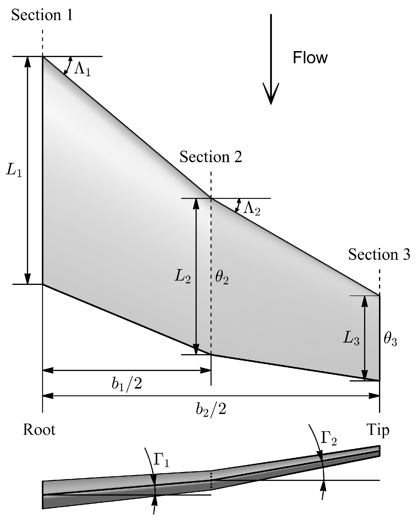
Figure 1. Parametric modeling of wing planform.
Aerospace 11 00080 g001
Figure 2. Parameters describing the wing section by the IGP method.
Aerospace 11 00080 g002
Figure 3. Histogram of airfoil fitting results by the IGP method.
Aerospace 11 00080 g003
Figure 4. The O-type structured mesh adopted in CFD simulation.
Aerospace 11 00080 g004
Figure 5. Comparison of the pressure distribution of the ONERA-M6 wing between CFD and experiments ( M a = 0.84 , R e = 1.17 × 10 7 , α = 3.06 ° ).
Aerospace 11 00080 g005
Figure 6. Comparison of the aerodynamic performance of the clean wing between CFD and experiments ( M a = 0.13 , R e = 1 × 10 6 ).
Aerospace 11 00080 g006
Figure 7. Flowchart of the surrogate-based optimization algorithm with a parallel infilling strategy and CFD.
Aerospace 11 00080 g007
Figure 8. Schematics of 15 samples selected by LHS and Optimal-LHS for a two-dimensional problem.
Aerospace 11 00080 g008
Figure 9. Convergence history of optimizing a G9 function.
Aerospace 11 00080 g009
Figure 10. Convergence history of optimizing a Sum-Squares function.
Aerospace 11 00080 g010
Figure 11. Comparison of theoretical and calculated values of sensitivity of a benchmark function.
Aerospace 11 00080 g011
Figure 12. Wing planforms of DLR-F4, ONERA-M6, and a typical flying wing.
Aerospace 11 00080 g012
Figure 13. The main and interaction effect of camber and thickness variables in C D , C m within a wide-range design space, which contains 95% Profili airfoil library (the inner ring pie chart represents C D , and the outer pie chart represents C m ).
Aerospace 11 00080 g013
Figure 14. The main and interaction effect of camber and thickness variables in C D , C m within a low-range design space, which contains 40% Profili airfoil library (the inner ring pie chart represents C D , and the outer pie chart represents C m ).
Aerospace 11 00080 g014
Figure 15. Design variables for wing planform used to generate wing camber surfaces.
Aerospace 11 00080 g015
Figure 16. Coupling sensitivity indices of thickness variables of all configurations.
Aerospace 11 00080 g016
Figure 17. The standard deviation of the influence of thickness variables on C m of all configurations (longitudinal static stability margin is 3.5%).
Aerospace 11 00080 g017
Figure 18. Relationship between thickness variables and C D of configuration 1 at 0.147 M a .
Aerospace 11 00080 g018
Figure 19. Relationship between thickness variables and C D of all configurations at 0.147 M a (See Figure 18 for the chart format).
Aerospace 11 00080 g019
Figure 20. Relationship between thickness variables and C D of all configurations at 0.3 M a (See Figure 18 for the chart format).
Aerospace 11 00080 g020
Figure 21. Relationship between thickness variables and C D of all configurations at 0.6 M a (See Figure 18 for the chart format).
Aerospace 11 00080 g021
Figure 22. Correlation indexes between thickness variables and C D of all configurations.
Aerospace 11 00080 g022
Figure 23. Parameterization of an ONERA-M6 wing with 3 sections.
Aerospace 11 00080 g023
Figure 24. Comparison of convergence history of full-dimension and reduce-dimension optimization.
Aerospace 11 00080 g024
Figure 25. Comparison of planform, pressure distributions, and spanwise lift distributions of baseline and optimal wings.
Aerospace 11 00080 g025
Figure 26. The average convergence history of repeated 3 runs during optimizations.
Aerospace 11 00080 g026
Figure 27. Average geometric shapes of wing sections of optimal wings of repeated 3 runs during optimizations.
Aerospace 11 00080 g027
Figure 28. Comparison of pressure coefficient contour of the wing tip.
Aerospace 11 00080 g028
Table 1. Range of values for design variables.
BaselineLower LimitUpper LimitRange
L 1 805.9644.7967.1±20%
L 3 453.3362.6544.0±20%
b 2 / 2 1196.3837.41555.2±30%
Λ 1 , Λ 2 30045/
θ 2 0−42/
θ 3 0−82/
Γ 1 , Γ 2 0−1515/
Section 1,2,3/IGP (4 camber parameters)
Note: L 2 = L 1 + L 3 / 2 , b 1 = b 2 / 2 , Length in mm, Angle in degree.
Table 2. The flow conditions and the number of samples in which flow separation occurred.
ConfigurationFlow ConditionsNumber of Samples
(Existent Flow Separation)
1 V = 0.6 M a C L = 0.75 C L , ( L / D ) m a x 0
C L = C L , ( L / D ) m a x 17
3 V = 0.6 M a C L = 0.75 C L , ( L / D ) m a x 0
C L = C L , ( L / D ) m a x 13
8 V = 0.6 M a C L = 0.75 C L , ( L / D ) m a x 21
C L = C L , ( L / D ) m a x 1
Table 3. Range of values for design variables.
BaselineFull-Dimensional
(30 Variables)
Reduced-Dimensional
(21 Variables)
L 1 805.9[0.85, 1.15] · BaselineSame as
Full-dimensional
L 3 453.3[0.85, 1.15] · Baseline
b / 2 1196.3[0.85, 1.15] · Baseline
Λ 1 30[−5, 5] + Baseline
θ 2 0[−4, 2]
θ 3 0[−8, 2]
Section 1NACA 0012IGP
8 parameters
IGP
5 parameters
( X C , C , b X C , α T E , X T )
Section 2NACA 0008
Section 3NACA 0008
Note: Length in mm, Angle in degree.
Table 4. Results of repeated 3 runs during optimizations.
No.Number
of CFD
Evaluations
Total Time Cost
(h)
Average
Time Saved
(%)
Optimal Results Reduction   of C D
(%)
Prediction   Error   of   C D
at Optimum
(%)
C L C D
(Counts)
C m
Baseline 0.3177.42−0.0092
Full-
dimensional
160 + 36045.5 0.3153.34−0.030013.570.024
260 + 36045.6 0.3153.30−0.029813.590.024
360 + 36045.3 0.3153.31−0.029913.590.020
Reduced-
dimensional
160 + 20025.842.960.3153.37−0.029913.560.016
260 + 20026.20.3153.37−0.029913.560.002
360 + 20025.80.3153.28−0.030013.610.013
Note: Each CFD evaluation consists of 4 Angle of attack state evaluations.
Table 5. Results of wing planform of repeated 3 runs during optimizations.
No. L 1 L 3 b / 2 Λ 1 Δ S w
Baseline 805.9453.31196.330
Full-
dimensional
Both in
1,2,3 runs
685.0385.31375.735−2.25%
Reduced-
dimensional
Both in
1,2,3 runs
685.0385.31375.735−2.25%
Note: Length in mm, Angle in degree.
Table 6. Results of T * , ρ 0 * , β T E * of repeated 3 runs during optimizations.
No. T 1 ,   T 2 ,   T 3 ρ 0.1 ,   ρ 0.2 ,   ρ 0.3 β T E , 1 ,   β T E , 2 ,   β T E , 3
Full-
dimensional
Both in
1,2,3 runs
0.12, 0.10, 0.100.16, 0.16, 0.161.50, 1.50, 1.50
(Determine by optimization)
Reduced-
dimensional
Both in
1,2,3 runs
0.12, 0.10, 0.100.16, 0.16, 0.161.50, 1.50, 1.50
(Determine by the improved approach)
Disclaimer/Publisher’s Note: The statements, opinions and data contained in all publications are solely those of the individual author(s) and contributor(s) and not of MDPI and/or the editor(s). MDPI and/or the editor(s) disclaim responsibility for any injury to people or property resulting from any ideas, methods, instructions or products referred to in the content.