Multi-Phase Vertical Take-Off and Landing Trajectory Optimization with Feasible Initial Guesses

Abstract

The advancement of electric vertical take-off and landing (eVTOL) aircraft has expanded the horizon of urban air mobility. However, the challenge of generating precise vertical take-off and landing (VTOL) trajectories that comply with airworthiness requirements remains. This paper presents an approach for optimizing VTOL trajectories considering six degrees of freedom (6DOF) dynamics and operational constraints. Multi-phase optimal control problems are formulated to address specific constraints in various flight stages. The incremental nonlinear dynamic inversion (INDI) controller is employed to execute the flight mission in each phase. Controlled flight simulations yield dynamically feasible trajectories that serve as initial guesses for generating sub-optimal trajectories within individual phases. A feasible and sub-optimal initial guess for the holistic multi-phase problem is established by concatenating these single-phase trajectories. Focusing on a tilt-wing eVTOL aircraft, this paper computes VTOL trajectories leveraging the proposed initial guess generation procedure. These trajectories account for complex flight dynamics, align with various operation constraints, and minimize electric energy consumption.

1. Introduction

Recent advancements in electric propulsion technology have promoted the development of electric vertical take-off and landing (eVTOL) aircraft. These vehicles use distributed electric propulsion systems to achieve VTOL capabilities. Many eVTOL aircraft can generate aerodynamic lift in forward flight, reducing electric energy consumption. These features allow eVTOL aircraft to operate flexibly and efficiently in urban airspace, making them promising for Urban Air Mobility (UAM).

In low-altitude airspace, eVTOL aircraft face a heightened risk of conflict with ground structures and obstacles, necessitating detailed flight planning for take-off and landing. Boeing and Wisk have proposed using trajectory-based flight plans for eVTOL air traffic management [1]. Predictable flight plans enable timely separation and sequencing at vertiports. Additionally, future eVTOL aircraft may not require a pilot but instead rely on automatic flight to reduce weight. In this context, precise flight trajectories are imperative for safe and efficient autonomous operations. Due to limited onboard computing capabilities, these trajectories are generally computed offline. Moreover, eVTOL aircraft typically possess limited energy storage but require high power during take-off and landing. Therefore, low-energy consumption take-off and landing trajectories are crucial for the economical and sustainable operations of eVTOL aircraft.

Recognizing the criticality of the take-off and landing phases, certification agencies have initiated the development of relevant requirements for VTOL aircraft. The European Aviation Safety Agency (EASA) has issued the Special Condition for small-category VTOL aircraft (SC-VTOL) [2] and the Means of Compliance (MOC SC-VTOL) [3]. EASA has also released technical specifications for vertiports [4]. The Civil Aviation Administration of China (CAAC) has released special conditions for the EH-216-S model [5]. Meanwhile, the Federal Aviation Administration (FAA) has published airworthiness standards for Joby JAS4-1 and Archer M001 models [6,7] and released a guidance on vertiport design [8]. These regulations pose requirements on flight path geometry and performance along the trajectory. In addition to airworthiness requirements, the inherent complexities of eVTOL flight dynamics must be considered when planning trajectories. More than simple point-mass models are required to capture the intricate characteristics of eVTOL aircraft. Moreover, aircraft attitude or rotational motion constraints may arise in VTOL operations, requiring comprehensive six degrees of freedom (6DOF) dynamics models.

Several studies addressed optimal flight trajectories for eVTOL aircraft. Many employed point-mass dynamic models or even simpler longitudinal motion models. For example, Wei et al. [9] calculated the minimum energy landing trajectory using EH-184’s longitudinal model. Chauhan et al. [10] calculated the minimum energy take-off trajectory of a tilt-wing eVTOL using a 2DOF longitudinal model. Other similar studies also utilized simplified dynamic models [11,12]. Yet, only a handful of studies have undertaken trajectory optimization for VTOL aircraft based on 6DOF models [13,14,15]. Furthermore, only a few studies have considered airworthiness requirements for VTOL operations [15,16]. Incorporating the 6DOF dynamics of an eVTOL, which are highly coupled, nonlinear, and potentially unstable, poses a challenging large-scale trajectory optimization problem [17]. When airworthiness requirements are factored in, various constraints across multiple flight phases increase the difficulty of achieving a converged solution using gradient-based solvers.

In the context of solving such complex trajectory optimization tasks, a suitable initial guess is crucial. If the initial guess strays too far from the optimal solution, the optimization algorithm may not converge [18]. A good initial guess also aids in determining scaling factors and discretization size in the optimization problem [15]. Several methods have been proposed to address this issue. For instance, Ref. [18] introduced a hierarchical trajectory optimization algorithm that begins with a basic point-mass model and a feasible initial guess, progressively refining the model’s fidelity until the optimal trajectory for a 6DOF model is attained. Bittner et al. [19] employed an Iterated Extended Kalman Filter to generate an initial guess for a 6DOF model, leveraging the optimal trajectory from a point-mass model. These methods rely on solving the point-mass trajectory with a sound initial guess. However, the point-mass trajectory problem can be challenging for a multi-phase vertical take-off and landing task. Furthermore, as discussed earlier, the optimal trajectory based on a point-mass model may be infeasible for actual flight, rendering the initial guess for the 6DOF trajectory likewise infeasible.

This study aims to generate precise VTOL trajectories for eVTOL aircraft considering various operational constraints. Precision is assured by modeling the 6DOF flight dynamics. Multi-phase problems are formulated to address unique requirements in each flight stage. We propose a method for generating feasible initial guesses using the Incremental Nonlinear Dynamic Inversion (INDI) controller. The process begins with simple pilot commands to accomplish the mission of the first phase. The time histories of states and controls during simulation are used as the initial guess for computing a sub-optimal trajectory in this phase. Subsequently, new commands are designed to complete the mission in the next phase, and another sub-optimal trajectory is calculated. These phase-wise calculations result in sub-optimal trajectories for individual phases, which are then concatenated to provide a feasible initial guess for the entire multi-phase problem. Our primary contributions in this study are as follows:

• A comprehensive analysis of operational constraints critical to VTOL trajectory optimization, coupled with the formulation of multi-phase take-off and landing trajectories to address unique constraints in each phase of VTOL operations.
• A “divide and conquer” approach proposed to generate feasible initial guesses for multi-phase problems, effectively leveraging the INDI controller.
• Computation of high-fidelity, energy-minimum take-off and landing trajectories for a tilt-wing eVTOL aircraft, revealing its unique flight characteristics.

The remainder of this paper is organized as follows: Section 2 summarizes the operational constraints on VTOL trajectories. Section 3 elaborates on the 6DOF flight dynamics model of the eVTOL and the INDI control system. Section 4 and Section 5 present detailed procedures to generate minimum energy take-off and landing trajectories. Finally, Section 6 briefly concludes the paper.

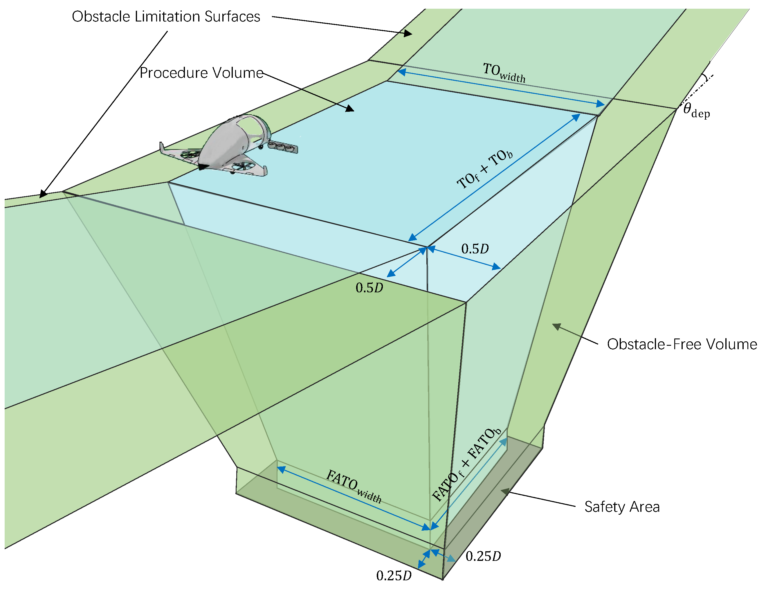
2. Operational Constraints on VTOL Trajectories

This section provides an in-depth analysis of the constraints involved in VTOL trajectory optimization. These constraints are primarily derived from three sources: airworthiness requirements, aircraft dynamics, and the specific objectives of the mission task. These constraints are hereafter referred to as “operational constraints” in this paper. The current airworthiness requirements and flight dynamics constraints are briefly overviewed here, while the specific mission task is addressed in Section 4 and Section 5.

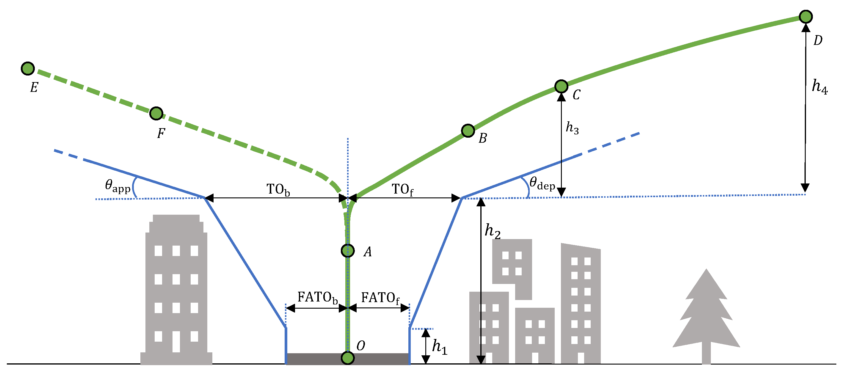
2.1. Airworthiness Requirements

EASA is establishing a new regulatory framework for eVTOL aircraft. The SC-VTOL [2] provides baseline regulations for VTOL aircraft’s take-off and landing performance, while the MOC documents offer more detailed requirements. MOC-2 [3] specifies vertical flight paths for eVTOL aircraft in urban environments, as illustrated in Figure 1. The specific requirements associated with these flight paths are interpreted and summarized in

Table 1. Requirements for the vertical take-off and landing paths in MOC-2 [3].

Nr.		Requirement
Take-off	1	The aircraft should reach $V_{\mathrm{TOSS}}$ while clearing any surface by 4.6 m
	2	$V_{\mathrm{TOSS}}$ should be reached at or before 10.7 m (35 ft) above $h_2$
	3	In the first climb segment, the minimum climb gradient is $4.5\%$ and the speed is no less than $V_{\mathrm{TOSS}}$
	4	In the second climb segment, the minimum climb gradient is 2.5%
	5	The aircraft should be accelerated to $V_{\mathrm{FTO}}$ at a height over 305 m (1000 ft)
	6	After reaching $V_{\mathrm{FTO}}$, the aircraft should be capable of a directional trajectory change with at least 3${}^{\circ }$/s and no descent
Landing	1	LDP should be reached at a speed equal or lower to the reference speed $V_{\mathrm{REF}}$
	2	The speed, position, and attitude of the aircraft when it touches the ground are within certain ranges

. Additionally, MOC-2 mandates that aircraft paths near the vertiport be confined within a “funnel-shaped” region (referred to as the Procedure Volume hereafter) to circumvent obstacles. The three-dimensional depiction of this volume is shown in Figure 2.

Table 2. Parameters of the VTOL procedure volume [3,4].

Symbol	Meaning	Range	Recommanded Value
$h_1$	Low hover height	-	3 m
$h_2$	High hover height	≥$h_1$	30.5 m
${\mathrm{TO}}_{\mathrm{width}}$	Width at $h_2$	≤$5D$	$2D$
${\mathrm{TO}}_{\mathrm{f}}$	Front distance at $h_2$	≤$5D$	$1.5D$
${\mathrm{TO}}_{\mathrm{b}}$	Back distance at $h_2$	≤$5D$	$1.5D$
${\mathrm{FATO}}_{\mathrm{width}}$	Width of the FATO	≥$1.5D$	$1.5D$
${\mathrm{FATO}}_{\mathrm{f}}$	Front distance on FATO	≥$0.75D$	$0.75D$
${\mathrm{FATO}}_{\mathrm{b}}$	Back distance on FATO	≥$0.75D$	$0.75D$
${\theta }_{\mathrm{app}}$	Slope of approach surface	≥$4.5\%$	12.5%
${\theta }_{\mathrm{dep}}$	Slope of departure surface	≥$4.5\%$	12.5%

outlines its geometric definitions and recommended dimensions. The dimension D denotes the “diameter of the smallest circle enclosing the VTOL aircraft projection on a horizontal plane, while the aircraft is in the take-off or landing configuration, with rotor(s) turning if applicable”. Furthermore, the EASA document PTS-VPT-DSN [4] elaborates on the take-off and landing procedures near the vertiport, extending the Procedure Volume to an “Obstacle-Free Volume”, as illustrated in Figure 2. This Obstacle-Free Volume features protective surfaces in the forward and backward directions. The inner edges of these surfaces are located at the height of $h_2$ with a width of ${\mathrm{TO}}_{\mathrm{width}}+D$. The outer edges extend to a height of 152 m above the Final Approach and Take-off Area (FATO).

The CAAC and FAA have also published special conditions or airworthiness standards for several eVTOL models [5,6,7]. However, these documents do not provide detailed specifications for take-off and landing trajectories. The FAA’s interim guidance for vertiport design, EB-105 [8], specifies the dimensions of a vertiport and the permissible airspace. Currently, this guidance adopts a conservative approach due to “a lack of validated data on the performance capabilities of VTOL aircraft”. Consequently, this paper primarily focuses on the airworthiness requirements for VTOL trajectories as presented in SC-VTOL MOC-2 [3] and PTS-VPT-DSN [4].

2.2. Flight Dynamics Constraints

EVTOL aircraft should adhere to various flight dynamics constraints to ensure flight safety and passenger comfort. Firstly, the aircraft must operate within an appropriate flight envelope. SC-VTOL and the EH-216-S special conditions define three flight envelope concepts: the normal flight envelope, the operational flight envelope, and the limited flight envelope. When planning VTOL trajectories, either the normal flight envelope or more conservative envelopes determined by other formal methods [20] should be considered. While current airworthiness regulations do not provide specific content regarding eVTOL flight envelopes, a reference can be found in AC 25-7D [21], Appendix E. This document provides flight envelope definitions for transport category airplanes using parameters such as airspeed, pitch angle, roll angle, altitude, normal load factor, angle of attack, and side-slip angle. At lower speeds, the angle of attack and side-slip angle can exhibit large values. Therefore, this paper includes velocity components in the body frame as part of the envelope parameters, along with flight states impacting passenger comfort, such as acceleration and aircraft attitude. Limiting the descent rate in hover is necessary to prevent the aircraft from entering a vortex ring state. Besides the envelope, physical limits on control inputs and the propulsion system, such as propeller speed, torque, power, and actuator deflection, are also considered in trajectory optimization.

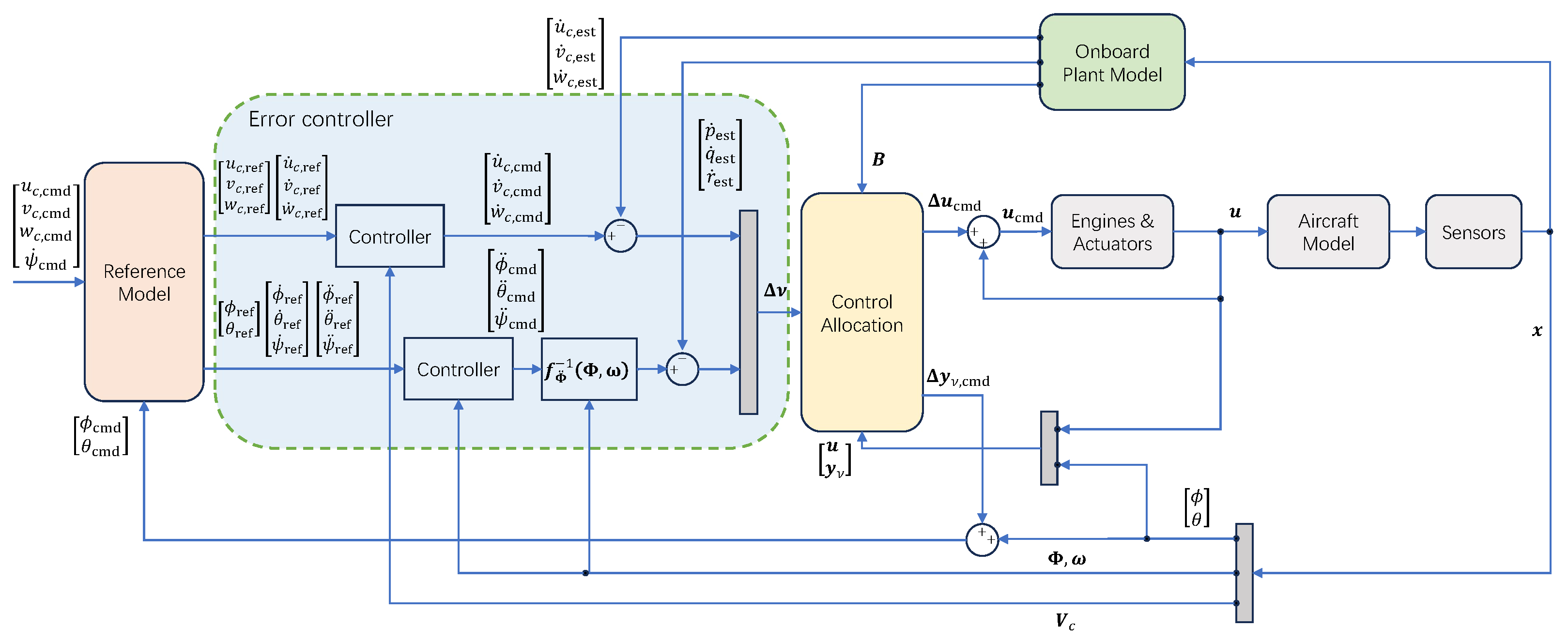
3. Six-DOF Dynamics Model and Controller

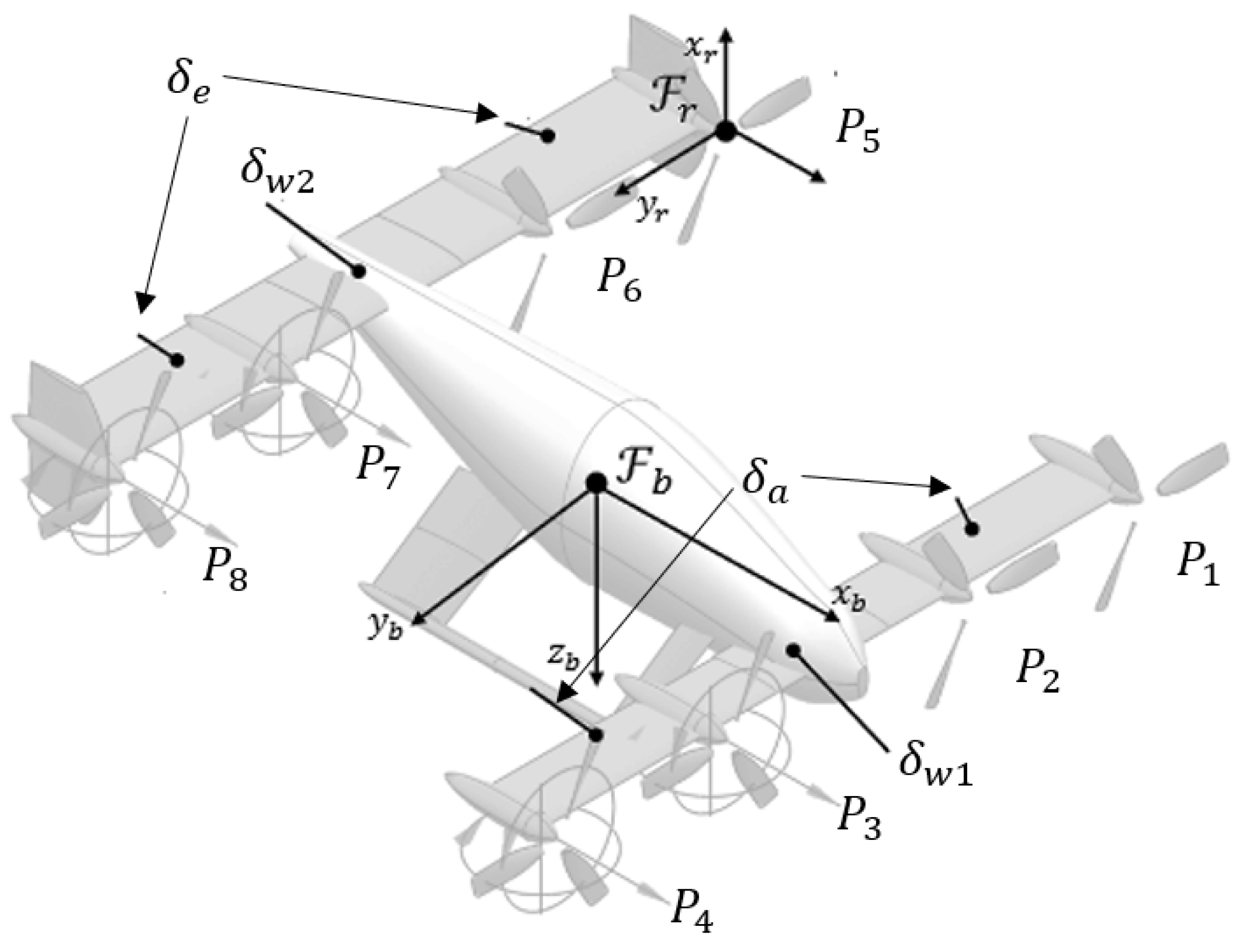
3.1. Configuration Parameters

This paper focuses on a tilt-wing eVTOL model adapted from [22]. As depicted in Figure 3, this eVTOL resembles the Airbus Vahana model, featuring front and rear tilt-wings, each equipped with four propulsion units. It also includes vertical stabilizers and multiple aerodynamic control surfaces, which provide stability and controllability during wing-borne flight. Some key parameters for this eVTOL model are listed in

Table 3. Some parameters of the example tilt-wing eVTOL aircraft.

Parameter	Value	Unit
Mass m	575	kg
Wing span b	6	m
Wing mean chord length c	0.67	m
Wing reference area $S_{\mathrm{ref}}$	8.04	${\mathrm{m}}^2$
Wing stall angle ${\alpha }_{\mathrm{s}}$	15	${}^{\circ }$
Diameter of propeller $D_P$	1.5	m
VTOL dimension D	8	m
Stall speed $V_{\mathrm{s}}$	35	m/s
Take-off safety speed $V_{\mathrm{TOSS}}$	11	m/s
Final take-off speed $V_{\mathrm{FTO}}$	46	m/s
Landing reference speed $V_{\mathrm{REF}}$	20	m/s

.

3.2. Flight Dynamics Model

Considering the low operational altitude and limited range of the eVTOL, this paper omits the effects of Earth’s curvature and rotation. A navigation coordinate system, denoted as the “N-frame” ($O-X_N{Y}_N{Z}_N$), is established to represent the aircraft’s position. The origin of this system is anchored at the parking site. The $O-X_N$ axis aligns with the centerline of the obstacle limitation surfaces, and the $O-Z_N$ axis extends vertically downward. The motion of the eVTOL is governed by the equations of rigid body dynamics formulated in the body frame (termed the “B-frame”).

$${\left({\dot{\mathit{V}}}_K^G\right)}_B^{EB}=\frac{1}{m}\sum {\left({\mathit{F}}^G\right)}_B-{\left({\mathit{\omega }}_K^{OB}\right)}_B\times {\left({\mathit{V}}_K^G\right)}_B^E$$

(1)

$${\left({\dot{\mathit{\omega }}}_K^{OB}\right)}_B={\mathit{I}}^{-1}\left[\sum {\left({\mathit{M}}^G\right)}_B-{\left({\mathit{\omega }}_K^{OB}\right)}_B\times \mathit{I}{\left({\mathit{\omega }}_K^{OB}\right)}_B\right]$$

(2)

$${\left(\dot{\mathit{R}}\right)}_{NG}^E={\mathit{M}}_{NO}{\mathit{M}}_{OB}{\left({\mathit{V}}_K^G\right)}_B^E$$

(3)

where ${\left({\mathit{V}}_K^G\right)}_B^E={[u_{\mathrm{b}},v_{\mathrm{b}},w_{\mathrm{b}}]}^T$ is the aircraft’s velocity in the B-frame, ${\left({\mathit{\omega }}_K^{OB}\right)}_B={[p,q,r]}^T$ is the angular rate of the B-frame with respect to the North-East-Down (NED) frame, ${\left(\mathit{R}\right)}_{NG}^E=$ is the position in the N-frame, $\mathit{I}$ is the inertia matrix, ${\mathit{M}}_{OB}$ and ${\mathit{M}}_{NO}$ are direction cosine matrices (DCM) from the B-frame to the NED-frame, and from the NED-frame to the N-frame, respectively.

The total force comprises gravitational, aerodynamic, and propulsive forces:

$${\left({\mathit{F}}^G\right)}_B={\mathit{M}}_{BO}\left[\begin{array}{c}0\\ 0\\ mg\end{array}\right]+{\mathit{M}}_{BA}\frac{1}{2}\rho V_{\mathrm{a}}^2{S}_{\mathrm{ref}}\left[\begin{array}{c}-C_D\\ C_S\\ -C_L\end{array}\right]+\sum _{i=1}^8{\mathit{M}}_{B{P}_i}\left[\begin{array}{c}0\\ 0\\ C_{FP}\rho {\omega }_i^2{D}_P^4\end{array}\right]$$

(4)

The overall moment consists of aerodynamic, propulsive, and gyroscopic moments:

$$\begin{array}{cc}\hfill {\left({\mathit{M}}^G\right)}_B=& \frac{1}{2}\rho V_{\mathrm{a}}^2{S}_{\mathrm{ref}}\left[\begin{array}{c}b{C}_l\\ c{C}_m\\ b{C}_n\end{array}\right]+\sum _{i=1}^8{\mathit{M}}_{B{P}_i}\left(\left[\begin{array}{c}0\\ 0\\ C_{MP}\rho {\omega }_i^2{D}_P^5\end{array}\right]-{\left({\mathit{\omega }}_K^{OB}\right)}_{P_i}\times {\mathit{I}}_P\left[\begin{array}{c}0\\ 0\\ {\omega }_i\end{array}\right]\right)\\ \hfill & +\sum _{i=1}^8\left({\mathit{r}}^{G{P}_i}\times {\mathit{M}}_{B{P}_i}\left[\begin{array}{c}0\\ 0\\ C_{FP}\rho {\omega }_i^2{D}_P^4\end{array}\right]\right)\hfill \end{array}$$

(5)

In Equation (4) and Equation (5), ${\mathit{I}}_P$ is the moment of inertia of the propeller, ${\mathit{r}}^{G{P}_i}$ denotes the $i–$th propeller’s relative position to the aircraft’s center of mass, ${\mathit{M}}_{BA}$ transitions from the aerodynamic frame to the B-frame, and ${\mathit{M}}_{B{P}_i}$, determined by the wing-tilt angle ${\delta }_{\mathrm{w}}$, is the DCM from the propeller frame to the B-frame:

$${\mathit{M}}_{B{P}_i}=\left[\begin{array}{ccc}cos\left({\delta }_{\mathrm{w}}+\frac{\pi }{2}\right)& 0& sin\left({\delta }_{\mathrm{w}}+\frac{\pi }{2}\right)\\ 0& 1& 0\\ -sin\left({\delta }_{\mathrm{w}}+\frac{\pi }{2}\right)& 0& cos\left({\delta }_{\mathrm{w}}+\frac{\pi }{2}\right)\end{array}\right]$$

(6)

Airflow conditions at the wing and the propeller are modeled as follows: the eVTOL’s aerodynamic velocity in the existence of wind is

$${\left({\mathit{V}}_A^G\right)}_B^E={\left({\mathit{V}}_K^G\right)}_B^E-{\left({\mathit{V}}_W^G\right)}_B^E$$

(7)

Based on Equation (7), the airspeed and effective aerodynamic angles are computed as

$$\begin{array}{cc}\hfill & V_{\mathrm{a}}=\parallel {\left({\mathit{V}}_A^G\right)}_B^E\parallel ,{\alpha }_{\mathrm{w}}=\mathrm{atan}2\left({\left({\mathit{V}}_{A,z}^G\right)}_B^E,{\left({\mathit{V}}_{A,x}^G\right)}_B^E\right)+{\delta }_{\mathrm{w}}\hfill \\ \hfill & {\beta }_{\mathrm{w}}=\mathrm{atan}2\left({\left({\mathit{V}}_{A,y}^G\right)}_B^E,\sqrt{{\left({\left({\mathit{V}}_{A,x}^G\right)}_B^E\right)}^2+{\left({\left({\mathit{V}}_{A,z}^G\right)}_B^E\right)}^2}\right)\hfill \end{array}$$

(8)

The freestream velocity at the i-th propeller is modeled as the sum of the aircraft aerodynamic velocity and the Euler term considering the body rotational rate:

$${\mathit{V}}_{P_i,\infty }={\mathit{M}}_{B{P}_i}^T·\left({\left({\mathit{V}}_A^G\right)}_B^E+{\left({\mathit{\omega }}_K^{OB}\right)}_B\times {\mathit{r}}^{G{P}_i}\right)$$

(9)

The dimensionless aerodynamic coefficients $(C_D,C_S,C_L,C_l,C_m,C_n)$ in Equation (4) and Equation (5) depend on the effective aerodynamic angles $({\alpha }_{\mathrm{w}},{\beta }_{\mathrm{w}})$, the rotational rate ${\left({\mathit{\omega }}_K^{OB}\right)}_B$, and the aerodynamic surface deflections $({\delta }_{\mathrm{a}},{\delta }_{\mathrm{e}})$. The freestream velocity ${\mathit{V}}_{P_i,\infty }$ and propeller rotational speed ${\omega }_i(i=1,2,\cdots ,8)$ determine the propeller thrust and torque coefficients $(C_{FP},C_{MP})$ in Equation (5).

Final states of the dynamics model are $\mathit{x}={[u_{\mathrm{b}},v_{\mathrm{b}},w_{\mathrm{b}},p,q,r,\varphi ,\theta ,\psi ,X_N,Y_N,Z_N]}^T$. For the purpose of simplicity, the eight propellers are grouped into four sets in the following analysis, with each set having the same rotational speeds. Thus, the control inputs are $\mathit{u}={[{\omega }_{1,2},{\omega }_{3,4},{\omega }_{5,6},{\omega }_{7,8},{\delta }_{\mathrm{w}},{\delta }_{\mathrm{a}},{\delta }_{\mathrm{e}}]}^T$.

3.3. Incremental Nonlinear Dynamic Inversion Controller

The INDI control method is based on an incremental form of nonlinear flight dynamics. A comprehensive understanding of INDI control theory can be found in [23,24]. INDI control has been widely applied to various aircraft types [25,26,27,28,29]. This paper adopts the INDI control law proposed in [28], as illustrated in Figure 4. This control law offers a unified control strategy throughout the flight envelope, a crucial feature for simplified vehicle operation. The INDI controller comprises the following key modules:

1. Reference Model: The controlled variables consist of two parts: firstly, the pilot commands, including the velocity vector in the control frame (C-Frame [28]) and the yaw rate; secondly, the virtual commands ${\varphi }_{\mathrm{cmd}}$ and ${\theta }_{\mathrm{cmd}}$ from the control allocation module. The reference model generates smooth feed-forward signals and their derivatives to track these commands. We use first-order reference models for pilot commands and second-order reference models for roll and pitch angles.

2. Error Controller: This controller stabilizes the deviation between the actual states and the reference commands. Simple proportional gains are used, and the control law reads

$$\left[\begin{array}{c}{\dot{u}}_{\mathrm{c},\mathrm{cmd}}\\ {\dot{v}}_{\mathrm{c},\mathrm{cmd}}\\ {\dot{w}}_{\mathrm{c},\mathrm{cmd}}\end{array}\right]=\left[\begin{array}{c}{\dot{u}}_{\mathrm{c},\mathrm{ref}}\\ {\dot{v}}_{\mathrm{c},\mathrm{ref}}\\ {\dot{w}}_{\mathrm{c},\mathrm{ref}}\end{array}\right]+\left[\begin{array}{c}{K}_u(u_{\mathrm{c},\mathrm{ref}}-u_{\mathrm{c}})\\ K_v(v_{\mathrm{c},\mathrm{ref}}-v_{\mathrm{c}})\\ K_w(w_{\mathrm{c},\mathrm{ref}}-w_{\mathrm{c}})\end{array}\right]$$

(10)

$$\left[\begin{array}{c}{\ddot{\varphi }}_{\mathrm{cmd}}\\ {\ddot{\theta }}_{\mathrm{cmd}}\\ {\ddot{\psi }}_{\mathrm{cmd}}\end{array}\right]=\left[\begin{array}{c}{\ddot{\varphi }}_{\mathrm{ref}}\\ {\ddot{\theta }}_{\mathrm{ref}}\\ {\ddot{\psi }}_{\mathrm{ref}}\end{array}\right]+\left[\begin{array}{c}{K}_{\dot{\varphi }}({\dot{\varphi }}_{\mathrm{ref}}-\dot{\varphi })\\ K_{\dot{\theta }}({\dot{\theta }}_{\mathrm{ref}}-\dot{\theta })\\ K_{\dot{\psi }}({\dot{\psi }}_{\mathrm{ref}}-\dot{\psi })\end{array}\right]+\left[\begin{array}{c}{K}_{\varphi }({\varphi }_{\mathrm{ref}}-\varphi )\\ K_{\theta }({\theta }_{\mathrm{ref}}-\theta )\\ 0\end{array}\right]$$

(11)

The desired second derivatives of Euler angles in Equation (11) are further converted into angular acceleration commands as follows:

$$\left[\begin{array}{c}{\dot{p}}_{\mathrm{cmd}}\\ {\dot{q}}_{\mathrm{cmd}}\\ {\dot{r}}_{\mathrm{cmd}}\end{array}\right]=\left[\begin{array}{ccc}1& 0& -sin\theta \\ 0& cos\varphi & cos\theta sin\varphi \\ 0& -sin\varphi & cos\varphi cos\theta \end{array}\right]\left[\begin{array}{c}{\ddot{\varphi }}_{\mathrm{cmd}}\\ {\ddot{\theta }}_{\mathrm{cmd}}\\ {\ddot{\psi }}_{\mathrm{cmd}}\end{array}\right]+\left[\begin{array}{ccc}0& -cos\theta & 0\\ -sin\varphi & -sin\varphi sin\theta & cos\varphi cos\theta \\ -cos\varphi & -cos\varphi sin\theta & -sin\varphi cos\theta \end{array}\right]\left[\begin{array}{c}\dot{\theta }\dot{\varphi }\\ \dot{\theta }\dot{\psi }\\ \dot{\psi }\dot{\varphi }\end{array}\right]$$

(12)

The incremental virtual control equals the error between commanded accelerations and estimated current accelerations from the Onboard Plant Model:

$$\begin{array}{cc}\hfill \Delta \mathit{\nu }=& {\left[\begin{array}{cccccc}{\dot{u}}_{\mathrm{c},\mathrm{cmd}}& {\dot{v}}_{\mathrm{c},\mathrm{cmd}}& {\dot{w}}_{\mathrm{c},\mathrm{cmd}}& {\dot{p}}_{\mathrm{cmd}}& {\dot{q}}_{\mathrm{cmd}}& {\dot{r}}_{\mathrm{cmd}}\end{array}\right]}^T-\hfill \\ \hfill & {\left[\begin{array}{cccccc}{\dot{u}}_{\mathrm{c},\mathrm{est}}& {\dot{v}}_{\mathrm{c},\mathrm{est}}& {\dot{w}}_{\mathrm{c},\mathrm{est}}& {\dot{p}}_{\mathrm{est}}& {\dot{q}}_{\mathrm{est}}& {\dot{r}}_{\mathrm{est}}\end{array}\right]}^T\hfill \end{array}$$

(13)

3. Onboard Plant Model: The Onboard Plant Model estimates the current accelerations of the eVTOL aircraft. It also calculates the control effectiveness matrix $\mathit{B}$, which is the Jacobian of the virtual control $\mathit{\nu }$ with respect to the control inputs ${\mathit{u}}_{\mathrm{all}}$ including the physical inputs $\mathit{u}$ and the roll and pitch angles.

4. Control Allocation: The Control Allocation module computes the incremental control $\Delta \mathit{u}$ that achieves the pseudo control $\Delta \mathit{\nu }$:

$$\Delta \mathit{\nu }=\mathit{B}{\mathit{u}}_{\mathrm{all}}=\mathit{B}{\left[\begin{array}{ccc}\Delta {\mathit{u}}^T& \Delta \varphi & \Delta \theta \end{array}\right]}^T$$

(14)

Many algorithms have been designed for this purpose [12,30]. This paper adopts the simplest Moore–Penrose inverse method, considering control limits and rate limits.

4. Vertical Take-Off Trajectory Optimization

The constraints applicable to all take-off phases are detailed below. Flight envelope constraints are listed in

Table 4. Flight envelope constraints.

Variable	Constraint
Forward velocity in the body-frame	$-10$ m/s $\le u_{\mathrm{b}}\le 60$ m/s
Side velocity in the body-frame	$-10$ m/s $\le v_{\mathrm{b}}\le 10$ m/s
Vertical velocity in the body-frame	$-6$ m/s $\le w_{\mathrm{b}}\le 6$ m/s
Roll rate in the body-frame	$-{30}^{\circ }/\mathrm{s}\le p\le {30}^{\circ }/\mathrm{s}$
Pitch rate in the body-frame	$-{30}^{\circ }/\mathrm{s}\le q\le {30}^{\circ }/\mathrm{s}$
Yaw rate in the body-frame	$-{30}^{\circ }/\mathrm{s}\le r\le {30}^{\circ }/\mathrm{s}$
Roll angle	$-{20}^{\circ }\le \varphi \le {20}^{\circ }$
Pitch angle	$-{10}^{\circ }\le \theta \le {10}^{\circ }$
Forward load factor	$-0.35\le n_x\le 0.35$
Side load factor	$-0.3\le n_y\le 0.3$
Vertical load factor	$0.8\le n_z\le 1.3$

, while limits on control inputs and their rates are given in

Table 5. Control inputs constraints.

Variable	Constraint
Wing-tilt angle	$0\le {\delta }_{\mathrm{w}}\le {90}^{\circ },\left|{\dot{\delta }}_{\mathrm{w}}\right|\le {60}^{\circ }$/s
Deflection angle of ailerons	$-{20}^{\circ }\le {\delta }_{\mathrm{a}}\le {20}^{\circ },\left|{\dot{\delta }}_{\mathrm{a}}\right|\le {90}^{\circ }$/s
Deflection angle of elevators	$-{20}^{\circ }\le {\delta }_{\mathrm{e}}\le {20}^{\circ },\left|{\dot{\delta }}_{\mathrm{e}}\right|\le {90}^{\circ }$/s
Rotational speed of propellers	$0\le \omega \le$ 2800 r/min, $\left|\dot{\omega }\right|\le 250$ rad/s${}^2$

.

Table 6. Propulsion system constraints.

Variable	Constraint
Torque of a single propeller	≤$102\mathrm{Nm}$
Output power of a single propeller	≤$30(35\times 85\%)\mathrm{kW}$
Output power of all propellers	≤$204(240\times 85\%)\mathrm{k}\mathrm{W}$

outlines the constraints of the propulsion system. Notably, the maximum powers of an individual propeller and the propulsion system are limited to 85% of the nominal limits, a precautionary measure to accommodate potential failures and disturbances. Additional constraints in each take-off phase are described in

Table 7. Phase-specific constraints in the take-off process.

Phase	Initial Condition	Final Condition	Path Constraints
1	${[u_{\mathrm{b}},v_{\mathrm{b}},w_{\mathrm{b}}]}^T={[0,0,0]}^T$ ${[p,q,r]}^T={[0,0,0]}^T$ ${[\varphi ,\theta ,\psi ]}^T={[0,0,0]}^T$ ${[X_N,Y_N,Z_N]}^T={[0,0,0]}^T$	$V_{\mathrm{a}}=V_{\mathrm{TOSS}}$ $w_{\mathrm{c}}<0$	$Z_N\ge -41.2\mathrm{m}$ Obstacle-free volume
2	Final state of the first take-off phase solution	$Z_N\le -91.5$ m	$V_{\mathrm{a}}\ge V_{\mathrm{TOSS}},tan\gamma \ge 0.045$ Obstacle limitation surface
3	Final state of the second take-off phase solution	$Z_N\le -335.5\mathrm{m}$ $V_{\mathrm{a}}\ge V_{\mathrm{FTO}}$	$tan\gamma \ge 0.025$
4	Final state of the third take-off phase solution	$X_N=2000\mathrm{m},Y_N=600\mathrm{m},$ $Z_N=-350\mathrm{m},\psi ={90}^{\circ }$, $\left|\varphi \right|\le 1^{\circ }$	$V_{\mathrm{a}}\ge V_{\mathrm{FTO}},w_{\mathrm{c}}<0$

.

A running cost of power is adopted in all phases to minimize total energy consumption. The multi-phase optimal control problem goes as follows:

$$\begin{array}{cc}\hfill \underset{\mathit{x},\mathit{u},{\mathit{t}}_f}{min}& J={\int }_0^{\sum {\mathit{t}}_f}{P}_{\mathrm{elec}}\left(t,\mathit{x},\mathit{u}\right)dt\hfill \\ \hfill \mathrm{s}.\mathrm{t}.& \dot{\mathit{x}}=\mathit{f}\left(t,\mathit{x},\mathit{u}\right)\hfill \\ \hfill & \mathrm{Flight}\mathrm{Envelope}\mathrm{Constraints}\hfill \\ \hfill & \mathrm{Control}\mathrm{Inputs}\mathrm{Constraints}\hfill \\ \hfill & \mathrm{Propulsion}\mathrm{System}\mathrm{Constraints}\hfill \\ \hfill & \mathrm{Phase-specific}\mathrm{Constraints}\hfill \end{array}$$

(15)

where $P_{\mathrm{elec}}$ is the electric power, ${\mathit{t}}_f$ denotes the time duration in each phase, and $\dot{\mathit{x}}=\mathit{f}\left(t,\mathit{x},\mathit{u}\right)$ describes the 6DOF flight dynamics in Section 3.2. In this study, we utilize the state-of-the-art optimal control toolbox FALCON.m (version 1.30) [31] to transcribe the infinite-dimensional optimal control problem (OCP) into a finite-dimensional nonlinear program (NLP) using the trapezoidal collocation method. The resulting NLP is then solved by the interior-point optimizer Ipopt [32]. A good initial guess is critical for solving such a complex problem. This section leverages the INDI controller described in Section 3.3 to generate feasible initial guesses for the multi-phase problem.

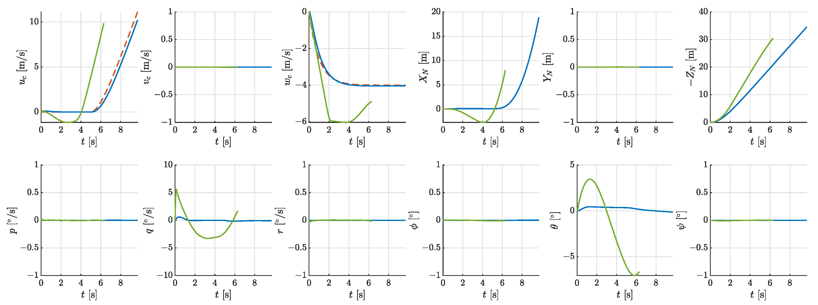
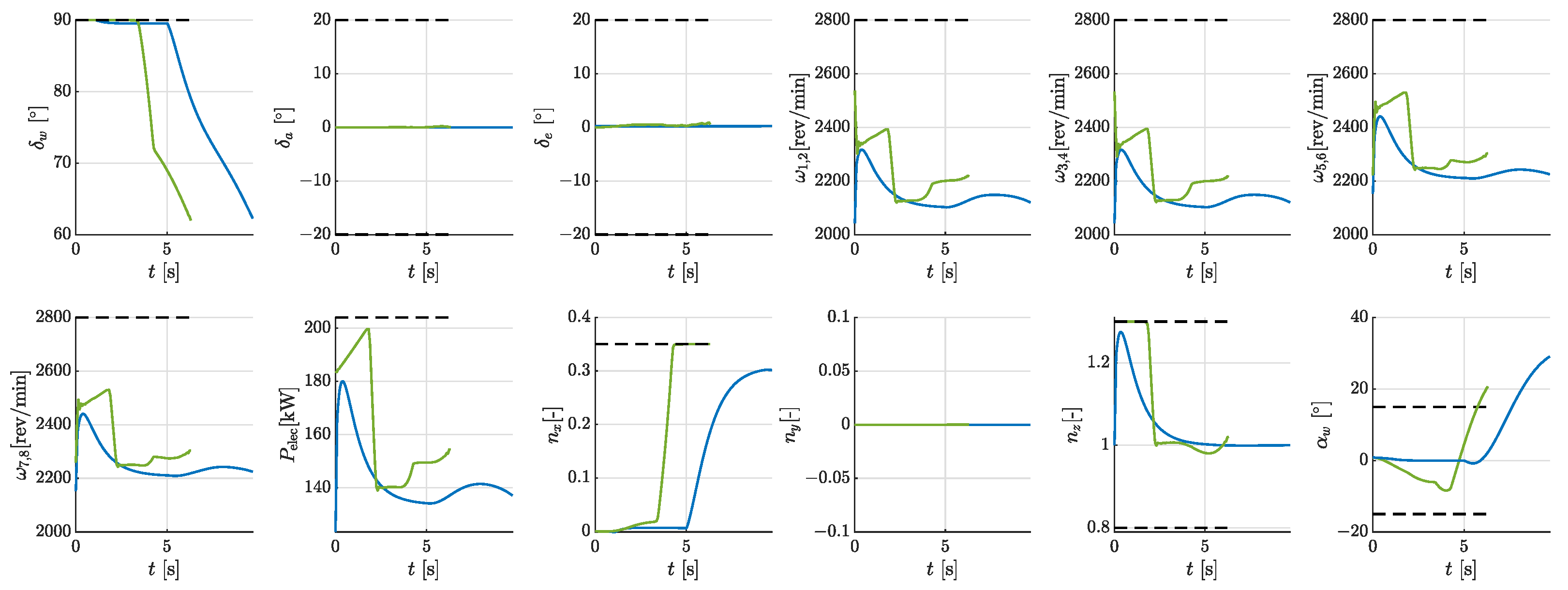
4.1. Phase 1—Initial Take-Off

In the first take-off phase, the aircraft is supposed to rise vertically off the ground, then accelerate to $V_{\mathrm{TOSS}}$ and achieve a positive rate of climb. Boundary conditions and path constraints in this phase are listed in Table 7. We first tried solving this single-phase OCP using the FALCON.m software (version 1.30) with its default initial guess, a “straight-line interpolation” between the initial and terminal boundary conditions. However, this failed to yield a solution despite the OCP comprising only one phase.

To generate a viable initial guess, we designed straightforward pilot commands $u_{\mathrm{c},\mathrm{cmd}}$ and $w_{\mathrm{c},\mathrm{cmd}}$ to execute the mission in the first phase, as recorded in Figure 5 and Figure 6. The simulated trajectory adhered to the control constraints in Table 5 because they were addressed in the control allocation. Moreover, the pilot commands were smooth enough that other constraints in Table 4 and Table 6 were also satisfied. Consequently, the simulated trajectory stood as a feasible solution to the single-phase OCP. Utilizing this trajectory as the initial guess, FALCON.m successfully solved the OCP. A relatively large optimality tolerance (1 × 10⁻³) was used to obtain a sub-optimal solution with fewer iterations. Given that this solution serves only as a part of the initial guess for the complete multi-phase problem, achieving full optimality at this stage was not deemed necessary.

4.2. Phase 2—First Climb Segment

Table 1 indicates that, following the initial take-off, the aircraft needs to climb to 61 m (200 ft) above the take-off elevation $h_2$. This phase is characterized by a climb gradient exceeding 4.5% and an airspeed greater than $V_{\mathrm{TOSS}}$ at every point along the trajectory. To generate an initial guess for this phase, we employed a procedure similar to the first phase. Initially, we used a constant command $w_{\mathrm{c},\mathrm{cmd}}=-5\mathrm{m}/\mathrm{s}$ and a ramp signal command $u_{\mathrm{c},\mathrm{cmd}}$ to execute the climbing task. This simulation began from the final state of the first take-off phase solution. By leveraging the simulated trajectory as the initial guess, we computed a sub-optimal trajectory for the second phase, as depicted in Figure 7 and Figure 8. Figure 9 illustrates both the simulated flight paths and the sub-optimal paths for the first and second phases. Noticeable differences were observed between the simulation results and the sub-optimal trajectories. These differences arose because the INDI simulations provided only feasible solutions without “optimality” regarding energy efficiency. The primary role of these simulations was to establish a viable initial guess, facilitating the subsequent optimization.

4.3. Phase 3—Second Climb Segment and Phase 4—Turning

In the third take-off phase, the eVTOL is expected to accelerate to $V_{\mathrm{FTO}}$ and reach 305 m (1000 ft) above the take-off elevation $h_2$. The eVTOL should maintain a minimum climb gradient of 2.5% during this segment. Upon reaching $V_{\mathrm{FTO}}$, the aircraft proceeds to the fourth phase, changing the heading angle while maintaining at least level flight (no descent). We set the direction change to 90${}^{\circ }$ and assumed the aircraft would reach a predefined way-point. Boundary conditions and path constraints in the third and fourth take-off phases are outlined in Table 7.

To achieve the climbing task in the third phase, we employed pilot commands similar to those used in the second phase, enabling the aircraft to reach the desired velocity and altitude. For the turning task in the fourth phase, a constant yaw rate command ${\dot{\psi }}_{\mathrm{cmd}}=5^{\circ }$/s was applied until the direction changed by 90${}^{\circ }$. While the simulated trajectory was dynamically feasible, it did not precisely fulfill all final boundary conditions. To address this discrepancy, these final boundary conditions were incorporated into the cost function as soft penalties. Subsequently, a sub-optimal trajectory was computed for this phase. The simulated and sub-optimal trajectories are recorded in Figure 10 and Figure 11.

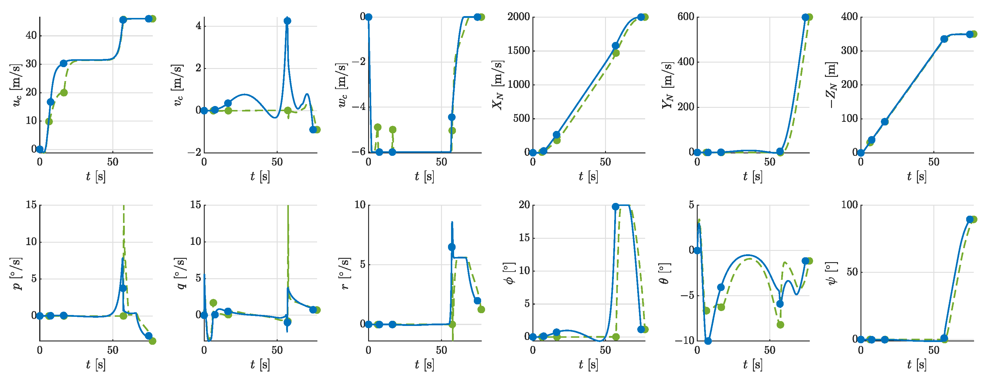
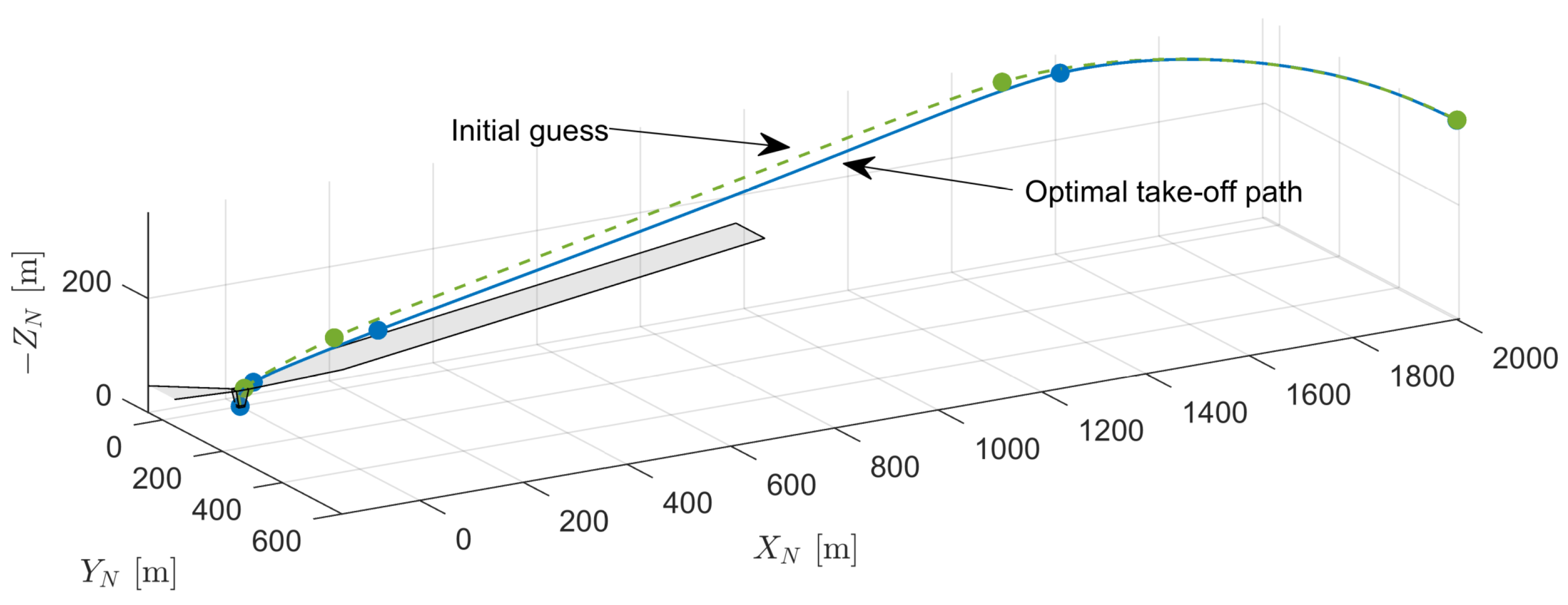
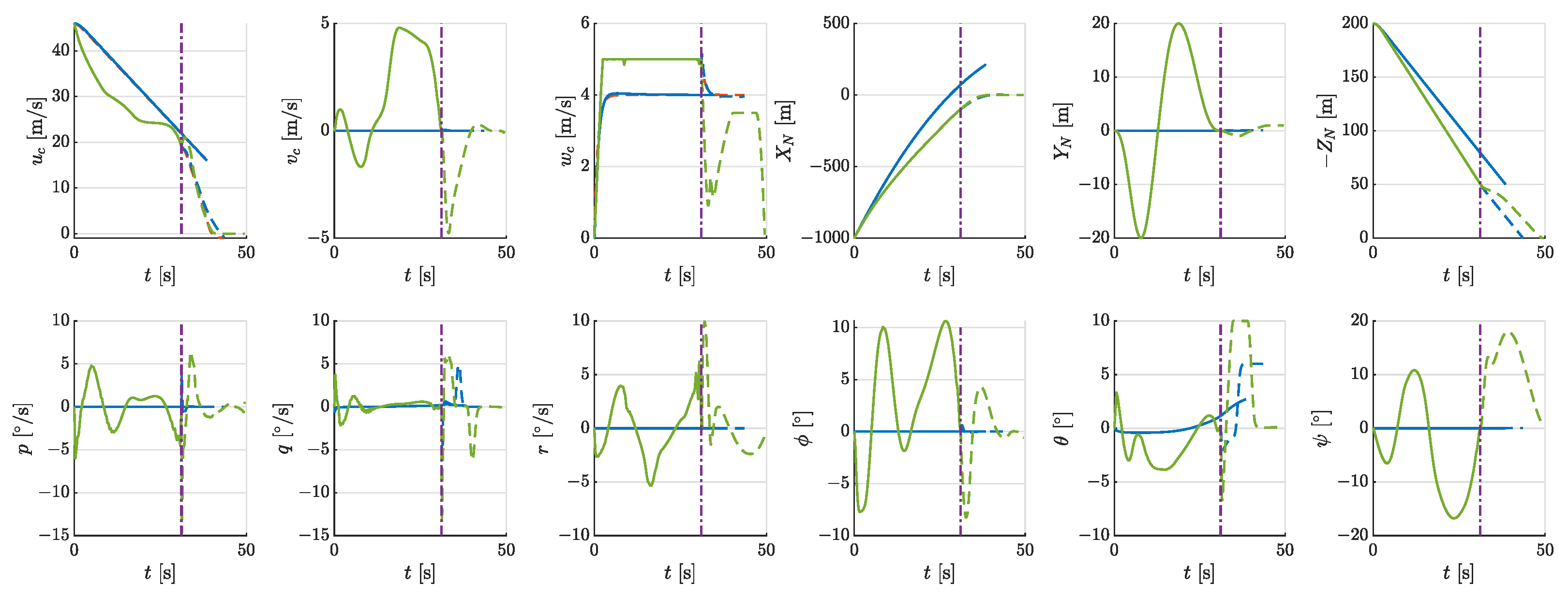
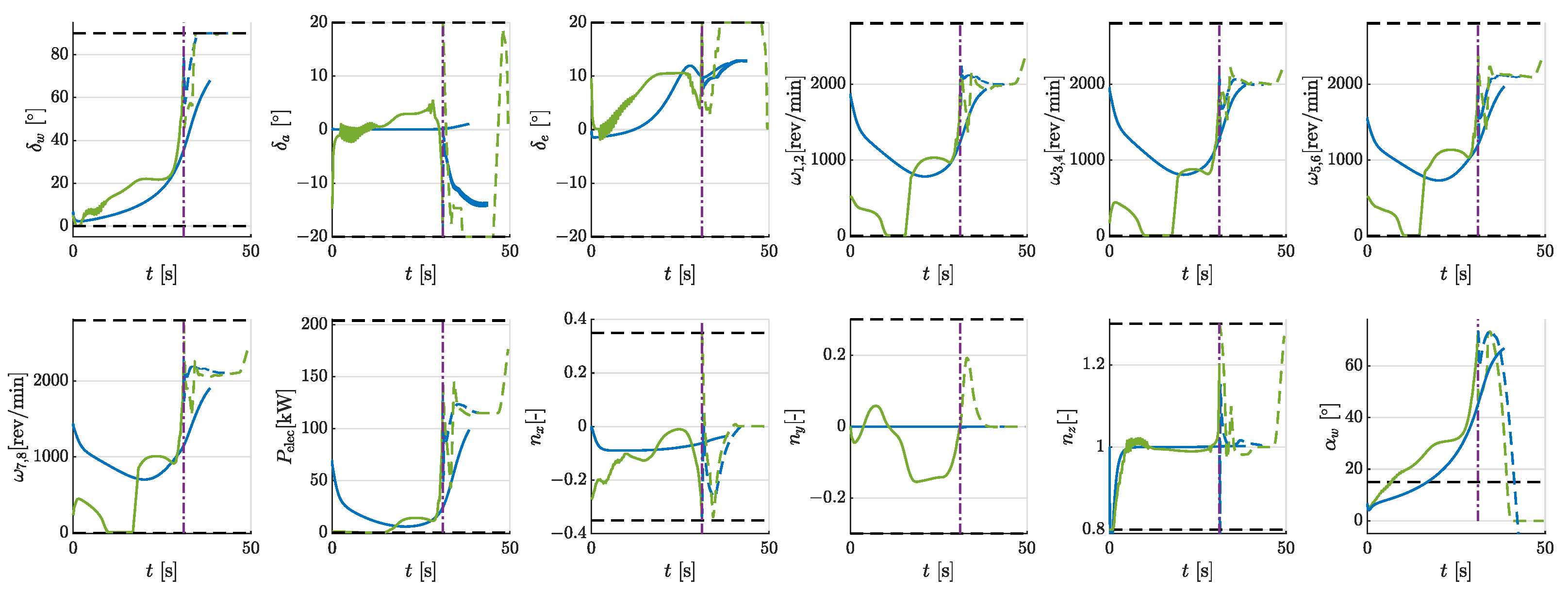
4.4. Multi-Phase Take-Off Trajectory

In the previous subsections, we employed the INDI controller to execute flight tasks within each phase. The simulated trajectory not only served as an initial guess for the OCP, but also offered a baseline for setting scaling factors and discretization size. Subsequently, a sub-optimal flight trajectory was computed for each phase. The straightforward concatenation of these single-phase trajectories yielded a feasible and sub-optimal initial guess for the original multi-phase problem. The final NLP involved 9390 optimization variables, 5928 equality constraints, and 8898 inequality constraints. Both optimality tolerance and feasibility tolerance are set to 1 × 10⁻⁵. While the solution process that started with the default “straight-line interpolation” initial guess failed to converge, FALCON.m successfully found a converged solution with the feasible initial guess after 367 iterations. The computational time for the entire process was 115.4 s, executed on a laptop equipped with an AMD Ryzen 5 3500U CPU and 8 GB of RAM.

Time histories of the optimal trajectory and the initial guess are compared in Figure 12 and Figure 13. Figure 14 illustrates the take-off paths. The feasible initial guess resulted in energy consumption of 7,146,100 joules (1.99 kWh) in 77.22 s, while the optimal take-off trajectory consumed 6,784,800 joules (1.88 kWh) within 74.59 s. These comparisons show that the initial guess is in the proximity of the optimal solution and thus facilitates a successful solution of the original problem by the numeric optimizer.

A detailed analysis of each phase is as follows:

• Phase 1 (0–7.41 s): The aircraft pitched downward and decreased the wing-tilt angle from 90${}^{\circ }$ to 52${}^{\circ }$, climbing and accelerating with almost the maximum power. The energy consumption was 0.34 kWh, and the average power was 167 kW.
• Phase 2 (7.41 s–16.31 s): The tilt angle decreased to 32${}^{\circ }$. The aircraft further accelerated to near stall speed, with the power reduced to 40% of the maximum power. The energy consumption was 0.25 kWh, and the average power was 101 kW.
• Phase 3 (16.31 s–57.02 s): The wings stop tilting forward. The aircraft maintained a climb near the stall speed. Toward the end of this phase, it accelerated to $V_{\mathrm{FTO}}$ at maximum power. The energy consumption was 0.93 kWh, and the average power was 83 kW.
• Phase 4 (57.02 s–74.59 s): The aircraft operated at its lowest power, making a 90-degree turn with a roll angle of 20 degrees and a turning rate of approximately $5.6^{\circ }/\mathrm{s}$. The energy consumption was 0.36 kWh, and the average power was 74 kW.

This analysis reveals that the aircraft required the highest average power demand in the hover flight (Phase 1), though its duration was relatively brief, contributing approximately 18% to the total energy consumption in take-off. The transition flight, encompassing Phases 2 and 3, saw a reduction in average power but accounted for over 60% of the total energy expenditure. Lastly, in the turning task (Phase 4), the power requirement was at its lowest, with energy consumption constituting 19% of the total. The strategy employed during take-off to save energy is also notable. During Phase 3, the aircraft maintained a speed of approximately 32 m/s most of the time and accelerated rapidly to $V_{\mathrm{FTO}}$ in the later stage. This behavior can be attributed to the low power demand at a forward speed of 32 m/s during ascent. Increasing the forward speed further may lead to a higher advance ratio of the propellers, reducing overall efficiency.

Notably, the last subplot in Figure 13 shows that the wings’ angle of attack surpassed the stall angle in Phase 2. Since the aircraft predominantly relies on the propulsion system during transition flight, this “stall” is acceptable and does not lead to unsafe behaviors of the aircraft. This phenomenon also highlights the necessity for a dynamics model with an aerodynamics database extending into the “post-stall” region.

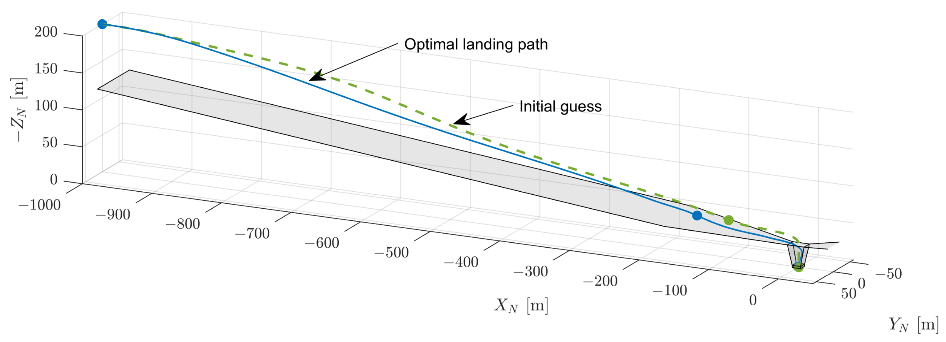
5. Vertical Landing Trajectory Optimization

The vertical landing trajectory is divided into two phases: (1) Approach to the Landing Decision Point (LDP), and (2) Land on the vertiport. The approach starts from a predefined way-point, and the LDP height is 50 m. The boundary conditions and path constraints for the two landing phases are listed in

Table 8. Phase-specific constraints in landing.

Phase	Initial Condition	Final Condition	Path Constraints
1	${[u_{\mathrm{b}},v_{\mathrm{b}},w_{\mathrm{b}}]}^T={[46\mathrm{m}/\mathrm{s},0,0]}^T$ ${[p,q,r]}^T={[0,0,0]}^T$ ${[\varphi ,\theta ,\psi ]}^T={[0,0,0]}^T$ ${[X_N,Y_N,Z_N]}^T=$ ${[1000\mathrm{m},0,-200\mathrm{m}]}^T$	$Z_N=-50\mathrm{m},V_{\mathrm{a}}\le 20\mathrm{m}/\mathrm{s}$	Obstacle limitation surface
2	Final state of the first landing phase solution	${[u_{\mathrm{b}},v_{\mathrm{b}},w_{\mathrm{b}}]}^T={[0,0,0]}^T$ ${[p,q,r]}^T={[0,0,0]}^T$ ${[\varphi ,\theta ,\psi ]}^T={[0,0,0]}^T$ ${[X_N,Y_N,Z_N]}^T={[0,0,0]}^T$	Obstacle limitation surface Obstacle-free volume $w_{\mathrm{c}}\le 4\mathrm{m}/\mathrm{s}$

. The optimal control problem is similar to the take-off process in Equation (15), except that the phase-specific constraints are from Table 8.

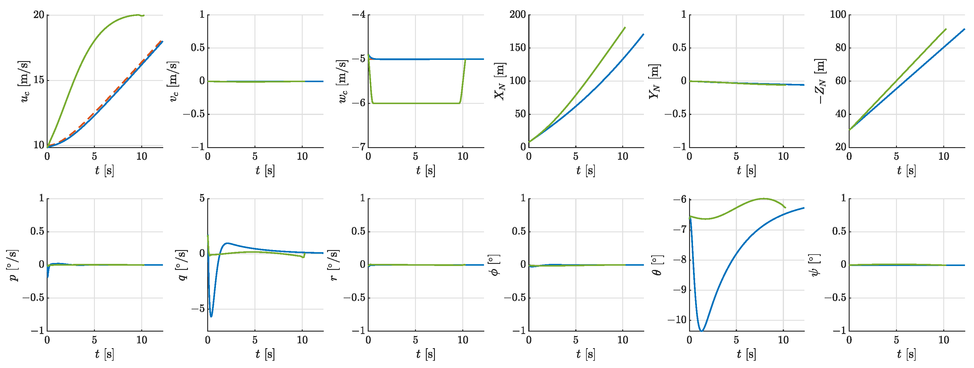
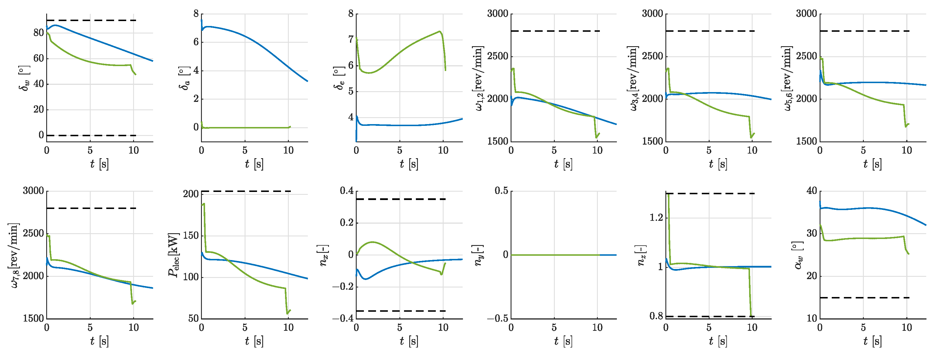
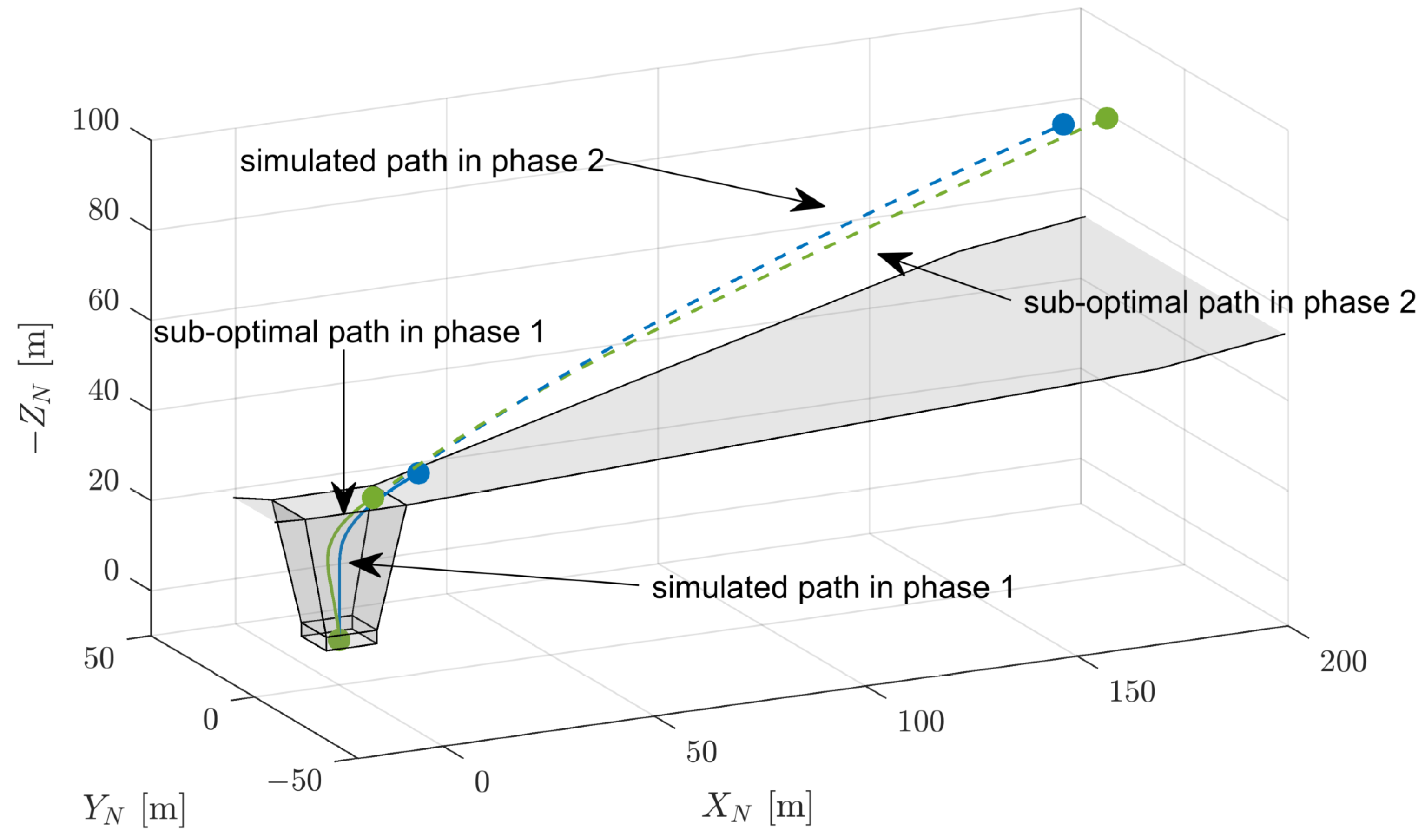
5.1. Individual Phases

As described in Section 4, we initially formulated pilot commands to execute the approach task, including decreasing forward speed $u_{\mathrm{c},\mathrm{cmd}}$ and a constant sink rate $w_{\mathrm{c},\mathrm{cmd}}$. A sub-optimal approach trajectory was subsequently generated using the simulated trajectory as the initial guess.

For the landing phase, we “manually” landed the eVTOL aircraft starting from the terminal state of the approach trajectory. Given the INDI controller in Figure 4, a precise landing was challenging since position control was not available. The objective was not to achieve a perfect landing at the vertiport but to establish a reasonable and dynamically feasible landing trajectory. Unfulfilled boundary conditions were incorporated into the OCP as soft penalties, making the simulated trajectory a plausible initial guess for generating a sub-optimal landing trajectory. Figure 15 and Figure 16 present both the simulated and sub-optimal trajectories for the approach and landing phases.

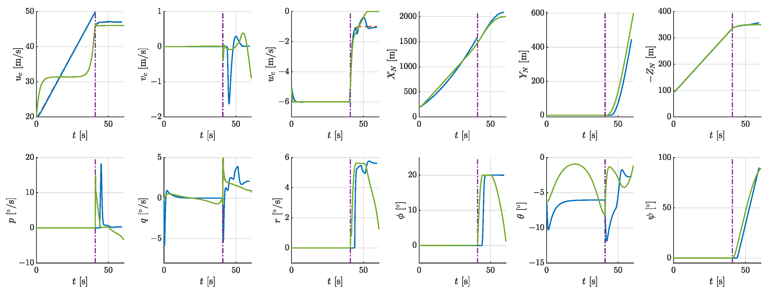
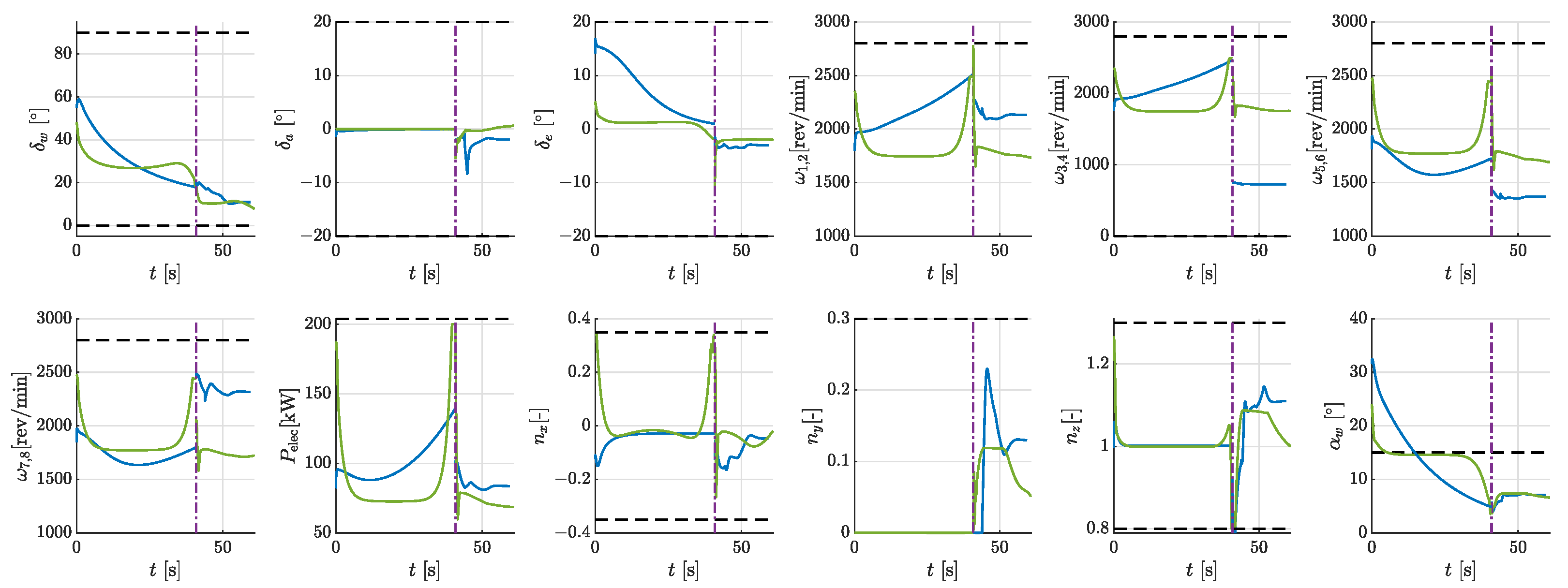
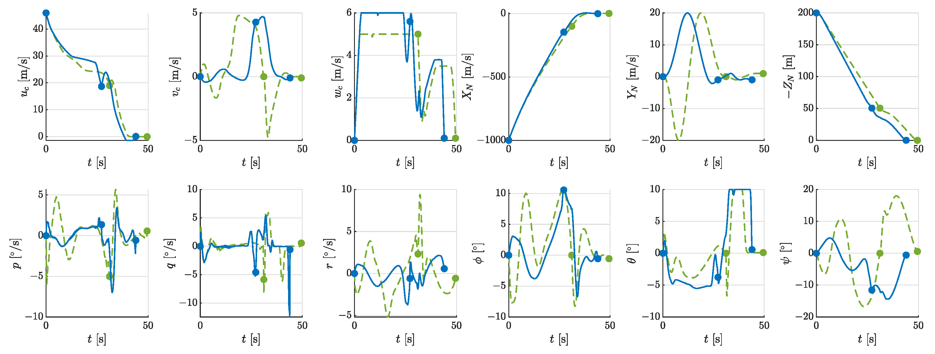
5.2. Multi-Phase Landing Trajectory

To solve the complete landing trajectory problem, 151 equidistant discretization nodes were assigned to each phase. The final NLP involved 5740 optimization variables, 3624 equality constraints, and 4985 inequality constraints. FALCON.m successfully found a converged solution using the feasible initial guess in 76 s, involving 793 iterations. Time histories of the optimal trajectory and the initial guess are presented in Figure 17 and Figure 18, and three-dimensional approach and landing paths are compared in Figure 19. The energy consumption of the initial guess was 2,351,200 joules (0.65 kWh), while the optimal solution consumed 1,768,200 joules (0.49 kWh).

A detailed analysis of each phase is as follows:

• Phase 1 (0–27.17 s): Characterized by minimal propeller rotational speeds, this phase exhibited negligible total power. The aircraft decelerated to the landing reference speed $V_{\mathrm{REF}}$ by increasing the tilt angle, resulting in almost zero energy consumption.
• Phase 2 (27.17 s–43.98 s): The tilt angle rapidly increased to 90${}^{\circ }$, and the propellers produced sufficient lift to counteract gravity. Meanwhile, the aircraft pitched upward to further decelerate its forward speed. This phase involved coordinated position, velocity, and attitude adjustment to achieve zero values at touchdown. The energy consumption was 0.48 kWh, with an average power of 104 kW.

The aircraft expended most energy in the final landing phase, while it primarily relied on aerodynamic lift and required minimal propulsive effort in the approach phase. Deceleration in the approach was mainly achieved through increasing the wings’ angle of attack. Upon reaching the LDP, the aircraft increased propeller thrust, allowing it to descend at a slower sink rate and further reduce the forward speed. The energy consumption during landing amounted to approximately 26% of the energy expended during take-off. Notably, Figure 18 reveals that the wings’ angle of attack reached substantial values during landing.

6. Conclusions

This paper has presented a procedure for optimizing eVTOL take-off and landing trajectories, accounting for various operational constraints and integrating 6DOF dynamics to ensure trajectory precision and feasibility. The key conclusions are as follows:

• The flight trajectory is segmented into multiple phases, each tailored to unique constraints, considering vertical take-off and landing complexities and airworthiness requirements.
• Integrating 6DOF dynamics in the multi-phase problem results in a large-scale NLP that necessitates a good initial guess. The INDI control simplifies vehicle operation. Simulated trajectories exhibit dynamic feasibility and provide viable initial guesses for generating sub-optimal trajectories within individual phases. Concatenating these sub-optimal trajectories forms a feasible initial guess for the original multi-phase problem.
• Successful computation of energy-minimum take-off and landing trajectories for a tilt-wing eVTOL is demonstrated. In take-off, the hover flight demands the highest power, while the transition flight consumes the most energy, over 60%. To save energy, the eVTOL aircraft maintains a favorable forward speed at about 32 m/s for a long duration, accelerating to the final take-off speed primarily toward the end of the transition. In landing, the bulk of energy consumption transpires in the final landing, with total energy in landing being about 26% of that in take-off.
• The tilt-wings’ angle of attack manifests large values during take-off and landing, suggesting that enforcing the stall angle as a strict constraint in low-speed VTOL operations may not be necessary.

The pilot commands to the INDI controller were designed “manually” in this paper. Automating the generation of pilot commands is a potential avenue for future research. Such automation could be implemented through a higher-level control function integrated within the INDI framework. Moreover, the employed INDI controller can be adapted into a trajectory tracking controller. Furthermore, the effects of meteorological conditions in the urban area such as winds and turbulences on optimal trajectories may also be investigated.

References

1. Boeing Wisk. Concept of Operations for Uncrewed Urban Air Mobility; The Boeing Company: Arlington, VA, USA, 2022; Available online: www.boeing.com/innovation/con-ops (accessed on 1 November 2023).
2. European Union Aviation Safety Agency. Special Condition for Small-Category VTOL Aircraft; European Union Aviation Safety Agency: Cologne, Germany, 2019. Available online: www.easa.europa.eu/en/downloads/99957/en (accessed on 1 November 2023).
3. European Union Aviation Safety Agency. Second Publication of Proposed Means of Compliance with the Special Condition VTOL; European Union Aviation Safety Agency: Cologne, Germany, 2022. Available online: www.easa.europa.eu/en/downloads/137443/en (accessed on 1 November 2023).
4. European Union Aviation Safety Agency. Vertiports Prototype Technical Specifications for the Design of VFR Vertiports for Operation with Manned VTOL-Capable Aircraft Certified in the Enhanced Category; European Union Aviation Safety Agency: Cologne, Germany, 2022. Available online: www.easa.europa.eu/en/downloads/136259/en (accessed on 1 November 2023).
5. Civil Aviation Administration of China. Special Conditions for EHang EH216-S Unmanned Aircraft System: SC-21-002; Civil Aviation Administration of China: Beijing, China, 2022; (In Chinese). Available online: www.caac.gov.cn/XXGK/XXGK/BZGF/ZYTJHHM/202202/t20220222_211914.html (accessed on 1 November 2023).
6. Federal Aviation Administration. Airworthiness Criteria: Special Class Airworthiness Criteria for the Joby Aero, Inc. Model JAS4-1 Powered-Lift: FAA-2021-0638; Federal Aviation Administration: Washington, DC, USA, 2022. Available online: www.federalregister.gov/documents/2022/11/08/2022-23962/airworthiness-criteria-special-class-airworthiness-criteria-forthe-joby-aero-inc-model-jas4-1 (accessed on 1 November 2023).
7. Federal Aviation Administration. Airworthiness Criteria: Special Class Airworthiness Criteria for the Archer Aviation Inc. Model M001 Powered-Lift: FAA-2022-1548; Federal Aviation Administration: Washington, DC, USA, 2022. Available online: www.federalregister.gov/documents/2022/12/20/2022-27445/airworthiness-criteria-special-class-airworthiness-criteria-forthe-archer-aviation-inc-model-m001 (accessed on 1 November 2023).
8. Federal Aviation Administration. Engineering Brief No. 105, Vertiport Design: EB No. 105; Federal Aviation Administration: Washington, DC, USA, 2022. Available online: www.faa.gov/airports/engineering/engineering_briefs/engineering_brief_105_vertiport_design (accessed on 1 November 2023).
9. Pradeep, P.; Wei, P. Energy-efficient arrival with rta constraint for multirotor evtol in urban air mobility. J. Aerosp. Inf. Syst. 2019, 16, 263–277. [Google Scholar] [CrossRef]
10. Chauhan, S.S.; Martins, J.R. Tilt-wing eVTOL takeoff trajectory optimization. J. Aircr. 2020, 57, 93–112. [Google Scholar] [CrossRef]
11. Doff-Sotta, M.; Cannon, M.; Bacic, M. Fast optimal trajectory generation for a tiltwing VTOL aircraft with application to urban air mobility. In Proceedings of the 2022 American Control Conference (ACC), Atlanta, GA, USA, 8–10 June 2022; pp. 4036–4041. [Google Scholar]
12. Lu, Z.; Li, H.; He, R.; Holzapfel, F. Energy-Efficient Incremental Control Allocation for Transition Flight via Quadratic Programming. In Proceedings of the International Conference on Guidance, Navigation and Control, Harbin, China, 5–7 August 2022; Springer: Singapore, 2022; pp. 4940–4951. [Google Scholar]
13. Piprek, P.; Holzapfel, F. Robust Trajectory Optimization of VTOL Transition Maneuver Using Bi-Level Optimal Control. In Proceedings of the 31st Congress of the International Council of the Aeronautica Science, Belo Horizonte, Brazil, 9–14 September 2018. [Google Scholar]
14. Wang, M.; Diepolder, J.; Zhang, S.; Söpper, M.; Holzapfel, F. Trajectory optimization-based maneuverability assessment of eVTOL aircraft. Aerosp. Sci. Technol. 2021, 117, 106903. [Google Scholar] [CrossRef]
15. Krammer, C.; Schweighofer, F.; Gierszewski, D.; Scherer, S.; Akman, T.; Hong, H.; Holzapfel, F. Requirements-based Generation of Optimal Vertical Takeoff and Landing Trajectories for Electric Aircraft. In Proceedings of the 33rd Congress of the International Council of the Aeronautical Sciences (ICAS), Stockholm, Sweden, 4–9 September 2022. [Google Scholar]
16. Lu, Z.; Hong, H.; Diepolder, J.; Holzapfel, F. Maneuverability Set Estimation and Trajectory Feasibility Evaluation for eVTOL Aircraft. J. Guid. Control. Dyn. 2023, 46, 1184–1196. [Google Scholar] [CrossRef]
17. Akman, T.; Schweighofer, F.; Afonso, R.; Ben-Asher, J.; Holzapfel, F. Robust eVTOL trajectory optimization under uncertainties–Challenges and approaches. Proc. J. Phys. Conf. Ser. 2023, 2514, 012002. [Google Scholar] [CrossRef]
18. Fisch, F. Development of a Framework for the Solution of High-Fidelity Trajectory Optimization Problems and Bilevel Optimal Control Problems. Ph.D. Thesis, Technische Universität München, München, Germany, 2011. [Google Scholar]
19. Bittner, M.; Fisch, F.; Holzapfel, F. A multi-model gauss pseudospectral optimization method for aircraft trajectories. In Proceedings of the AIAA Atmospheric Flight Mechanics Conference, Minneapolis, MN, USA, 13–16 August 2012; p. 4728. [Google Scholar]
20. Lu, Z.; Hong, H.; Gerdts, M.; Holzapfel, F. Flight Envelope Prediction via Optimal Control-Based Reachability Analysis. J. Guid. Control. Dyn. 2022, 45, 185–195. [Google Scholar] [CrossRef]
21. Federal Aviation Administration. Flight Test Guide for Certification of Transport Category Airplanes, AC No: 25-7D; Federal Aviation Administration: Washington, DC, USA, 2018. Available online: https://www.faa.gov/documentLibrary/media/Advisory_Circular/AC_25-7D.pdf (accessed on 1 November 2023).
22. May, M.S.; Milz, D.; Looye, G. Dynamic modeling and analysis of tilt-wing electric vertical take-off and landing vehicles. In Proceedings of the AIAA SciTech 2022 Forum, San Diego, CA, USA, 3–7 January 2022; p. 0263. [Google Scholar]
23. Holzapfel, F. Nichtlineare Adaptive Regelung eines Unbemannten Fluggerätes. Ph.D. Thesis, Technische Universität München, München, Germany, 2004. [Google Scholar]
24. Sieberling, S.; Chu, Q.; Mulder, J. Robust flight control using incremental nonlinear dynamic inversion and angular acceleration prediction. J. Guid. Control. Dyn. 2010, 33, 1732–1742. [Google Scholar] [CrossRef]
25. Harris, J.J. F-35 flight control law design, development and verification. In Proceedings of the 2018 Aviation Technology, Integration, and Operations Conference, Atlanta, GA, USA, 25–29 June 2018; p. 3516. [Google Scholar]
26. Lu, Z.; Tang, P.; Zhang, S. Incremental nonlinear dynamic inversion based control allocation approach for a BWB UAV. In Proceedings of the 2018 IEEE CSAA Guidance, Navigation and Control Conference (CGNCC), Xiamen, China, 10–12 August 2018; pp. 1–6. [Google Scholar]
27. Li, H.; Myschik, S.; Holzapfel, F. Null-Space-Excitation-Based Adaptive Control for an Overactuated Hexacopter Model. J. Guid. Control. Dyn. 2023, 46, 483–498. [Google Scholar] [CrossRef]
28. Raab, S.A.; Zhang, J.; Bhardwaj, P.; Holzapfel, F. Proposal of a unified control strategy for vertical take-off and landing transition aircraft configurations. In Proceedings of the 2018 Applied Aerodynamics Conference, Atlanta, GA, USA, 25–29 June 2018; p. 3478. [Google Scholar]
29. Lombaerts, T.; Kaneshige, J.; Schuet, S.; Hardy, G.; Aponso, B.L.; Shish, K.H. Nonlinear dynamic inversion based attitude control for a hovering quad tiltrotor eVTOL vehicle. In Proceedings of the AIAA Scitech 2019 Forum, San Diego, CA, USA, 7–11 January 2019; p. 0134. [Google Scholar]
30. Zhang, J.; Bhardwaj, P.; Raab, S.A.; Saboo, S.; Holzapfel, F. Control allocation framework for a tilt-rotor vertical take-off and landing transition aircraft configuration. In Proceedings of the 2018 Applied Aerodynamics Conference, Atlanta, GA, USA, 25–29 June 2018; p. 3480. [Google Scholar]
31. Rieck, M.; Bittner, M.; Grüter, B.; Diepolder, J.; Piprek, P.; Göttlicher, C.; Schwaiger, F.; Hosseini, B.; Schweighofer, F.; Akman, T.; et al. FALCON.m User Guide; Institute of Flight System Dynamics, Technical University of Munich: München, Germany, 2023. [Google Scholar]
32. Wächter, A.; Biegler, L.T. On the implementation of an interior-point filter line-search algorithm for large-scale nonlinear programming. Math. Program. 2006, 106, 25–57. [Google Scholar] [CrossRef]
Figure 1. Vertical take-off and landing paths, adapted from [3]. Solid lines: take-off path, dashed lines: landing path, O: aircraft parking site, A: take-off decision point (TDP), B: the point where the take-off safety speed V TOSS is reached, C: 61 m higher than h 2 , D: the point where the final take-off speed V FTO is reached, E: start of approach, and F: landing decision point (LDP).
Aerospace 11 00039 g001
Figure 2. The VTOL procedure volume and the obstacle-free volume, adapted from [3,4].
Aerospace 11 00039 g002
Figure 3. Configuration of the tilt-wing eVTOL aircraft, adapted from [22].
Aerospace 11 00039 g003
Figure 4. INDI control structure with highlighted modules.
Aerospace 11 00039 g004
Figure 5. Flight states in the first take-off phase. Red: pilot commands, blue: simulation, green: sub-optimal trajectory.
Aerospace 11 00039 g005
Figure 6. Control inputs and output variables in the first take-off phase. Blue: simulation, green: sub-optimal trajectory, black: constraints.
Aerospace 11 00039 g006
Figure 7. Flight states in the second take-off phase. Red: pilot commands, blue: simulation, green: sub-optimal trajectory.
Aerospace 11 00039 g007
Figure 8. Control inputs and output variables in the second take-off phase. Blue: simulation, green: sub-optimal trajectory, black: constraints.
Aerospace 11 00039 g008
Figure 9. Flight paths in the first and second take-off phases. Blue: simulation, green: sub-optimal trajectory, grey: obstacle-free volume and obstacle limitation surfaces.
Aerospace 11 00039 g009
Figure 10. Flight states in the third and fourth take-off phases. Red: pilot commands, blue: simulation, green: sub-optimal trajectory.
Aerospace 11 00039 g010
Figure 11. Control inputs and output variables in the third and fourth take-off phases. Blue: simulation, green: sub-optimal trajectory, black: constraints.
Aerospace 11 00039 g011
Figure 12. Time histories of states in take-off. Blue: optimal solution, green: initial guess.
Aerospace 11 00039 g012
Figure 13. Time histories of controls and outputs in take-off. Blue: optimal solution, green: initial guess, black: constraints.
Aerospace 11 00039 g013
Figure 14. The optimal multi-phase take-off path and its initial guess. Blue: optimal solution, green: initial guess, grey: obstacle-free volume and obstacle limitation surfaces.
Aerospace 11 00039 g014
Figure 15. Flight states in the two landing phases. Red: pilot commands, blue: simulation, green: sub-optimal trajectory.
Aerospace 11 00039 g015
Figure 16. Control inputs and output variables in the two landing phases. Blue: simulation, green: sub-optimal trajectory, black: constraints.
Aerospace 11 00039 g016
Figure 17. Time histories of states in landing. Blue: optimal solution, green: initial guess.
Aerospace 11 00039 g017
Figure 18. Time histories of controls and outputs in landing. Blue: optimal solution, green: initial guess, black: constraints.
Aerospace 11 00039 g018
Figure 19. The optimal multi-phase landing path and the initial guess. Blue: optimal solution, green: initial guess, grey: obstacle-free volume and obstacle limitation surfaces.
Aerospace 11 00039 g019