Article

Model-Reference Reinforcement Learning for Safe Aerial Recovery of Unmanned Aerial Vehicles

1
School of Astronautics, Harbin Institute of Technology, Harbin 150001, China
2
Avic Aerodynamics Research Institute, Shenyang 110034, China
*
Author to whom correspondence should be addressed.
Aerospace 2024, 11(1), 27; https://doi.org/10.3390/aerospace11010027
Submission received: 10 November 2023 / Revised: 24 December 2023 / Accepted: 26 December 2023 / Published: 27 December 2023

Abstract

:
In this study, we propose an aerial rendezvous method to facilitate the recovery of unmanned aerial vehicles (UAVs) using carrier aircrafts, which is an important capability for the future use of UAVs. The main contribution of this study is the development of a promising method for online generation of feasible rendezvous trajectories for UAVs. First, the wake vortex of a carrier aircraft is analyzed using the finite element method, and a method for establishing a safety constraint model is proposed. Subsequently, a model-reference reinforcementearning algorithm is proposed based on the potential function method, which can ensure the convergence and stability of training. A combined reward function is designed to solve the UAV trajectory generation problem under non-convex constraints. The simulation results show that, compared with the traditional artificial potential field method under different working conditions, the success rate of this method under non-convex constraints is close to 100%, with high accuracy, convergence, and stability, and has greater application potential in the aerial recovery scenario, providing a solution to the trajectory generation problem of UAVs under non-convex constraints.

1. Introduction

Aerial recovery is a new technology that can quickly and efficiently capture unmanned aerial vehicle (UAV) in the air when there are no suitable platforms foranding onand or sea [1,2]. Swarm UAVs areow-cost and reusable devices that can be quickly deployed and have recently attracted considerable research interest [3]. A carrier aircraft transports a swarm of UAVs to the edge of a combat zone and releases them. Swarm UAVs then return to the carrier aircraft after completing their tasks. Aerial recovery can improve combat performance, reuse rate, and flexibility of UAVs. However, this involves docking the probe of the UAVs with a cable-drogue assembly towed by the carrier aircraft and then pulling it into the cabin with a winch. The idea of “aerial recovery” has gained interest since theaunch of the Defense Advanced Research Projects Agency (DARPA)’s “Gremlins” project (2016) [4]. On 29 October 2021, DARPA successfully recovered an X-61 “Gremlin” drone in mid-air for the first time [5,6]. Studies have shown that wake vortices have a significant impact on the flight safety of aircrafts [7]. If a following aircraft breaks into the wake area of aeading aircraft, the aerodynamic force of the following aircraft is significantly disturbed [8].
In this case, the main challenges of UAV aerial recovery can be summarized as follows: (1) describing the unsafe area for rendezvous and docking missions while accounting for the effects of wake vortices and turbulence from the carrier aircraft; (2) obtaining closer proximity to the carrier while avoiding unsafe areas, which will reduce theength of the recovery rope, thereby reducing the difficulty of dragging the drone back into the cabin and increasing efficiency; (3) the development of an online real-time control algorithm that ensures safety and accessibility.
Current research methods for wake vortices can be roughly divided into experimental measurement methods, theoretical analyses, and numerical simulation methods based on computational fluid dynamics. The experimental methods of wake simulation include artificial simulation of experimental environment devices represented by on-site observation methods, such as wind tunnels [9]. However, these methods are time consuming, expensive, andack flexibility. In addition, some characteristics of the wake vortex flow field cannot be accurately resolved and captured through experiments owing to theimitations of the data collection and measurement methods. The theoretical analysis methods are primarily used for rapid modeling and simulation of wake vortices [10]. They cannot satisfy the computational requirements of complex shapes and high precision. Numerical simulations are based on the theory of computational fluid dynamics. With the rapid development of high-performance computer technology, these methods have been widely used in aircraft flow fields, such asarge eddy simulations (LES) and simulations based on the Reynolds-averaged Navier–Stokes (RANS) theory [11,12]. Numerical simulation methods are widely recognized for their ability to simulate wake flows in a cost-effective, convenient, and scalable manner.
Some studies have been conducted on the aerial recovery of UAVs [4,13]. Different theoretical approaches have been explored to solve the guidance and control problem [14]. These can be divided into three categories: optimization, hybrid, and analytical methods [15,16]. Examples include direct collocation [17], indirect (variational) methods [18], rapidly exploring random trees (RRTs) [19], sequential convex optimization [20], waypoint following using a PD or H-infinity controller [21], artificial potential functions (APFs) [22], second-order cone programming [23], model predictive control (MPC) [24], and adaptive control techniques [25]. However, many of these methods are offline, time-consuming, and unsuitable for non-convex optimization problems, whereas deep reinforcementearning (RL), which enables autonomous real-time, collision-free rendezvous, and proximity operations, has the potential to overcome these disadvantages [26]. One method of using deep RL is to obtain solutions for systems with complex dynamics and constraints [27]. It has the key benefit of performing well for problems that do not have a suitable nonlinear programming formulation, can generate real-time and dynamic solutions for online applications [28], and has been used in applications in real-world UAV trajectory generation and control, achieving the highest performance far beyond that of humans [29]. This can also be beneficial when the underlying problem is stochastic [30]. However, solving the potential reward sparseness when RL is used to solve UAV navigation problems is difficult [31]. In the early exploration stage of training, UAVs without expert experience do not always receive rewards after each action, rendering it difficult for the algorithm to converge [32]. Existing methods primarily include exploiting intrinsic curiosity [33,34] or information gain [35]; however, these methods mayead to performance degradation. Another method is to imitate expert experience [36]; however, the upperimit of the algorithm performance may be affected by experts, and expert data may be difficult to obtain.
In this study, we considered the aerial recovery of UAV as a reach-avoidance problem to establish a safety constraint model by analyzing the flow field around the carrier aircraft. We present an online trajectory generation method for UAVs in a three-dimensional (3D) space. The contributions of this study can be summarized as follows:
(1) The equipotential airflowines of the flow field around a carrier aircraft were depicted by finite element analysis, and a method for establishing safe constraints was proposed.
(2) A new potential function-based reinforcementearning control method (PRL) was proposed, utilizing the advantages of a model-reference RL algorithm. It can be used for trajectory generation under non-convex constraints, satisfying the safety constraints while guaranteeing convergence. This may be more efficient than RL algorithmsearned from scratch.
(3) A reward function based on a potential function was designed to ensure security while reducing the impact of sparse rewards. Simultaneously, as the training of reinforcementearning is completed in an offline environment, the call model can meet the requirements of online and real-time response in the actual application process. In addition, the convergence and stability of PRL algorithm are proved and the feasibility of the algorithm is verified through simulation experiments.

2. Problem Formulation

When performing an air-recovery mission, it is assumed that the carrier aircraft is flying at the intended cruise speed. The UAV moves to the recovery drogue, which is connected to the carrier through a cable and remains relatively stationary with the carrier. During this process, the UAV must avoid the flow field in an unsafe area around the carrier aircraft. When rendezvous occurs and the relative speed is similar, recovery drives dock with the UAV and finally return to the cabin. In this study, both UAV and drogue are regarded as mass points. A schematic diagram is shown in Figure 1.

2.1. Dynamic Model for The UAV

In this study, we considered a simplified dynamic model for a UAV [37], which can be written as
x ˙ y ˙ z ˙ v ˙ γ ˙ ψ ˙ = v cos ( ψ ) cos ( γ ) v sin ( ψ ) cos ( γ ) v sin ( γ ) u 1 u 2 u 3
where ( x , y , z ) is the position of UAV in space, v is the ground speed, ψ is the yaw angle, γ is the flight path angle, and u t = [ u 1 , u 2 , u 3 ] is the control of UAV.
As the drogue is considered to be relatively stationary with the carrier, we use p D t = [ x D , y D , z D ] to express the state vector of its position p C t = [ x C , y C , z C ] to express the position of the carrier and use p U t = [ x U , y U , z U ] to express the position of the UAV. v U t = [ x ˙ U , y ˙ U , z ˙ U ] , v D t = [ x ˙ D , y ˙ D , z ˙ D ] is the velocity of UAV and the velocity of the drogue at time step t , respectively. The speed deviation can be expressed as e v = v D t v U t = [ e v x , e v y , e v z ] , the flight path angle error between the drogue and the UAV is defined as e γ = γ U γ D , and the yaw angle error between them is defined as e ψ = ψ U ψ D . The position of the UAV relative to that of the drogue is defined as d D t = p D t p U t = [ e x , e y , e z ] .

2.2. Hazard Area Concept

The wake vortex created by the movement through the carrier can cause a variety of responses, as the air circulation can causearge rolling torques on the aircraft, which can be dangerous. Air swirling in the wake vortex has a tangential velocity that depends on its relative distance from the vortex center. A vortex has a core in which the tangential velocity increasesinearly with the radius. Outside the vortex core, the tangential velocity begins to decrease due to an inverse relationship with the radius. In order to simplify this problem, an area can be defined around the wake vortex, which is called the Hazard area. Outside this area, tangential velocityess than V 0 pose no danger to aircraft. It should be noted that the tolerance of tangential velocity is different for an aircraft with different aerodynamic parameters. The tangential velocity can be expressed as
V ω = ω y ω , y ω α V ω = Γ 2 π y ω , y ω > α
where α is the core radius, ω is the angular velocity, y ω is theocation of the wing relative to the vortexocation, and Γ is the initial vortex strength. It is related to the weight, speed, and altitude of the aircraft generating the vortex and can be expressed as
Γ 0 = 4 M C ρ v C b C π M c
where M C , v C , b C denote the mass, speed, and wingspan of the carrier aircraft inevel flight, respectively. This means that the initial strength of the vortex can be treated as a constant. Theocal variation in the aircraft’s angle of attack caused by the eddy’s current velocity field causes a rolling moment around the centerline of the wing and affects the flight of the aircraft [7], particularly for the outer region of the wake vortex, which is relevant for sizing the hazard zone because the core region must be avoided in any case [38].
The NASA Ames Research Center utilizes a numerical integration technique known as the strip theory, which uses the Biot–Savartaw to determine the induced velocity normal to the surface [39]. It determines the final rolling moment coefficient induced by the eddy currents to find aircraft danger, indicating that the numerical simulation method is feasible for establishing an unsafe area of the aircraft wake vortex. The rolling moment coefficient can be expressed as
C ω = 2 T S C b U 0 b U 2 y ω C l α V ω V T c d y ω
where T is the dynamic pressure, S C is the wing area of the carrier aircraft, b U is the span of the wake-penetrating aircraft, C l α is the wingift curve slope, V is the freestream velocity, and c is the cordength.
The simplified danger zone can help overcome the wake vortex problem. As the distance between the aircraft and the wake vortex increases, the impact on the aircraft decreases. The spatial characteristics of this phenomenon indicated the formation of a dangerous space around the wake vortex. Avoiding these areas enables safe and undisturbed flight operations [40]; thus, it can be assumed that outside the hazardous area, vortices pose no danger to the aircraft [38]. The dangerous area is based on the vortex-induced roll coefficient, which is caused by the tangential velocity. Comparing the vortex-induced roll factor to the maximum coefficient of roll supplied by the airplane control system can determine the safety of a UAV flight [7]. In this study, the non-safe area was determined using numerical analysis. When the tangential velocity of the wake vortex wasess than V ω = V 0 , the vortex-induced roll coefficient was smaller than the roll coefficient provided by the aircraft control system, as described in detail in Section 3.

3. Establishment of Safety Constraint Model

3.1. Finite Element Analysis

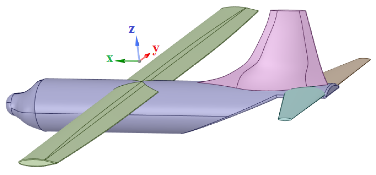
We consider a carrier aircraft with a wingspan of 40 m as an example to perform finite element analysis using ANSYS FLUENT 2021 R2. The transport aircraft model used in the experiment is shown in Figure 2. An area of block-oriented inversion encryption (BOI) was set near the aircraft to refine the grid.
A watertight geometric process was applied to divide the mesh. The minimum size of the surface grid, the maximum size, the grid of the encrypted area, and the growth rate were set to 20 mm, 10,000 mm, 500 mm, and 1.1, respectively. To capture the surface accurately, we used curvature and proximity methods to identify the curvature and microstructure. f a r is set as the pressure far-field boundary condition, s y m is set as the symmetrical surface boundary condition, and the other boundaries are set as w a l l boundaries. Finally, the volume grid is divided, and a polyhedral grid with a maximum grid size of 10,000 mm is selected. Simultaneously, a boundary–layer grid is applied to the aircraft’s surface. The final grid division results are shown in Figure 3.
In this study, the density-based steady-state solver was selected as the solution, the turbulence model was selected as the reliable k-e model, the energy equation was activated, the air density was set as an ideal gas, the viscosity was set as Sutherland, and the boundary condition was the pressure far field. This work analyzes the trailing vortex condition of the carrier aircraft at cruising altitude and cruising speed, and carries out aerial recovery of the fixed wing UAV under these conditions. The flight surface speed is 580 km/h and the flight altitude is 6 km. After the calculation, the Mach number was 0.51, the temperature was 249.18 K, and the far-field pressure was 47,217.5 Pa. The numerical solution method used in this study is a coupled algorithm in which the discrete format is second-order upwind. Theift and drag were monitored during the calculation until convergence. The flow field around a carrier aircraft is shown in Figure 4. Figure 5a shows the velocity contours and Figure 5b shows the pressure contours on the symmetry plane. Figure 6 shows the wake vortex cloud diagrams of different flow field sections, and the vector diagram of wake vortex tangential velocity in different flow field sections is shown in Figure 7.

3.2. Establishment of the Safety Constraint Model

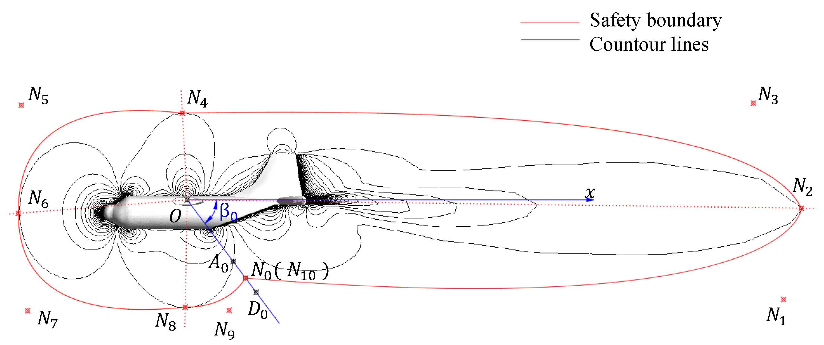
Because the ideal docking state of aerial recovery is performed on the symmetry plane ( x o z plane) of the carrier aircraft, we used a multi-segment second-order Bezier curve with n segments to establish safety constraints in this plane. Figure 6 and Figure 7 illustrate that the wake vorticity and the corresponding tangential velocity vector of the vortex center decrease as the wake vortex gradually moves away from the carrier aircraft. In addition, owing to the influence of the separation flow created by theow-pressure areas around the carrier, there are changes in the flow velocity (as shown in Figure 5), where the tangential velocity vector isess than V ω = V 0 , and the corresponding points in the flow field are projected onto the symmetry plane to obtain the contourines at the points farthest from the aircraft in all directions. We establised a polar coordinate system with the center of the wing as the origin and the speed direction of the carrier machine in the x direction, and set n to 5 to create safety constraints, as shown in Figure 8, where points N a ( l a , β a ) are the control points of the second-order Bezier curve and a is an integer from 0 to 2 n . Notably, the polar coordinate system is only established in the symmetry plane to facilitate the expression of safety constraints, and the conversion with the Cartesian coordinate system will not be expanded in detail.
We define a positive integer h that satisfies h n , and points M j ( l j , β j ) on the boundary of the constraints can be expressed as
l j = i = 0 2 l 2 h i 2 i b 2 i ( 1 b ) i β j = i = 0 2 β 2 h i 2 i b 2 i ( 1 b ) i
where b [ 0 , 1 ) , β 2 h 2 < β j < β 2 h .
The coordinates of the recovery target point (the point where the recovery drogue isocated) are determined as D 0 ( l D 0 , β 0 ) , the coordinates of the point on the equipotentialine in this direction are determined as A 0 ( l A 0 , β 0 ) , and the parameters in Figure 8 are set to satisfy the following conditions:
β 0 = arctan 2 m D g C ρ S D v d 2 π 2 l 0 l A 0 = k 1 l D 0 l 0 = k 2
where m D is the mass of the recovery drogue, g is gravity, C is the air resistance coefficient, ρ is the air density, S D is the windward area of the drogue, v d is the relative velocity of the drogue and air, and k 1 and k 2 are the expansion coefficients, usually greater than 1.

4. PRL Algorithms

In the UAV navigation problem, there are situations in which rewards are sparse, and only when the UAV completes the target task can it obtain a nonzero reward [32]. The distance between the two aircrafts always increases further in the early stages of training, owing to the high speed of the carrier aircraft. Hence, it is difficult for the UAV to obtain rewards, eading to a poor convergence of the algorithm. This difficulty is particularly evident in this problem, where at the early stage of exploration, owing to aack of expert experience and understanding of the environment, the agent will randomly choose actions, and it will take aong time to reach the goal or fail to converge at all. To solve the above problems, we propose a potential function reinforcementearning method thatearns the potential function by interacting with the environment, ensuring convergence without expert experience while avoiding the problems of being unable to reach and falling into theocal optimum.
First, the corresponding potential field function is constructed based on the hazard area established previously and the position of the carrier aircraft. By designing the corresponding reward function, the output value of the action network in the reinforcementearning algorithm is used to adjust the size of the potential function to make the UAV move toward the target position, and the purpose of avoiding the hazard area is achieved at the same time. The specific details of the algorithm will be introduced in detail in this section.

4.1. Construction of Potential Function

The APF method uses potential field gradients comprising attractive and repulsive potentials to derive the necessary control inputs to achieve the desired or target positions [22,41]. Considering this idea combined with the safety boundary model established in Section 3.2, we determine a potential field function for aerial recovery. The attractive potential τ a can be expressed as
τ a = 1 2 d D t W a d D t
where W a R 3 × 3 is a symmetric positive-definite attractive potential shaping matrix.
The repulsive potential τ b can be expressed as
τ b = d D t W b d D t 2 exp [ d S t W c d S t 1 ]
where W b , W c R 3 × 3 is a positive-definite attractive potential shaping matrix and d S t = p U t p S t is the position of the UAV relative to the target safety boundary constraint inertial position, p S t .
From a geometric perspective, shaping matrix W can be regarded as theength, width, and height of a potential function. The total potential function τ sum is defined as the sum of the attractive and repulsive potential functions as follows:
τ sum = τ a + τ b

4.2. Markov Decision Process

Generally, the RL problem is formalized using a discrete-time Markov decision process (MDP): = ( S , A , P , R , δ ) . s t S R dim ( s ) is the state vector at time t and S denotes the state space. Then, the agent takes an action a t A R dim ( a ) according to a stochastic policy/controller π a t s t . The state transition probability P defines the transition probability. In the problem studied herein, the state of the next step can be updated by inputting the state and action of the current step into the model. We assumed that the input and state data can be sampled from the system (1) at discrete time steps due to the fact that RL trains the policy network from data samples. Based on MDP, an actor–critic algorithm was proposed as theearning control framework. The detailed derivations are discussed below.

4.3. State and Action Settings

Let s t = [ e x , e y , e z , e v x , e v y , e v z ] R 6 be the state of the system at step t and the actions of RL as the coefficients of the potential function established in (9). The action of system at step t is defined as a t = [ a t a , a t b ] . Because a higher precision control is desired at the end positions, a continuous feedback control rate is chosen and defined as
u t = K a ( u t ˙ + a t a τ a + a t b τ b )
where K a R 3 × 3 is the positive gain matrix and τ a can be expressed as
τ a = d D t W a
τ b can be expressed as
τ b = exp [ 1 d S t W c d S t ] ( W b d D t ( d D t W b d D t ) W c d S t )

4.4. Setup of the RL

For standard RL, the objective is to maximize an expected accumulated return described by a value function V π ( s t ) with
V π ( s t ) = t a t π ( a t | s t ) s t + 1 P s t + 1 s t , a t ( R t + δ V π ( s t + 1 ) )
where P s t + 1 s t , a t is theikelihood of the next state s t + 1 , R t = R ( s t , a t ) is the reward function, δ [ 0 , 1 ) is a constant discount factor, and π ( a t | s t ) is called control policy in RL. Policy π ( a t | s t ) is the probability of choosing an action a t A at a state s t S . In this paper, a Gaussian policy is used, which is
π ( a | s ) = N ( a ( s ) , σ )
where N ( · , · ) stands for a Gaussian distribution with a ( s ) as the mean and σ as the covariance matrix which controls the exploration during theearning process. The Q-function used to evaluate the action can be expressed as
Q π ( s t , a t ) = R t + δ E s t + 1 [ V π ( s t + 1 ) ]
where E s t + 1 [ · ] = s t + 1 P t + 1 | t [ · ] is an expectation operator.
By introducing the entropy of policy H ( π ( a t + 1 | s t + 1 ) ) = a t π ( a t | s t ) ln ( π ( a t | s t ) ) and the temperature parameter η [42], the modified Q-function can be expressed as
Q π ( s t , a t ) = R t + δ E s t + 1 [ V π ( s t + 1 ) + η H ( π ( a t + 1 | s t + 1 ) ) ]
There are two steps that needed to be executed repeatedly in theearning process: policy evaluation and policy improvement. In the policy evaluation, the Q-value in Equation (16) is computed by applying a Bellman operation Q π ( s t , a t ) = T π Q π ( s t , a t ) where
T π Q π ( s t , a t ) = R t + δ E s t + 1 { E π [ Q π ( s t + 1 , a t + 1 ) η ln ( π ( a t + 1 | s t + 1 ) ) ] }
and the policy is improved by
π new = arg min π Π D K L ( π ( · | s t ) Z π old e 1 η Q π old ( s t , · ) )
where Π is a policy set and π old is theast updated policy. Q π old is the Q-value of π old , D K L is the Kullback–Leiber (KL) divergence [43], and Z π old is the normalization factor. Through mathematical deduction [42], Equation (18) can be written as
π * = arg min π Π E π [ η ln π ( a t | s t ) Q ( s t , a t ) ]

4.5. Rewards

In the actual process, the velocity direction of the carrier aircraft can be selected arbitrarily in the x o y plane. In this subsection, we assume that the carrier moves along the x-direction to facilitate the description of the content of the reward function.
The essence of the reward function in reinforcementearning is to communicate the goal to the agent and motivate the agent to select a strategy to achieve the goal. The goal of the agent in the action is to maximize the reward value. For UAV trajectory generation, reinforcementearning algorithms are trained using discrete reward functions. Because the agent is initially trained withittle or no knowledge of the environment, it chooses actions at random and may reach the goal over aong period [44]. However, excessively dense reward values may violate safety constraints or reduce accuracy. To address these problems, we designed a reward function for safe-RL. The reward R t is defined as
R t = C R [ R dis , R sync , R done , R safe ]
where
R dis = d d t d t R sync = d v U t v D t d t , e t e threshold 0 , e t > e threshold
are performance indicators related to distance and speed, respectively, C R = [ C dis , C sync , C done , C safe ] is the designed parameter, which is the coefficient of the rewards. e t = d t is the distance between UAV and the drogue at step t , and e threshold is the threshold that can be adjusted, after which the two agents start to synchronize their speed. R done can be expressed as follows:
R done = R d , d t < e d 0 , d t e d
where R d is aarge positive number, but its value cannot be too high; otherwise, it may cause the algorithm to fall into theocal optimum. e d is the error range that the recovery mechanism can cover, which means that entering this range can be considered a successful recovery. Distance l U , which is the distance of the carrier aircraft relative to the safe boundary constraints in the symmetry plane, can be derived from Equation (5), which is expressed as
l U = e x , e z i = 0 2 l 2 h i 2 i b U 2 i ( 1 b U ) i
where b U satisfies
β U = arctan e z e x , β 2 h 2 < β U < β 2 h i = 0 2 β 2 h i 2 i b U 2 i ( 1 b U ) i = β U , b U [ 0 , 1 )
Safety is judged when the relative distance in the y direction isess than that in the safetyine. R safe is the penalty incurred when the UAV violates safety constraints. Because the distance from the UAV to the carrier aircraft can be expressed as l C = ( [ x U x C , z U z C ] , we use the difference between l C and l U to describe the relative position between UAV and the safe boundary. R safe can be expressed as
R safe = c 1 exp [ c 2 ( l C l U ) 2 1 ] , e y e safe 0 , e y > e safe
where c 1 , c 2 R + and e safe are the safe distances in the y-direction.

4.6. Algorithm Design and Implementation

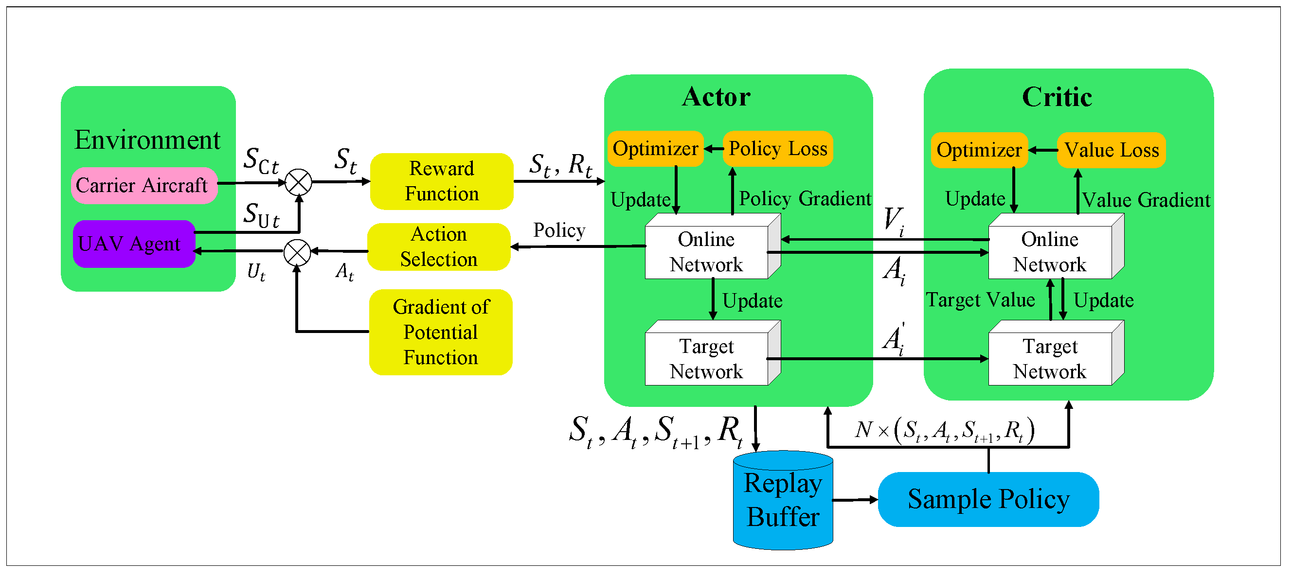
In PRL, the deep neural network for Q θ and π χ is called “critic” and “actor”, respectively. The entire algorithm training process is shown in Figure 9, and the training process will be performed offline. At each time step t + 1 , we collect the state s t , action a t , and reward R t from theast step and the current state s t + 1 , which will be stored as a tuple ( s t , a t , R t , s t + 1 ) at the replay buffer D [45]. At each step of policy evaluation or improvement, we randomly select a batch of historical data B from the replay buffer D to train the parameters θ of Q θ ( · ) and parameters χ of π χ .
At the policy evaluation step, the parameters θ are obtained by minimizing the Bellman residual. Furthermore, we introduce a copy of the actor and critic networks to calculate target values, which can slowly change the goal value to improve the stability ofearning.
J Q ( θ ) = E ( s t , a t ) D [ 1 2 ( Q θ ( s t , a t ) Q ^ ( s t , a t ) ) 2 ]
with
Q ^ ( s t , a t ) = R t + δ Q θ ¯ δ η ln ( π χ )
in which θ ¯ is the parameter of the target critic network.
Parameter χ is updated by adaptive momentum-estimation technique, and Equation (19) can be rewritten as
J π ( χ ) = E ( s t , a t ) D [ η ln π χ Q θ ( s t , a t ) ]
Th equation used to update the temperature parameter η is given as
J η = E π [ η ln π ( s t | a t ) η H ¯ ]
in which H ¯ is target entropy. If training is done, optimal parameters will be output by Algorithm 1, where λ Q , λ π , λ α > 0 areearning rates and τ > 0 is constant scalar.
Algorithm 1 PRL control algorithm
Initialize parameters θ , η and χ
     for all each iteration do
        for all each environment step do
             a t π χ ( a t | s t )
             s t + 1 P ( s t + 1 | s t , a t )
             D D { ( s t , a t , R t , s t + 1 ) }
        end for
        for all each gradient step do
            Sample a batch of data B from D
             θ θ λ Q ^ θ J Q ( θ )
             χ χ λ π ^ χ J π ( χ )
             η χ λ π ^ χ J π ( χ )
             θ ¯ τ θ + ( 1 τ ) θ ¯
        end for
     end for
     until training is done
     Output optimal parameters χ * , θ *

5. Performance Analysis

5.1. Converge Analysis

According to (21) and (25), R dis , R safe , and R sync are all non-positive. In addition, the reward function R done is bounded. Therefore, the total return R t is bounded, that is R t [ R min , R done ] , where R min is theowest bound of reward. For the convergence analysis of the PRL algorithm, the following Theorems 1 and 2 can be given.
Theorem 1.
Let T π be the Bellman backup operator under policy π , sequence Q i + 1 ( s , a ) = T π Q i ( s , a ) will coverage to Q-function Q π while i .
Proof. 
The specific proof process is detailed in Appendix A.
Theorem 2.
According to (18),et Q π old be the old policy π , it exists Q π old ( s , a ) Q π new ( s , a ) , s S and a A .
Proof. 
The specific proof process is detailed in Appendix B.
According to Theorems 1 and 2, the following theorem can be proposed, in which superscript k represents the result of the k -th iteration.
Theorem 3.
Suppose π k is the strategy obtained at the k -th iteration, if the strategy evaluation and improvement steps are applied repeatedly, there exists π k π o p t i m a l as k such that Q π o p t i m a l ( s , a ) Q π new ( s , a ) , s S and a A , where π o p t i m a l is the optimal policy.
Proof. 
The specific proof process is detailed in Appendix C.

5.2. Stability Analysis

According to the following theorem, there is stability of the PRL algorithm in the closed-loop tracking system.
Theorem 4.
To prove that the closed-loop tracking system is stable, the Q-functionearned in the PRL training process needs to satisfy.
ξ 1 R t Q π ( s , a ) ξ 2 R t
E s t ζ π [ E s t + 1 P π [ Q π ( s + 1 , a + 1 ) ] Q π ( s , a ) ] υ E s t ζ π [ R t ]
E s t ζ π [ s t ] ϵ t ξ 1 ξ 2 E s 0 ζ π [ s 0 ]
where ξ 1 > 0 , ξ 2 > 0 , υ > 0 , and ϵ ( 0 , 1 ) . ζ π ( s t ) can be expressed as
ζ π ( s t ) lim T 1 T t = 0 T P ( s t π , t )
Proof. 
The specific proof process is detailed in Appendix D.

6. Simulations and Comparisons

The numerical simulation results demonstrate the effectiveness of the proposed method in solving the rendezvous problem in UAV aerial recovery. First, the convergence and accuracy of the PRL algorithm were verified in a task scenario in which the recovery drogue moved along a straightine. Then, the algorithm was extended to a more complex rendezvous situation, in which the recovery drogue moved along a circle, and the performance of the proposed method was further investigated. The APF method, which enables real-time on-board execution [46,47], was used to solve this rendezvous problem with non-convex constraints for comparison [15,48] to demonstrate the performance of the PRL. Recycling in our simulation was considered successful if the following conditions were met:
d D t < 0.3 e v < 0.1
Note that l U l C > 0 should be satisfied at every step during the entire approach; otherwise, it is regarded as a failure.
Reinforcementearning training was conducted in an offline environment. In the actual simulation process, a real-time response can be achieved after the network parameters areoaded. In the modeling of safety constraints, the coordinates of the safety boundary control points N a established in the symmetric plane relative to the carrier after being converted to the the Cartesian coordinate system are given as N 0 ( 10 , 10 ) , N 1 ( 80 , 15 ) , N 2 ( 120 , 3 ) , N 3 ( 80 , 15 ) , N 4 ( 2 , 15 ) , N 5 ( 30 , 15 ) , N 6 ( 30 , 4 ) , N 7 ( 30 , 15 ) , N 8 ( 2 , 15 ) , N 9 ( 8 , 13 ) , and D 0 ( 15 , 15 ) . Table 1 summarizes the hyperparameters used in reinforcementearning. In combination with Algorithm 1, a training architecture of reinforcementearning was established.

6.1. Rendezvous on Straight-Line Path

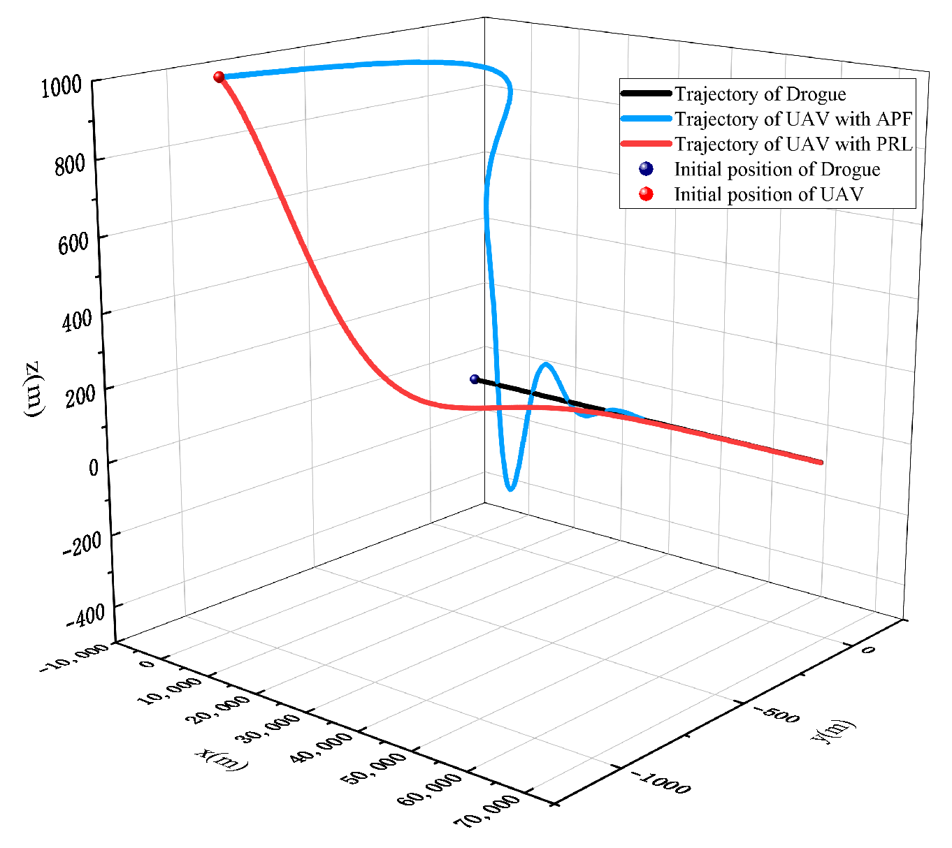
In the first case, the carrier plane is assumed to move along the x -direction at a constant speed of 161 m/s and the UAV approaches from above with an initial position deviation d D 0 = [ 1000 , 1000 , 1000 ] and initial speed e v 0 = [ 80 , 0 , 0 ] . Figure 10 shows the global trajectories of the different methods with the same initial state. Figure 11 shows the converged solutions for e x , e y , e z , v U t , e γ , e ψ . The red curves represent the solution obtained by the PRL, the blue curves represent the solution obtained by the APF, and the black dashedine represents the desired state curve.
As shown in Figure 11a, the position deviation in the x -direction always decreases throughout the process, and the APF converges faster in this direction. According to Figure 11b,c, in the y and z directions, the position deviation of the PRL in the direction steadily decreases, whereas the position deviation of the APF oscillatingly decreases. After a period, the relative position converges to a small value, and rendezvous occurs. Figure 11d shows that the overshoot of PRL was significantly smaller than that of APF as the ground speed approached the target value. Figure 11e,f shows that the velocity direction deviation of PRL quickly converged to the target value, whereas APF slowly converged. Combined with the global trajectory shown in Figure 10, both algorithms can generate trajectories that bring the drone closer to the target. Table 2 presents a comparison of the numerical results, which shows the average of 100 experiments of the two algorithms in random initial state, where the probability of reaching the allowable deviation range under the condition of satisfying the safety constraints is P suc . Based on the table, both methods can bring the UAV close to the target point, and the ending accuracy of Safe-RL is slightly higher.

6.2. Rendezvous on Circular Path

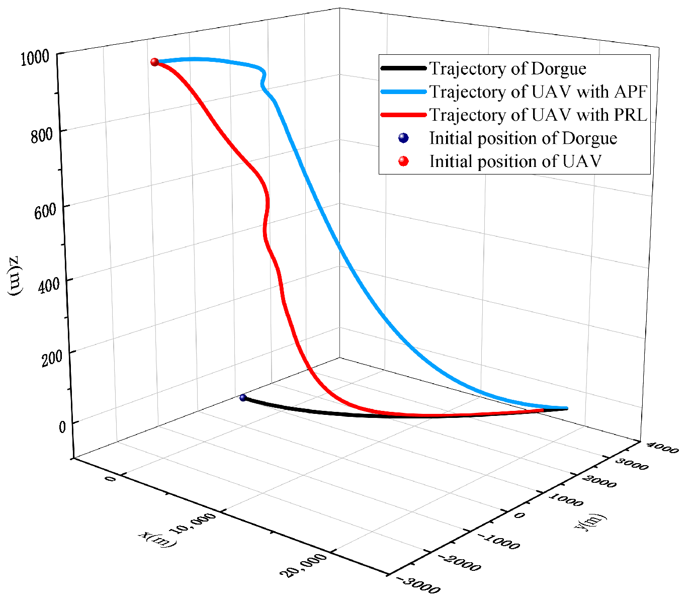
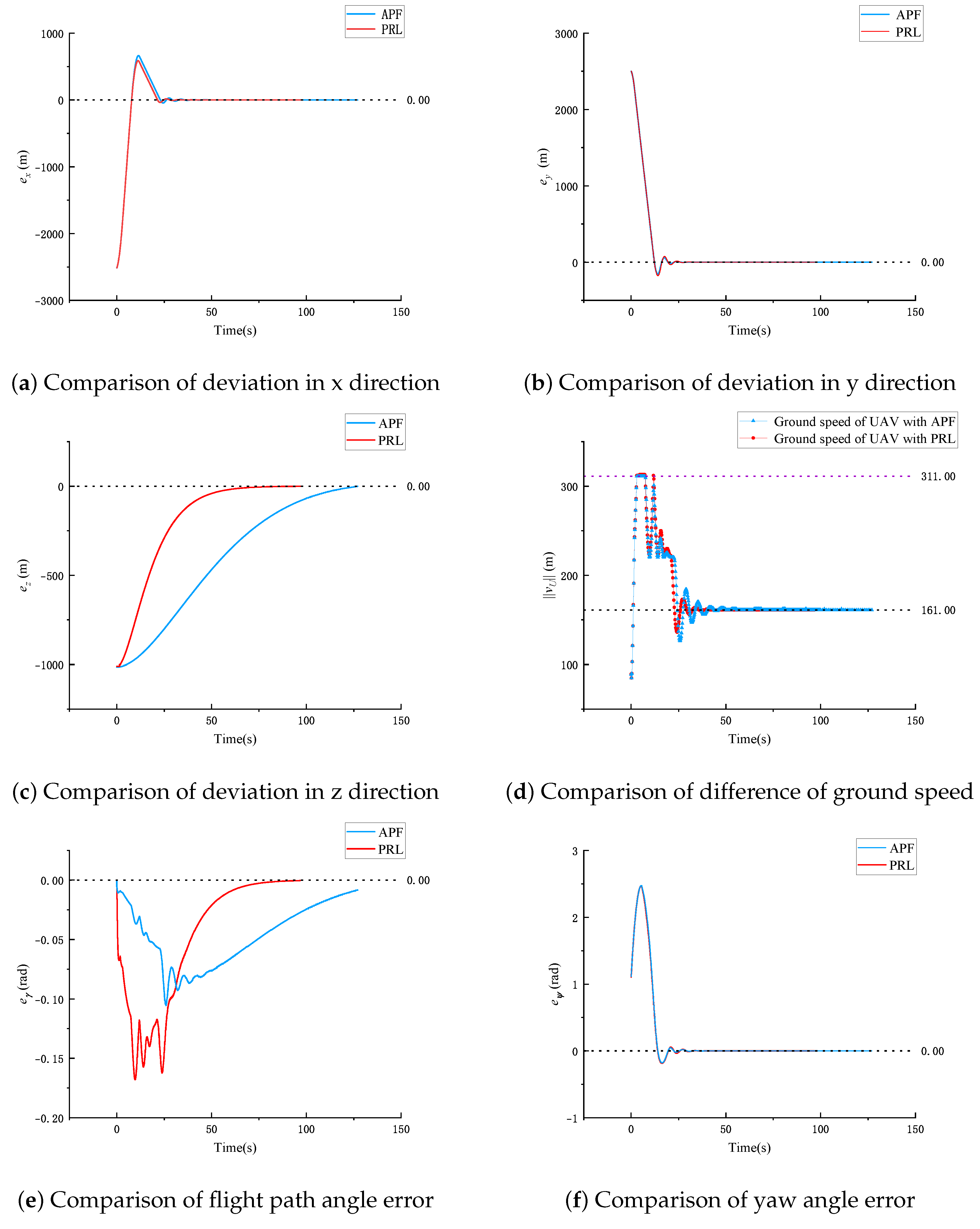
We consider a recovery drogue moving along a circular path in another intersection case, which is more complex than the straight-line intersection problem discussed in the previous subsection, to further investigate the performance of the proposed method. In this case, the speed of recovery of the drogue was 161 m/s, and the path radius was 72,000 m. The UAV approaches from above with an initial position deviation d D 0 = [ 2500 , 2500 , 1000 ] and initial speed e v 0 = [ 80 , 40 , 0 ] . Figure 12 shows the global trajectories of the different methods with the same initial state. In these cases, the PRL method provides a smoother trajectory than the APF. Figure 13 shows the converged solutions for e x , e y , e z , v U t , e γ , e ψ . The red curves represent the solution obtained by the PRL, the blue curves are the solution from APF, the black dashedine represents the desired state curve, and the purple dashedine indicates the upper bound of the control.
Based on the same parameter training used in Section 6.1, the PRL algorithm is implemented and the results are given as follows. Compared with the APF, similar to the solution observed in the previous example, the converged solutions of the two do not completely overlap; however, they follow a similar trend: the speed of the UAV reaches its upper bound at the beginning of the flight, as shown in Figure 11d, and hardly touches theower bound. As shown in Figure 11a–c, during the entire process, the position deviation continued to converge, and the PRL converged faster in the z direction. Figure 11e,f shows that at the end of the mission, the speed of the UAV obtained by the PRL algorithm is aligned with the heading direction of the recovery drogue, whereas the results of the APF algorithm still have a certain deviation, although the deviation isess than 0.01 rad. The 3D intersection trajectory shown in Figure 12 indicates that the recovery drogue completed a circular arc before the intersection occurred. Similarly, the PRL method provides a smoother trajectory than the APF. Table 3 presents the comparison of the numerical results; it shows the average of 100 experiments of the two algorithms in the same random initial state. The recovery success rate of the PRL was significantly higher than that of the APF. Section 6.3 analyzes the safety of the recovery process.

6.3. Security Analysis

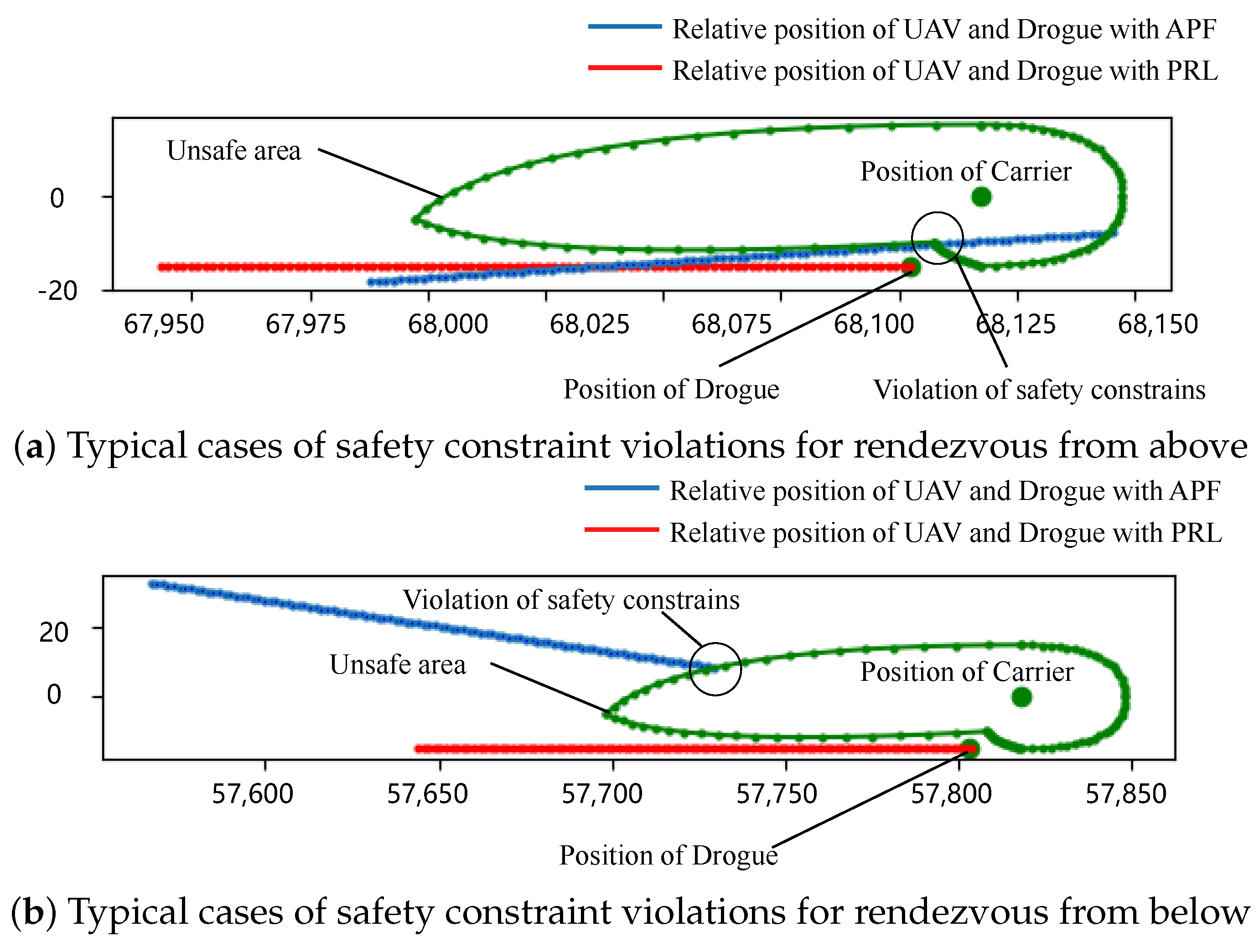
The comparisons of the success rates of PRL and APF are shown in Table 2 and Table 3. The success rate is the rate at which the UAV does not violate safety constraints and satisfies reachability. The results shown in the table prove the ability of PRL to solve the intersection problem with security constraints. Figure 14a shows typical cases of an approaching process with safety constraint violations of APF. Under the same initial state, the APF violates the safe constrains and breaks into the unsafe area, which frequently occurs in our test of 100 randomly initial states. This is because of the overshoot of the APF whose trajectory is not as smooth as PRL, which also causes it to touch the safety boundary at some point. Only when the trajectory is relatively flat can the target position be reached while ensuring safety. However, after training, owing to the penalty of security constraints, PRL has a significantly higher probability of satisfying reachability without violating the security constraints.
The results of the comprehensive simulation experiments can be used to easily compare the advantages of the proposed safe-RL algorithm. First, the convergence of PRL hasess overshoot and is more stable than APF. Second, PRL has a smaller terminal deviation. Finally, under the condition of satisfying the safety constraints, the task success rate of PRL is higher. In summary, the online feasible trajectory generation method has significant application potential for aerial recovery tasks.

7. Conclusions

To address a keyimitation in the current use of UAVs, this study considers rendezvous and docking problems based on aerial recovery. The main contributions of this study are as follows. First, a method of establishing safety constraints based on finite element analysis was proposed to model the non-safety region. Second, a reinforcementearning method based on a potential function was proposed to realize UAV online trajectory generation, while the trajectory satisfies the requirements of non-convex safety constraints. Finally, a reward function was designed such that the UAV can overcome the problem of reward sparsity even without expert experience. The simulation experiment results show that the performance of this algorithm is better than APF. The proposed algorithm has a smoother trajectory, higher efficiency, and can get closer to the targetocation. In terms of more important safety, in the two working conditions of the experiment, the success rates of this algorithm in avoiding hazard areas reached 100 % and 99 % , respectively, while APF was only 43 % and 33 % . Therefore, the proposed algorithm can be generalized to the rendezvous and docking problem as a baseline technology, demonstrating that autonomous real-time, collision-free rendezvous and aircraft approaches are feasible.

Author Contributions

Conceptualization, B.Z. and M.H.; methodology, B.Z. and M.H.; software, B.Z. and M.H.; validation, B.Z., M.H. and N.Q.; formal analysis, J.W. and B.Z.; investigation, B.Z., Z.Y. and J.W.; resources, N.Q.; data curation, B.Z. and Z.Y.; writing—original draft preparation, B.Z. and M.H.; writing—review and editing, B.Z., Z.Y. and N.Q.; visualization M.H. and J.W.; supervision, N.Q. and M.H.; project administration, N.Q.; funding acquisition, N.Q. and M.H. All authors have read and agreed to the published version of the manuscript.

Funding

This work was supported in part by the National Natural Science Foundation of China (grant number 12272104) and in part by the National Natural Science Foundation of China (grant number U22B2013).

Data Availability Statement

Data are contained within the article.

Conflicts of Interest

The authors declare no conflict of interest.

Appendix A. Proof of Theorem 1

Proof. 
First, define an entropy-enhanced reward R t ^ = R t δ E s t + 1 E π [ η ln ( π ( a t + 1 | s t + 1 ) ) ] which is bounded, the Bellman operation can be expressed as
T π Q π ( s , a ) = R t ^ + δ E s t + 1 [ Q π ( a t + 1 | s t + 1 ) ]
in terms of (16), Q π ( s , a ) = R t ^ + δ t + 1 a t + 1 π ( a t + 1 | s t + 1 ) s t + 1 P t + 1 | t R t + 1 ^ , so
Q π ( s t , a t ) R ¯ / ( 1 δ )
where Q π ( s t , a t ) = max s , a | Q π ( s t , a t ) | . Thus, Q π is bounded in -norm. There exists
T π Q π 1 T π Q π 2 = R t ^ + δ E s t + 1 [ Q π 1 ( a t + 1 | s t + 1 ) ] R t ^ δ E s t + 1 [ Q π 2 ( a t + 1 | s t + 1 ) ] δ Q π 1 Q π 2
where Q π 2 and Q π 1 are the Q-value atast and current iteration, respectively. Thus, lim i Q i + 1 ( s t , a t ) Q π .

Appendix B. Proof of Theorem 2

Proof. 
According to (18),
E π new [ η ln ( π ( a t | s t ) ) Q π old ( s t , a t ) ] E π old [ η ln ( π ( a t | s t ) ) Q π old ( s t , a t ) ]
combined with (A3), it can be derived that
Q π old ( s t , a t ) R t + δ E s t + 1 [ E π new [ R t + 1 + δ E s t + 2 [ E π new [ Q π old ( s t + 2 , a t + 2 ) δ ln π new ( a t + 2 | s t + 2 ) ] ] δ ln π new ( a t + 1 | s t + 1 ) ] ] Q π new ( s t , a t )

Appendix C. Proof of Theorem 3

Proof. 
According to (2), Q π ( s , a ) is monotonically non-decreasing as the number of policy network iteration steps increases, which means it will converge to its upper bound Q π * ( s , a ) with Q π * ( s , a ) Q π ( s , a ) s S and a A .

Appendix D. Proof of Theorem 4

Proof. 
The probability distribution of MDP under a strategy function p π ( s t ) = lim t P ( s t π , t ) . (32) can be rewritted as
S lim T 1 T t = 0 T P ( s t π , t ) × ( S P π ( s t + 1 | s t ) × Q t + 1 d s t + 1 Q t ) d s t = lim T 1 T t = 0 T ( E P ( s t + 1 | π , t + 1 ) [ Q t + 1 ] E P ( s t | π , t ) [ Q t ] )
Due to the variable ϵ always exists
( 1 ϵ 1 ) ξ 2 υ ϵ = 0
Combined with (32), it comes to
1 ϵ t + 1 E P ( s t + 1 π , t + 1 ) [ Q t + 1 ] 1 ϵ t E P ( s t π , t ) [ Q t ] 1 ϵ t ( ( 1 ϵ 1 ) ξ 2 υ ϵ ) R t
Thus,
1 ϵ t E P ( s t π , t ) [ Q t ] E P ( s 0 π , 0 ) [ Q 0 ] 0
From the above conclusions, we can get
E s t ζ π [ s t ] ϵ t ξ 2 ξ 1 E s 0 ζ π [ s 0 ]
The results show that the PRL algorithm can guarantee the exponential stability.

References

  1. Husseini, T. Gremlins are coming: Darpa enters phase III of its UAV programme. Army Technology, 3 July 2018. [Google Scholar]
  2. Nichols, J.W.; Sun, L.; Beard, R.W.; McLain, T. Aerial rendezvous of small unmanned aircraft using a passive towed cable system. J. Guid. Control. Dyn. 2014, 37, 1131–1142. [Google Scholar] [CrossRef]
  3. Hochstetler, R.D.; Bosma, J.; Chachad, G.; Blanken, M.L. Lighter-than-air (LTA) “airstation”—Unmanned aircraft system (UAS) carrier concept. In Proceedings of the 16th AIAA Aviation Technology, Integration, and Operations Conference, Washington, DC, USA, 13–17 July 2016; p. 4223. [Google Scholar]
  4. Wang, Y.; Wang, H.; Liu, B.; Liu, Y.; Wu, J.; Lu, Z. A visual navigation framework for the aerial recovery of UAVs. IEEE Trans. Instrum. Meas. 2021, 70, 5019713. [Google Scholar] [CrossRef]
  5. Darpa NABS Gremlin Drone in Midair for First Time. 2021. Available online: https://www.defensenews.com/unmanned (accessed on 1 July 2023).
  6. Gremlins Program Demonstrates Airborne Recovery. 2021. Available online: https://www.darpa.mil/news-events/2021-11-05 (accessed on 1 July 2023).
  7. Economon, T. Effects of wake vortices on commercial aircraft. In Proceedings of the 46th AIAA Aerospace Sciences Meeting and Exhibit, Reno, NV, USA, 7–10 January 2008; p. 1428. [Google Scholar]
  8. Wei, Z.; Li, X.; Liu, F. Research on aircraft wake vortex evolution and wake encounter in upper airspace. Int. J. Aeronaut. Space Sci. 2022, 23, 406–418. [Google Scholar] [CrossRef]
  9. Ruhland, J.; Heckmeier, F.M.; Breitsamter, C. Experimental and numerical analysis of wake vortex evolution behind transport aircraft with oscillating flaps. Aerosp. Sci. Technol. 2021, 119, 107163. [Google Scholar] [CrossRef]
  10. Visscher, I.D.; Lonfils, T.; Winckelmans, G. Fast-time modeling of ground effects on wake vortex transport and decay. J. Aircr. 2013, 50, 1514–1525. [Google Scholar] [CrossRef]
  11. Ahmad, N.N. Numerical simulation of the aircraft wake vortex flowfield. In Proceedings of the 5th AIAA Atmospheric and Space Environments Conference, San Diego, CA, USA, 24–27 June 2013; p. 2552. [Google Scholar]
  12. Misaka, T.; Holzäpfel, F.; Gerz, T. Large-eddy simulation of aircraft wake evolution from roll-up until vortex decay. AIAA J. 2015, 53, 2646–2670. [Google Scholar] [CrossRef]
  13. Liu, Y.; Qi, N.; Yao, W.; Zhao, J.; Xu, S. Cooperative path planning for aerial recovery of a UAV swarm using genetic algorithm and homotopic approach. Appl. Sci. 2020, 10, 4154. [Google Scholar] [CrossRef]
  14. Luo, D.; Xie, R.; Duan, H. A guidanceaw for UAV autonomous aerial refueling based on the iterative computation method. Chin. J. Aeronaut. 2014, 27, 875–883. [Google Scholar] [CrossRef]
  15. Zappulla, R.; Park, H.; Virgili-Llop, J.; Romano, M. Real-time autonomous spacecraft proximity maneuvers and docking using an adaptive artificial potential field approach. IEEE Trans. Control. Syst. Technol. 2018, 27, 2598–2605. [Google Scholar] [CrossRef]
  16. Shao, X.; Xia, Y.; Mei, Z.; Zhang, W. Model-guided reinforcementearning enclosing for UAVS with collision-free and reinforced tracking capability. Aerosp. Sci. Technol. 2023, 142, 108609. [Google Scholar] [CrossRef]
  17. Kim, S.-H.; Padilla, G.E.G.; Kim, K.-J.; Yu, K.-H. Flight path planning for a solar powered UAV in wind fields using direct collocation. IEEE Trans. Aerosp. Electron. Syst. 2019, 56, 1094–1105. [Google Scholar] [CrossRef]
  18. Bonalli, R.; Hérissé, B.; Trélat, E. Optimal control of endoatmosphericaunch vehicle systems: Geometric and computational issues. IEEE Trans. Autom. Control. 2019, 65, 2418–2433. [Google Scholar] [CrossRef]
  19. Shi, B.; Zhang, Y.; Mu, L.; Huang, J.; Xin, J.; Yi, Y.; Jiao, S.; Xie, G.; Liu, H. UAV trajectory generation based on integration of RRT and minimum snap algorithms. In Proceedings of the 2020 Chinese Automation Congress (CAC), Shanghai, China, 6–8 November 2020; IEEE: Piscataway, NJ, USA, 2020; pp. 4227–4232. [Google Scholar]
  20. Wang, Z.; Lu, Y. Improved sequential convex programming algorithms for entry trajectory optimization. J. Spacecr. Rocket. 2020, 57, 1373–1386. [Google Scholar] [CrossRef]
  21. Romano, M.; Friedman, D.A.; Shay, T.J. Laboratory experimentation of autonomous spacecraft approach and docking to a collaborative target. J. Spacecr. Rocket. 2017, 44, 164–173. [Google Scholar] [CrossRef]
  22. Fields, A.R. Continuous Control Artificial Potential Function Methods and Optimal Control. Master’s Thesis, Air Force Institute of Technology, Wright-Patterson, OH, USA, 2014. [Google Scholar]
  23. Lu, P.; Liu, X. Autonomous trajectory planning for rendezvous and proximity operations by conic optimization. J. Guid. Control. Dyn. 2013, 36, 375–389. [Google Scholar] [CrossRef]
  24. Virgili-Llop, J.; Zagaris, C.; Park, H.; Zappulla, R.; Romano, M. Experimental evaluation of model predictive control and inverse dynamics control for spacecraft proximity and docking maneuvers. CEAS Space J. 2018, 10, 37–49. [Google Scholar] [CrossRef]
  25. Sun, L.; Huo, W.; Jiao, Z. Adaptive backstepping control of spacecraft rendezvous and proximity operations with input saturation and full-state constraint. IEEE Trans. Ind. Electron. 2016, 64, 480–492. [Google Scholar] [CrossRef]
  26. Faust, A.; Oslund, K.; Ramirez, O.; Francis, A.; Tapia, L.; Fiser, M.; Davidson, J. PRM-RL: Long-range robotic navigation tasks by combining reinforcement earning and sampling-based planning. In Proceedings of the 2018 IEEE International Conference on Robotics and Automation (ICRA), Brisbane, Australia, 21–25 May 2018; IEEE: Piscataway, NJ, USA, 2018; pp. 5113–5120. [Google Scholar]
  27. Williams, K.R.; Schlossman, R.; Whitten, D.; Ingram, J.; Musuvathy, S.; Pagan, J.; Williams, K.A.; Green, S.; Patel, A.; Mazumdar, A.; et al. Trajectory planning with deep reinforcementearning in high-level action spaces. IEEE Trans. Aerosp. Electron. Syst. 2022, 59, 2513–2529. [Google Scholar] [CrossRef]
  28. Dhuheir, M.; Baccour, E.; Erbad, A.; Al-Obaidi, S.S.; Hamdi, M. Deep reinforcement earning for trajectory path planning and distributed inference in resource-constrained UAV swarms. IEEE Internet Things J. 2022, 10, 8185–8201. [Google Scholar] [CrossRef]
  29. Song, Y.; Romero, A.; Müller, M.; Koltun, V.; Scaramuzza, D. Reaching theimit in autonomous racing: Optimal control versus reinforcementearning. Sci. Robot. 2023, 8, eadg1462. [Google Scholar] [CrossRef]
  30. Bellemare, M.G.; Candido, S.; Castro, P.S.; Gong, J.; Machado, M.C.; Moitra, S.; Ponda, S.S.; Wang, Z. Autonomous navigation of stratospheric balloons using reinforcementearning. Nature 2020, 588, 77–82. [Google Scholar] [CrossRef]
  31. Zhang, H.; Zongxia, J.; Shang, Y.; Xiaochao, L.; Pengyuan, Q.; Shuai, W. Ground maneuver for front-wheel drive aircraft via deep reinforcementearning. Chin. J. Aeronaut. 2021, 34, 166–176. [Google Scholar] [CrossRef]
  32. Wang, C.; Wang, J.; Wang, J.; Zhang, X. Deep-reinforcement-learning-based autonomous uav navigation with sparse rewards. IEEE Internet Things J. 2020, 7, 6180–6190. [Google Scholar] [CrossRef]
  33. Burda, Y.; Edwards, H.; Pathak, D.; Storkey, A.; Darrell, T.; Efros, A.A. Large-scale study of curiosity-drivenearning. arXiv 2018, arXiv:1808.04355. [Google Scholar]
  34. Pathak, D.; Agrawal, P.; Efros, A.A.; Darrell, T. Curiosity-driven exploration by self-supervised prediction. In Proceedings of the International Conference on Machine Learning, PMLR, Sydney, Australia, 6–1 August 2017; pp. 2778–2787. [Google Scholar]
  35. Houthooft, R.; Chen, X.; Duan, Y.; Schulman, J.; Turck, F.D.; Abbeel, P. VIME: Variational information maximizing exploration. Adv. Neural Inf. Process. Syst. 2016, 29, 1–9. [Google Scholar] [CrossRef]
  36. Ng, A.Y.; Harada, D.; Russell, S. Policy invariance under reward transformations: Theory and application to reward shaping. In Proceedings of the ICML, Bled, Slovenia, 27–30 June 1999; Volume 99, pp. 278–287. [Google Scholar]
  37. Yan, C.; Xiang, X.; Wang, C.; Li, F.; Wang, X.; Xu, X.; Shen, L. Pascal: Population-specific curriculum-based madrl for collision-free flocking with arge-scale fixed-wing UAV swarms. Aerosp. Sci. Technol. 2023, 133, 108091. [Google Scholar] [CrossRef]
  38. Schwarz, C.W.; Hahn, K.-U. Full-flight simulator study for wake vortex hazard area investigation. Aerosp. Sci. Technol. 2006, 10, 136–143. [Google Scholar] [CrossRef]
  39. Rossow, V.J. Validation of vortex-lattice method foroads on wings in ift-generated wakes. J. Aircr. 1995, 32, 1254–1262. [Google Scholar] [CrossRef]
  40. Schwarz, C.; Hahn, K.-U. Gefährdung beim einfliegen von wirbelschleppen. In Proceedings of the Deutscher Luft- und Raumfahrtkongress 2003, Jahrbuch 2003, Munich, Germany, 17–20 November 2003. [Google Scholar]
  41. Munoz, J.; Boyarko, G.; Fitz-Coy, N. Rapid path-planning options for autonomous proximity operations of spacecraft. In Proceedings of the AIAA/AAS Astrodynamics Specialist Conference, Toronto, ON, Canada, 2–5 August 2010; p. 7667. [Google Scholar]
  42. Haarnoja, T.; Zhou, A.; Abbeel, P.; Levine, S. Soft actor-critic: Off-policy maximum entropy deep reinforcementearning with a stochastic actor. In Proceedings of the International Conference on Machine Learning, PMLR, Vienna, Austria, 25–31 July 2018; pp. 1861–1870. [Google Scholar]
  43. Zhang, Q.; Pan, W.; Reppa, V. Model-reference reinforcementearning for collision-free tracking control of autonomous surface vehicles. IEEE Trans. Intell. Transp. Syst. 2021, 23, 8770–8781. [Google Scholar] [CrossRef]
  44. Qi, C.; Wu, C.; Lei, L.; Li, X.; Cong, P. UAV path planning based on the improved ppo algorithm. In Proceedings of the 2022 Asia Conference on Advanced Robotics, Automation, and Control Engineering (ARACE), Qingdao, China, 26–28 August 2022; IEEE: Piscataway, NJ, USA, 2022; pp. 193–199. [Google Scholar]
  45. Mnih, V.; Kavukcuoglu, K.; Silver, D.; Rusu, A.A.; Veness, J.; Bellemare, M.G.; Graves, A.; Riedmiller, M.; Fidjeland, A.K.; Ostrovski, G.; et al. Human-level control through deep reinforcementearning. Nature 2015, 518, 529–533. [Google Scholar] [CrossRef] [PubMed]
  46. Munoz, J.D. Rapid Path-Planning Algorithms for Autonomous Proximity Operations of Satellites. Ph.D. Thesis, University of Florida, Gainesville, FL, USA, 2011. [Google Scholar]
  47. Bevilacqua, R.; Lehmann, T.; Romano, M. Development and experimentation of LQR/APF guidance and control for autonomous proximity maneuvers of multiple spacecraft. Acta Astronaut. 2011, 68, 1260–1275. [Google Scholar] [CrossRef]
  48. Lopez, I.; Mclnnes, C.R. Autonomous rendezvous using artificial potential function guidance. J. Guid. Control. Dyn. 1995, 18, 237–241. [Google Scholar] [CrossRef]
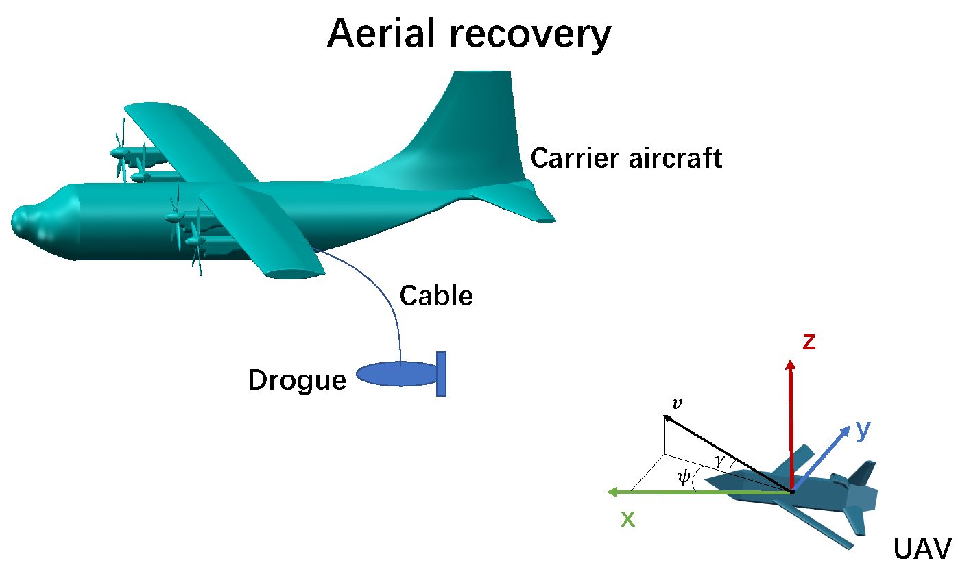
Figure 1. Schematic diagram of UAV aerial recovery.
Aerospace 11 00027 g001
Figure 2. Model of Carrier Aircraft.
Aerospace 11 00027 g002
Figure 3. Meshing results.
Aerospace 11 00027 g003
Figure 4. Vortex core region. Velocity is defined using the vorticity method in (a) and the velocity swirling strength is defined using the swirling method in (b).
Aerospace 11 00027 g004
Figure 5. Velocity and pressure distribution cloud map on the side view.
Aerospace 11 00027 g005
Figure 6. Cloud map of wake vorticity.
Aerospace 11 00027 g006
Figure 7. Tangential velocity vector diagram of vortex with different flow field sections. (a) Velocity vector diagram of flow field section at 30 m behind the wing; (b) velocity vector diagram of flow field section at 50 m behind the wing.
Aerospace 11 00027 g007
Figure 8. Safety constrains for Aerial Recovery, where N 0 ( N 10 ), N 2 , N 4 , N 6 , N 8 are the points farthest from the carrier aircraft in this area, respectively; A 0 is the intersection point of the ray in this direction and the contourine.
Aerospace 11 00027 g008
Figure 9. Implementation of the PRL control algorithm.
Aerospace 11 00027 g009
Figure 10. Global trajectory of aerial recovery of Case 1.
Aerospace 11 00027 g010
Figure 11. Converged solution results of Case 1.
Aerospace 11 00027 g011
Figure 12. Global trajectory of aerial recovery of Case 2.
Aerospace 11 00027 g012
Figure 13. Converged solution results of Case 2.
Aerospace 11 00027 g013
Figure 14. Typical cases of the terminal trajectory of PRL and APF.
Aerospace 11 00027 g014
Table 1. Hyperparameters of PRL.
HyperparametersValue
Sample batchsize | B | 512
Learning rate μ π 1 × 10 3
Learning rate μ V 2 × 10 3
Discount factor δ 0.99
Neural network structure of policy(256, 256)
Neural network structure of Value(256, 256)
Time step (ms)10
ϵ 0.2
C R [50.0, 5.0, 20.0, 20.0]
Table 2. Comparison of average final state of rendezvousing on straight-line path.
MethodPRLAPF
d D t , m/s 1.47 × 10 1 1.93 × 10 1
v U , m/s 161 161
e γ , rad 3.5 × 10 15 9.98 × 10 4
e ψ , rad 5.7 × 10 40 8.07 × 10 4
P suc , Success rate 1.00 0.43
Table 3. Comparison of average final state of rendezvous on circular path.
MethodPRLAPF
d D t , m/s 1.97 × 10 1 2.22 × 10 1
v U , m/s 161 161
e γ , rad 1.00 × 10 5 1.79 × 10 3
e ψ , rad 3.91 × 10 4 8.07 × 10 3
P suc , Success rate 0.99 0.33
Disclaimer/Publisher’s Note: The statements, opinions and data contained in all publications are solely those of the individual author(s) and contributor(s) and not of MDPI and/or the editor(s). MDPI and/or the editor(s) disclaim responsibility for any injury to people or property resulting from any ideas, methods, instructions or products referred to in the content.