Abstract
In this paper, an adaptive neural network global fractional order fast terminal sliding mode model-free intelligent PID control strategy (termed as TDE-ANNGFOFTSMC-MFIPIDC) is proposed for the hypersonic vehicle ground thermal environment simulation test device (GTESTD). Firstly, the mathematical model of the GTESTD is transformed into an ultra-local model to ensure that the control strategy design process does not rely on the potentially inaccurate dynamic GTESTD model. Meanwhile, time delay estimation (TDE) is employed to estimate the unknown terms of the ultra-local model. Next, a global fractional-order fast terminal sliding mode surface (GFOFTSMS) is introduced to effectively reduce the estimation error generated by TDE. It also eliminates arrival time, accelerates the convergence speed of the sliding phase, guarantees finite time arrival, avoids the singularity phenomenon, and bolsters robustness. Then, as the upper bound of the disturbance error is unknown, an adaptive neural network (ANN) control is designed to approximate the upper bound of the estimation error closely and mitigate the chattering phenomenon. Furthermore, the stability of the control system and the convergence time are proven by the Lyapunov stability theorem and are calculated, respectively. Finally, simulation results are conducted to validate the efficacy of the proposed control strategy.
1. Introduction
For hypersonic vehicles (HV) flying at high Mach numbers [1], the surrounding airflow compresses against and generates friction with their surfaces. This leads to the rapid generation of immense thermal energy, causing a sudden surge in the HV’s surface temperature—a phenomenon known as “aerodynamic heating” [2]. This intense aerodynamic heating, often referred to as the “thermal barrier” problem, can compromise flight stability, diminish the structural integrity of the HV, reduce the material’s strength limit, and potentially jeopardize the stability and reliability of the internal sophisticated electronic components.
To comprehensively address the challenging “thermal barrier” problem and validate the effectiveness of various insulation materials, scholars have turned to the advanced Ground Thermal Environment Simulation Test Device (GTESTD). This innovative device is meticulously designed to closely and accurately replicate the intense thermal conditions that hypersonic vehicles (HVs) inevitably encounter during their high-speed trajectories. By doing so, it provides a reliable platform for assessing the performance and resilience of different materials within these harsh thermal environments. The feedback from these tests is invaluable, as it allows researchers and designers to make data-driven decisions, adjusting material choices and configurations to optimize their resistance to aerodynamic heating. The efficacy of GTESTD is intrinsically linked to its precision in mirroring the real-flight thermal environment, making its accuracy a cornerstone for ensuring the safe operation of HVs. Within this realm of simulation, the quartz lamp [3] has been recognized as a game-changer. Its rapid heating rate, formidable power and remarkably low thermal inertia have made it the go-to choice as the primary radiant heating element in these simulations. When incorporated into the GTESTD, quartz lamp heaters not only ensure effective and consistent thermal replication but also present a solution that is marked by their reduced technical challenges, cost-effectiveness and a considerably low associated risk factor. Furthermore, the versatility of GTESTD equipped with quartz lamp heaters is noteworthy. It stands out as the most suitable and reliable testing method, especially when dealing with scenarios that require simulation across multitemperature zones, those that are time-variant, or even comprehensive full-scale thermal examinations. This adaptability is essential, considering the complexities associated with the flight thermal environment of HVs. These vehicles operate in conditions characterized by their transience, extreme nonlinearity, and intricacies stemming from complex, strongly coupled variations in temperature and pressure. Despite the capabilities of GTESTD, a significant challenge persists. The control strategies governing the operation of GTESTD are still rooted in more traditional methodologies. While these methods have their merits, they often find themselves inadequately equipped to manage the intricate dynamics of hypersonic flight simulations, particularly when the need is for swift responses and high-precision dynamic control performance. This gap underscores the imperative need for continual innovation in control strategies, pushing the boundaries of what is possible to ensure the safety and reliability of future hypersonic flights.
Given the parametric uncertainties, internal input disturbances and external disturbances associated with GTESTD, constructing an accurate mathematical model proves challenging. While modern control theories such as adaptive control [4], model predictive control [5,6], and sliding mode control [7] are difficult to implement, advancements in control theory have led to the abstraction of some control methods from their respective mathematical models. Fliess and Join introduced the concept of model-free control (MFC) based on an ultra-local model [8,9], a method that does not hinge on the precise mathematical model of the system, but rather leverages its input and output. In a related work, Aneesh [10] presented a model-free intelligent PID control (MFIPIDC) strategy for the pitch and altitude control of flapping wing flying robots, mitigating errors stemming from flawed flapping dynamics or insufficient modeling. Given the merits of MFC rooted in the ultra-local model, MFC emerges as a promising alternative to the mathematical modeling of GTESTD.
The estimation of uncertainties and disturbances is a crucial facet of the ultra-local model and has been the subject of extensive discussion [11,12]. The time delay estimation (TDE) [13] technique stands out for its ability to measure and compensate for unknown terms, offering a straightforward implementation for estimating real-time uncertainties and external disturbances. Notably, TDE does not introduce any system delays. Owing to TDE’s inherent advantages, it has been widely adopted in various systems, including permanent magnet motors [14], lower limb exoskeletons [15] and tri-rotor unmanned aerial vehicles [16]. In [17,18], both the robotic arm and HVAC systems were governed by a model-free intelligent PID based on TDE (TDE-MFIPIDC). However, their tracking performances were only marginally enhanced due to the estimation errors inherent to TDE.
Given TDE’s estimation errors for overall disturbances and uncertainties, the TDE-MFIPIDC strategy can at best ensure a bounded tracking error without assurances of swift convergence to zero. To overcome this limitation, sliding mode control (SMC) and terminal sliding mode control (TSMC) strategies are amalgamated with TDE and MFC methodologies [19,20]. Beyond the attributes of SMC, TSMC offers finite-time convergence and a reduction in steady-state error. In [21], this paper presents finite-time event-triggered formation control for multiple quadrotor unmanned aerial vehicles (UAVs) in the presence of unknown external disturbances. Utilizing adaptive terminal sliding mode control methods, novel adaptive distributed, robust event-triggered controllers are introduced, achieving efficient control update, reduced chattering, and ensuring closed-loop signal stability. In [22], this study introduces a finite-time adaptive tracking control algorithm, rooted in nonsingular terminal sliding mode (NTSM), to address the consensus challenges in second-order multi-agent systems (MAS) subjected to disturbances. The method incorporates a finite-time disturbance observer using NTSM to estimate and offset the disturbance, and an NTSM adaptive controller is crafted to bolster system robustness, augment response swiftness, and enhance tracking precision. However, during the TSMC control process, challenges arise, including noticeable chattering during the reaching phase, slower convergence in the sliding phase, and potential singularity issues. In [23], a Global TSMC (GTSMC) strategy was introduced for missile system control. This strategy, particularly in the integral term design of the global terminal sliding mode surface (GTSMS), not only sidesteps the singularity issue but also ensures system states initiate within the sliding phase, eliminating the reaching phase duration. We then propose the integration of a fast term into GTSMS to accelerate the sliding phase’s convergence rate. The Fractional Order (FO) theory, which has garnered significant interest in recent years, has birthed numerous fractional-order controllers, like FOPID control [24], FOSMC [25], and FO adaptive control [20]. These controllers have outperformed their integer-order counterparts due to their adaptability in integration and differentiation processes. Consequently, this paper presents a Global Fractional Order Fast Terminal Sliding Mode Control (GFOFTSMC) strategy, drawing from the GTSMC approach, the fast term, and FO principles.
In most practical scenarios, the upper bound of estimation error remains elusive. The prevalent approach involves choosing a larger switching gain to encompass potential error values; however, this can lead to pronounced chattering. Recognizing the neural network’s capacity for infinite approximation, this study introduces an adaptive neural network (ANN) [26,27] control strategy. By approximating the switching gain, it aims to infinitely approach the unknown upper bound of the estimation error, thereby mitigating the chattering effect.
Drawing on the aforementioned research, this study introduces an adaptive neural network global fractional order fast terminal sliding mode model-free intelligent PID control strategy based on time delay estimation (TDE-ANNGFOFTSMC-MFIPIDC) for temperature regulation in GTESTD. The innovation of this research lies in the integration of the ultra-local model, IPID control, TDE technique, sliding mode control, adaptive control, and neural network control to govern uncertain systems. The ultra-local model serves as a substitute for imprecise mathematical models, while TDE estimates the unknown elements within this model. The IPID control, acting as the primary controller, ensures convergence within a finite timeframe. Sliding mode control, on the other hand, minimizes the estimation error introduced by TDE, eradicates arrival time delays, accelerates the convergence during the sliding phase, assures finite-time arrival, prevents the singularity phenomenon, and bolsters system robustness. Lastly, the ANN, grounded on the cubic B-spline function, is deployed to closely approximate the maximum bound of the estimation error, subsequently reducing the chattering effect. Therefore, the main contributions can be summarized as follows:
- (1)
- Our proposed control strategy is built upon the TDE framework, enhanced by GFOFTSMC to address estimation errors, and incorporates an ANN rooted in the cubic B-spline function for precise switching gain approximation. By sidestepping traditional mathematical models, this strategy offers both robustness and streamlined control performance.
- (2)
- IPID serves as the principal controller, significantly streamlining the parameter tuning process.
- (3)
- The sliding mode surface, formulated using GTSMS, fast term and FO, boasts features, such as the elimination of arrival time, expedited convergence in the sliding phase, assurance of finite-time arrival, singularity prevention and heightened robustness.
- (4)
- The system’s stability and finite-time calculations are underscored by the Lyapunov stability theorem and finite-time stability theorem, respectively.
The remainder of this paper unfolds as follows: Section 2 introduces the mathematical model of GTESTD. Section 3 delves into controller design and stability analysis, incorporating MFC, TDE, and the ANNGFOFTSMC strategy. Section 4 presents simulation data from the missile’s thermal environment and compares various control strategies. Finally, Section 5 offers concluding remarks on this research.
2. Mathematical Model and Preliminaries
2.1. Mathematical Model
As mentioned above, the surface temperature of HV is highly nonlinear and transient, and GTESTD is also a nonlinear system. In order to facilitate the design of control strategies and acquire the control performance of real thermal simulations, the mathematical model of GTESTD needs to be established [28].
As depicted in Figure 1, GTESTD consists of three primary components: the heating unit, the control unit, and the temperature measurement unit. The heating unit is structured using several sets of quartz lamp tubes, collectively forming a quartz lamp heater. By employing a power-adjusting device, the unit modifies the terminal voltage to regulate the output temperature. Meanwhile, the control unit directs the power adjusting device, adjusting the trigger of the conduction angle based on a specifically designed control strategy. The temperature measurement unit’s chief role is to offer real-time feedback on the heating unit’s output temperature. The heating unit establishes the mathematical model for GTESTD, with the essential symbols detailed in Table 1.
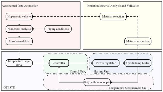
Figure 1.
Schema of the ground thermal environment simulation test device.

Table 1.
Description of essential symbols in the GTESTD model.
Assumption 1.
The heat generated by viscous dissipation and thermal expansion during heat transfer is ignored, only the internal energy absorbed by the quartz lamp filament and the energy lost by convection, heat conduction and thermal radiation are considered; the equation of electric heating energy is described as follows [29]:
According to the law of conservation of energy, the electric heating energy absorbed by quartz lamp ought to be equal to the power supplied to the quartz lamp by the power adjusting device, the expression is given as follows:
Substituting Formula (1) into Formula (2), then Formula (2) is further deduced, the mathematical model expression of GTESTD is as follows [30]:
where is the derivative of .
2.2. Preliminaries
Definition 1 [31].
The Riemann–Liouville th-order fractional integral of function is defined as follows:
Definition 2.
Riemann–Liouville fractional derivative, as the earliest fractional derivative with the most complete theoretical research, is defined as follows:
Lemma 1.
Fractional derivative and integral have the following properties:
Definition 3 [32].
Consider the nonlinear system , finite time stable needs to satisfy: (1) system is stable; (2) when the initial state , there exists
and ,
is guaranteed for any
Lemma 2 [27].
Consider the system . Define:
Then, the system is finite-time stable. The setting time which is limited by:
where is the initial value of , .
Lemma 3 [33].
The inequality satisfies:
Lemma 4 [34].
Consider a positive Lyapunov function
satisfied
for any real numbers
and , then the system convergences in finite time. The corresponding reaching time
is given by:
3. Control Strategy Development
This research focuses on tracking temperature in a time sequence. To accurately track the surface temperature of HV during flight, the MFIPIDC strategy based on GFOFTSMC, neural network adaptive law, and TDE is proposed. The design process is described as follows:
Step 1: Replacing the mathematical model of GTESTD with an ultra-local model to reduce orders in the dynamic model.
Step 2: Using TDE technique to estimate unknown disturbances and uncertainties in the system and compensate them into the ultra-local model.
Step 3: Using the method of combining GTSMS and fast term with FO, a sliding surface with the characteristics of eliminating arrival time, accelerating the convergence speed of the sliding phase, ensuring finite time arrival, avoiding singularity and enhancing robustness was developed.
Step 4: Employing ANN approximate switching gain based on the cubic B-spline function to infinitely approach the upper bound of estimation error and weaken the chattering phenomenon.
Step 5: Proving system stability based on the Lyapunov stability theorem and calculating finite time using the finite time stable theorem.
The designed control strategy structure block diagram is shown in Figure 2.
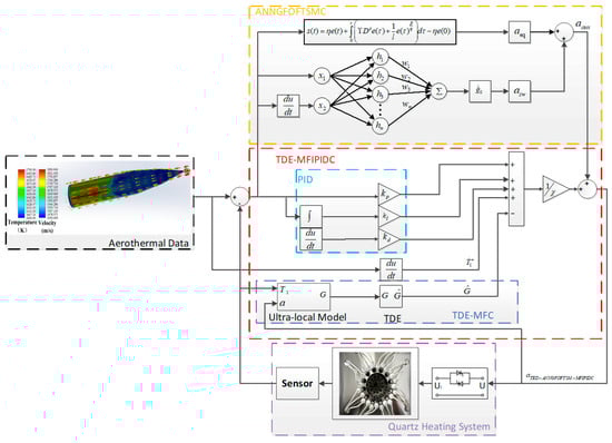
Figure 2.
Block diagram of our newly proposed TDE-ANNGFOFTSMC-MFIPIDC strategy.
3.1. Model-Free Control
Definition 4.
Consider a general implicit nonlinear system , an ultra-local model based on the idea of model-free control is simplified to a simple structure:
Assume that in Formula (14):
Considering that the trigonometric function of Formula (3) has distinct periodic oscillations and high-order terms are nonlinear, can be viewed as the sum of disturbances and they contain both the input disturbances and output disturbances. In view of being a first-order SISO system, the mathematical model of the GTESTD is transformed into the corresponding ultra-local model as [30]:
where and are the output and control input variables of GTESTD, respectively; the range of control input is ; is input gain, which is a nonphysical parameter and chosen by trails not predefined; , as the most important part of the ultra-local model, which includes internal uncertainties and external disturbances from local periodic oscillation () and high-order nonlinear output (); the value of is estimated by the measurements of and .
3.2. TED-MFIPIDC Strategy
The estimation of is a crucial issue for the effectiveness of MFC. Conventional estimation techniques, such as adaptive techniques and intelligent control, generally entail numerous parameters of the system model to obtain , which are not applicable to complex practical systems. The time delay estimation technique, as a simple, straightforward, and effective approach, is utilized to estimate the sum of disturbances, which does not cause time-delay phenomenon for the system [35].
The core concept behind the TDE technique is to use the control input, , and the system output, , measured from the previous instant, to estimate the combined effect of uncertainties and external disturbances in the current moment. This is achieved by introducing a slight delay interval, . While maintaining system stability, a smaller leads to a more precise estimation of disturbances.
Assumption 2.
is continuous and delay interval
is small enough. Then, based on TDE, the unknown term
can be approximated as:
The estimation error is defined:
where is the estimation error of .
Define:
where is the tracking error, is the output target temperature.
Assumption 3.
Output target temperature
is differentiable at all times,
is the differential of
with respect to time.
Then, both sides of Formula (20) are divided by :
where is the derivative of , is the derivative of The TDE-MFIPIDC strategy is defined as [8]:
where is the control law of the TDE-MFIPIDC strategy; , , and are adjustable parameters.
Substituting Formula (16) and (22) into (21), the error equation is calculated as:
Assumption 4.
The initial values of the estimation error and the tracking error are and 0, respectively.
Through Laplace transformation, combining Formula (23) and initial values, the following equation relationship can be derived:
Sequentially, according to the Final Value Theorem, the steady-state tracking error of Formula (25) is calculated as [36]:
From the above calculation results, it can be seen that the tracking error can converge to zero when the time goes to infinity. With the appropriate selection of , and , is just under bounded due to the time delay [37].
3.3. TDE-GFOFTSMC-MFIPIDC Strategy
To compensate the estimation error and obtain fast convergence, a new GFOFTSMC strategy combined with the TDE-MFIPIDC strategy is proposed. Together with the TDE-MFIPIDC strategy, the TDE-GFOFTSMC-MFIPIDC law is designed as follows:
where is the control law of the TDE-GFOFTSMC-MFIPIDC strategy; is the global fractional order fast terminal sliding auxiliary control law, , and are equivalent control law and switching control law, respectively; , , and are adjustable parameters.
Substituting Formula (16), (19) and (21) to (27), can be rewritten:
Based on the traditional GTSMS [23], a new global fractional-order fast terminal sliding mode surface (GFOFTSMS) is designed by introducing FO and fast term:
where is a fractional order, and are positive odd integers; , , and are all tuning gains; denotes the initial value of .
Sequentially, the derivative of Formula (30) is calculated as:
Substituting Formulas (13), (19) and (21) into Formula (31), Formula (31) can be written:
Under the condition of , the equivalent law of the TDE-GFOFTSMC-MFIPIDC strategy can be obtained as:
where , , and are adjustable parameters.
The purpose of switching the control law is to guarantee that when the system trajectory slides out of the sliding mode surface, it is forced to reach the sliding mode surface again to solve the convergence stagnation problem. The switching control rate needs to satisfy the sufficient stability condition [38]:
where is a positive constant.
Substituting Formulas (27), (32) and Formula (33) into Formula (35), Formula (35) can be written:
Then, Formula (36) is further calculated:
where .
Assumption 5 [39].
The absolute value of the TDE estimation error has the upper bound and satisfies the following condition:
According to Assumption 5, the maximum condition is satisfied; the inequality relationship in Formula (37) can be written as:
Subsequently, Formula (33) and Formula (40) are introduced into Formula (27), can be calculated as:
3.4. TDE-ANNGFOFTSMC-MFIPIDC Strategy
In the design of the above control strategy, two cases are considered: one is to directly determine the value of when the upper bound of the estimation error is known; the other is to select a sufficiently large upper bound to cover a wide range of uncertainties when the upper bound of the estimation error is unknown. Such a design will inevitably lead to excessive switching gain and chattering phenomena. Usually, in practical applications, it is difficult or impossible to obtain the value of . To solve this problem and further optimize the control strategy, an RBF neural network control law is introduced.
The RBF neural network structure is composed of an input layer, a hidden layer and an output layer, which is shown in Figure 3. The output of the RBF neural network can be determined as follows [27]:
where is the number of neurons in a single hidden layer; is the adjustable synaptic weight; is the RBF activation function; the input vector and RBF activation function center vector, respectively.
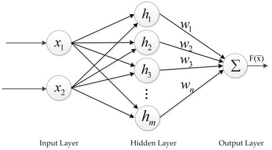
Figure 3.
The structure of RBF neural network.
For convenience, Formula (42) is further simplified as follows:
where is the weight matric.
The advantage of ANN is that after determining the number of neurons, their weights are adaptive and can adaptively adjust to the optimal weights. Therefore, no data is needed for training, testing and tuning.
According to Assumption 5, an RBF neural network adaptive law, as an approximate estimator, is utilized to approximate the upper bound of TDE estimation error by , which is designed as [27]:
where is the approximate value of ; is the designed control gain of the adaptive law and is a positive constant; is the activation function of the hidden layer; is the optimal weight of the weight from the hidden layer to the output layer, which should be satisfied with ; is the estimate value of ; is the adaptive law of ; is the approximate error between and .
Hidden layer activation function selects a cubic B-spline function, defined as:
where , Euclidean norm, is the distance between the input vector and the center vector, is the input vector, and are the center vector; is the width of the cubic B-spline function. They satisfy these conditions:
Eventually, by adding the neural network adaptive law, the TDE-ANNGFOFTSMC-MFIPIDC strategy is designed as:
where, is the control law of the TDE-ANNGFOFTSMC-MFIPIDC strategy.
3.5. Stability Analysis
Proof 1.
The stability of the TDE-ANNGFOFTSMC-MFIPIDC strategy is proved:
Define the Lyapunov function:
where , is the weight error, is the transpose of .
Differentiating with respect to time, can be shown as:
where is the derivative of
Then, substituting Formulas (16), (19), (21), (32) and into Formula (51), Formula (51) is calculated:
Taking and into consideration, Formula (52) can be rearranged as:
Considering Assumption 5, the following inequality holds:
Substituting into Formula (54) yields:
Consequently, is satisfied, if and only if , , otherwise, . Therefore, the TDE-ANNGFOFTSMC-MFIPIDC strategy is stable. □
Proof 2.
The range of its setting time
is calculated:
Formula (51) by adding one term and subtracting one term , which can be further written as:
By Lemma 3, substituting and into Formula (56) obtain:
brought into Formula (57) results in:
where .
According to Lemma 2 and Formula (58), the GFOFTSMS and switching control approach rates will converge at a finite time and the setting time is calculated:
where ; is the initial value of V. □
Proof 3.
The range of its reaching time is calculated:
Selecting the Lyapunov function as:
Taking the derivate of , one has:
Using Formula (35) yields:
In accordance with Lemma 4, reaching time can be calculated as follows:
where is the initial value of V.
Combining formulas (58) and (62), we could conclude that the GFOFTSMS and switching control approach rates will converge in a finite time. Therefore, if the system is out of sliding mode surface, it will converge to it and then stay in it until It can be concluded that the TDE-ANNGFOFTSMC-MFIPIDC strategy can be stable and converge to zero in a finite time. □
4. Simulation Demonstrations
In this section, we verify the performance of the proposed TDE-ANNGFOFTSMC-MFIPIDC strategy. Using a 3D model of the missile created in SolidWorks/Flow Simulation, we leverage the fluid dynamics simulation results—specifically, the curves depicting the highest surface temperature versus time—as our target for tracking and control. After establishing the mathematical model of GTESTD in Matlab/Simulink, we conduct comparative simulation studies, and the corresponding results are presented.
4.1. Target Temperature Cruve Acquisition
In order to verify the effectiveness of the proposed control strategy, one of the hypersonic vehicles, the hypersonic missile, is selected as the simulation object for finite element analysis.
To obtain the fluid dynamics simulation results, that is, target temperature curve, it is necessary to draw the 3D model of hypersonic missile in SolidWorks. The specific parameters are: total length 7600 mm, body length 4270 mm, body diameter 1168.4 mm, angle of guidance part 7°, radius of seeker 30 mm, angle of seeker 12.84° and material of hypersonic missile is a nickel-based superalloy GH1015. The flight environment is: altitude 20 km, speed 6 Mach and angle of attack 10° cruise. The 2D structure dimension drawing is shown in Figure 4. Figure 5a is a 3D simulation diagram of the hypersonic missile in Flow Simulation. Referring to Figure 5b,c, the sampling diagram and fitting curve of the highest temperature of the hypersonic missile surface at a 10° angle of attack are shown. The fitting curve is taken as the target curve for tracking and controlling, and its expression is as follows:
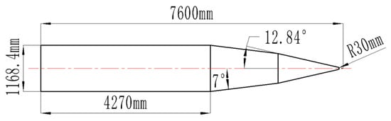
Figure 4.
Two-dimensional structure dimension drawing.
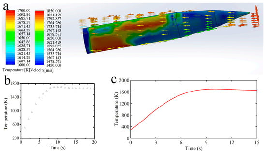
Figure 5.
Three-dimensional simulation drawing (a) of the hypersonic missile, sampling diagram (b) and curve fitting diagram (c) at the highest temperature of the hypersonic missile surface.
4.2. Comparative Simulations
Since the radiant heat element adopts a single spiral tungsten filament quartz lamp, the main parameters of GTESTD are listed: , , , , , , , , and .
In order to clearly verify the effectiveness of our proposed control strategy, the traditional PID control strategy, TDE-MFIPIDC strategy, global terminal sliding mode model-free intelligent PID control strategy based on the time delay observer (TDE-GTSMC-MFIPIDC) strategy are used as comparative simulations in Matlab/Simulink.
To ensure that the parameters of the proposed TDE-ANNGFOFTSMC-MFIPIDC strategy are appropriate, some simulation steps are applied.
Step 1: The period of simulation is 15 s, and the solver type is ode45 in Matlab/Simulation.
Step 2: Turn by increasing from negative to positive values until the control trend decreases when the other parameters satisfy the stability condition. The value of at the optimal control trend is selected.
Step 3: Turn from a large positive value to a small positive until the control trend declines, when other parameters are kept constant. The value of at the optimal control trend is selected.
Step 4: Turn , , , , and by satisfying , , and when other parameters are kept constant. The optimal value of each parameter is determined by observing the convergence speed and control accuracy.
Step 5: Turn , by satisfying and , when other parameters are kept constant. Determine the optimal parameters by tracking error and chattering.
Step 6: Finally, turn and when other parameters are kept constant. Determine the optimal parameters by tracking error and chattering.
To guarantee a fair comparison of the performance of each controller, the delay time of the control strategies based on TDE takes the same parameters. At the same time, a comparative analysis of the sign function and saturation function in the proposed control strategy. Some details of the compared control strategies are explained, and the specific parameters are listed in Table 2, Table 3 and Table 4.
Table 2.
The key parameters of the proposed TDE-ANNGFOFTSMC-MFIPIDC strategy.
Table 3.
The key parameters of the TDE-GTSMC-MFIPIDC strategy.
Table 4.
The key parameters of the TDE-MFIPIDC strategy and traditional PID control strategy.
Traditional PID control law:
TDE-MFIPIDC law:
where .
TDE-GTSMC-MFIPIDC strategy has a traditional GTSMS and an approach rate:
TDE-GTSMC-MFIPIDC law:
The simulation results are shown in Figure 6, Figure 7, Figure 8, Figure 9 and Figure 10, which include temperature response curves and tracking error curves for each control strategy.
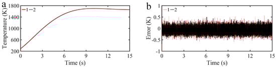
Figure 6.
Comparison results of temperature response curves (a) and tracking error curves (b) of the proposed control strategy under sign function and saturation function.
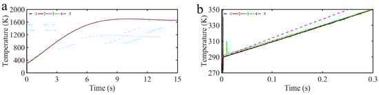
Figure 7.
Comparison results of temperature response curves (a) and partial enlarged curves (b) of TDE-ANNGFOFTSMC-MFIPIDC strategy (2), TDE-GTSMC-MFIPIDC strategy (3), TDE-MFIPIDC strategy (4) and traditional PID control strategy (5) to target temperature curve (1) without internal disturbances.
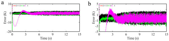
Figure 8.
Comparison results of tracking error curves (a) and partial enlarged curves (b) of TDE-ANNGFOFTSMC-MFIPIDC strategy (2), TDE-GTSMC-MFIPIDC strategy (3), TDE-MFIPIDC strategy (4) and traditional PID control strategy (5) to target temperature curve without internal disturbances.
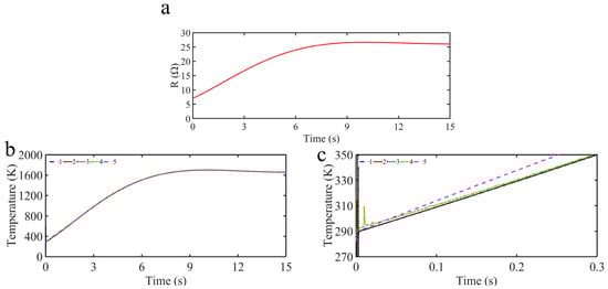
Figure 9.
Comparison results of temperature response curves (b) and partial enlarged curves (c), of TDE-ANNGFOFTSMC-MFIPIDC strategy (2), TDE-GTSMC-MFIPIDC strategy (3), TDE-MFIPIDC strategy (4) and traditional PID control strategy (5) to target temperature curve (1) with internal disturbances (a).
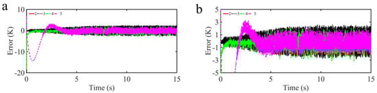
Figure 10.
Comparison results of tracking error curves (a) and partial enlarged curves (b) of TDE-ANNGFOFTSMC-MFIPIDC strategy (2), TDE-GTSMC-MFIPIDC strategy (3), TDE-MFIPIDC strategy (4) and traditional PID control strategy (5) to target temperature curves with internal disturbances.
Case : Comparison of sign function and saturation function in the proposed control strategy.
It can be seen that a sign function exists in our proposed controller, and the sign function may affect the chattering phenomenon. To verify whether the sign function influences the system, it is compared with the saturation function, which is as follows [32]:
where is the thickness of the boundary layer, is the design parameter.
The values of and , which are the same as in paper [32]. The simulation results are shown in Figure 6. From the error tracking curve, the saturation function is not significantly improved in control effect compared with the sign function [40,41,42,43]. Whether it is the saturation function or the sign function, both can lead to chattering issues in switched systems. In [44,45], Li highlighted that while MFC has traditionally been understood to operate on the premise of model-independent error dynamics, it actually serves as a model-based control technique to some extent, especially in power electronics. It demonstrates exceptional robustness against model variations compared to most existing model-based control methods. On the other hand, Park circumvented traditional modeling challenges by implementing a novel model-free voltage control strategy, effectively achieving superior voltage stability in smart grids during voltage recovery events. For switched systems with time-varying delays, MFC offers a distinctive advantage in mitigating the chattering phenomenon commonly observed in traditional switched control systems. By circumventing detailed system modeling, MFC ensures smoother control actions and reduces undesired high-frequency oscillations.
Case : Comparison of temperature response and tracking error without disturbances.
Figure 7a shows the temperature response results of our proposed control strategy, the TDE-GTSMC-MFIPIDC strategy, the TDE-MFIPIDC strategy and the traditional PID control strategy, and their partial enlarged curves are given in Figure 7b. Meanwhile, the tracking error curves and their partial enlarged curves for four control strategies are also given in Figure 8 to further demonstrate the control performance. As depicted in Figure 7a, effective target temperature curve tracking performance has been obtained with all four control strategies. According to the analysis of Figure 7b and Figure 8, we can see that the TDE-GTSMC-MFIPIDC strategy and the TDE-ANNGFOFTSMC-MFIPIDC strategy converge and stabilize almost at the initial moment, TDE-MFIPIDC strategy holds convergence at approximately 0.5 s, while the traditional PID control strategy holds convergence at approximately 4 s. Such a fast convergence speed is attributed to the fact that the TDE-MFIPIDC strategy, as the main controller, keeps convergence in a short time and the sliding mode control, as the auxiliary controller, further accelerates convergence in a short time. It can be seen from Figure 8 that the chattering amplitude of the TDE-GTSMC-MFIPIDC strategy, the TDE-MFIPIDC strategy and PID is more obvious at close to 2 K, while the chattering amplitude of the TDE-ANNGFOFTSMC-MFIPIDC strategy is only approximately 0.2 K, which is due to the role of FO and ANN in the designed sliding mode control strategy to ensure the control accuracy while suppressing the chattering phenomenon.
Therefore, our proposed TDE-ANNGFOFTSMC-MFIPIDC strategy is superior to the TDE-GTSMC-MFIPIDC strategy, the TDE-MFIPIDC strategy and the traditional PID control strategy in terms of response speed, convergence time, steady-state error, and chattering amplitude.
Case : Comparison of temperature response and tracking error with disturbances.
Considering the disturbances of test equipment in the real situation, the resistance of the quartz lamp heater will change with the increase in temperature, the increment of resistance is added to the Simulink simulation as internal disturbances. Figure 9a indicates the curve of internal disturbances versus temperature; the expression is as follows:
The simulation results are presented in Figure 9b,c and Figure 10. It is evident that all four simulated control strategies can provide effective control performance under time-varying disturbances. The proposed control strategy outperforms the comparison control strategies in terms of anti-interference ability. The internal disturbances have a greater impact on the TDE-GTSMC-MFIPIDC strategy, which is caused by the unknown upper bound of the estimation error and the selection of a large switching gain in order to maintain stability. However, the TDE-MFIPIDC strategy and the traditional PID control strategy ignore the effect of estimation error, and thus the effect of disturbances is not obvious. On the contrary, the TDE-MFIPIDC strategy does not consider the effect of estimation error, leading to reduced convergence speed and increased steady-state error.
For further quantitative comparison, the simulations calculation results for 0–15 s are shown in Table 5: the mean square error , the mean absolute error .
Table 5.
Simulations calculation results of MSE and MAE.
According to the results of the above four control strategy simulation figures and tables, the proposed control strategy performs better in terms of steady-state error, convergence speed and anti-interference ability.
5. Conclusions
This paper presents the design and analysis of a TDE-ANNGFOFTSMC-MFIPIDC approach for GTESTD temperature regulation. To circumvent the limitations of imprecise mathematical models, we employ an ultra-local model. Concurrently, TDE estimates and compensates for system disturbances and uncertainties. The IPID ensures convergence within a definite time frame. Recognizing the inherent estimation errors, a GFOFTSMC strategy acts as a supplementary controller, mitigating errors from TDE, accelerating convergence, ensuring finite-time response, and fortifying system robustness. Due to the indeterminacy of the upper bound of estimation errors, an ANN using the cubic B-spline function approximates the switching gain, thereby reducing chattering effects. System stability is validated using the Lyapunov and finite-time stability theorems. Cosimulation outcomes demonstrate the efficacy and robustness of the proposed control scheme for temperature tracking.
As we chart our path forward in this realm of research, our primary objective will be to delve deeper into devising methods that are both simpler and more efficient in addressing the chattering phenomenon, a persistent challenge in control systems. While our current approach predominantly hinges on adaptive switching gain, we believe that there might be other alternative solutions waiting to be explored. Notable among these are the saturation functions and the concept of approach rate. Both of these methods offer promising potential and could, in theory, streamline the control process even further. Beyond refining our methodologies, we are equally committed to practical validation. Recognizing the importance of real-world testing, we have slated plans to construct a test platform specifically tailored to simulate the aerodynamic, thermal environment. This is not just a mere expansion of our research infrastructure, but a step towards ensuring that our control algorithms are not merely theoretical marvels. Instead, by subjecting them to rigorous testing in a controlled environment that mimics real-world conditions, we aim to comprehensively demonstrate their reliability and effectiveness. This dual approach, combining innovative methodologies with empirical validation, will be our blueprint as we forge ahead in our quest for perfection.
Author Contributions
Conceptualization, X.L. and G.Z.; methodology, X.L.; software, M.Z. and Z.S.; validation, X.Z., M.Z. and Z.S.; formal analysis, X.L.; resources, G.Z.; data curation, Z.B.; writing—original draft preparation, Z.B.; writing—review and editing, X.L., G.Z, X.Z., Z.S. and M.Z.; visualization, X.Z.; supervision, Z.B.; project administration, G.Z.; funding acquisition, G.Z. All authors have read and agreed to the published version of the manuscript.
Funding
This research was supported by the Natural Science Foundation of Universities of Anhui Province (No. 2022AH051752, no. 2022AH051759).
Institutional Review Board Statement
Not applicable.
Informed Consent Statement
Not applicable.
Data Availability Statement
Data sharing not applicable.
Acknowledgments
The authors would like to express their gratitude to all those who helped them during the writing of this paper.
Conflicts of Interest
The authors declare no conflict of interest.
References
- Wang, F.; Fan, P.; Fan, Y.; Xu, B.; Yan, J. Robust adaptive control of hypersonic vehicle considering inlet unstart. J. Syst. Eng. Electron. 2022, 33, 188–196. [Google Scholar] [CrossRef]
- Niu, J.; Sui, Y.; Yu, Q.; Cao, X.; Yuan, Y.; Yang, X. Comparative numerical study of aerodynamic heating and performance of transonic hyperloop pods with different noses. Case Stud. Therm. Eng. 2022, 29, 101701. [Google Scholar] [CrossRef]
- Zhang, Z.; Hao, C.; Fang, R.; Wu, Z.; Li, H.; Kong, F. Modal Characteristics of Carbon Fiber Reinforced Composite Structure at High Temperature. J. Spacecr. Rocket. 2021, 58, 182–189. [Google Scholar] [CrossRef]
- Cheng, L.; Wang, Z.; Gong, S. Adaptive control of hypersonic vehicles with unknown dynamics based on dual network architecture. Acta Astronaut. 2022, 193, 197–208. [Google Scholar] [CrossRef]
- Dalboni, M.; Tavernini, D.; Montanaro, U.; Soldati, A.; Concari, C.; Dhaens, M.; Sorniotti, A. Nonlinear Model Predictive Control for Integrated Energy-Efficient Torque-Vectoring and Anti-Roll Moment Distribution. Ieee Asme Trans. Mechatron. 2021, 26, 1212–1224. [Google Scholar] [CrossRef]
- Favato, A.; Carlet, P.G.; Toso, F.; Torchio, R.; Bolognani, S. Integral Model Predictive Current Control for Synchronous Motor Drives. Ieee Trans. Power Electron. 2021, 36, 13293–13303. [Google Scholar] [CrossRef]
- Mofid, O.; Mobayen, S. Adaptive sliding mode control for finite-time stability of quad-rotor UAVs with parametric uncertainties. Isa Trans. 2018, 72, 1–14. [Google Scholar] [CrossRef] [PubMed]
- Fliess, M.; Join, C. Model-free control. Int. J. Control 2013, 86, 2228–2252. [Google Scholar] [CrossRef]
- Fliess, M.; Join, C. An alternative to proportional-integral and proportional-integral-derivative regulators: Intelligent proportional-derivative regulators. Int. J. Robust Nonlinear Control. 2022, 32, 9512–9524. [Google Scholar] [CrossRef]
- Chand, A.N.; Kawanishi, M.; Narikiyo, T. Non-linear model-free control of flapping wing flying robot using iPID. In Proceedings of the 2016 IEEE International Conference on Robotics and Automation (ICRA), Stockholm, Sweden, 16–21 May 2016. [Google Scholar]
- Saleki, A.; Fateh, M.M. Model-free control of electrically driven robot manipulators using an extended state observer. Comput. Electr. Eng. 2020, 87, 106768. [Google Scholar] [CrossRef]
- Liu, J.; Li, X.; Li, J.; Wang, K.; Wang, F.; Cui, G. Model-Free Adaptive Control of pH Value of Wet Desulfurization Slurry under Switching of Multiple Working Conditions. Complexity 2020, 2020, 4727412. [Google Scholar] [CrossRef]
- Tran, M.-T.; Lee, D.-H.; Chakir, S.; Kim, Y.-B. A Novel Adaptive Super-Twisting Sliding Mode Control Scheme with Time-Delay Estimation for a Single Ducted-Fan Unmanned Aerial Vehicle. Actuators 2021, 10, 54. [Google Scholar] [CrossRef]
- Wang, X.; Zhang, R.; Li, G.; Wang, Q.; Wen, Y. Time Delay Estimation Control of Permanent Magnet Spherical Actuator Based on Gradient Compensation. Electronics 2022, 11, 66. [Google Scholar] [CrossRef]
- Han, S.; Wang, H.; Tian, Y.; Christov, N. Time-delay estimation based computed torque control with robust adaptive RBF neural network compensator for a rehabilitation exoskeleton. ISA Trans. 2020, 97, 171–181. [Google Scholar] [CrossRef]
- Kali, Y.; Rodas, J.; Gregor, R.; Saad, M.; Benjelloun, K. Attitude tracking of a tri-rotor UAV based on robust sliding mode with time delay estimation. In Proceedings of the 2018 International Conference on Unmanned Aircraft Systems (ICUAS), Dallas, TX, USA, 12–15 June 2018; pp. 346–351. [Google Scholar]
- Li, Z.; Wang, P.; Zhang, J.; Guan, H. A model-free method for identifying time-delay characteristics of HVAC system based on multivariate transfer entropy. Build. Environ. 2022, 217, 109072. [Google Scholar] [CrossRef]
- Zhang, X.; Liu, J. Model-free Attitude Decoupling Control of Space Robots Based on Time-delay Estimation. J. Astronaut. 2021, 42, 1150–1161. [Google Scholar]
- Pukdeboon, C. Output Feedback Second Order Sliding Mode Control for Spacecraft Attitude and Translation Motion. Int. J. Control Autom. Syst. 2016, 14, 411–424. [Google Scholar] [CrossRef]
- Yang, Y.; Yan, Y.; Xu, X. Fractional Order Adaptive Fast Super-Twisting Sliding Mode Control for Steer-by-Wire Vehicles with Time-Delay Estimation. Electronics 2021, 10, 2424. [Google Scholar] [CrossRef]
- Wang, J.; Bi, C.; Wang, D.; Kuang, Q.; Wang, C. Finite-time distributed event-triggered formation control for quadrotor UAVs with experimentation. ISA Trans. 2022, 126, 585–596. [Google Scholar] [CrossRef]
- Ren, Y.; Wang, H.; Xie, D.; Yue, M.; Weng, K.; Gao, W.; Liu, N. New Terminal Sliding Mode Consensus Algorithm for Disturbed Second-order Multi-agent Systems. Int. J. Control Autom. Syst. 2022, 20, 2534–2542. [Google Scholar] [CrossRef]
- Tong, X.; Zhao, H.; Feng, G. Adaptive global terminal sliding mode control for anti-warship missiles. In Proceedings of the 2006 6th World Congress on Intelligent Control and Automation, Dalian, China, 21–23 June 2006; pp. 1962–1966. [Google Scholar]
- Cao, P.; Fan, H.; Cai, Z. Adaptive fractional-order PID control for VSC-HVDC systems via cooperative beetle antennae search with offshore wind integration. Energy Eng. 2021, 118, 265–284. [Google Scholar] [CrossRef]
- Roy, P.; Roy, B.K. Sliding mode control versus fractional-order sliding mode control: Applied to a magnetic levitation system. J. Control Autom. Electr. Syst. 2020, 31, 597–606. [Google Scholar] [CrossRef]
- Xiong, T.; Pu, Z.; Yi, J.; Tao, X. Fixed-time observer based adaptive neural network time-varying formation tracking control for multi-agent systems via minimal learning parameter approach. IET Control. Theory Appl. 2020, 14, 1147–1157. [Google Scholar] [CrossRef]
- Li, Y.; Sai, H.; Zhu, M.; Xu, Z.; Mu, D. Neural network-based continuous finite-time tracking control for uncertain robotic systems with actuator saturation. Asian J. Control 2022, 24, 3475–3493. [Google Scholar] [CrossRef]
- Lv, X.; Zhang, G.; Zhu, M.; Shi, Z.; Bai, Z.; Alexandrov, I.V. Aerodynamic Heating Ground Simulation of Hypersonic Vehicles Based on Model-Free Control Using Super Twisting Nonlinear Fractional Order Sliding Mode. Mathematics 2022, 10, 1664. [Google Scholar] [CrossRef]
- Xia, L.S.; Bin, Q.I.; Tian, N.; Cao, Y.Q.; Hong-Liang, L.I. Study on Modeling Analysis and Testing Method of Electro-thermal Properties of Quartz Lamp. Infrared Technol. 2015, 37, 877. (In Chinese) [Google Scholar]
- Lv, X.; Zhang, G.; Zhu, M.; Ouyang, H.; Shi, Z.; Bai, Z.; Alexandrov, I.V. Adaptive Neural Network Global Nonsingular Fast Terminal Sliding Mode Control for a Real Time Ground Simulation of Aerodynamic Heating Produced by Hypersonic Vehicles. Energies 2022, 15, 3284. [Google Scholar] [CrossRef]
- Gao, P.; Zhang, G.M.; Ouyang, H.M.; Mei, L. An Adaptive Super Twisting Nonlinear Fractional Order PID Sliding Mode Control of Permanent Magnet Synchronous Motor Speed Regulation System Based on Extended State Observer. Ieee Access 2020, 8, 53498–53510. [Google Scholar] [CrossRef]
- Wu, G.Q.; Wu, S.N.; Wu, Z.G. Robust Finite-Time Control for Spacecraft with Coupled Translation and Attitude Dynamics. Math. Probl. Eng. 2013, 2013, 7070485. [Google Scholar] [CrossRef]
- Wang, Y.; Gu, L.; Gao, M.; Zhu, K. Multivariable Output Feedback Adaptive Terminal Sliding Mode Control for Underwater Vehicles. Asian J. Control 2016, 18, 247–265. [Google Scholar] [CrossRef]
- Ahmed, S.; Wang, H.P.; Tian, Y. Model-free control using time delay estimation and fractional-order nonsingular fast terminal sliding mode for uncertain lower-limb exoskeleton. J. Vib. Control 2018, 24, 5273–5290. [Google Scholar] [CrossRef]
- Wang, Y.Y.; Chen, J.W.; Yan, F.; Zhu, K.W.; Chen, B. Adaptive super-twisting fractional-order nonsingular terminal sliding mode control of cable-driven manipulators. Isa Trans. 2019, 86, 163–180. [Google Scholar] [CrossRef]
- Li, S.Z.; Wang, H.P.; Tian, Y.; Aitouch, A.; Klein, J. Direct power control of DFIG wind turbine systems based on an intelligent proportional-integral sliding mode control. Isa Trans. 2016, 64, 431–439. [Google Scholar] [CrossRef]
- Zhang, X.Y.; Wang, H.P.; Tian, Y.; Peyrodie, L.; Wang, X.K. Model-free based neural network control with time-delay estimation for lower extremity exoskeleton. Neurocomputing 2018, 272, 178–188. [Google Scholar] [CrossRef]
- Wang, H.P.; Ye, X.F.; Tian, Y.; Zheng, G.; Christov, N. Model-Free-Based Terminal SMC of Quadrotor Attitude and Position. IEEE Trans. Aerosp. Electron. Syst. 2016, 52, 2519–2528. [Google Scholar] [CrossRef]
- Chen, Y.J.; Liang, J.C.; Wu, Y.N.; Miao, Z.Q.; Zhang, H.; Wang, Y.N. Adaptive Sliding-Mode Disturbance Observer-Based Finite-Time Control for Unmanned Aerial Manipulator With Prescribed Performance. IEEE T. Cybern. 2023, 53, 3263–3276. [Google Scholar] [CrossRef]
- He, H.; Gao, X.; Qi, W. Asynchronous H-infinity control of time-delayed switched systems with actuator saturation via anti-windup design. Optim. Control Appl. Methods 2018, 39, 1–18. [Google Scholar] [CrossRef]
- Event-triggered Control of Positive Switched Systems with Actuator Saturation and Time-delay. Int. J. Autom. Comput. 2021, 18, 141–154. [CrossRef]
- Sobhanipour, H.; Rezaie, B. Enhanced Exponential Stability Analysis for Switched Linear Time-Varying Delay Systems Under Admissible Edge-Dependent Average Dwell-Time Strategy. Ieee Trans. Syst. Man Cybern. Syst. 2023, 53, 5331–5342. [Google Scholar] [CrossRef]
- Wang, P.; Sang, H.; Ma, D. Dissipativity for Discrete-Time Switched Positive Delay Systems: A Dwell-Time-Dependent Linear Copositive Storage Functional Method. Ieee Trans. Syst. Man Cybern. Syst. 2023, 53, 4028–4038. [Google Scholar] [CrossRef]
- Park, B.; Olama, M.M. A Model-Free Voltage Control Approach to Mitigate Motor Stalling and FIDVR for Smart Grids. Ieee Trans. Smart Grid 2021, 12, 67–78. [Google Scholar] [CrossRef]
- Li, W.; Yuan, H.; Li, S.; Zhu, J. A Revisit to Model-Free Control. Ieee Trans. Power Electron. 2022, 37, 14408–14421. [Google Scholar] [CrossRef]
Disclaimer/Publisher’s Note: The statements, opinions and data contained in all publications are solely those of the individual author(s) and contributor(s) and not of MDPI and/or the editor(s). MDPI and/or the editor(s) disclaim responsibility for any injury to people or property resulting from any ideas, methods, instructions or products referred to in the content. |
© 2023 by the authors. Licensee MDPI, Basel, Switzerland. This article is an open access article distributed under the terms and conditions of the Creative Commons Attribution (CC BY) license (https://creativecommons.org/licenses/by/4.0/).