On the Size of the Safety Area around the Launch Trajectory of a Rocket

Abstract

The safety zone around the flight path of a rocket is determined by the fall of debris in the case of an accidental explosion or commanded termination. The trajectory of a tumbling body in a vertical plane is determined by specifying the velocity, flight path angle and angle of attack as functions of time. This involves the lift, drag and pitching moment coefficients as functions of the angle of attack over a full circle—0 to 360 degrees—to account for the tumbling motion. The problem is reduced to a third-order non-linear differential equation for the angle of attack by using the approximation of free fall coordinates. The analytical and numerical solutions show that two types of tumbling fall are possible, one with rotation and the other with oscillation. The tumbling trajectories are plotted and discussed for a variety of initial conditions, mass and aerodynamic properties of the tumbling body.

1. Introduction

The launch of rockets into space is surrounded by strict safety precautions such as the exclusion of flying over populated areas. More specifically, when a rocket is launched, there is a safety zone on the ground below and around its flight path in case of a propulsion loss, or an explosion or intentional self-destruct instruction following a failure. The safety zone must be large enough so that any potential debris falls within it. Nowadays, in the space industry, the concept of range safety—application of safety policies, principles and techniques to protect the public, workforce and/or property from hazards associated with range operations [1]—is of the utmost importance.

Range safety is assured through the inclusion of a flight termination system (FTS) aboard the spacecraft. The FTSs are highly reliable systems with extensive emphasis on redundancy and pre-launch testing [2], which are capable of terminating powered flight upon command, for instance by shutting down the main propulsion system of the rocket [3], leaving the debris to fall into an abandoned area. The FTS is activated based on the deviations of flight attitude and range safety criteria, i.e., if the rocket strays away from its intended path leaving its previously assigned safety zone [4].

The uncertainties about the trajectory of tumbling debris lead to a safety area that is possibly larger than it needed to be. For launch sites having nearby population centres, a large safety area may severely limit the range of allowable azimuths and require the use of non-optimal flight paths. The method of calculation of the trajectory of a tumbling body applies to the following: (i) the debris resulting from an accidental explosion or commanded flight termination; (ii) a spent stage of a rocket after burn-out; (iii) the whole rocket or a single stage after burn-out or propulsion failure at an earlier stage of flight.

The trajectory of a tumbling body is calculated in a vertical plane (Section 2) and the tumbling motion requires the specification of the aerodynamic coefficients over the full circle (zero to 360 degrees) of angles of attack (Section 3). With some simplifying assumptions, it is shown that the angle of attack satisfies a non-linear third-order differential equation (Section 3) whose unique solution involves three independent initial conditions. Both analytic solutions (Section 4) and numeric solutions (Section 5) show the existence of two regimes of fall, one with rotation and the other with oscillation. These two regimes are demonstrated over a wide range of initial conditions (Section 6) and rocket parameters (Section 7) of the tumbling body. Some observations about the results obtained in the previous sections and the conclusions are presented in the last part (Section 8).

2. Flight in a Vertical Plane

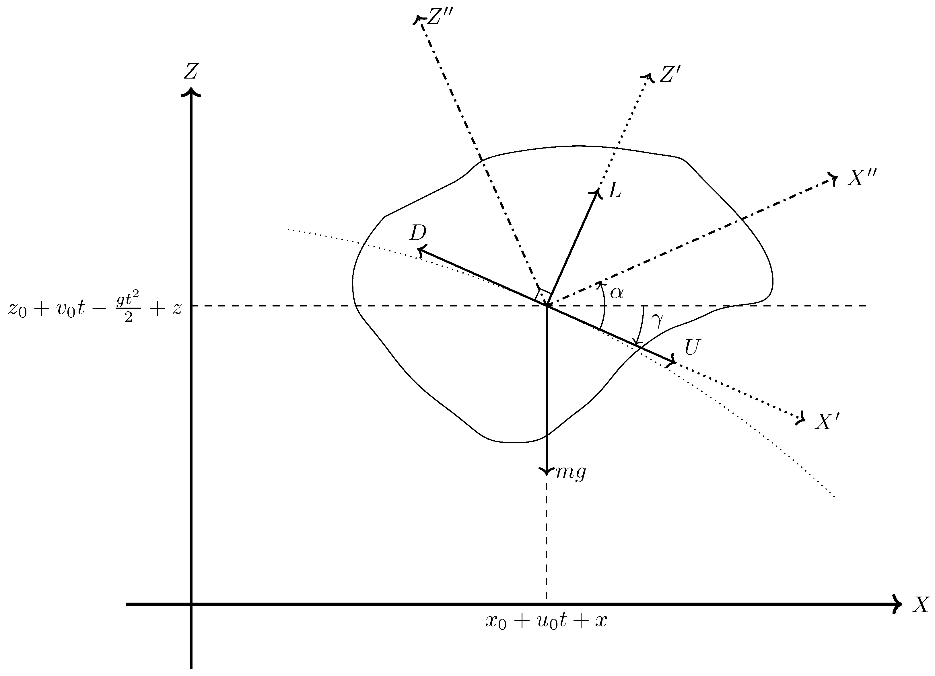
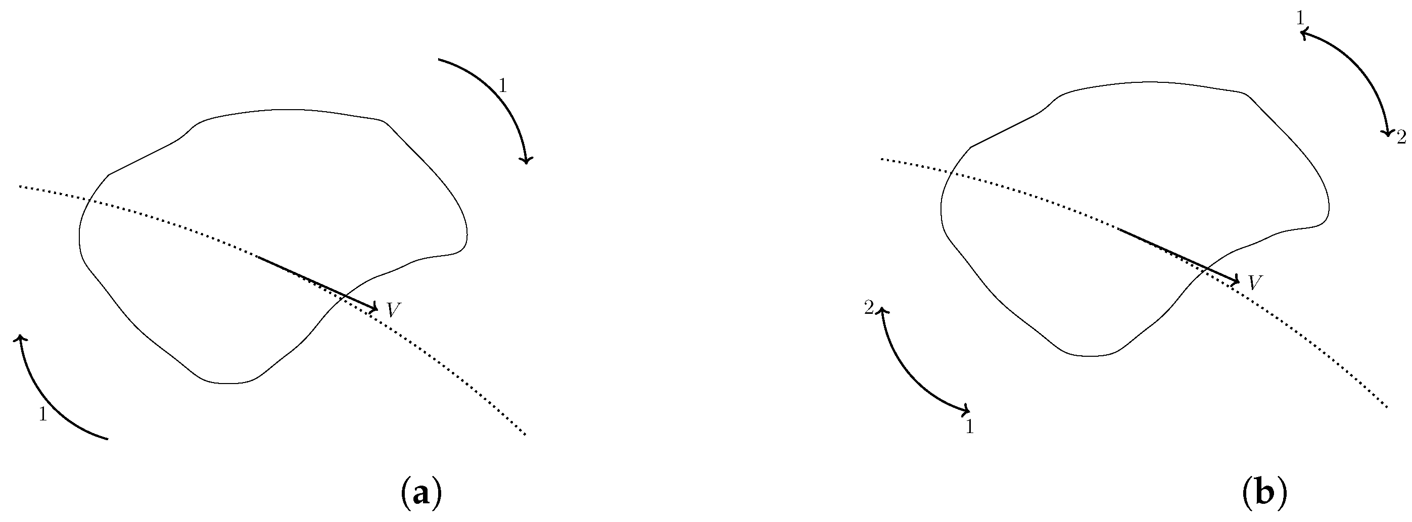
The tumbling motion of the body is considered in a vertical plane, and three sets of orthogonal axes are shown in Figure 1: (i) Earth fixed axis, with altitude Z and opposite gravity g, and coordinate X along flat ground; (ii) wind axis, with $X^{\prime }$ along airspeed U and opposite to drag, and $Z^{\prime }$ orthogonal along the lift L; (iii) body axis with $X^{″}$ along the aircraft datum and $Z^{″}$ orthogonal. The angle between $X^{″}$ and $X^{\prime }$ is the angle of attack $\alpha$, and the angle between $X^{\prime }$ and X is the flight path angle $\gamma$. Equations of motion in a vertical plane are written in wind axis, so that the wind velocity is included in the airspeed V, and they state the balance of forces tangent—Equation (1a)—and normal—Equation (1b)—to the flight path and the pitching moment—Equation (1c):

$$\begin{array}{cc}\hfill m\frac{\mathrm{d}U}{\mathrm{d}t}& =-D-mgsin\left(\gamma \right),\hfill \end{array}$$

(1a)

$$\begin{array}{cc}\hfill mU\frac{\mathrm{d}\gamma }{\mathrm{d}t}& =L-mgcos\left(\gamma \right),\hfill \end{array}$$

(1b)

$$\begin{array}{cc}\hfill I\left(\frac{{\mathrm{d}}^2\alpha }{\mathrm{d}{t}^2}-\frac{{\mathrm{d}}^2\gamma }{\mathrm{d}{t}^2}\right)& =M,\hfill \end{array}$$

(1c)

where U is the modulus of the total velocity, $\gamma$ is the total flight path angle, L is the lift, D is the drag, m is the mass, I is the pitch moment of inertia, $\alpha$ is the angle of attack, $\alpha -\gamma$ is the pitch angle, M is the pitching moment and g is the acceleration of gravity. Since the motion of the tumbling body is unpowered, there is no thrust in the previous equations.

The Cartesian coordinates of the trajectory, $X\left(t\right)$ and $Z\left(t\right)$, in a vertical plane are decomposed into the sum of the following: (i) a parabolic free fall under uniform gravity; (ii) a perturbation, $x\left(t\right)$ and $z\left(t\right)$, due to the aerodynamic forces:

$$\begin{array}{cc}\hfill X\left(t\right)& =x_0+u_{0}t+x\left(t\right),\hfill \end{array}$$

(2a)

$$\begin{array}{cc}\hfill Z\left(t\right)& =z_0+v_{0}t-\frac{1}{2}g{t}^2+z\left(t\right).\hfill \end{array}$$

(2b)

In Equations (2a) and (2b), the pair $\left(x_0,z_0\right)$ corresponds to the initial position of the body and the pair $\left(u_0,v_0\right)$ is associated to the initial velocity components due to the gravitational force; however, it will be assumed that the last pair is $\left(0,0\right)$ and consequently the components of the total initial velocity are given by the pair $\left[\dot{x}\left(0\right),\dot{z}\left(0\right)\right]$.

The horizontal and vertical velocities are obtained by differentiating, respectively, Equations (2a) and (2b):

$$\begin{array}{cc}\hfill \dot{X}\left(t\right)& =\frac{\mathrm{d}}{\mathrm{d}t}\left[x_0+u_{0}t+x\left(t\right)\right]=u_0+\dot{x}\left(t\right),\hfill \end{array}$$

(3a)

$$\begin{array}{cc}\hfill \dot{Z}\left(t\right)& =\frac{\mathrm{d}}{\mathrm{d}t}\left[z_0+v_{0}t-\frac{1}{2}g{t}^2+z\left(t\right)\right]=v_0-gt+\dot{z}\left(t\right),\hfill \end{array}$$

(3b)

that imply Equation (4b) for the modulus of the total velocity (4a):

$$\begin{array}{}\mathrm{(4a)}& {\left[U\left(t\right)\right]}^2\equiv {\left[\dot{X}\left(t\right)\right]}^2+{\left[\dot{Z}\left(t\right)\right]}^2\mathrm{(4b)}& \hspace{1em}\hspace{1em}\hspace{1em}\hspace{1em}\hspace{1em}={\left[u_0+\dot{x}\left(t\right)\right]}^2+{\left[v_0-gt+\dot{z}\left(t\right)\right]}^2,\end{array}$$

and is related to the modulus of the relative velocity V in free fall coordinates by

$$\begin{array}{}\mathrm{(4c)}& {\left[V\left(t\right)\right]}^2\equiv {\left[\dot{x}\left(t\right)\right]}^2+{\left[\dot{z}\left(t\right)\right]}^2\mathrm{(4d)}& \hspace{1em}\hspace{1em}\hspace{1em}\hspace{1em}\hspace{1em}\hspace{1em}\hspace{1em}={\left[U\left(t\right)\right]}^2-2u_0\dot{X}\left(t\right)-2\left(v_0-gt\right)\dot{Z}\left(t\right)+{\left(u_0\right)}^2+{\left(v_0-gt\right)}^2.\end{array}$$

The components of the total velocity in Earth fixed coordinates

$$\begin{array}{cc}\hfill \dot{X}& =Ucos\gamma ,\hfill \end{array}$$

(5a)

$$\begin{array}{cc}\hfill \dot{Z}& =Usin\gamma ,\hfill \end{array}$$

(5b)

agree with the total flight path angle:

$$\frac{\dot{Z}}{\dot{X}}=tan\gamma ,$$

(5c)

and the components of the relative velocity (3a) and (3b) in free fall coordinates

$$\begin{array}{cc}\hfill \dot{x}& =Ucos\gamma -u_0,\hfill \end{array}$$

(6a)

$$\begin{array}{cc}\hfill \dot{z}& =Usin\gamma -v_0+gt,\hfill \end{array}$$

(6b)

lead to the relative flight path angle:

$$tan\delta \equiv \frac{\dot{z}}{\dot{x}}=\frac{Usin\gamma -v_0+gt}{Ucos\gamma -u_0}.$$

(6c)

Substituting (5a) and (5b) in (4d) leads to the following:

$$0=U^2-\left[2u_{0}cos\gamma +2\left(v_0-gt\right)sin\gamma \right]U+{\left(u_0\right)}^2+{\left(v_0-gt\right)}^2-V^2,$$

(7a)

whose roots specify the total velocity in Earth fixed reference frame U in terms of the relative velocity V in free fall coordinates

$$U=u_{0}cos\gamma +\left(v_0-gt\right)sin\gamma \pm {\left|V^2-{\left[u_{0}sin\gamma -\left(v_0-gt\right)cos\gamma \right]}^2\right|}^{1/2}.$$

(7b)

Here, the flight path angle $\gamma$ and initial velocities $\left(u_0,v_0\right)$, along with acceleration due to gravity g and time t, explicitly and implicitly appear in $\left(V,\gamma \right)$.

The three coupled equations of motion—Equations (1a) to (1c)—form a fourth-order system. Since free fall coordinates (2a) and (2b) already include gravity, the approximation is made that, in the free fall reference frame, gravity can be omitted from Equations of motion. This free fall coordinate approximation will be checked in subsequent work, considering the same problem without this approximation. As a simpler preliminary approach to the problem, the free fall coordinate approximation is made, leading to a third-order system, as shown below. Thus, the free fall coordinate approximation includes the effect of gravity in the moving non-Galilean reference frame (2a) and (2b), but omits it in Equations of motion:

$$\begin{array}{c}\hfill m\frac{\mathrm{d}V}{\mathrm{d}t}=-\frac{1}{2}\rho S{V}^2{C}_D\left(\alpha \right),\end{array}$$

(8a)

$$\begin{array}{c}\hfill mV\frac{\mathrm{d}\delta }{\mathrm{d}t}=\frac{1}{2}\rho S{V}^2{C}_L\left(\alpha \right),\end{array}$$

(8b)

$$\begin{array}{c}\hfill I\left(\frac{{\mathrm{d}}^2\alpha }{\mathrm{d}{t}^2}-\frac{{\mathrm{d}}^2\gamma }{\mathrm{d}{t}^2}\right)=\frac{1}{2}\rho Sl{V}^2{C}_M\left(\alpha \right),\end{array}$$

(8c)

where $C_L$, $C_D$ and $C_M$ are respectively the lift, drag and pitching moment coefficients that are assumed to depend only on the angle of attack, l is a reference length and V is the velocity in free fall coordinates. The free fall coordinate approximation retains the angles of attack $\alpha$ and flight path angle $\gamma$, with the supposition that the absolute and relative flight path angles are of the same order $\gamma \sim \delta$, and assumes that the acceleration of the latter is much smaller than that of the angle of attack $\ddot{\gamma }\ll \ddot{\alpha }$, so that Equations (8a) to (8c) after simplification of (8c) become

$$\begin{array}{c}\hfill m\frac{\mathrm{d}V}{\mathrm{d}t}=-\frac{1}{2}\rho S{V}^2{C}_D\left(\alpha \right),\end{array}$$

(9a)

$$\begin{array}{c}\hfill mV\frac{\mathrm{d}\delta }{\mathrm{d}t}=\frac{1}{2}\rho S{V}^2{C}_L\left(\alpha \right),\end{array}$$

(9b)

$$\begin{array}{c}\hfill I\frac{{\mathrm{d}}^2\alpha }{\mathrm{d}{t}^2}=\frac{1}{2}\rho Sl{V}^2{C}_M\left(\alpha \right),\end{array}$$

(9c)

Consequently the relative velocity is expressed in terms of the angle of attack by solving Equation (9c) as follows:

$$V=\sqrt{\frac{2I\ddot{\alpha }}{\rho Sl{C}_M\left(\alpha \right)}}.$$

(10)

Substitution of Equation (10) into Equation (9a) leads to a differential equation for the angle of attack alone:

$$\frac{\mathrm{d}}{\mathrm{d}t}\left[\sqrt{\frac{2I\ddot{\alpha }}{\rho Sl{C}_M\left(\alpha \right)}}\right]=-\frac{\rho S}{2m}{C}_D\left(\alpha \right)\frac{2I\ddot{\alpha }}{\rho Sl{C}_M\left(\alpha \right)},$$

(11a)

that is of the third-order and can be rewritten with an explicit third-order derivative:

$$\begin{array}{c}\hfill \stackrel{⃛}{\alpha }-\ddot{\alpha }\frac{{\dot{C}}_M}{C_M}=-\frac{I}{ml}\frac{C_D}{C_M}\sqrt{\frac{2\rho Sl}{I}}\sqrt{\frac{\ddot{\alpha }}{C_M}}{C}_M\ddot{\alpha }=-\sqrt{\frac{I}{m}}\sqrt{\frac{\rho Sl}{m}}\frac{C_D}{l}\sqrt{\frac{2}{C_M}}{\ddot{\alpha }}^{3/2}.\end{array}$$

(11b)

In the last equation appear the following: (i) the radius of gyration r that is related to the moment of inertia I and mass m by the relation:

$$I=m{r}^2;$$

(12a)

(ii) the dimensionless mass factor defined by the fraction

$$\mu \equiv \frac{\rho Sl}{m}<1,$$

(12b)

as the ratio of the mass of a cylinder of air with density $\rho$, cross-section S and length l to the mass m of the tumbling body. The mass factor is less than unity if the tumbling body is heavier than its volume of air that it displaces; this should be nearly always the case by some margin. Using Equations (12a) and (12b) in Equation (11b), the third order differential equation becomes

$$\stackrel{⃛}{\alpha }-\ddot{\alpha }\frac{{\dot{C}}_M}{C_M}=-\frac{r}{l}\sqrt{\frac{2\mu }{C_M}}{C}_D{\ddot{\alpha }}^{3/2}.$$

(13)

This equation is nonlinear and remains valid for any form of drag coefficient $C_D$ and pitching moment coefficient $C_M$, both of which depend solely on the angle of attack. The solution of Equation (13) specifies the angle of attack as a function of time $\alpha \left(t\right)$ and substitution in Equation (10) specifies the modulus of the relative velocity $V\left(t\right)$. The substitution of Equation (10) in Equation (9b) leads to the following:

$$\dot{\delta }=\frac{\rho S}{2m}{C}_L\left(\alpha \right)\sqrt{\frac{2I\ddot{\alpha }}{\rho Sl{C}_M}}=\frac{r}{l}{C}_L\sqrt{\frac{\mu }{2C_M}}{\ddot{\alpha }}^{1/2}.$$

(14)

This equation specifies by integration the relative flight path angle $\delta \left(t\right)$. The initial conditions for the third-order differential equation are the angle of attack and its first- and second-order time derivatives; the formula for the modulus of the relative velocity V (10), arranged in the way:

$$\ddot{\alpha }=\frac{\rho Sl}{2I}{V}^2{C}_M\left(\alpha \right)=\frac{\mu }{2}{\left(\frac{V}{r}\right)}^2{C}_M\left(\alpha \right),$$

(15)

is used to evaluate the second-order time derivative of the angle of attack $\ddot{\alpha }$, particularly at initial time.

So far, no assumptions have been made on the dependence of the drag, lift and pitching moment coefficients on the angle of attack.

3. Aerodynamic Coefficients in a Full Circle

In order to consider tumbling motion, the aerodynamic coefficients must be specified for the full range of angles of attack. Although the behaviours of lift, drag and pitching moment coefficients have been thoroughly studied for small angles of attack for aerofoils or streamlined shapes, this is not the case for the tumbling motion of irregular shaped bodies, considering the full revolution of angles of attack. In order to extend the “usual” aerodynamic theory to tumbling motion, some simple plausible assumptions are made.

For the lift coefficient, the starting point is the expression for the lift coefficient for aerofoils at small angles of attack [5,6], where $C_{L_{\alpha }}$ corresponds to the slope for small angles of attack and the angle is measured relative to zero lift:

$$C_L\left(\alpha \right)=C_{L_{\alpha }}sin\left(\alpha \right).$$

(16)

For a tumbling body, the lift coefficient should obey three conditions: (i) for small angles of attack, the resulting expression should be the same (16) as the one obtained using small angle theory; (ii) when the body is perpendicular to the flow ($\alpha =\pi /2$) there should be no lift; (iii) the lift coefficient variation must be periodic with period $\pi$. Equation (16) does not meet the third requirement. Multiplying Equation (16) by $cos\alpha$ leads to the following:

$$C_L\left(\alpha \right)=C_{L_{\alpha }}sin\left(\alpha \right)cos\left(\alpha \right)=\frac{1}{2}{C}_{L_{\alpha }}sin\left(2\alpha \right).$$

(17)

This equation meets all three requirements: (i) for small angle of attack, ${\alpha }^2<<1$ then $cos\alpha \sim 1$ and the expression (17) reduces to (16); (ii) if the body is perpendicular to the flow, $\alpha =\pi /2$ then $cos\alpha =0$ and the lift coefficient (17) is zero; (iii) the lift coefficient (17) is a periodic function with period $\pi$, since $sin\left[2\left(\alpha +\pi \right)\right]=sin\left(2\alpha \right)$.

The next aerodynamic coefficient to be considered is the pitching moment coefficient. Since the pitching moment is taken relative to the centre of mass of the rocket whereas the lift is applied in the centre of pressure, the pitching moment can be assumed to be proportional to the lift:

$$M=aL,$$

(18)

through the distance a between the centre of pressure and the centre of mass of the rocket. The dependence of the pitching moment on the angle of attack is thus similar to Equation (17), with a distinct pitching moment slope in the next equation:

$$C_M\left(\alpha \right)=\frac{1}{2}{C}_{M_{\alpha }}sin\left(2\alpha \right),$$

(19)

in which the derivative of the coefficient moment is proportional to the derivative of the lift coefficient with respect to the angle of attack through the following relation:

$$C_{M_{\alpha }}\equiv \frac{a}{l}{C}_{L_{\alpha }},$$

(20)

that follows from

$$a=\frac{M}{L}=\frac{l{C}_M\left(\alpha \right)}{C_L\left(\alpha \right)}=l\frac{C_{M_{\alpha }}}{C_{L_{\alpha }}}.$$

(21)

The relation (17) also implies

$${\dot{C}}_M\left(\alpha \right)\equiv \frac{\mathrm{d}{C}_M}{\mathrm{d}t}=\frac{\mathrm{d}\alpha }{\mathrm{d}t}\frac{\mathrm{d}{C}_M}{\mathrm{d}\alpha }=\dot{\alpha }{C}_{M_{\alpha }}cos\left(2\alpha \right).$$

(22)

The only aerodynamic coefficient still to be considered is the drag coefficient. The drag coefficient will be given by the sum of three terms, of which the first two are the usual in aerodynamic theory [7]:

$$C_D\left(\alpha \right)=C_{D_0}+K{\left[C_L\left(\alpha \right)\right]}^2+\frac{2\pi sin\left(\alpha \right)}{4+\pi sin\left(\alpha \right)},$$

(23)

namely: (i) the first term, specifically $C_{D_0}$, is independent from the angle of attack and represents the friction drag; (ii) the second term is proportionate to the square of the lift coefficient, which ensures a parabolic lift–drag relationship and is commonly referred to as induced drag. To accommodate the wide angle of attack experienced by a tumbling body, a third term is introduced, representing the "wake drag" of a lamina at an angle $\alpha$ relative to a stream that features a "vacuous" region behind it. This region lies between the free streamlines originating from the lamina’s tips [5,6].

The expressions for the pitching moment coefficient (19) and its time derivative (22) appear in the non-linear third-order differential Equation (11b) for the angle of attack, whose square takes the following form:

$${\left[\stackrel{⃛}{\alpha }-2\ddot{\alpha }\dot{\alpha }\frac{cos\left(2\alpha \right)}{sin\left(2\alpha \right)}\right]}^2=\frac{4}{C_{M_{\alpha }}}\frac{I}{m{l}^2}\frac{\rho Sl}{m}\frac{{\ddot{\alpha }}^3}{sin\left(2\alpha \right)}{\left[C_D\left(\alpha \right)\right]}^2,$$

(24)

whose right-hand side involves: (i) the drag and pitching moment coefficients that depend on angle of attack; (ii) two dimensionless parameters that do not depend on any of aerodynamic coefficients. The first dimensionless parameter ${ϵ}_0$ is the moment of inertia of the rocket divided by the product of the mass by the square of the lengthscale:

$${ϵ}_0\equiv \frac{I}{m{l}^2}={\left(\frac{r}{l}\right)}^2<1.$$

(25)

The lengthscale can be taken to be the rocket length, which is usually greater than the radius of gyration relative to the pitch axis, so that ${ϵ}_0$ is less than unity. The second dimensionless parameter $ϵ$ equals the first parameter (25) multiplied by the mass ratio (12b), which is also smaller than unity:

$$ϵ\equiv {ϵ}_0\mu =\frac{r^2}{l^2}\frac{\rho Sl}{m}=\frac{\rho S{r}^2}{ml}=\frac{\rho SI}{m^{2}l}<1,$$

(26)

so that their product is also less than unity. Using the parameter $ϵ$ obtained in Equation (26), the non-linear third order differential equation for the angle of attack (24) becomes

$$\begin{array}{c}\hfill \frac{4ϵ{\ddot{\alpha }}^3{\left[C_D\left(\alpha \right)\right]}^2}{C_{M_{\alpha }}}sin\left(2\alpha \right)={\stackrel{⃛}{\alpha }}^2{sin}^2\left(2\alpha \right)+4{\dot{\alpha }}^2{\ddot{\alpha }}^2{cos}^2\left(2\alpha \right)-2\dot{\alpha }\ddot{\alpha }\stackrel{⃛}{\alpha }sin\left(4\alpha \right),\end{array}$$

(27)

in which all terms have derivatives with regard to time whose orders always add to six.

After determining the dependence of the angle of attack on time $\alpha \left(t\right)$ as the solution of Equation (27), the relative flight path angle $\delta \left(t\right)$ is obtained by integrating the Equation (14). In this integration, the dimensionless parameter $ϵ$ defined in Equation (26) can be substituted, resulting in the following:

$$\dot{\delta }=C_L\left(\alpha \right)\sqrt{\frac{ϵ\ddot{\alpha }}{2C_M\left(\alpha \right)}}.$$

(28)

The relative velocity (4c) in free fall coordinates and flight path angle (28) determine the total velocity (7b) in Earth-fixed coordinates and integration of (5a) and (5b) specifies the trajectory. The third-order non-linear differential equation (27) for the angle of attack has a unique solution satisfying three independent initial conditions at time zero. These are as follows: (i) the initial angle of attack:

$${\alpha }_0\equiv \alpha \left(0\right);$$

(29a)

(ii) its first-order time derivative at time zero:

$${\dot{\alpha }}_0\equiv \dot{\alpha }\left(0\right);$$

(29b)

(iii) its second-order time derivative at time zero:

$${\ddot{\alpha }}_0\equiv \ddot{\alpha }\left(0\right)=\frac{\rho Sl}{2I}{V}_0^2{C}_M\left({\alpha }_0\right)=\frac{\mu }{2}{\left(\frac{V_0}{r}\right)}^2{C}_M\left({\alpha }_0\right),$$

(29c)

which is specified by Equation (15), knowing the initial velocity $V_0$ at time $t=0$, repeated here for convenience.

The analytical solution is obtained for small angles of attack (Section 4) followed by numerical solutions for unrestricted angles of attack (Section 5).

4. Particular Analytic Solutions

The main innovation in the present paper is to consider the full circle of angles of attack $0\le \alpha \le 2\pi$ for the flight trajectory of a tumbling body. It is useful to start by checking compliance with the usual aerodynamic theory for small angles of attack ${\alpha }^2\ll 1$, in which case some simple analytic solutions are possible. This also applies to the initial motion in the particular case of release at small angles of attack. The analytical results provide initial insights into the problem, serving as a preliminary step before delving into the general case of release and motion at large angles of attack. The subsequent numerical treatment of this scenario constitutes the main focus of the paper.

By restricting the angle of attack domain to only small angles, all trigonometric functions disappear from the differential equations, and both the lift coefficient and pitching moment coefficient will vary linearly with the angle of attack relative to the angle of zero lift. The drag coefficient, which was originally a sum of three terms, will become a constant, due to the friction drag, and a linear term, due to the wake drag. The induced drag is neglected because it is a non-linear term and hence too small to be taken into account again in the particular case of small angles of attack. The lift (17), pitching moment (19), and drag (23) coefficients simplify for small angles of attack, ${\alpha }^2\ll 1$, respectively to the following relations:

$$\begin{array}{cc}\hfill C_L\left(\alpha \right)& \approx \alpha C_{L_{\alpha }},\hfill \end{array}$$

(30a)

$$\begin{array}{cc}\hfill C_M\left(\alpha \right)& \approx \alpha C_{M_{\alpha }},\hfill \end{array}$$

(30b)

$$\begin{array}{cc}\hfill C_D\left(\alpha \right)& \approx C_{D_0}+\frac{\pi \alpha }{2}.\hfill \end{array}$$

(30c)

If $\pi \alpha \ll 2C_{D_0}$ holds using the previous relations, the differential Equation (27) for the angle of attack becomes

$$\frac{2ϵC_{D_0}^2}{C_{M_{\alpha }}}{\ddot{\alpha }}^3\alpha ={\stackrel{⃛}{\alpha }}^2{\alpha }^2+{\dot{\alpha }}^2{\ddot{\alpha }}^2-2\alpha \dot{\alpha }\ddot{\alpha }\stackrel{⃛}{\alpha }.$$

(31)

In all terms of the non-linear third-order differential Equation (31), the sum of the orders of the time derivatives is 6 and the powers of the angle of attack is 4. Thus, a possible solution is a power of time with amplitude A and exponent $\nu$:

$$\alpha \left(t\right)=A{t}^{\nu }.$$

(32)

This is considered as the simplest possible analytic solution in the particular case of small angle of attack. It will be compared subsequently with more general numerical solutions for unrestricted angles of attack. Substitution of the last Equation (32) in (31) leads to the following relation:

$$\begin{array}{c}\hfill A^4{t}^{4\nu -6}{\nu }^2{\left(\nu -1\right)}^2\left[-2\overline{ϵ}\nu \left(\nu -1\right)-{\left(\nu -2\right)}^2-{\nu }^2+2\nu \left(\nu -2\right)\right]=0,\end{array}$$

(33)

where $\overline{ϵ}$ is a dimensionless parameter and is related to Equation (26) by

$$\overline{ϵ}=-\frac{ϵC_{D_0}^2}{C_{M_{\alpha }}}>0.$$

(34)

For a stable tumbling body $C_{M_{\alpha }}<0$; thus, the parameter from Equation (34) is positive, $\overline{ϵ}>0$. This would apply if the whole rocket is the tumbling body, which is the usual worst case assumption. However, if the rocket breaks up into smaller pieces, each of these would have to be considered separately with the initial conditions at break-up time.

From Equation (33), it follows that the amplitude A is arbitrary whereas the exponent $\nu$ can take four values. Since the differential Equation (31) for the angle of attack is of the third order, the general solution involves three arbitrary constants. In Equation (32), only one arbitrary constant appears, A; thus, it is a particular solution. In total, Equation (33) has four solutions. The first two solutions to Equation (33) are $\nu =0$ and $\nu =1$. The first solution, $\nu =0$, applies to a body falling without any kind of rotation, because the angle of attack is constant and the time derivatives are all zero for all time. The second solution, $\nu =1$, applies to a body falling at a constant rate of rotation, since the first derivative of the angle of attack is constant and both the second and third time derivatives are zero. In both cases, $\nu =0$ or $\nu =1$, the angular acceleration is zero, the relative velocity is zero by Equation (10) and the flight path angle is constant by Equation (14), so the free fall velocity components $\left(\dot{x},\dot{z}\right)$ are nearly zero, and the total velocity components $\left(\dot{X},\dot{Z}\right)$ are linear functions of time in (3a) and (3b), leading to a parabolic trajectory. The deviations from a ballistic parabola occur for the remaining two values of $\nu$, which are the roots of the term in square brackets in Equation (33), leading to the quadratic equation

$${\nu }^2-\nu +\frac{2}{\overline{ϵ}}=0.$$

(35)

The roots of the last equation are

$$2{\nu }_{\pm }=1\pm \sqrt{1-\frac{8}{\overline{ϵ}}}$$

(36)

and depend only on the dimensionless parameter defined in Equation (34), leading to four cases:

$$\begin{array}{c}\hfill \overline{ϵ}\ll -8⟶2{\nu }_{\pm }=1\pm 1,\end{array}$$

(37a)

$$\begin{array}{c}\hfill -8<\overline{ϵ}<0⟶1<{\nu }_{+}>0>{\nu }_{-},\end{array}$$

(37b)

$$\begin{array}{c}\hfill 0<\overline{ϵ}<8⟶2{\nu }_{\pm }=1\pm \mathrm{i}\sqrt{\frac{8}{\overline{ϵ}}-1},\end{array}$$

(37c)

$$\begin{array}{c}\hfill \overline{ϵ}\gg 8⟶1\ge {\nu }_{+}>{\nu }_{-}\ge 0.\end{array}$$

(37d)

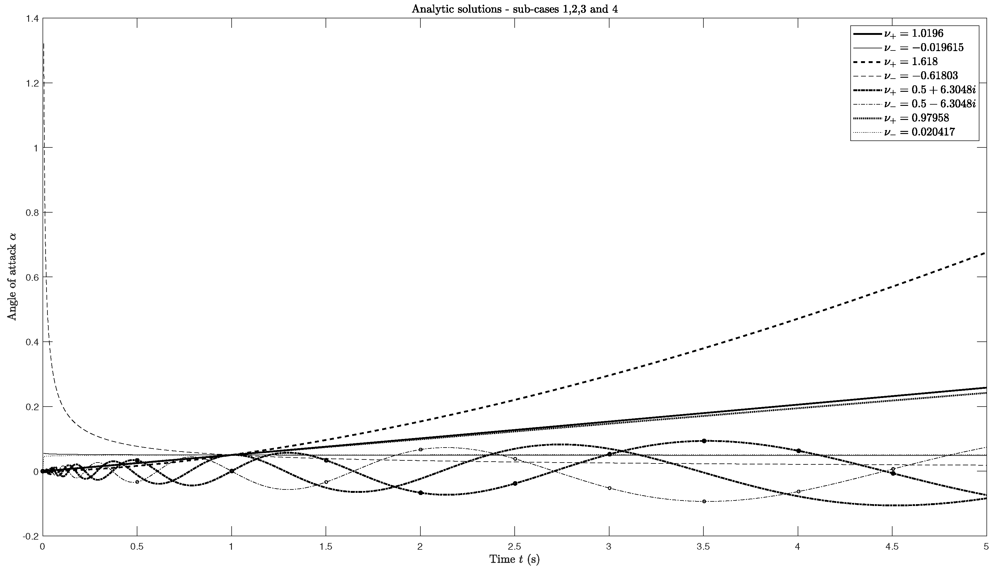
Figure 2 shows the analytic solutions for the four previous cases of the roots ${\nu }_{+}$ and ${\nu }_{-}$ of the term in square brackets in Equation (33). The four cases in Figure 2 correspond to the next four values of $\overline{ϵ}$: $-100$, $-2$, $0.05$ and 100. In the first case, when $\overline{ϵ}\ll -8$, the two roots ${\nu }_{+}$ and ${\nu }_{-}$ tend to be equal to the first two roots calculated from (33), specifically $\nu =0$ and $\nu =1$. In the third case, when $0<\overline{ϵ}<8$, the two roots ${\nu }_{+}$ and ${\nu }_{-}$ are complex numbers; therefore, each one leads to two distinct solutions of $\alpha$, evaluated from (32), one associated with the real part and the other with the imaginary part of $\alpha$. Moreover, in the third case, when choosing the complex root ${\nu }_{+}$ or ${\nu }_{-}$, the real part of $\alpha$ is the same, whereas the imaginary part of $\alpha$ is symmetric. Both solutions are plotted in Figure 2. The existence of four possible cases is due to the competition of two different effects. The first effect is the angle of attack oscillation caused by the pitching moment (9c); in aeronautics, this effect is known as the short period mode. The second competing effect is due to the balance of forces, given by Equations (9a) and (9b), and corresponds to the phugoid mode in aeronautics. The relative importance of the two effects is specified only by the dimensionless parameter defined in Equation (34). An example for the four sub-cases is provided in Figure 2. In most cases, the positive root solution ${\nu }_{+}$ from Equation (36) leads to a faster mode (the angle of attack increases faster) than with the negative root ${\nu }_{-}$.

The power type solutions for the angle of attack (32) with exponents (36) are given by

$${\alpha }_{\pm }\left(t\right)=A{t}^{{\nu }_{\pm }},$$

(38)

lead for the relative velocity (10) to:

$$\begin{array}{cc}{V}_{\pm }\left(t\right)\hfill & =\sqrt{\frac{2I{\ddot{\alpha }}_{\pm }}{\rho Sl{\alpha }_{\pm }{C}_{M_{\alpha }}}}=\frac{1}{t}\sqrt{\frac{2I{\nu }_{\pm }\left({\nu }_{\pm }-1\right)}{\rho Sl{C}_{M_{\alpha }}}}=\frac{1}{t}\sqrt{-\frac{4I}{\rho Sl{C}_{M_{\alpha }}\overline{ϵ}}}\hfill \\ \hfill & =\frac{2}{t{C}_{D_0}}\sqrt{\frac{I}{\rho Slϵ}}=\frac{2}{t{C}_{D_0}}\frac{m}{\rho S}=\frac{2}{t{C}_{D_0}}\frac{l}{\mu },\hfill \end{array}$$

(39)

where Equations (30b), (38), (35), (34), (26) and (12b) were used successively in the last relations. The rate of change with time of the relative flight path angle (28) is given by:

$$\begin{array}{cc}\hfill {\dot{\delta }}_{\pm }\left(t\right)& =C_{L_{\alpha }}\sqrt{\frac{ϵ{\alpha }_{\pm }{\ddot{\alpha }}_{\pm }}{2C_{M_{\alpha }}}}=C_{L_{\alpha }}A\sqrt{\frac{ϵ{\nu }_{\pm }\left({\nu }_{\pm }-1\right)}{2C_{M_{\alpha }}}}{t}^{{\nu }_{\pm }-1}\hfill \\ \hfill & =C_{L_{\alpha }}A\sqrt{-\frac{ϵ}{C_{M_{\alpha }}\overline{ϵ}}}{t}^{{\nu }_{\pm }-1}=\frac{C_{L_{\alpha }}}{C_{D_0}}A{t}^{{\nu }_{\pm }-1},\hfill \end{array}$$

(40)

where Equations (30a), (30b), (38), (35) and (34) are successively applied in the last relations. The integration of the last equation leads to the flight path angle as a function of time:

$${\delta }_{\pm }\left(t\right)-{\delta }_{\pm }\left(0\right)=\frac{A}{{\nu }_{\pm }}\frac{C_{L_{\alpha }}}{C_{D_0}}{t}^{{\nu }_{\pm }},$$

(41)

where ${\delta }_{\pm }\left(0\right)$ is the initial value.

The four cases (Equations (37a) to (37c)) are considered next in turn. The case from Equation (37a) leads to ${\nu }_{+}=1$ and ${\nu }_{-}=0$, which are the parabolic ballistic trajectories considered previously. In all remaining cases, the velocity (39) diverges for zero time:

$$V_{\pm }\left(0\right)=\underset{t\to 0}{lim}{V}_{\pm }\left(t\right)=\infty ,$$

(42a)

and decays to zero for a long time:

$$V_{\pm }\left(\infty \right)=\underset{t\to \infty }{lim}{V}_{\pm }\left(t\right)=0.$$

(42b)

The angle of attack (38) and variation of the flight path angle (41) scale similarly with time: (i) in the case (37b) leading to

$$\begin{array}{c}\hfill {\alpha }_{+}\left(0\right)={\alpha }_{-}\left(\infty \right)=0,\end{array}$$

(43a)

$$\begin{array}{c}\hfill {\alpha }_{+}\left(\infty \right)={\alpha }_{-}\left(0\right)=\infty ;\end{array}$$

(43b)

(ii) in the case (37d) leading to

$$\begin{array}{c}\hfill {\alpha }_{\pm }\left(0\right)=0,\end{array}$$

(44a)

$$\begin{array}{c}\hfill {\alpha }_{\pm }\left(\infty \right)=\infty .\end{array}$$

(44b)

In both cases, the angle of attack (and also the flight path angle) vary monotonically with time; that is, the body rotates as it falls along a modified parabolic trajectory.

In the case from Equation (37c), the roots

$$\begin{array}{c}\hfill {\nu }_{\pm }=\frac{1}{2}\pm \mathrm{i}\omega ,\end{array}$$

(45a)

$$\begin{array}{c}\hfill \omega ={\left|\frac{2}{\overline{ϵ}}-\frac{1}{4}\right|}^{1/2},\end{array}$$

(45b)

lead to oscillations of the angle of attack:

$${\alpha }_{\pm }\left(t\right)=A{t}^{1/2}{\mathrm{e}}^{\pm \mathrm{i}\omega lnt},$$

(46)

whose amplitude is zero initially:

$${\alpha }_{\pm }\left(0\right)=0,$$

(47a)

and diverges for a long time:

$$\left|{\alpha }_{\pm }\left(\infty \right)\right|=\infty .$$

(47b)

The oscillation frequency (45b) vanishes in the transition $\overline{ϵ}=8$ to the monotonic case (37d). The real solutions corresponding to (46) are the real and imaginary parts:

$$\begin{array}{cc}\hfill {\alpha }_1\left(t\right)& =\mathrm{Re}\left\{{\alpha }_{\pm }\left(t\right)\right\}=A\sqrt{t}cos\left(\omega lnt\right),\hfill \end{array}$$

(48a)

$$\begin{array}{cc}\hfill {\alpha }_2\left(t\right)& =\mathrm{Im}\left\{{\alpha }_{\pm }\left(t\right)\right\}=\pm A\sqrt{t}sin\left(\omega lnt\right).\hfill \end{array}$$

(48b)

In this case, the motion involves an oscillation in the angle of attack as the body falls.

Thus, the analytic solutions, although valid only for small angles of attack, show the existence of two regimes of fall depending on the parameter (34) and (26):

$$\overline{ϵ}=-\frac{C_{D_0}^2}{C_{M_{\alpha }}}\frac{\rho Sl}{m}{\left(\frac{r}{l}\right)}^2>0.$$

(49)

If the parameter (49) is large (37d), the tumbling body rotates as it falls (Figure 3a); this corresponds to a predominance of the phugoid mode. If the parameter (49) is small (37c), the tumbling body oscillates as it falls (Figure 3b); this corresponds to the predominance of the short-period mode. A simple analogy [8] is the motion of a circular pendulum of mass m, length s in the gravity field g, for which the difference in potential energy between the lowest $\theta =0$ and highest $\theta =\pi$ points is:

$$E_0=2mgs.$$

(50a)

The total energy of the pendulum, comprising both kinetic and potential components, is given by

$$E=\frac{1}{2}m{s}^2{\dot{\theta }}^2-mgscos\theta =\mathrm{const},$$

(50b)

and remains conserved. This leads to three cases: (i) if the total energy (50b) is less than the difference in potential energy between top and bottom (50a), $E<E_0$, the pendulum cannot reach the top, the pendulum motion is oscillatory (Figure 4b), similar to the short-period mode of aircraft, and the oscillating fall of tumbling body (Figure 3b); (ii) if the total energy (50b) is larger than the difference in potential energy between top and bottom (50a), $E>E_0$, the pendulum goes through the top with non-zero velocity, the pendulum motion is circulatory (Figure 4a), corresponds to the phugoid mode of aircraft and to the rotating fall of a tumbling body (Figure 3a); (iii) in the intermediate border line case of total energy (50b) equal to the difference (50a) of potential energy at the top and bottom, $E=E_0$, the pendulum would stop at the top, corresponding to $\overline{ϵ}=8$ in (36), leading to ${\nu }_{\pm }=1/2$, while the angle of attack (32) and flight path angle (41) both increase with time as local velocity (39) decreases.

Since the differential Equation (31) for small angles of attack is non-linear, the principle of superposition does not hold and a linear combination of the solutions from Equations (38) or (46) is generally not a solution. Since the analytic solutions are restricted to small angles of attack, the limits of Equations (43a), (44b) and (47b) hold only for small values. However, the existence of monotonic rotation and oscillatory solutions is confirmed by the numerical solutions (Section 5) that hold for unrestricted angles of attack.

5. Generic Numerical Simulations

5.1. Numerical Model

In order to have a solution for the trajectory of the rocket for the full spectrum of angles of attack, it is necessary to use a numerical method. The model requires initial conditions that must be consistent with the initial positions and velocities in free fall coordinates. The initial position is specified in Earth-fixed coordinates:

$$\begin{array}{cc}\hfill X\left(0\right)& =x_0,\hfill \end{array}$$

(51a)

$$\begin{array}{cc}\hfill Z\left(0\right)& =z_0,\hfill \end{array}$$

(51b)

and thus, according to (2a) and (2b), the origin in free fall coordinates is given by

$$\begin{array}{cc}\hfill x\left(0\right)& =0,\hfill \end{array}$$

(51c)

$$\begin{array}{cc}\hfill z\left(0\right)& =0.\hfill \end{array}$$

(51d)

The initial velocity (5a) and (5b) in Earth-fixed coordinates is given as follows:

$$\begin{array}{cc}\hfill \dot{X}\left(0\right)& =U_{0}cos{\gamma }_0,\hfill \end{array}$$

(52a)

$$\begin{array}{cc}\hfill \dot{Z}\left(0\right)& =U_{0}sin{\gamma }_0,\hfill \end{array}$$

(52b)

This equation is consistent with the total velocity in Earth-fixed coordinates (4a):

$$U_0={\left|{\left[\dot{X}\left(0\right)\right]}^2+{\left[\dot{Z}\left(0\right)\right]}^2\right|}^{1/2}.$$

(52c)

In free fall coordinates the initial horizontal and vertical velocities

$$\begin{array}{cc}\hfill \dot{x}\left(0\right)=\dot{X}\left(0\right)& =U_{0}cos{\gamma }_0,\hfill \end{array}$$

(53a)

$$\begin{array}{cc}\hfill \dot{z}\left(0\right)=\dot{Z}\left(0\right)& =U_{0}sin{\gamma }_0,\hfill \end{array}$$

(53b)

are assumed to equal those, (52a) and (52b), in Earth-fixed coordinates, which is consistent with (3a) and (3b) for

$$\begin{array}{cc}\hfill u_0& =0,\hfill \end{array}$$

(53c)

$$\begin{array}{cc}\hfill v_0& =0.\hfill \end{array}$$

(53d)

It follows that the initial total velocity is the same in Earth-fixed (4a) and free fall (4c) coordinates:

$$V_0={\left|{\left[\dot{x}\left(0\right)\right]}^2+{\left[\dot{z}\left(0\right)\right]}^2\right|}^{1/2}={\left|{\left[\dot{X}\left(0\right)\right]}^2+{\left[\dot{Z}\left(0\right)\right]}^2\right|}^{1/2}=U_0.$$

(54)

The initial conditions include the angle of attack (29a), and its first (29b) and second (29c) time derivatives, the latter involving the total initial velocity $V_0$ in free fall coordinates, which are required to solve the angle of attack differential Equation (27); the angle of attack specifies the relative velocity by (10). The initial relative flight path angle ${\delta }_0$ (value of $\delta$ at initial time), with $u_0=0=v_0$, is equal to ${\gamma }_0$ (value of $\gamma$ at initial time) and is needed to solve the flight path angle differential Equation (28). The third-order time derivative of the angle of attack at time zero is obtained from (13) using (19), (22) and (25):

$$\begin{array}{c}\hfill \stackrel{⃛}{\alpha }-2\dot{\alpha }\ddot{\alpha }\frac{cos\left(2\alpha \right)}{sin\left(2\alpha \right)}=-C_D\left(\alpha \right){\ddot{\alpha }}^{3/2}\sqrt{\frac{4\mu {\epsilon }_0}{C_{M_{\alpha }}sin\left(2\alpha \right)}}\end{array}$$

(55a)

and also (26) for $t=0$:

$$\begin{array}{c}\hfill \frac{1}{2}sin\left(2{\alpha }_0\right){\stackrel{⃛}{\alpha }}_0={\dot{\alpha }}_0{\ddot{\alpha }}_{0}cos\left(2{\alpha }_0\right)-C_D\left({\alpha }_0\right)\sqrt{\frac{ϵ}{C_{M_{\alpha }}}{\ddot{\alpha }}_0^{3}sin\left(2{\alpha }_0\right)}.\end{array}$$

(55b)

where ${\stackrel{⃛}{\alpha }}_0$ is the value of $\stackrel{⃛}{\alpha }$ for $t=0$. Each root in the above equation corresponds to a distinct solution. These two solutions will be compared in Section 6. The first-order time derivative of the flight path angle at time zero is a particular case of Equation (28):

$${\dot{\delta }}_0\equiv \dot{\delta }\left(0\right)=C_L\left({\alpha }_0\right)\sqrt{\frac{ϵ{\ddot{\alpha }}_0}{2C_M\left({\alpha }_0\right)}}.$$

(56)

Thus, six independent initial conditions are required: (i–ii) two initial positions (51a) and (51b); (iii–iv) initial flight path angle and velocity components in Earth reference (52a) and (52b); (v–vi) initial angle of attack and its first-order time derivative (29a) and (29b). All other initial conditions follow from the preceding six: (vii–viii) the initial horizontal and vertical velocities in free fall coordinates from (53a) and (53b); (ix) the initial first-order time derivative of the relative flight path angle from (56); (x) the initial third-order time derivative of the angle of attack from (55b). The solution of the Equations of motion for the flight path is made following the next steps: (xi) integrating (27) for the angle of attack with initial conditions (29a) and (29b); (xii) (10) follows the velocity in free fall coordinates; (xiii) integration of (28) with the initial condition specifies the flight path angle; (xiv) the total velocity follows from (7b), (53c) and (53d) as follows:

$$U\left(t\right)=-gtsin\gamma \pm {\left|{\left[V\left(t\right)\right]}^2-{\left(gtcos\gamma \right)}^2\right|}^{1/2};$$

(57)

(xv) integration of (5a) and (5b) with initial conditions (51a) and (51b) specifies the flight path in Earth-fixed coordinates; (xvi) substitution in (2a) and (2b) with (53c) and (53d) specifies the trajectory in the free fall coordinates:

$$\begin{array}{c}\hfill x\left(t\right)=X\left(t\right)-x_0,\end{array}$$

(58)

$$\begin{array}{c}\hfill z\left(t\right)=Z\left(t\right)-z_0+\frac{1}{2}g{t}^2.\end{array}$$

(59)

The coefficients involve the following: (xvii–xix) the lift (17), the drag (23) and pitching moment (19) coefficients that depend only on the angle of attack and make the third-order differential equation for the angle of attack (27) more strongly non-linear; (xx) the atmospheric density $\rho$ and hence the rocket parameter (26) that depend on altitude Z in the Earth-fixed reference frame (xv) and render the whole problem implicit, because it appears in (xi). To implement the numeric model, a computational tool was built using the MATLAB software [9]. The program is split into three phases: read user inputs, integration process and data treatment.

5.2. Read Input Data

The choice of tumbling body for numerical simulation could be (i) debris from an explosion, or (ii) a spent rocket stage or (iii) the complete rocket after a propulsion failure. While, historically, multiple (i) rocket explosions have occurred, either by accident or command, there is a shortage of precise data on debris mass, shape, initial velocity, angle of attack and other properties as well as some derivatives to apply the model. In any case, (i) small debris would not travel as far as (ii) a spent rocket stage or (iii) the complete rocket with most propellant unused after a propulsion failure shortly after lift-off. The last, (iii) worst case scenario is chosen as a numerical example for the Ariane 5 rocket.

During the “read user inputs” phase, the program reads the values chosen by the user for the six initial conditions required for the numeric integration as well as the values of the seven rocket parameters [10]. The rocket parameters are as follows: rocket mass, radius, height or lengthscale l, distance between center of mass and center of pressure a, slope of the lift coefficient $C_{L_{\alpha }}$, friction drag $C_{D_0}$ and lift to drag proportionality constant K. The default rocket configuration contains values from the Ariane 5 rocket [11], which are presented in

Table 1. Ariane 5 rocket data [10,11].

Parameter	Value
Mass m (kg)	780,000
Radius R (m)	2.7
Height l (m)	50.5
Distance a (m)	−1.5
$C_{L_{\alpha }}$	0.0955
$C_{D_0}$	0.05
K	1.24

.

The radius of gyration in pitch for a homogeneous cylinder of radius R and length l is given by [12]

$$r_1=\sqrt{\frac{R^2}{4}+\frac{l^2}{12}},$$

(60)

corresponding to the extreme case of a rocket full of propellant. The opposite extreme case of propellant exhausted corresponds to a hollow cylindrical shell of radius R and length l, for which the transverse or pitch radius of gyration is given by [12]

$$r_2=\sqrt{\frac{R^2}{2}+\frac{l^2}{12}}.$$

(61)

The calculations use the geometric mean

$$r=\sqrt{r_1{r}_2}=\sqrt[4]{\frac{R^2}{8}+\frac{l^4}{144}+\frac{R^2{l}^2}{24}},$$

(62)

for the radius of gyration in pitch of a cylindrical rocket with a partial propellant load.

5.3. Integration Method

This entire phase works in a loop cycle, i.e., the program uses the rocket data and the six variables with initial conditions at any point in time $t_n$ to obtain new conditions at the next point in time $t_{n+1}$ with n being any value between 0 and the total number of cycles.

Before performing the numeric integration itself, the third derivative of the angle of attack, flight path angle derivative, and the X and Z derivatives must be calculated. The steps taken in the loop by the program to obtain all the derivatives are as follows:

• Calculate all the aerodynamic coefficients from Equations (17), (19) and (23);
• Calculate the air density (using a model explained later) and the modulus of the relative velocity using Equation (10);
• Obtain the value of all the required derivatives using one of the solutions of the quadratic Equation (27) with respect to $\stackrel{⃛}{\alpha }$ and using Equations (28), $\dot{x}=Vcos\delta$ and $\dot{z}=Vsin\delta$; the trajectory in Earth reference is then evaluated from (2a) and (2b); alternatively, to obtain the derivatives $\dot{x}$ and $\dot{z}$, one can find a solution $\left\{\dot{X},\dot{Z}\right\}$ from Equations (4d) and (6c), considering that $Ucos\gamma =\dot{X}$ and $Usin\gamma =\dot{Z}$, and then use the relations (3a) and (3b).

In the third step, the air density is calculated from the altitude of the rocket in an Earth-fixed reference frame. There are several models of the variation of the air density with the altitude; for this work, the USSA76 density model is employed. This model assumes that the atmosphere is a spherically symmetric 1000 km thick gaseous shell surrounding the Earth. The methodology used to model the atmospheric density can be found in [13].

Concerning the numeric integration itself, the first step is to choose an integrating function. This is particularly important in this work, not only because different integrating functions have different inherent numeric errors, but also because the Equations used to calculate the rocket velocity (10) and to calculate the third derivative of the angle of attack (13) have indeterminations whenever the angle of attack tends to $0°$, $90°$, $180°$ or $270°$.

In order for the integration to be made without incurring in a large error induced by the aforementioned indetermination, the integrating function must be chosen carefully. This is seen in Figure 5, which shows the rocket velocity distribution over time (since it is directly affected by the indetermination, it is a good error indicator) using the same initial conditions and rocket data for four different integrating functions present in MATLAB software: ODE45, ODE113, ODE15s and ODE23s.

Figure 5 shows that all the four integrators lead to similar results in the velocity and, therefore, in the fall trajectory of the tumbling body. Moreover, the velocity has a smooth variation and does not have any sudden peaks/spikes (that can occur due to an indetermination), independently of the chosen integrator. However, the ODE23s integrator provides the worst results, since during the integration process, the intermediate matrices to solve the problem numerically can be close to singular or badly scaled. The ODE23s function is a single step solver (only needs the solution at the immediately preceding time point) based on a modified Rosenbrock formula of order 2 [9]. Moreover, the ODE113 integrator shows a sudden variation in the value of velocity during the simulation. Therefore, the ODE45 integrator is the selected function because it performs well with this differential equations problem; in other words, it is able to solve the problem and is not slow (that is an indicator that this problem might not exhibit stiffness since ODE45 is a non-stiff solver and does not have difficulties solving it; if the ODE45 method was inefficient, the ODE15s integrator would be chosen to solve the differential equations, being a better alternative to stiff problems). The ODE45 integrator is also a single-step solver, in this case, based on an explicit Runge–Kutta (4, 5) formula, the Dormand–Prince pair [9].

5.4. Data Analysis

In the final phase of the program, the values of time, angle of attack, flight path angle and other variables can be stored in arrays so that all data can be presented in the form of plots. In the Section 6 only the trajectories are shown as functions of several parameters.

6. Effect of Initial Conditions

6.1. Analysis of Two Baseline Configurations

To test the MATLAB tool, it is necessary to first choose a baseline configuration containing all the initial conditions and rocket data. After the start of testing, it was found that the rocket can have two different full modes, namely, an oscillatory mode (OM) and a rotation mode (RM). For this reason, two base configurations are required. Both base configurations use the Ariane 5 rocket data, indicated in Table 1, and the set of initial conditions as summarized in

Table 2. Base configuration.

Initial Conditions		Rocket Data
${\alpha }_0$	$85°$ or $5°$	Mass m (kg)	780,000
${\dot{\alpha }}_0$	0.5 $°$/s	Radius R (m)	2.7
$U_0$	150 m/s	Height l (m)	50.5
${\gamma }_0$	$80°$	Distance a (m)	$-1.5$
$X\left(0\right)$	$0\mathrm{m}$	$C_{L_{\alpha }}$	0.0955
$Z\left(0\right)$	$2000\mathrm{m}$	$C_{D_0}$	0.05
Time	$200\mathrm{s}$	K	1.24
$t_{\mathrm{step}}$	$1\mathrm{s}$	$I\left(\mathrm{kg}{\mathrm{m}}^2\right)$	$1.67\times {10}^8$
		$S\left({\mathrm{m}}^2\right)$	22.9

.

The configuration with the angle of attack of $85°$ will be named the first configuration and the one with the angle of attack of $5°$ the second configuration.

In Figure 6 and Figure 7, the differences in trajectory and angle variations are shown over the time for both configurations. To differentiate results obtained with the positive root and negative root when using Equation (55b) (obtained with plus and minus sign before the square root respectively, although in Equation (55b) only the negative sign is shown before the term that is multiplied by the square root), an asterisk mark (${}^{*}$) will be presented whenever a result was obtained using the negative root. Both solutions can be obtained from the quadratic Equation (27) with respect to $\stackrel{⃛}{\alpha }$ to compare the results obtained in Section 6 with the analytic solutions obtained in Section 4.

In terms of trajectory, as can be seen in Figure 6, contrasting results are obtained for each configuration/root combination. Using the first configuration combined with the negative root solution leads to the longest range while using the first configuration with the positive root solution leads to the shortest range. Using the second configuration leads to the two intermediate ranges; however, in this instance, the use of the negative root leads to the largest range of the two. Therefore, it is possible to conclude, at least for this particular example, that the negative root solution will help a rocket falling not only in RM but also in OM motions to obtain larger ranges of the rocket.

In terms of angle variations, the two fall modes are shown in Figure 7: in the OM, plotted in configuration 2, the rocket oscillates around $0°$ (nevertheless, Figure 7 does not show the variation around $0°$ because the rocket reaches the ground—$Z=0\mathrm{m}$—before it performs a complete oscillation) and in the RM; regarding the configuration 1, the rocket increases the value of the angle of attack monotonically. The relative flight path angle is nearly constant during the entire simulation. This can be explained by recalling the flight path angle derivative expression (28). The derivative is proportional to the square root of the dimensionless parameter, which will always be much smaller than 1 (the rocket mass is much larger than any of the remaining terms).

By observing Figure 7, the thick solid line is superimposed on the thin solid line while the thick dash-dotted line is superimposed on the thin dash-dotted line. This means that using the first or the second solution for $\stackrel{⃛}{\alpha }$ does not change the fall mode, but it changes the speed of the mode. As already concluded in Figure 6, using the negative root solution leads to a slightly faster RM and to a slightly faster OM, at least for this particular example. This conclusion may not hold for other initial conditions and rocket data.

The existence of two modes and their different speeds are in agreement with the predictions from the analytical analysis detailed in Section 4.

6.2. Sensitivity Analysis

Using the base configurations, a sensitivity analysis is performed to every initial condition (Section 6) and rocket parameter (Section 7) with the purpose of understanding their influence in the trajectory of the tumbling body and in specifying the fall mode.

The initial angle of attack influences mostly the fall mode as is shown in

Table 3. Sensitivity analysis to the angle of attack.

${\mathit{\alpha }}_{\mathbf{0}}\left(°\right)$	Mode	$\mathit{\alpha }\left(°\right)$	$\ddot{\mathit{\alpha }}\left(\mathbf{rad}/{\mathbf{s}}^2\right)$
85	RM	–	$-5.8\times {10}^{-5}$ to $7.6\times {10}^{-5}$
75	RM	–	$-5.1\times {10}^{-5}$ to $6.8\times {10}^{-5}$
65	RM	–	$-7.8\times {10}^{-5}$ to $6.5\times {10}^{-5}$
50	RM	–	$-1.0\times {10}^{-4}$ to $-6.6\times {10}^{-7}$
45	RM	–	$-1.0\times {10}^{-4}$ to $-3.2\times {10}^{-5}$
30	RM	–	$-9.5\times {10}^{-5}$ to $-5.3\times {10}^{-5}$
15	OM ($T=1492\mathrm{s}$)	$15.00$ to $43.54$	$-8.6\times {10}^{-5}$ to $-4.9\times {10}^{-5}$
5	OM ($T=1686\mathrm{s}$)	$5.00$ to $40.27$	$-8.2\times {10}^{-5}$ to $-1.8\times {10}^{-5}$
$-5$	OM ($T=1793\mathrm{s}$)	$-5.00$ to $40.56$	$-8.1\times {10}^{-5}$ to $1.8\times {10}^{-5}$
$-65$	RM	–	$-4.8\times {10}^{-5}$ to $7.8\times {10}^{-5}$
$-115$	RM	–	$-7.8\times {10}^{-5}$ to $1.1\times {10}^{-5}$

. An initial angle of attack near $90°$ favours the RM while an angle closer to $0°$ favours the OM. The period of the oscillations increases as the initial angle of attack decreases; however, when the initial angle deviates greatly from $0°$, the mode of fall becomes RM instead of OM. The results are different for symmetric angles of attack, and are also different, but quite similar, if the difference between two angles is $\pm 180°$.

Similar to the angle of attack, the initial angular velocity also affects the fall mode. The results for this initial condition are presented in

Table 4. Sensitivity analysis to the angular velocity.

${\mathit{\alpha }}_0\left(°\right)$	${\dot{\mathit{\alpha }}}_0\left(°/\mathbf{s}\right)$	Mode	$\dot{\mathit{\alpha }}\left(\mathbf{rad}/\mathbf{s}\right)$
85	$-1$	RM	$-0.022$ to $-0.018$
85	$-0.5$	RM	$-0.016$ to $-0.009$
85	0	RM	$-0.005$ to $0.000$
85	0.5	RM	$0.009$ to $0.015$
85	1	RM	$0.017$ to $0.022$
85	2	RM	$0.035$ to $0.040$
5	$-1$	RM	$-0.018$ to $-0.012$
5	$-0.5$	OM ($T=554\mathrm{s}$)	$-0.009$ to $-0.001$
5	0	OM ($T=488\mathrm{s}$)	$-0.001$ to $0.000$
5	0.5	OM ($T=1685\mathrm{s}$)	$-0.005$ to $0.009$
5	1	RM	$0.011$ to $0.018$
5	2	RM	$0.032$ to $0.035$

. A sufficiently high/low initial angular velocity is enough to change the initial fall mode of either configuration, but the change is more likely to occur for a smaller initial angle of attack. Larger initial angular velocities in modulus lead to faster revolution cycles or larger periods of oscillation depending on the fall mode.

The initial rocket velocity has an effect on both fall mode and trajectory. Regarding the effect on the fall mode, from

Table 5. Sensitivity analysis to the initial velocity.

${\mathit{\alpha }}_0\left(°\right)$	${\mathit{U}}_0\left(\mathbf{m}/\mathbf{s}\right)$	Mode	$\mathit{\alpha }\left(°\right)$
85	110	RM	–
85	130	RM	–
85	150	RM	–
85	170	RM	–
85	190	RM	–
5	110	RM	–
5	130	RM	–
5	150	OM ($T=1685\mathrm{s}$)	$-5.00$ to $40.27$
5	170	OM ($T=880\mathrm{s}$)	$-5.00$ to $34.59$
5	190	OM ($T=653\mathrm{s}$)	$-0.441$ to $30.42$

, for larger velocities, the amplitude and period of oscillation are lower.

In terms of trajectory, as expected, larger initial velocities lead to the rocket travelling farther, as seen in Figure 8.

Both the flight path angle and initial position have no impact on the fall mode. The flight path angle is nearly constant throughout the entire simulation and only changes the direction of the trajectory, as shown in Figure 9. As for the initial coordinates $X\left(0\right)$ and $Z\left(0\right)$, they simply change the trajectory point of origin since the change in density value is not enough to significantly influence the other flight parameters.

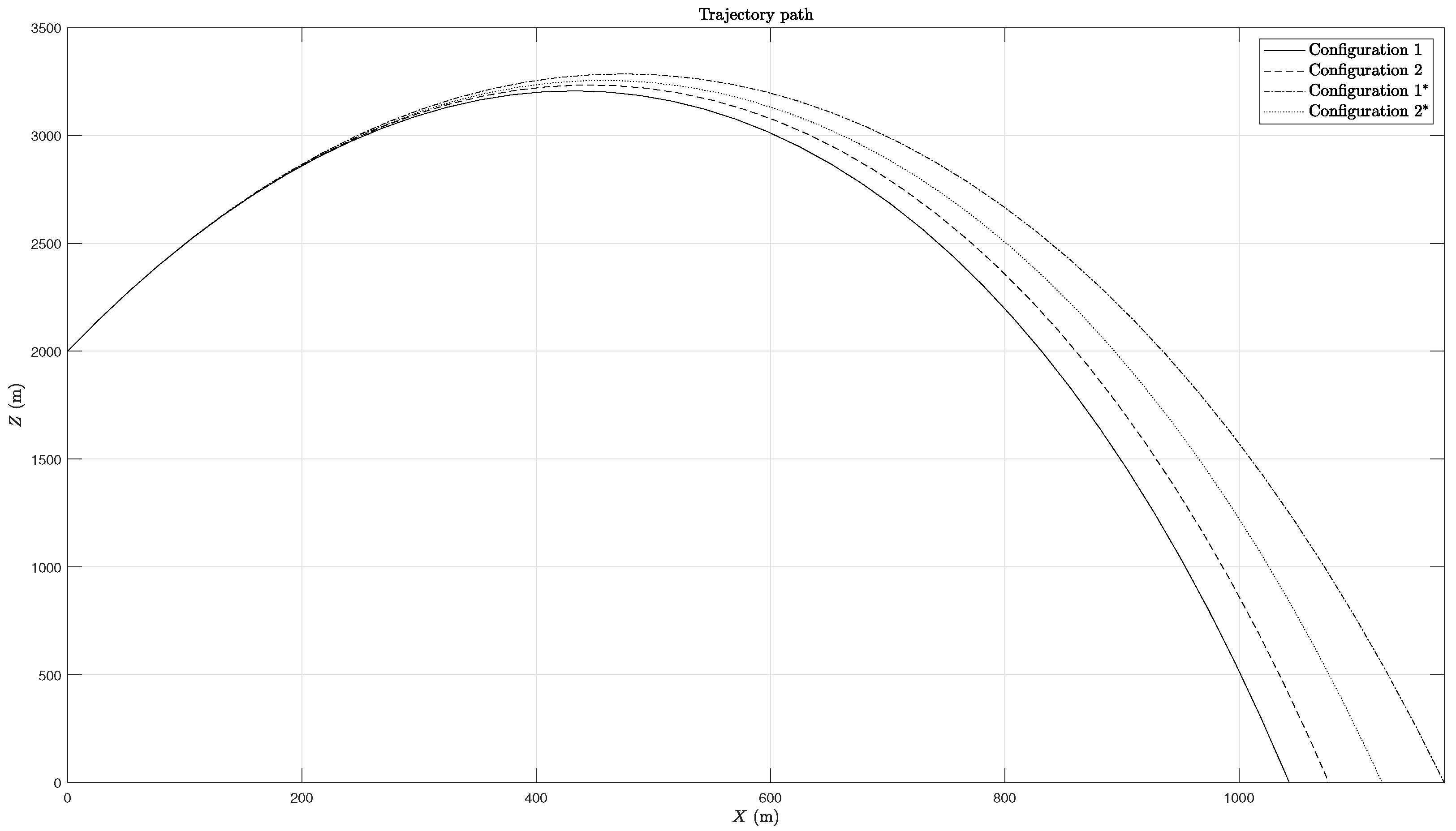
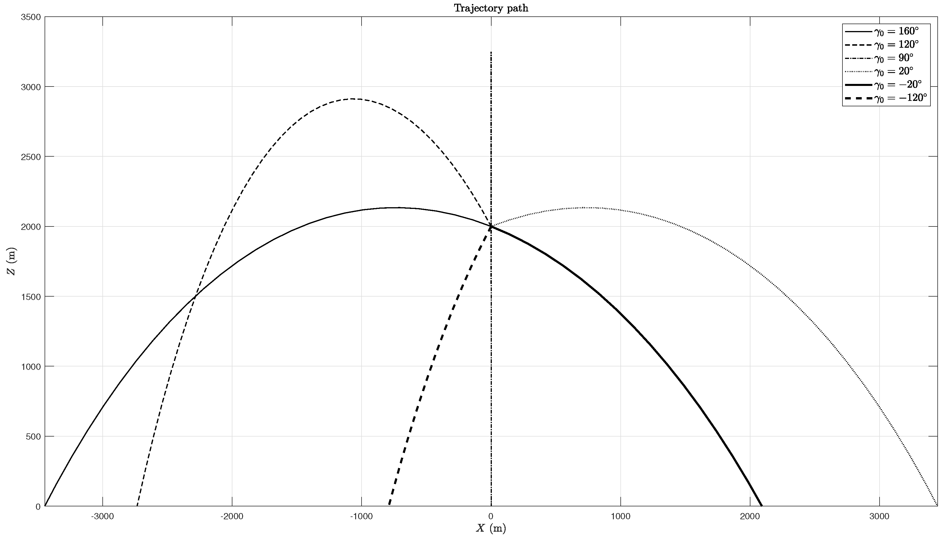
7. Effect of the Rocket Parameters

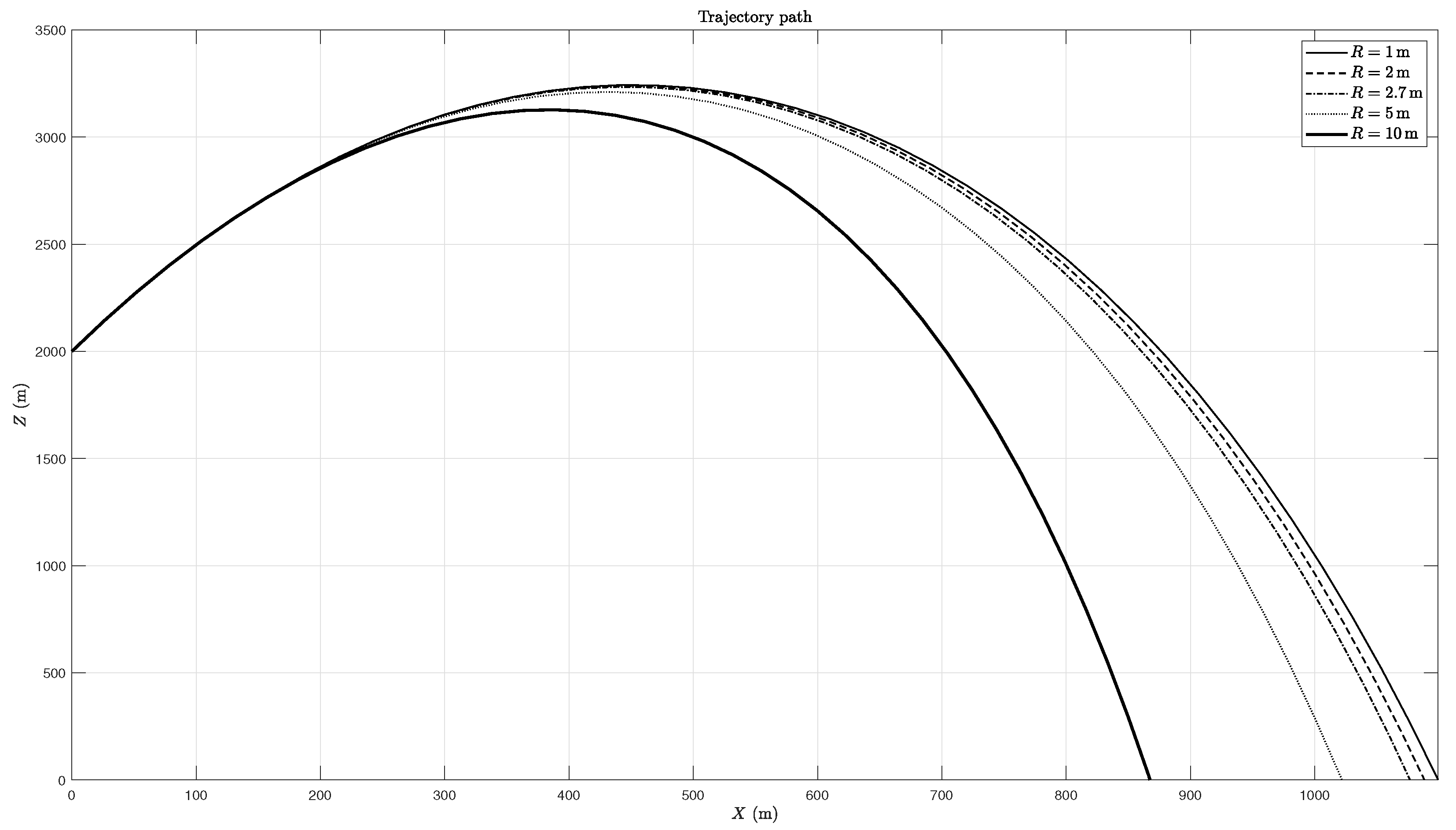
Proceeding to the sensitivity analysis of the effects of the rocket parameters, the rocket mass was found to have a direct influence in both trajectory and fall mode. In terms of fall mode, smaller masses lead to smaller periods and amplitudes of oscillation, as is shown in

Table 6. Sensitivity analysis to the rocket mass using the second configuration.

Mass (kg)	Mode	$\mathit{\alpha }\left(°\right)$	$\mathit{\delta }\left(°\right)$
5000	OM ($T=101\mathrm{s}$)	$-7.31$ to $10.55$	$78.65$ to $82.83$
10,000	OM ($T=113\mathrm{s}$)	$-7.84$ to $10.26$	$79.08$ to $81.92$
50,000	OM ($T=199\mathrm{s}$)	$-12.28$ to $11.51$	$79.56$ to $81.07$
100,000	OM ($T=292\mathrm{s}$)	$-16.23$ to $14.23$	$79.75$ to $81.09$
780,000	OM ($T=1685\mathrm{s}$)	$-5.00$ to $40.27$	$80.00$ to $80.94$
1,500,000	RM	–	$80.00$ to $80.51$

, which was obtained using the second configuration. For an extremely heavy body, the period of oscillations is so large that the fall mode becomes RM. Using the first configuration leads to the RM conclusions, independently of the mass of the tumbling body.

In terms of trajectory (Figure 10), larger masses have the longest range and the smaller masses the shortest. Larger masses are less affected by aerodynamic forces and come closer to the ballistic trajectory while lighter masses are more affected by drag and travel less far. The usual assumption that the heaviest tumbling body is usually the worst case (that travels farther) is supported by the results obtained in this analysis. The effect of mass is less significant for heavier bodies, by observing that changing the value of mass from 500,000 kg to 1,500,000 kg does not change the range as much as changing the mass from 5000 kg to 500,000 kg.

Smaller masses also have a second effect other than reducing the trajectory range, namely introducing some wobbles to the usually ballistic shaped trajectory. These wobbles are a consequence of the following: (i) the flight path angle amplitude of oscillation increasing as the mass of the rocket is reduced, which supports the explanation that the flight path angle was seemingly constant because of the large mass value; (ii) large velocity oscillations as the mass is reduced.

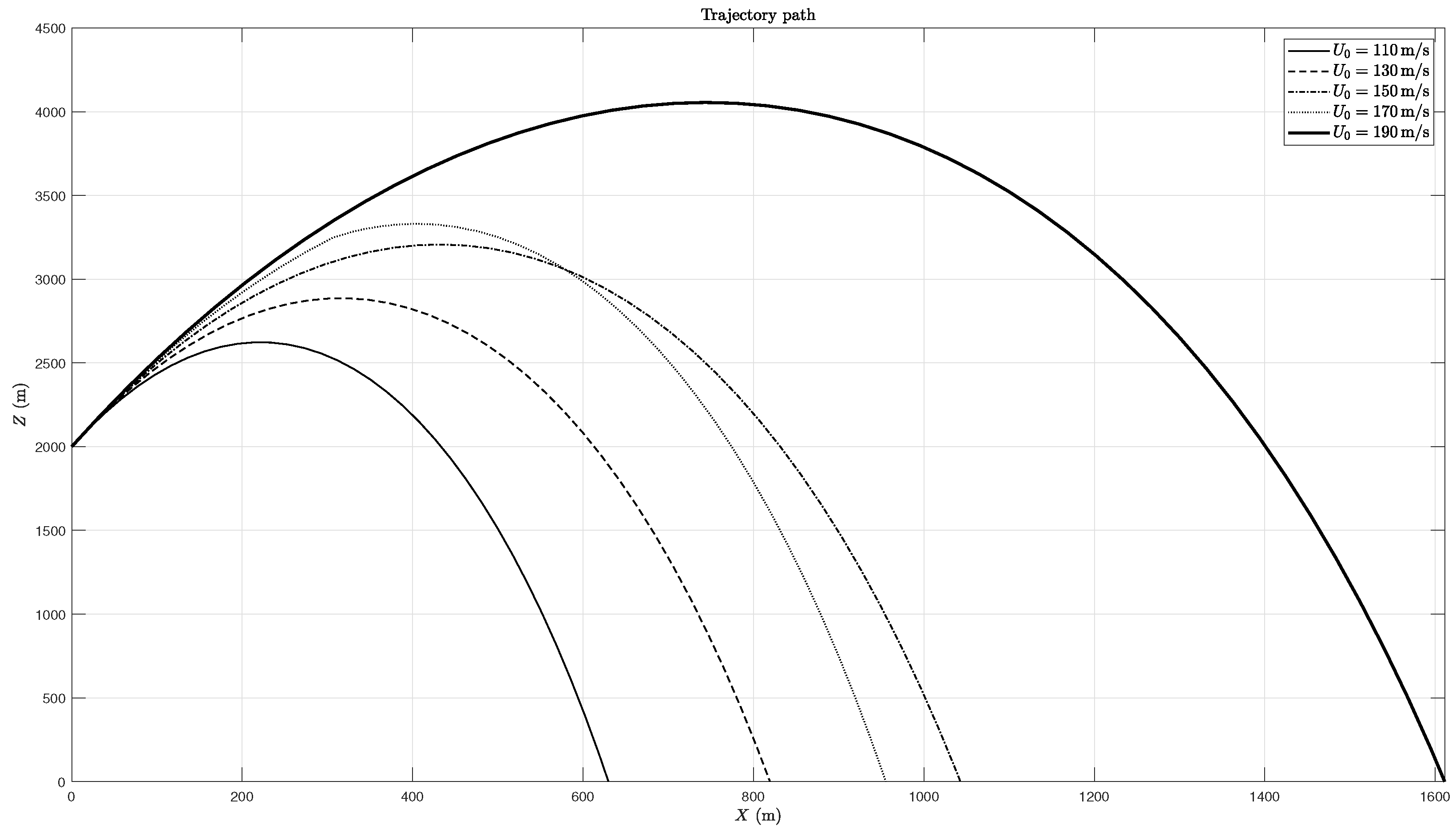
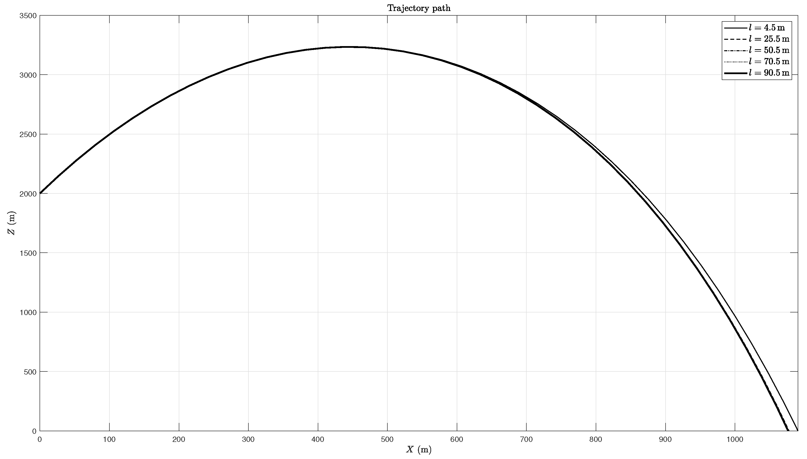
The radius of gyration of the rocket also has an effect on both the trajectory and fall mode. Smaller values of the radius of gyration usually lead to larger ranges not only when the RM is dominant (Figure 11), but also when the OM configuration is used (Figure 12). An increasing radius of gyration or moment of inertia implies greater kinetic energy of oscillation in both modes and reduces translational energy and range.

In terms of fall mode, as can be seen in

Table 7. Sensitivity analysis to the rocket radius.

${\mathit{\alpha }}_0\left(°\right)$	Radius (m)	Mode	$\mathit{\alpha }\left(°\right)$
5	1	RM	–
5	2	RM	–
5	2.7	OM ($T=1685\mathrm{s}$)	$-5.00$ to $40.27$
5	5	OM ($T=502\mathrm{s}$)	$-21.32$ to $21.24$
5	10	OM ($T=254\mathrm{s}$)	$-13.52$ to $12.00$

, larger radius of gyration values work in favour of the OM fall by reducing the amplitude of the oscillations.

The height of the rocket was found to have effects on the fall mode and trajectory, as can be seen in

Table 8. Sensitivity analysis to the rocket height.

${\mathit{\alpha }}_0\left(°\right)$	Length (m)	Mode	$\mathit{\alpha }\left(°\right)$
5	4.5	OM ($T=63\mathrm{s}$)	$\pm 7.11$
5	25.5	OM ($T=271\mathrm{s}$)	$-20.18$ to $19.22$
5	50.5	OM ($T=1685\mathrm{s}$)	$-5.00$ to $40.27$
5	70	RM	–
5	90.5	RM	–

and in Figure 13 and Figure 14. In terms of the fall mode, having a larger height will favour the RM. Increasing the height of the rocket maintaining the mass constant is the same as increasing only the moment of inertia of the rocket; therefore, a larger moment of inertia leads to a stronger tendency to rotate.

In terms of trajectory, the variation to the height of the rocket will lead to the same range changes as the increase of the gyration radius since both parameters contribute to calculating the inertia of the rocket.

The distance between the centre of pressure and centre of mass is very important toward determining the fall mode. The results of

Table 9. Sensitivity analysis on the distance between the center of pressure and center of mass.

${\mathit{\alpha }}_0\left(°\right)$	$\mathit{a}\left(\mathbf{m}\right)$	Mode	$\mathit{\alpha }\left(°\right)$
85	$-5$	RM	–
85	$-3$	RM	–
85	$-1.5$	RM	–
85	$-0.5$	RM	–
85	0.5	OM ($T=280\mathrm{s}$)	$85.00$ to $150.83$
85	1.5	OM ($T=218\mathrm{s}$)	$85.00$ to $123.02$
85	3	OM ($T=445\mathrm{s}$)	$59.50$ to $113.71$
85	5	OM ($T=168\mathrm{s}$)	$73.51$ to $108.90$
5	$-5$	OM ($T=292\mathrm{s}$)	$-21.00$ to $20.57$
5	$-3$	OM ($T=444\mathrm{s}$)	$-14.55$ to $26.74$
5	$-1.5$	OM ($T=1685\mathrm{s}$)	$5.00$ to $40.27$
5	$-0.5$	RM	–
5	0.5	OM ($T=406\mathrm{s}$)	$5.00$ to $130.12$
5	1.5	OM ($T=225\mathrm{s}$)	$5.00$ to $152.00$
5	3	RM	–
5	5	OM ($T=182\mathrm{s}$)	$5.00$ to $155.97$

are inconclusive since it is difficult to predict what the fall mode is for a certain distance a. Table 9 also shows that the fall mode is dependent on the initial angle of attack, thus predicting that there are more parameters, not depicted on Table 9, that significantly influence the fall mode.

Assuming that the initial angle of attack is close to $90°$, when the distance a is negative, the fall mode is RM, but when the sign of that distance changes, the movement becomes OM, generally with the period of the oscillation decreasing when the distance a increases. When the initial angle of attack is close to $0°$, the sign of the distance a does not predict the fall mode; nevertheless, Table 9 shows that in almost all cases the fall mode is OM.

Lastly, regarding the aerodynamic coefficients, while $C_{L_{\alpha }}$ has its most noticeable effect in the fall mode, $C_{D_0}$ and K can exert their influence on the trajectory and fall mode. Larger values of $C_{L_{\alpha }}$ decrease both the period and amplitude of oscillation as can be seen in

Table 10. Sensitivity analysis on $C_{L_{\alpha }}$.

${\mathit{\alpha }}_0\left(°\right)$	${\mathit{C}}_{{\mathit{L}}_{\mathit{\alpha }}}$	Mode	$\mathit{\alpha }\left(°\right)$
5	0.0955	OM ($T=1685\mathrm{s}$)	$5.00$ to $40.27$
5	0.75	OM ($T=169\mathrm{s}$)	$-13.85$ to $14.07$
5	1	OM ($T=145\mathrm{s}$)	$-12.18$ to $13.32$
5	1.5	OM ($T=115\mathrm{s}$)	$-10.41$ to $10.33$
5	2	OM ($T=98\mathrm{s}$)	$-9.17$ to $9.18$
85	0.0955	RM	–
85	0.75	RM	–
85	1	RM	–
85	1.5	RM	–
85	2	RM	–

.

The results for $C_{D_0}$ and K are the same since an increase in either parameter increases the value of the drag coefficient. Larger drag values lead to trajectories with shorter ranges because if the drag coefficient is higher, then the resistance to the motion is also higher. This is illustrated in Figure 15.

The increase in drag can also change the fall mode by itself. Larger values of friction drag contribute to an increase of the period of oscillations as it is shown in

Table 11. Sensitivity analysis on the friction drag results using the second base configuration.

${\mathit{C}}_{{\mathit{D}}_0}$	Mode	$\mathit{\alpha }\left(°\right)$
0.05	OM ($T=1685\mathrm{s}$)	$5.00$ to $40.27$
0.2	OM ($T=1833\mathrm{s}$)	$5.00$ to $41.11$
0.5	RM	–
1	RM	–
2	RM	–
5	RM	–
10	RM	–

. Using the first configuration leads to the RM conclusions, independently of the mass of drag coefficient.

Again, since a larger drag coefficient means more resistance to the movement of the rocket, it is only natural that, as the drag increases, it takes more time for the rocket to make one complete oscillation.

8. Conclusions

From this study, it was possible to conclude that a tumbling object subjected to aerodynamic forces has two modes of fall, one oscillating around an equilibrium position and the other rotating about itself. This was demonstrated for (i) the largest possible tumbling object, namely a rocket nearly full of propellant after a propulsion failure shortly after lift-off, that should be the worst case scenario for distance flown. The same method should apply for (ii) a spent rocket stage and (iii) smaller debris from an intentional or commanded explosion.

The work shows that all initial conditions and rocket data can influence the trajectory and the fall mode. Some of the influences are analysed in Section 6 and Section 7 and the results depend on the variable. One may conclude that some parameters influence the trajectory more, for instance, the rocket mass and the rocket friction drag, while other parameters exert more influence on the fall mode such as the distance between the centre of pressure and the centre of mass. There are also parameters that can significantly influence both the trajectory and the fall mode, for example, the rocket radius. Furthermore, the conclusions written in Section 6 and Section 7 may not be the same for other baseline configurations; that is, setting different values for the parameters specified in the Table 2 may result in different behaviours of fall mode and trajectory. All the results presented in Section 6 and Section 7 are obtained choosing the positive root in the evaluation of the third order derivative of the angle of attack, with the plus sign instead of minus sign before the term $C_D$ in Equation (55b). If one chooses the negative root with the minus sign, as it is written in the (55b), then the results can be very different, with a significant change in the range of the rocket. The difference of choosing the sign before the root becomes irrelevant for smaller values of the dimensionless parameter $ϵ$, for instance by observing the definition (26) for larger values of mass m and length l.

Future Work

Future work may include the following: (i) the reduction of the problem from the fourth to the third order using an approximation distinct from free fall coordinates; (ii) the exact solution of the fourth-order problem and its comparison with third order approximations; (iii) improved expressions for the lift, drag and pitching moment coefficients over the full circle of angles of attack to be used in the exact and approximate models of the trajectory of the tumbling body. Of the various approximations, the one that is probably the most severe is the use of free fall coordinates to reduce the order of the non-linear differential equation for the angle of attack from four to three. The simpler solution of the third-order problem with the free fall coordinate approximation may be compared in future work with the solution of the fourth-order system without this approximation.

References

1. Wilcutt, T.W.; Hudson, S.; Cabana, R.D.; Romanella, R.; Deloach, R. NASA Range Safety Annual Report; Technical Report; NASA: Washington, DC, USA, 2013.
2. Test Standards for Flight Termination Receivers/Decoders; Technical Report; Range Commanders Council: New Mexico, NM, USA, 2001.
3. National Research Council. Streamlining Space Launch Range Safety; National Academies Press: Washington, DC, USA, 2000. [CrossRef]
4. NASA Procedural Requirements 8715.5B; Technical Report; Office of Safety and Mission Assurance: Washington, DC, USA, 2018.
5. Lamb, H. Hydrodynamics, 6th ed.; Dover Publications, Inc.: New York, NY, USA, 1945. [Google Scholar]
6. Campos, L.M.B.C. Complex Analysis with Applications to Flows and Fields, 1st ed.; Mathematics and Physics for Science and Technology; CRC Press: Boca Raton, FL, USA, 2010; Volume 1. [Google Scholar] [CrossRef]
7. Milne-Thomson, L.M. Theoretical Aerodynamics, 4th ed.; Dover Publications, Inc.: New York, NY, USA, 1973. [Google Scholar]
8. Campos, L.M.B.C. Non-Linear Differential Equations and Dynamical Systems, 1st ed.; Mathematics and Physics for Science and Technology; CRC Press: Boca Raton, FL, USA, 2019; Volume 4. [Google Scholar] [CrossRef]
9. Ashino, R.; Nagase, M.; Vaillancourt, R. Behind and beyond the Matlab ODE suite. Comput. Math. Appl. 2000, 40, 491–512. [Google Scholar] [CrossRef]
10. Sippel, M.; Klevanski, J. Preliminary definition of an aerodynamic configuration for a reusable booster stage within tight geometric constraints. In Proceedings of the Fifth European Symposium on Aerothermodynamics for Space Vehicles, Cologne, Germany, 8–11 November 2004; Danesy, D., Ed.; European Space Agency: Cologne, Germany, 2005; pp. 21–27. [Google Scholar]
11. Lagier, R. Ariane 5 User’s Manual; Number 5; Arianespace: Évry-Courcouronnes, France, 2016. [Google Scholar]
12. Campos, L.M.B.C. Mecânica Aplicada—Volume I: Estática, Cinemática e Dinâmica Tensorial; Escolar Editora: Lisbon, Portugal, 2003. [Google Scholar]
13. Larson, W.J.; Wertz, J.R. Space Mission Analysis and Design, 3rd ed.; Space Technology Series; Kluwer Academic Publishers: Dordrecht, The Netherlands, 1999. [Google Scholar]
Figure 1. Trajectory of the tumbling body in a vertical plane in body ( X , Z ), wind ( X , Z ) and Earth (X, Z) coordinates, also relating the latter to free fall coordinates (x, z).
Aerospace 10 00760 g001
Figure 2. Analytic solutions—four cases (37a) to (37d), each with two signs in (36). The amplitude A is equal to 0.05. The four cases correspond to the next four values of ϵ ¯ : 100 (solid lines), 2 (dashed lines), 0.05 (dash-dotted lines) and 100 (dotted lines). In the third case (37c), which corresponds to complex roots ν ± , the plots without circles are the real parts of α and the plots with circles are the imaginary parts of α . Note that the real parts of α associated to the two complex roots ν + and ν are identical.
Aerospace 10 00760 g002
Figure 3. Rotating (a) and oscillatory (b) falls of a tumbling body.
Aerospace 10 00760 g003
Figure 4. Analogy with circulatory (a) and oscillatory (b) motion of a simple circular pendulum.
Aerospace 10 00760 g004
Figure 5. Velocity evolution as a function of time of the same problem using different ODE solvers.
Aerospace 10 00760 g005
Figure 6. Trajectory for each configuration and α solution. The configuration 1 corresponds to a trajectory with the initial angle of attack equal to 85 ° and the configuration 2 with the initial angle of attack of 5 ° . The asterisk mark ( * ) in the legend indicates that the third-order time derivative of the angle of attack (55b) is obtained with a minus sign before the term C D while the trajectories obtained with a plus sign before the term C D do not have an asterisk mark.
Aerospace 10 00760 g006
Figure 7. α and δ for each configuration and α solution. The trajectory obtained with the initial angle of attack equal to 85 ° is called configuration 1 and the trajectory obtained with the initial angle of attack of 5 ° is called configuration 2. The asterisk mark ( * ) in the legend corresponds to a trajectory obtained with the minus sign before the term C D in the third-order time derivative of the angle of attack (55b) while a trajectory obtained with a plus sign does not have an asterisk mark.
Aerospace 10 00760 g007
Figure 8. Trajectory for different initial velocities.
Aerospace 10 00760 g008
Figure 9. Trajectory for different initial values γ 0 of the flight path angle γ .
Aerospace 10 00760 g009
Figure 10. Trajectory for different mass values.
Aerospace 10 00760 g010
Figure 11. Trajectory for different values of the radius of gyration in pitch (first configuration).
Aerospace 10 00760 g011
Figure 12. Trajectory for different values of the radius of gyration in pitch (second configuration).
Aerospace 10 00760 g012
Figure 13. Trajectory for different values of the height of the rocket (first configuration).
Aerospace 10 00760 g013
Figure 14. Trajectory for different values of the height of the rocket (second configuration).
Aerospace 10 00760 g014
Figure 15. Effect of C D 0 on trajectory.
Aerospace 10 00760 g015