


An Online Generation Method of Terminal-Area Trajectories for Wave-Rider Using Deep Neural Networks

Abstract
1. Introduction
Background
2. Sequential Convex Optimization (SCO) Method
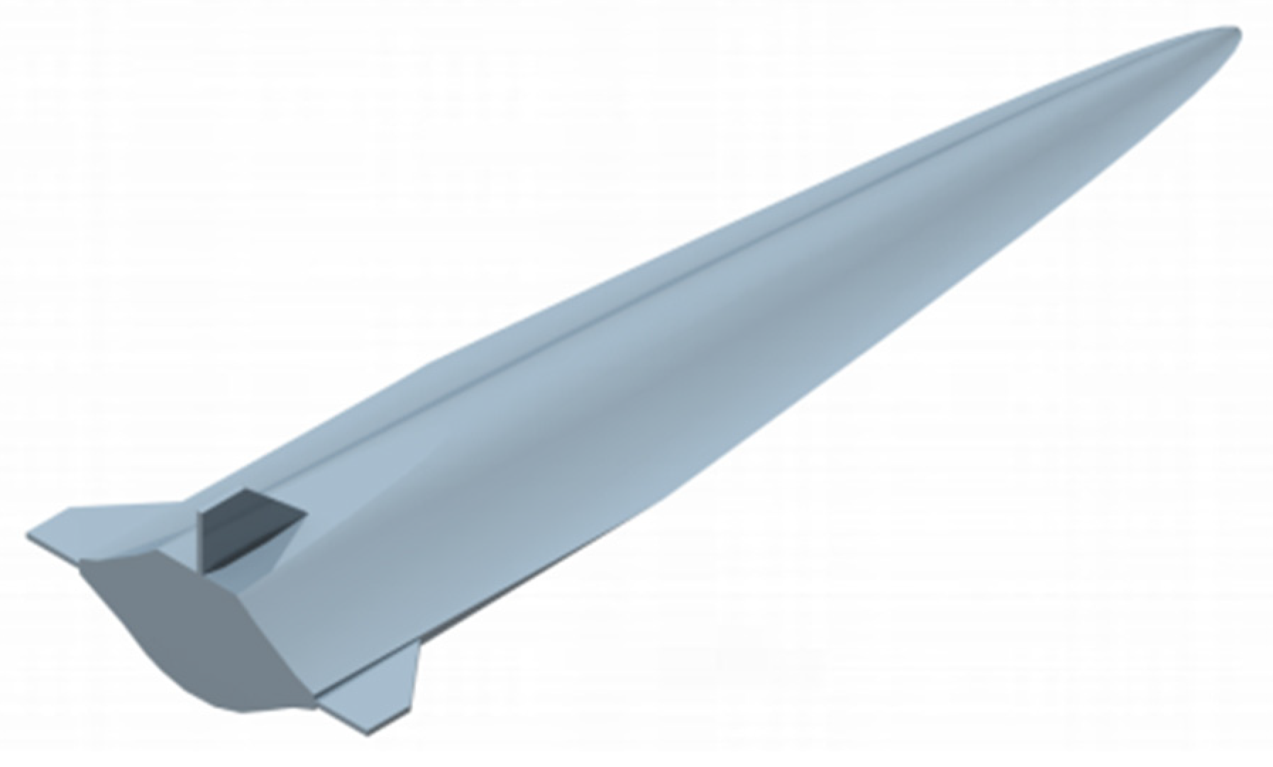
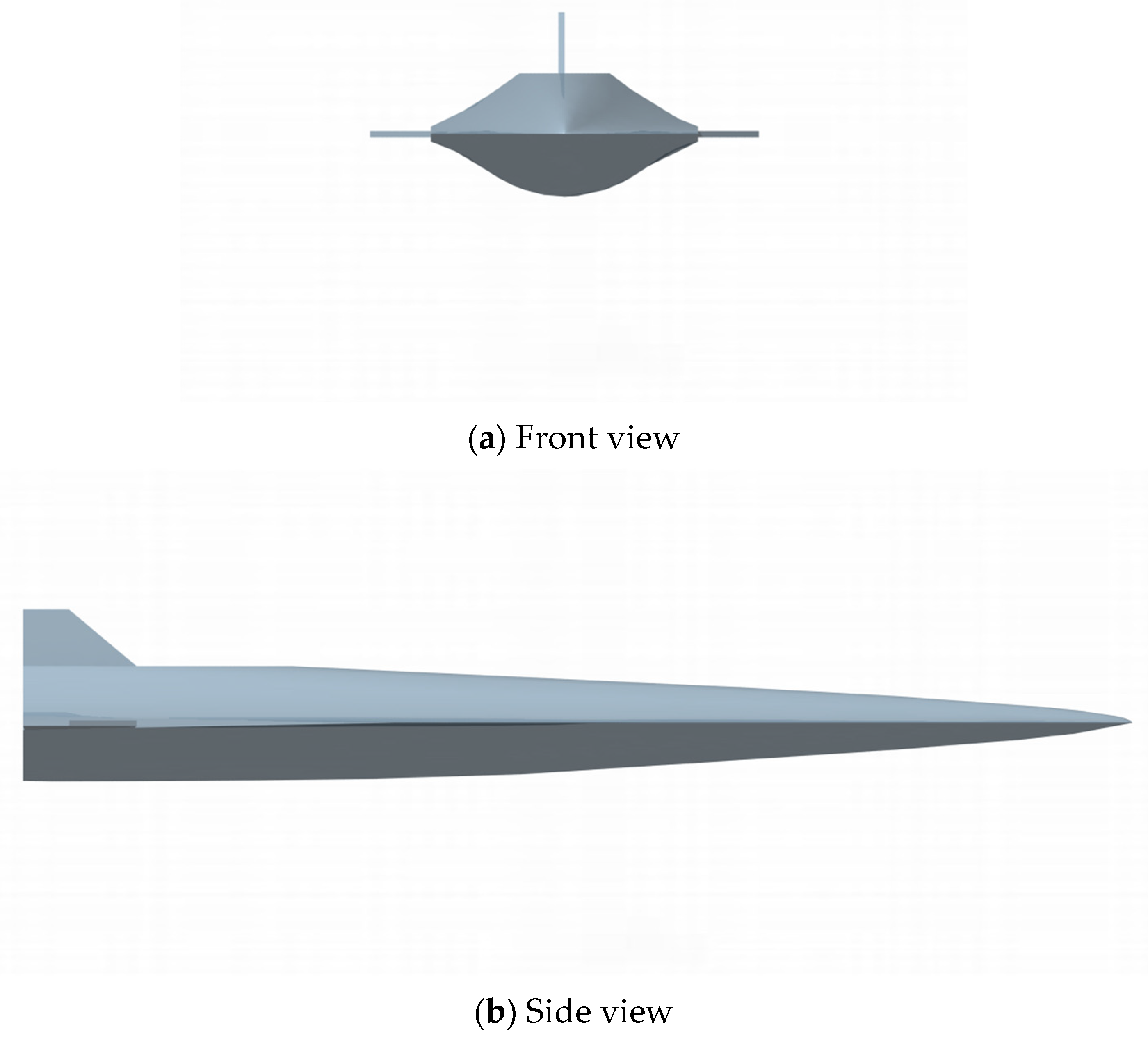
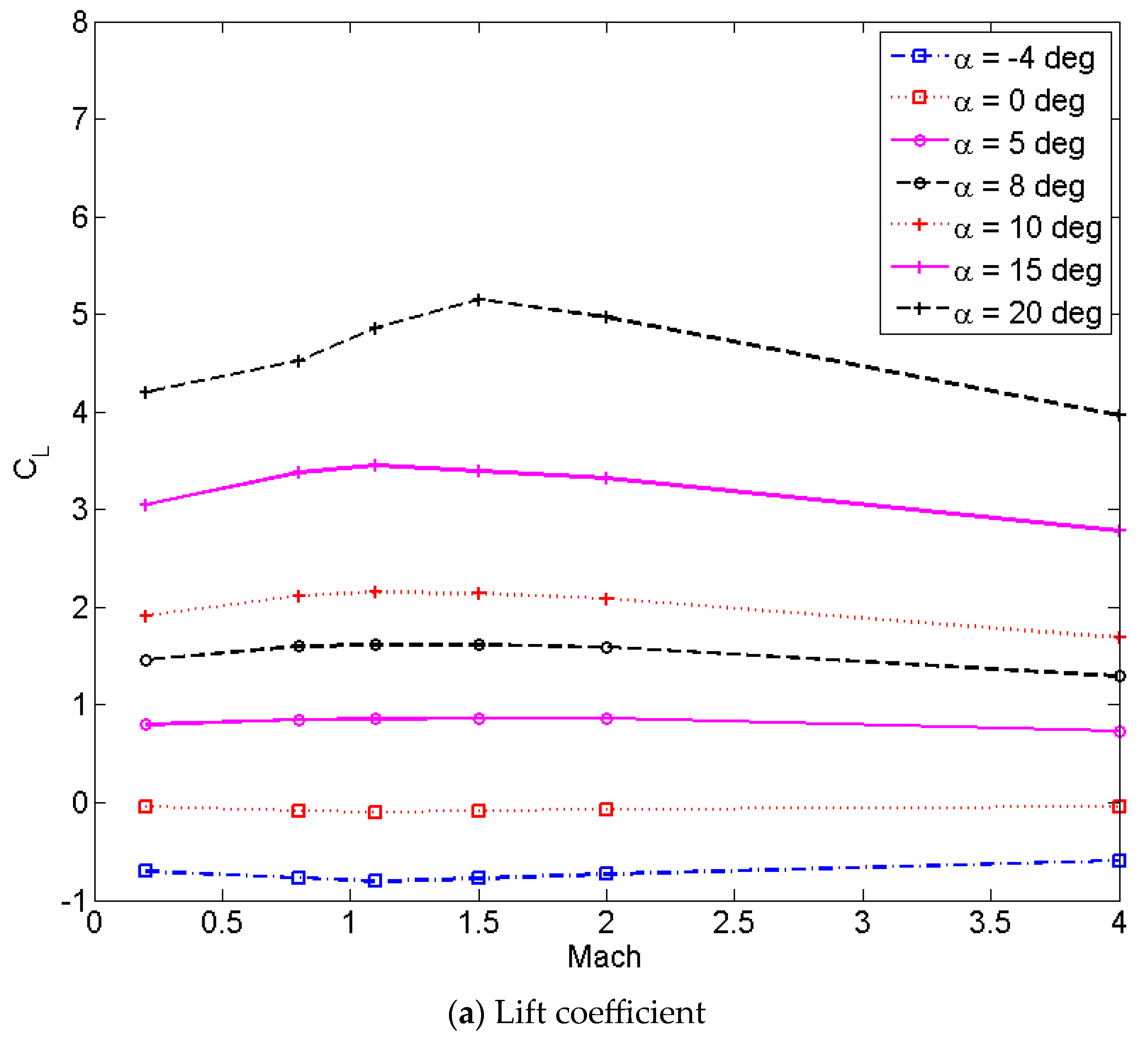
2.1. Wave-Rider Aircraft Aerodynamics and Modeling
2.2. The Longitudinal Dynamic Equations in the Energy Domain
2.3. Equation Constraints
2.4. Path Constraints
2.5. Optimization Objective Function
2.6. Trajectory Samples Design
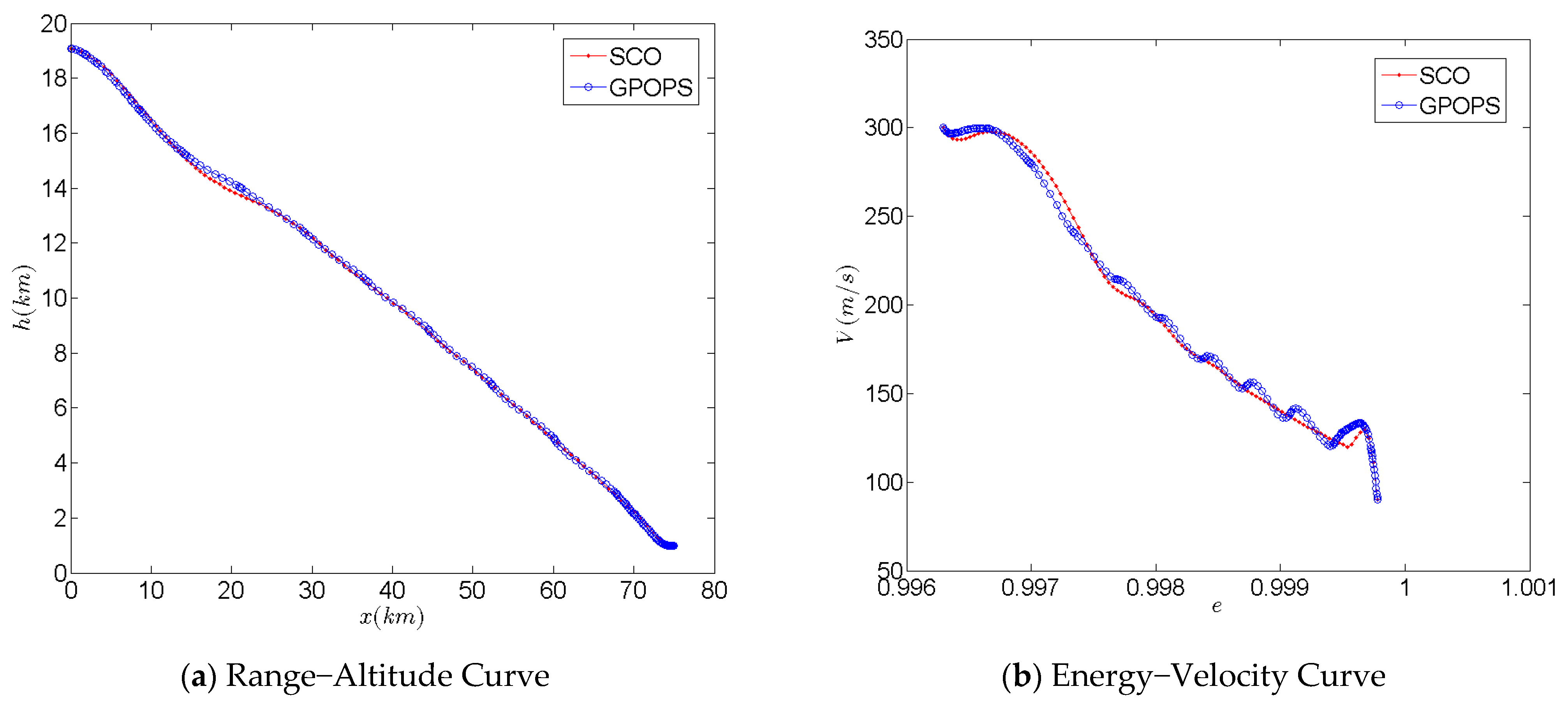
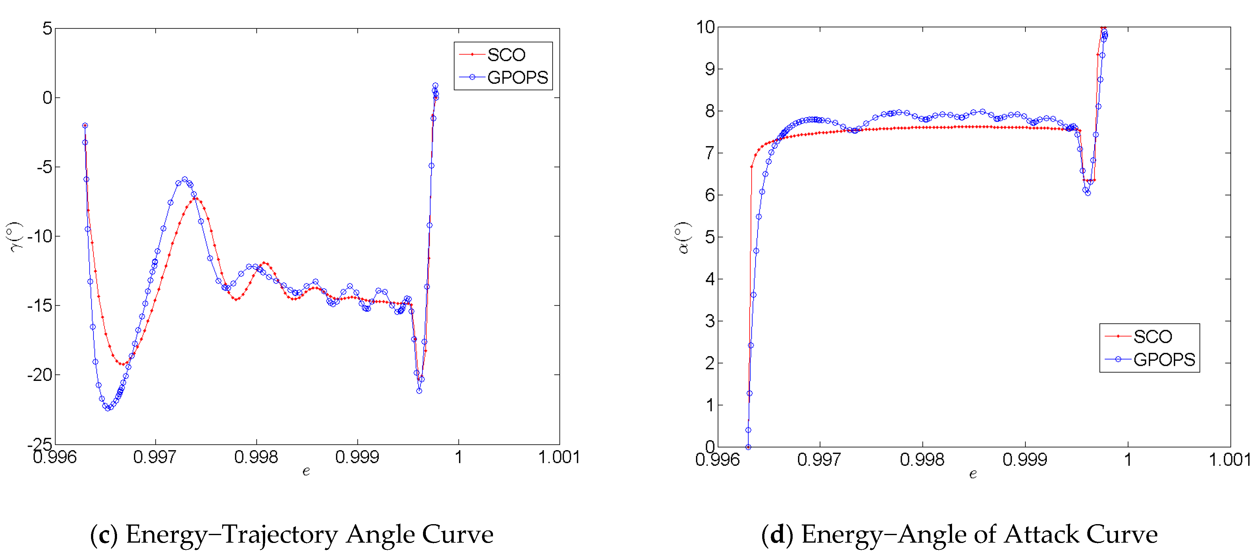
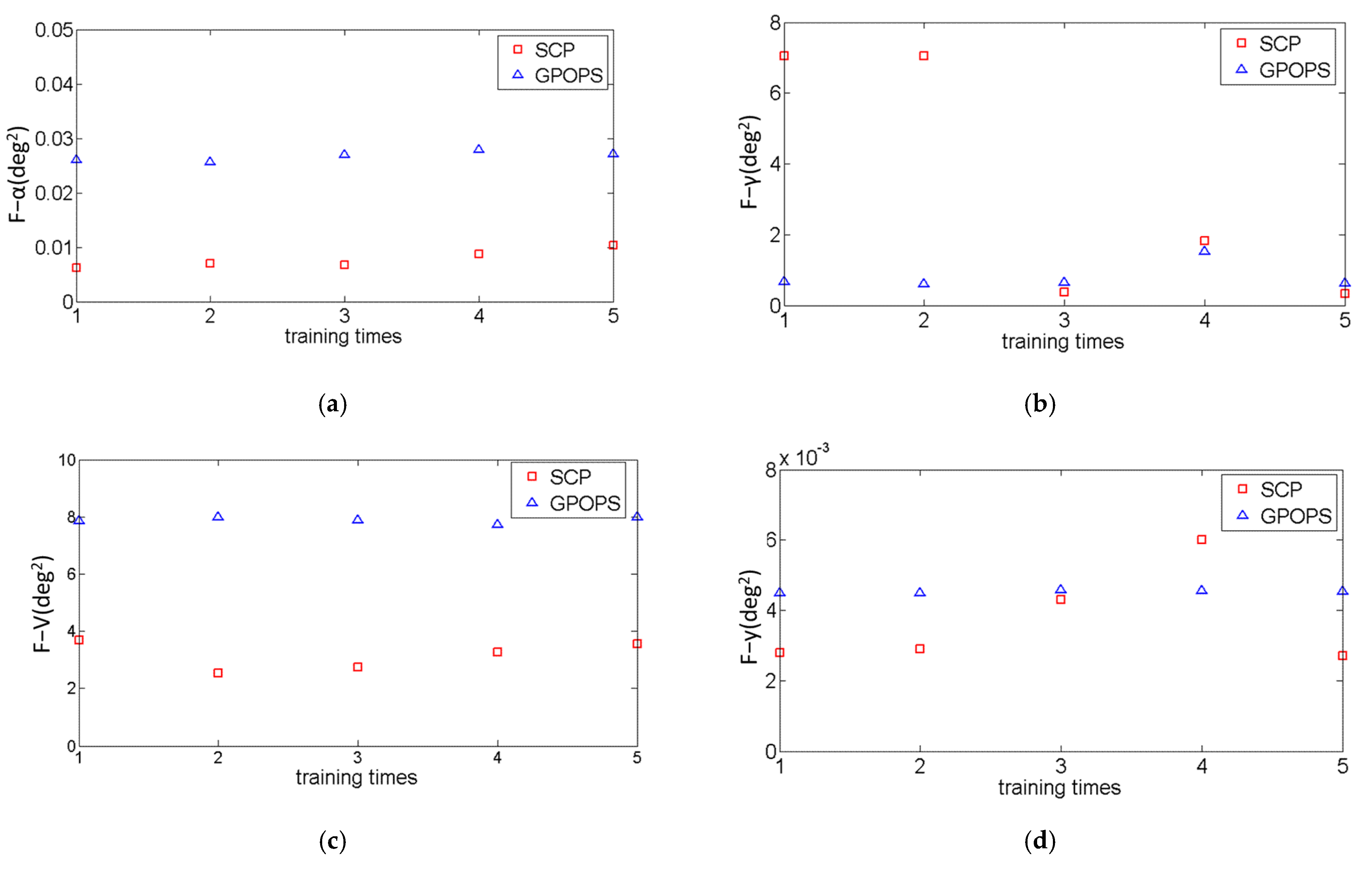
2.7. Accuracy and Convergence Analysis of the Optimization Method
2.8. Convergence Analysis
3. The Nonlinear Programming (NLP) Method
4. Building and Training Deep Neural Networks
5. Online Trajectory Generation
6. Summary
Author Contributions
Funding
Data Availability Statement
Conflicts of Interest
References
- Shen, H.-L.; Gong, Z. Methodology of Onboard Trajectory Design for Space Shuttle Terminal Area Energy Management Phase. J. Astronaut. 2008, 29, 430–433. [Google Scholar]
- Zhao, Z.-T.; Huang, W.; Yan, L.; Yang, Y.-G. An overview of research on widespeed range waverider configuration. Prog. Aerosp. Sci. 2020, 113, 100606. [Google Scholar] [CrossRef]
- Corraro, F.; Morani, G.; Nebula, F.; Cuciniello, G.; Palumbo, R. GN&C Technology Innovations for TAEM USV DTFT2 Mission Results. In Proceedings of the 17th AIAA International Space Planes and Hypersonic Systems and Technologies Conference, San Francisco, CA, USA, 11–14 April 2011. [Google Scholar]
- Corraro, F.; Cuciniello, G.; Morani, G.; Nebula, F.; Palumbo, R.; Vitale, A. Advanced GN&C Technologies for TAEM: Flight Test Results of the Italian Unmanned Space Vehicle. In Proceedings of the AIAA Guidance, Navigation, and Control Conference, Portland, OR, USA, 8–11 August 2011. [Google Scholar]
- Moore, T.E. Space Shuttle Entry Terminal Area Energy Management; NASA Johnson Space Center: Houston, TX, USA, 1991.
- Sun, C.Z. Research on Terminal Area Energy Management and Autolanding Technology for Reusable Launch Vehicle. Ph.D. Thesis, Nanjing University of Aeronautics and Astronautics, Nanjing, China, January 2008. [Google Scholar]
- Fang, G.C. Guidance Law Design of Terminal Area Energy Management for Reusable Launch Vehicle. Master Thesis, Nanjing University of Aeronautics and Astronautics, Nanjing, China, January 2013. [Google Scholar]
- Guo, T.; Xie, L. Research on Ship Trajectory Classification Based on a Deep Convolutional Neural Network. J. Mar. Sci. Eng. 2022, 10, 568. [Google Scholar] [CrossRef]
- Wang, J.; Wu, Y.; Liu, M.; Yang, M.; Liang, H. A Real-Time Trajectory Optimization Method for Hypersonic Vehicles Based on a Deep Neural Network. Aerospace 2022, 9, 188. [Google Scholar] [CrossRef]
- Hart, S.T.; Ayoubi, M.A.; Naseradinmousavi, P. Comparative Study of Pseudospectral Methods for Spacecraft Optimal Attitude Maneuvers. J. Spacecr. Rocket. 2022, 59, 178–189. [Google Scholar] [CrossRef]
- Haiping, R.A.O.; Zhong, R.; Pengjie, L.I. Fuel-optimal deorbit scheme of space debris using tethered space-tug based on pseudospectral method. Chin. J. Aeronaut. 2021, 34, 210–223. [Google Scholar]
- Zong, Q.; Li, Z.Y.; Ye, L.Q.; Tian, B. Variable trust region sequential convex programming for RLV online reentry trajectory reconstruction. J. Harbin Inst. Technol. 2020, 52, 147–155. [Google Scholar]
- An, K.; Guo, Z.-Y.; Xu, X.-P.; Huang, W. A framework of trajectory design and optimization for the hypersonic gliding vehicle. Aerosp. Sci. Technol. 2020, 106, 106110. [Google Scholar] [CrossRef]
- Liu, Z.; Lu, H.R.; Zheng, W.; Wen, G.; Wang, Y.; Zhou, X. Rapid time-coordination trajectory planning method for multi-glide vehicles. Acta Aeronaut. Astronaut. Sin. 2021, 42, 524479. [Google Scholar]
- Wei, J.-H.; Wang, Z.-K. Glide-Cruise Trajectory Optimization for Hypersonic Vehicles. J. Command. Control. 2021, 7, 249–256. [Google Scholar]
- Li, Z.; Zhou, X.; Zhang, H.; Tang, G. Analysis of Entry Footprint Based on Pseudospectral Method. J. Shanghai Jiao Tong Univ. 2022, 56, 1470–1478. [Google Scholar]
- Ren, P.F.; Wang, H.B.; Zhou, G.F. Reentry trajectory optimization for hypersonic vehicle based on adaptive pseudospectral method. J. Beijing Univ. Aeronaut. Astronaut. 2019, 45, 2257–2265. [Google Scholar]
- Boyd, S.; Vandenberghe, L. Convex Optimization; Cambridge University Press: Cambridge, UK, 2004. [Google Scholar]
- Wang, B. Implementation of Interior Point Methods for Second Order Conic Optimization. Ph.D. Thesis, McMaster University, Hamilton, ON, Canada, 2003. [Google Scholar]
- Andersen, E.D.; Roos, C.; Terlaky, T. On implementing a primal-dual interior-point method for conic quadratic optimization. Math. Program. 2003, 95, 249–277. [Google Scholar] [CrossRef]
- Andersen, E.D.; Andersen, K.D. The MOSEK Interior Point Optimizer for Linear Programming: An Implementation of the Homogeneous Algorithm; High Performance Optimization; Springer US: New York, NY, USA, 1996; pp. 197–232. [Google Scholar]
- Vandenberghe, L. The CVXOPT Linear and Quadratic Cone Program Solvers. 20 March 2010. Available online: http://www.seas.ucla.edu/~vandenbe/publications/coneprog.pdf (accessed on 3 January 2023).
- Domahidi, A.; Chu, E.; Boyd, S. ECOS: An SOCP Solver for Embedded Systems. In Proceedings of the 2013 European Control Conference (ECC), Zürich, Switzerland, 17–19 July 2013. [Google Scholar]
- Domahidi, A. Methods and Tools for Embedded Optimization and Control. Ph.D. Thesis, RWTH Aachen University, Aachen, Germany, 2013. [Google Scholar]
- Liu, X.; Shen, Z.; Lu, P. Entry Trajectory Optimization by Second-Order Cone Programming. J. Guid. Control. Dyn. 2015, 39, 227–241. [Google Scholar] [CrossRef]
- Liu, X.; Shen, Z.; Lu, P. Exact convex relaxation for optimal flight of aerodynamically controlled missiles. IEEE Trans. Aerosp. Electron. Syst. 2016, 52, 1881–1892. [Google Scholar] [CrossRef]
- Mao, Y.; Szmuk, M.; Açıkmeşe, B. Successive Convexification of Non-Convex Optimal Control Problems and Its Convergence Properties. In Proceedings of the 2016 IEEE 55th Conference on Decision and Control (CDC), Las Vegas, NV, USA, 12–14 December 2016. [Google Scholar]
- Liu, X.; Lu, P.; Pan, B. Survey of convex optimization for aerospace applications. Astrodynamics 2017, 1, 23–40. [Google Scholar] [CrossRef]
- Szmuk, M.; Açıkmeşe, B. Successive Convexification for 6-DoF Mars Rocket Powered Landing with Free-Final-Time. In Proceedings of the 2018 AIAA Guidance, Navigation, and Control Conference, Kissimmee, FL, USA, 8–12 January 2018. [Google Scholar]
- Mao, Y.; Szmuk, M.; Açıkmeşe, B. Successive Convexification: A Superlinearly Convergent Algorithm for Non-convex Optimal Control Problems. arXiv 2018, arXiv:1804.06539. [Google Scholar]
- Szmuk, M.; Reynolds, T.P.; Açıkmeşe, B. Successive Convexification for Real-Time 6-Dof Powered Descent Guidance with State-Triggered Contraints. arXiv 2018, arXiv:1811.10803. [Google Scholar]
- Liu, X. Fuel-Optimal Rocket Landing with Aerodynamic Controls. In Proceedings of the AIAA Guidance, Navigation, and Control Conference, Grapevine, TX, USA, 9–13 January 2017. [Google Scholar]
- Reynolds, T.P.; Szmuk, M.; Malyuta, D.; Mesbahi, M.; Açıkmeşe, B. Dual Quaternion Based Powered Descent Guidance with State-Triggered Constraints. J. Guid. Control. Dyn. 2019, 43, 1584–1599. [Google Scholar] [CrossRef]
- Wang, Z.; Grant, M.J. Improved Sequential Convex Programming Algorithms for Entry Trajectory Optimization. In Proceedings of the AIAA SciTech Forum, San Diego, CA, USA, 7–11 January 2019. [Google Scholar]
- Han, H.; Qiao, D.; Chen, H.; Li, X. Rapid planning for aerocapture trajectory via convex optimization. Aerosp. Sci. Technol. 2019, 84, 763–775. [Google Scholar] [CrossRef]
- Pei, P.; Wang, J. Near-Optimal Guidance with Impact Angle and Velocity Constraints Using Sequential Convex Programming. Math. Probl. Eng. 2019, 2019, 2065730. [Google Scholar] [CrossRef]
- Malyuta, D.; Reynolds, T.P.; Szmuk, M.; Açıkmeşe, B. Fast Trajectory Optimization via Successive Convexification for Spacecraft Rendezvous with Integer Constraints. arXiv 2019, arXiv:1906.04857. [Google Scholar]
- Chen, B.; Liu, C.; Ji, C. Waverider design and analysis based on shock-fitting method. ACTA Aerodyn. Sin. 2017, 35, 421–428. [Google Scholar]
- Liu, C.; Bai, P.; Chen, B.; Ji, C. Rapid Design and Multi-Object Optimization for Waverider from 3D Flow. J. Astronaut. 2016, 29, 535–543. [Google Scholar]
- Li, D.; Ji, C.; Ma, H. Three dimensions unstructured Cartesian grid for Navier-Stokes equation. ACTA Aerodyn. Sin. 2006, 24, 6. [Google Scholar]


| Initial Conditions | e0 | γ0 (°) | V0 (m/s) | |
|---|---|---|---|---|
| Value | 0.996297 | 0, −1, −2, −3, −4, −5 | 280, 290, 300, 325, 350, 370 | |
| Terminal conditions | yf (km) | γf (°) | Vf (m/s) | xf (km) |
| Value | 1.0 | 0.0 | 90.0 | [35,36,…,73] |
| xf (km) | SCO (s) | GPOPS (s) |
|---|---|---|
| 35 | 40.6 | 108.5 |
| 55 | 25.5 | 135.7 |
| 75 | 41.7 | 90.2 |
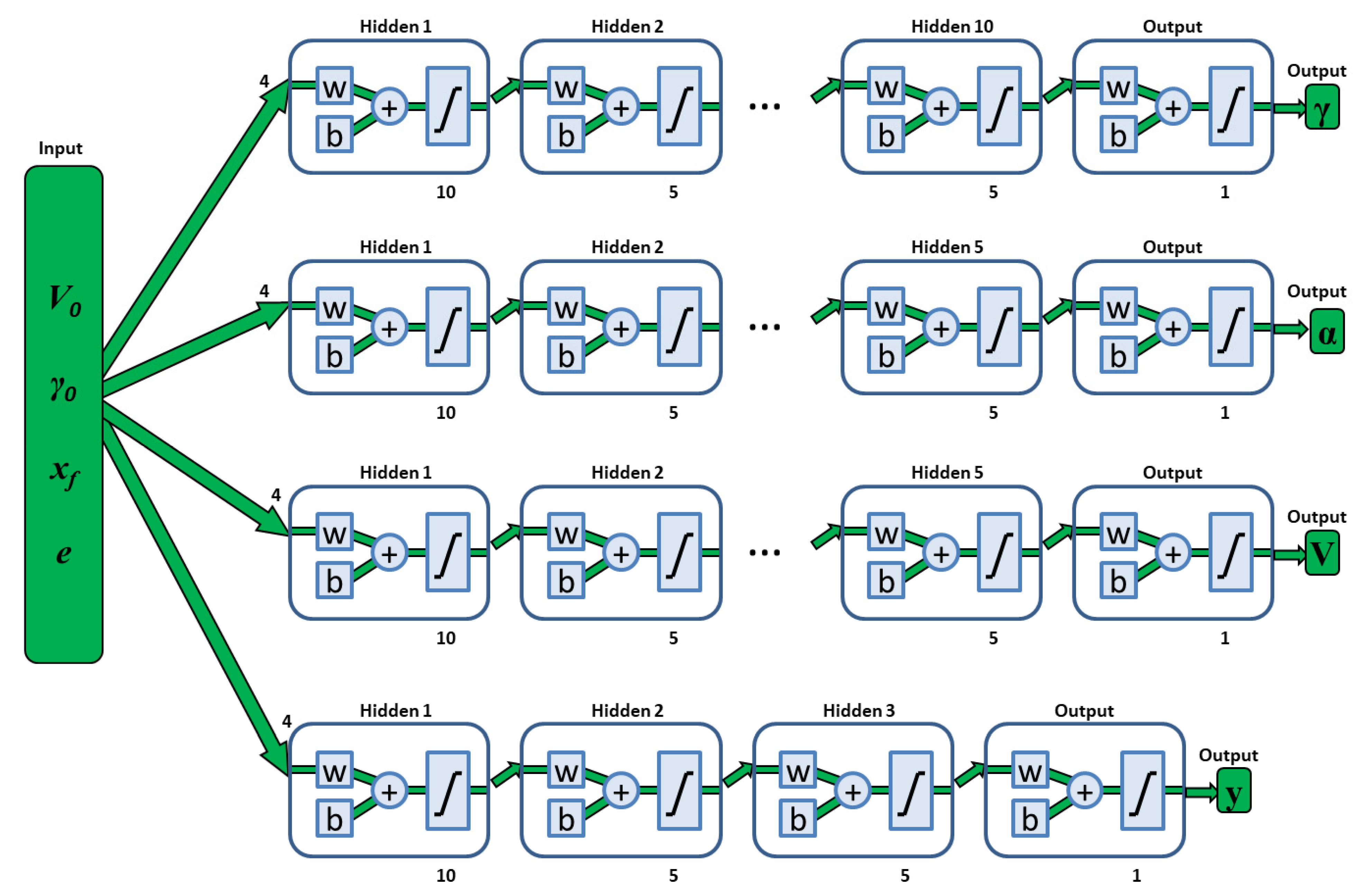
| Networks | Flight Path Angle Network | Angle of Attack Network | Velocity Network | Altitude Network |
|---|---|---|---|---|
| Inputs | V0,γ0,xf, e | V0,γ0,xf, e | V0,γ0,xf, e | V0,γ0,xf, e |
| Outputs | γ | α | V | y |
| Number of Hidden Layers | 10 | 5 | 5 | 3 |
| Number of Neurons per Hidden Layer | [10,5,5,…,5] | [10,5,5,5,5] | [10,5,5,5,5] | [10,5,5] |
| Activation Function | tansig | tansig | tansig | tansig |
| Number of Weights | 306 | 201 | 201 | 141 |
| Training Method | Levenberg–Marquardt | Levenberg–Marquardt | Levenberg–Marquardt | Levenberg–Marquardt |
Disclaimer/Publisher’s Note: The statements, opinions and data contained in all publications are solely those of the individual author(s) and contributor(s) and not of MDPI and/or the editor(s). MDPI and/or the editor(s) disclaim responsibility for any injury to people or property resulting from any ideas, methods, instructions or products referred to in the content. |
© 2023 by the authors. Licensee MDPI, Basel, Switzerland. This article is an open access article distributed under the terms and conditions of the Creative Commons Attribution (CC BY) license (https://creativecommons.org/licenses/by/4.0/).
Share and Cite
Liu, Z.; Yan, J.; Ai, B.; Fan, Y.; Luo, K.; Cai, G.; Qin, J. An Online Generation Method of Terminal-Area Trajectories for Wave-Rider Using Deep Neural Networks. Aerospace 2023, 10, 654. https://doi.org/10.3390/aerospace10070654
Liu Z, Yan J, Ai B, Fan Y, Luo K, Cai G, Qin J. An Online Generation Method of Terminal-Area Trajectories for Wave-Rider Using Deep Neural Networks. Aerospace. 2023; 10(7):654. https://doi.org/10.3390/aerospace10070654
Chicago/Turabian StyleLiu, Zhe, Jie Yan, Bangcheng Ai, Yonghua Fan, Kai Luo, Guodong Cai, and Jiankai Qin. 2023. "An Online Generation Method of Terminal-Area Trajectories for Wave-Rider Using Deep Neural Networks" Aerospace 10, no. 7: 654. https://doi.org/10.3390/aerospace10070654
APA StyleLiu, Z., Yan, J., Ai, B., Fan, Y., Luo, K., Cai, G., & Qin, J. (2023). An Online Generation Method of Terminal-Area Trajectories for Wave-Rider Using Deep Neural Networks. Aerospace, 10(7), 654. https://doi.org/10.3390/aerospace10070654