Article

Physics-Guided Neural Network Model for Aeroengine Control System Sensor Fault Diagnosis under Dynamic Conditions

School of Power and Energy, Northwestern Polytechnical University, Xi’an 710072, China
*
Author to whom correspondence should be addressed.
Aerospace 2023, 10(7), 644; https://doi.org/10.3390/aerospace10070644
Submission received: 30 May 2023 / Revised: 13 July 2023 / Accepted: 14 July 2023 / Published: 18 July 2023
(This article belongs to the Special Issue Aerospace Prognosis Technology)

Abstract

:
Sensor health assessments are of great importance for accurately understanding the health of an aeroengine, supporting maintenance decisions, and ensuring flight safety. This study proposes an intelligent framework based on a physically guided neural network (PGNN) and convolutional neural network (CNN) to diagnose sensor faults under dynamic conditions. The strength of the approach is that it integrates information from physics-based performance models and deep learning models. In addition, it has the structure of prediction–residual–generation-fault classification that effectively decouples the interaction between sensor faults and system state changes. First, a PGNN generates the engine’s non-linear dynamic prediction output because the PGNN has the advantage of being able to handle temporal information from the long short-term memory (LSTM) network. We use a cross-physics–data fusion scheme as the prediction strategy to explore the hidden information of the physical model output and sensor measurement data. A novel loss function that considers physical discipline is also proposed to overcome the performance limitations of traditional data-driven models because of their physically inconsistent representations. Then, the predicted values of the PGNN are compared with the sensor measurements to obtain a residual signal. Finally, a convolutional neural network (CNN) is used to classify faults for residual signals and deliver diagnostic results. Furthermore, the feasibility of the proposed framework is demonstrated on an engine sensor fault dataset. The experimental results show that the proposed method outperforms the pure data-driven approach, with the predicted RMSE being reduced from 1.6731 to 0.9897 and the diagnostic accuracy reaching 95.9048%, thereby confirming its superior performance.

1. Introduction

As technology evolves, aeroengine control systems become increasingly complex [1,2,3]. The variable engine operating conditions and harsh operating conditions increase the system’s vulnerability, leading to unpredictable sensor faults during the aeroengine’s operation. Reliable and efficient diagnostic and health-monitoring systems can reduce maintenance costs, extend service life, and ensure aeroengine safety [4,5,6].
Aeroengines involve the integration of multidisciplinary technologies with a sophisticated structure. In contrast to other industrial equipment, aeroengines have a wide flight envelope and their operating conditions are often in transition [7]. For example, when the pilot pushes the throttle lever, the engine rotations increase from about 6000 rpm to 13,000 rpm. As the rotor speed increases, the various engine cross-section parameters also change. The features of the sensor measurement have a significant correlation with the engine operating conditions. The neural network may judge a change in these engine operating conditions to be a fault. To expand the applicability of the fault diagnosis method and correctly diagnose the fault of the engine control system sensors, even under dynamic conditions, the fault diagnosis method must be improved.
The main technologies for aeroengine fault diagnosis are model-based, signal-based, and data-driven methods. Model-based methods analyze the dynamic characteristics of an engine on the basis of physical principles, such as Kalman filters (KFs) [8,9], unknown input observers (UIOs) [10], and sliding mode observers (SMOs) [11]. The advantages of this method are its high interpretability and fast diagnosis. As long as the accurate engine model is known, it is possible to calculate and estimate the needed information. However, physics-based models are complex and incomplete due to their complex modeling engines.
The signal-based approach does not require an accurate model of the object [12]. It usually uses the system output signal to detect faults by directly analyzing the measurable signal through various signal-processing techniques, such as wavelet analyses [13] and empirical modal decomposition [14]. This method is highly adaptable, but its disadvantage is that it can only detect faults with relatively obvious mutation characteristics [15].
The increase in system condition-monitoring data has facilitated the widespread use of data-driven approaches for engine health management. The underlying assumption of data-driven approaches is that the relevant information about the evolution of system fault times can be learned from past data [16,17,18]. In particular, deep learning (DL) has recently gained attention [19,20,21]. DL models mine data from large amounts of training data with multiple non-linear layer hierarchies through greedy layer-by-layer pre-training, backward fine-tuning, and various non-linear activation functions. Their diagnostic results are dramatically improved compared to those of traditional intelligence methods. Some popular DL models are deep neural networks (DNNs) [22], auto-encoders (AEs) [23], convolutional neural networks (CNNs) [24], deep belief networks (DBNs) [25], and recurrent neural networks (RNNs) [26]. Traditional DL models are considered to be complex black-box models [27,28,29], and the model’s output does not necessarily follow the laws of physics to produce physically consistent results [30].
Although data-driven and physics-based approaches have their limitations when applied in isolation, it is hypothesized here that the combined use of the two approaches has the potential to improve their performances, as the strengths of both can be exploited. This has led to increased research on how to improve DL models by incorporating prior knowledge into the learning process. This is one of the ways in which the black-box nature of the model can be improved. A potential solution is the integration of prior knowledge into the training process, which leads to the concept of informed machine learning [30]. For example, logic rules [31,32] or algebraic equations [33,34] have been added as constraints to loss functions. Scholars refer to these as physics-informed neural networks (PINNs) [33], physics-guided neural networks (PGNNs) [35], and physics-aware neural networks (PANNs) [36].
Compared to a purely data-driven network model, the information flow of a PGNN includes prior knowledge in addition to training data. In a PGNN, the principles of physics are used to inform the search for a physically meaningful and accurate DL model. Hybrid systems combining thermodynamic performance models and data-driven aging models have shown promising results on simpler systems (e.g., lithium batteries) [37]. Arka Daw created a PGNN model to predict lake water temperature at different depths and times and verified the effectiveness of the PGNN [35]. Wang integrated a new physics-guided GRU model (PGGM) with data-driven models and physical knowledge for predicting tool wear and verified that the model without a physical mapper did not perform as well as the PGGM [29]. Manuel-fused physics and deep-learning-based prediction models for predicting the remaining life of engines and experimental results showed that the hybrid framework outperformed a purely data-driven approach, extending the prediction range by nearly 127% [38].
Both model-based and data-driven approaches have been well studied in aeroengine sensor fault diagnosis [4,39]. Sun [9] proposed and implemented the hyperelliptic Kalman filter for aeroengine sensor fault isolation and accommodation. Du [40] proposed the Inception-CNN to predict the probability of aeroengine sensor failures. The above two fault diagnosis methods will eventually be integrated through information fusion techniques, in addition to developing alone in their respective technical fields [39,41]. Huang [42] used a KF bank for the fault diagnosis of aeroengine sensors. Extreme learning machine (ELM) models are trained to modify the on-board model and KF outputs, greatly improving the accuracy of the model. But this approach is only a combination of model and data methods. It is possible for a PGNN to embed model information into a DL model. However, there is little published work on the application of PGNNs for diagnosing faults in aeroengine control system sensors. For this purpose, a new intelligent diagnostic method is proposed for the sensor fault diagnosis of aeroengine control systems under dynamic conditions. The approach blends engine model knowledge with deep learning algorithms, while overcoming some of their limitations. The underlying assumption of this approach is that the output of the physics-based model is as much related to the engine running process as it is to time. This is the first attempt to use a PGNN for fault diagnosis in engine control system sensors.
Overall, the main contributions of this paper are threefold.
(1)
A PGNN–CNN-based intelligent diagnosis method is provided to solve the fault diagnosis problem of aeroengine control system sensors under dynamic conditions. Firstly, a PGN generates sensor predictions, which are synthesized with the sensor measurements to generate residuals, and then a powerful classification model, the CNN, is used to provide diagnostic results. Through the structure of the prediction–residual–fault classification, the effect of changing the engine flight conditions on the measured engine output is attenuated through residual generation.
(2)
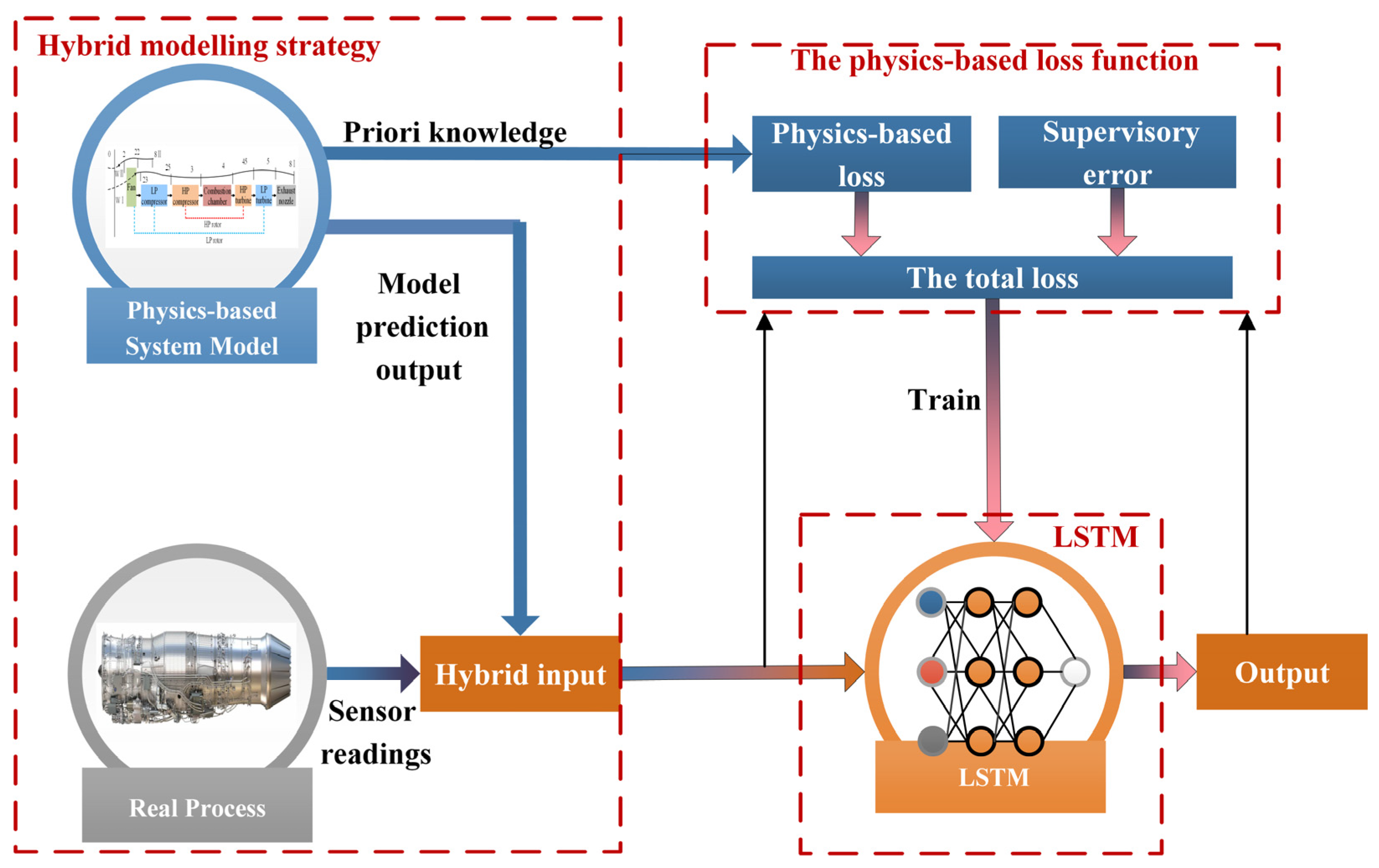
A sensor prediction strategy based on a hybrid physics–data model is proposed. By merging the physics-based model and data-driven model for the prediction, data mining and physics principles are effectively combined. The PGNN model fully explores the implicit relationship between the input and output and improves the prediction accuracy.
(3)
A new loss function, the physics-guided loss function, is suggested. The physically guided loss function considers physical knowledge by mapping monitoring data and time to a potential variable associated with engine dynamics. Physical inconsistencies in parameters and prediction results are eliminated, thus improving the performance of the PGNN.
The rest of the paper is organized as follows: Section 2 describes the physically guided data-driven model and the methodology used for the data-driven model. Section 3 details the architecture and the fault diagnosis scheme. Section 4 provides the validation results of the experimental data, experimental analysis, and experimental results. Finally, the conclusions are stated in Section 5.

2. Physically Guided Neural Network Model

Most DL algorithms are implemented as black-box functions, where the extraction of abstract relations in the data is left to the machine. In this respect, attempts have been made to explain and constrain these techniques from a physics perspective. A new paradigm is offered to explore further information or experiences in big data while considering theoretical knowledge. This paradigm for integrating scientific knowledge and data science is known as theory-guided data science [29]. It is also called a physically guided neural network or a physically informed data-driven model. In contrast to traditional data-driven models, a PGNN eliminates physical inconsistencies that conflict with empirical knowledge or physical disciplines. Physical knowledge is cleverly integrated into the data-driven model based on the PGNN’s scheme, thus overcoming the disadvantages of pure data and purely physical models.
Building a PGNN involves three key steps [29,37]: (1) creating a hybrid combination of physics-based model knowledge and a neural network, i.e., a hybrid physics-based data model; (2) using scientific knowledge as a physics-based loss function in the learning objective of the neural network; and (3) training the model. The specific steps are shown below.
Consider a learning or classification problem with a set of inputs X physically linked to a target variable Y. The standard approach is to train a data-driven model, such as a neural network f N N : X Y , on a set of data instances, which can then estimate the target variable Y. The data-driven model essentially approximates a function that, by providing data points, adjusts the parameters of the neural network to achieve a good fit. For a given data point, the neural network interpolates in a model agnostic, and therefore non-physical, manner.
Alternatively, a physically based mathematical model f P H Y : X Y can be developed to simulate the values of the target variables Y P H Y . Due to the complexity of engine models, the physically based model f P H Y is often influenced by model simplifications and noise, etc. Y P H Y may provide an incomplete representation of the target variables, resulting in discrepancies between the model and the observed data. The hybrid physics–data model aims to exploit the physical information and the data, bringing them together to overcome their shortcomings.
A general neural network has a loss function of the form.
L o s s = 1 n i = 1 n ( Y i Y ^ i ) 2
Here, Y ^ is the neural network’s predicted output and the actual measured value.
The physical constraint term can act as a norm regularization term, which serves as a penalty constraint to limit the parameters in the loss function. Figure 1 displays a framework for a loss function strategy based on physical information. The blue box indicates the supervisory loss and depicts the difference between the predictions and observations. In a traditional data-driven model, a loss function is built based on this loss to optimize the model. In addition to the supervisory loss, the theoretically guided framework includes domain-knowledge-based loss (shown in the red box). Finally, a total loss function based on physical information is obtained using a linear combination of all the above penalty terms, expressed as follows:
L o s s = L ( Y , Y ^ ) + λ R p h y ( X , Y ^ )
Here, Y ^ represents the predicted output and Y stands for the target output. L is a traditional data-driven model’s loss function, which measures the supervisory error between the target and predicted outputs. R p h y is a physical regularization term based on Y ^ , and the physical principle equations quantify the constraints of a given prior knowledge equation and aim to ensure consistency with the laws of physics. λ represents the hyperparameters, which determine the weight of the physical regularization terms.
It is assumed that the following equation can express the physical relationship between the physical variables in the study problem:
G ( X , Y ) = 0 H ( X , Y ) 0
G and H represent general forms of physically based equations, such as thermodynamic equations and control equations. These physics-based equations must satisfy the same criteria as the other loss function terms (i.e., continuous and differentiable). The physics-based loss function may be of the following form:
R p h y = G ( X , Y ^ ) 2 + ReLU ( H ( X , Y ^ ) )
By assuming that the known laws of physics apply equally to any data instance, the loss function uses prior physical knowledge as a source of information to guarantee the generalization ability of the PGNN model, ensuring that models with physical consistency are used as learning targets for a PGNN. The neural network model weights will be searched within the constraints consistent with the physical knowledge. The prior physical knowledge eliminates physical inconsistencies hidden in the model parameters and target results without affecting their bias [26].
How to relate the systems with complex engine dynamics to the condition-monitoring sensor readings and embed them in the training of neural networks is an important issue in aeroengine control system sensor fault diagnosis. Therefore, the following section proposes details of the PGNN model used for this task.

3. The Proposed Method

To ensure an accurate fault diagnosis and estimation of the sensor signals under dynamic conditions, a PGNN–CNN-based intelligent method is proposed to facilitate a tight integration between data-driven learning and the physics-based model. The structure of the method is shown in Figure 2. The general procedure is as follows:
(1)
Data acquisition: The sensor data of the aeroengine control system under dynamic conditions are collected. Then, the data are labeled and the labeled dataset is segmented and grouped into two categories: a training set and a test set.
(2)
Data standardization: The signal is normalized and rescaled to the range [0, 1].
(3)
Physics-based aeroengine model: Physics-based aeroengine models are built to obtain physics-guided prediction outputs.
(4)
PGNN-based prediction: The engine input data and the prediction output of the physics-based aeroengine model engine are sent to the PGNN to obtain the predicted output of the engine.
(5)
Residual generation: The actual sensor output of the engine control system is subtracted from the predicted outcome of the PGNN to obtain the residual.
(6)
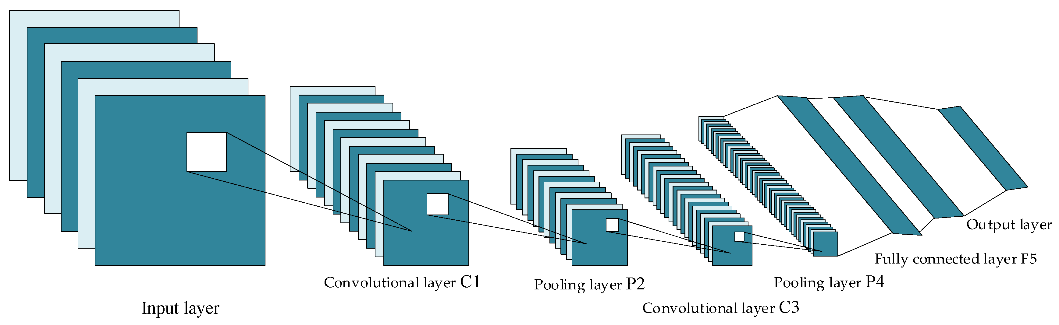
CNN-based fault classification: The residual vector is fed to the CNN-based model to automatically obtain the final diagnosis result.
(7)
Model evaluation: The trained model is evaluated to obtain a PGNN–CNN model with a satisfactory performance.
Figure 2. Flow chart of the proposed method.
Aerospace 10 00644 g002
The details of the method proposed in this paper are discussed below.

3.1. Data Standardization

In practice, the units of measurement for different variables are often inconsistent [43]. The data are often standardized before analysis to eliminate the dimensional effect of the variables and ensure that each variable has the same expressive power. As shown in Equation (5), the normalization of the measurement signals can make the mean value of the data approach 0 and the variance approach 1, reducing errors in the signal acquisition process, while reducing the computational complexity and computation time.
y k = x k x ¯ k σ ( x k )
where x ¯ k stands for the mean value of x k and σ ( x k ) represents the standard deviation of x k .

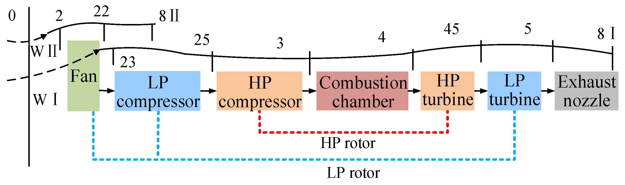
3.2. Physics-Based Aeroengine Model

Physics-based models of engine control systems can be used in the control and performance evaluations of aeroengines. These models can predict measured process variables (e.g., engine temperature, pressure, or rotational speed) and global unmeasured system performance (e.g., efficiency and power). The engine performance model is mathematically represented as a coupled system of non-linear equations. The inputs to the model are the engine operating conditions w and model parameters θ , and the outputs of the model are estimates of the measurable physical properties x ^ s and unmeasurable properties x ^ v . Thus, the aeroengine performance model can be expressed as [ x ^ s , x ^ v ] = F ( w , θ ) .
An aeroengine is a strongly non-linear system, and because of the complex modeling constraints, the modeling of engines is different from that of most other non-linear devices. An aeroengine is difficult to describe using an explicit equation [44,45]. The current common modeling approach is to model the non-linear components of an aeroengine based on the thermodynamic properties of these components. An aeroengine is a complex aerodynamic and thermodynamic system consisting of components that perform various functions. Each component can be described mathematically as a function of associated inputs and outputs. There are certain relationships between the parameters of each component, such as the flow balance, pressure balance, and power balance. These equilibrium relationships form a series of non-linear differential equations, which can be solved to obtain the engine output based on the engine inputs.
Figure 3 presents a structural sketch of the simulation engine model, which. This engine model is built based on the component characteristics and input–output relationships between the components. The aeroengine model includes a fan, a compressor, a combustion chamber, a turbine, and an exhaust nozzle [46,47].
The engine can be represented by a linear state space equation. Specific modeling methods have been reported previously [2], and the equation can be described as follows:
{ x ˙ ( t ) = A x ( t ) + B u ( t ) y ( t ) = C x ( t ) + D u ( t )
where A , B , C , D are the system matrices with appropriate dimensions; x ( t ) is the state variable; u ( t ) is the control variable; and y ( t ) is the output variable.
The engine’s predicted output can be obtained using Equation (6), but the poor interference capability of the physics-based model will affect the accuracy of the model. Therefore, the PGNN-based prediction model is constructed using both the prediction output of the model and the engine data.

3.3. PGNN-Based Prediction

Figure 4 illustrates an overview of the PGNN for engine output prediction. It consists of three steps. First, the engine prediction output is obtained from the engine model built in Section 3.2. The model prediction output and the sensor readings of the engine input variables are used as the hybrid input. Second, the hybrid input obtains prediction results while mapping to the LSTM prediction space with temporal characteristics. Third, a new loss function based on physical information is proposed to train the long short-term memory (LSTM) neural network to eliminate physical inconsistencies, considering the dynamic characteristics of the engine.
The hybrid input strategy that mixes the model and sensor readings, the LSTM network model with time–series characteristics, and the novel loss function together form the PGNN model proposed in this paper. The PGNN improves the long short-term memory (LSTM) neural network by providing more information through input mixing and eliminating physical inconsistencies through a new loss function. These improvements include a hybrid modeling strategy for physical data and embedding a novel physics-based loss function, as shown in Figure 4. The modeling details are as follows.

3.3.1. Hybrid Input

A wealth of information is contained in the engine operating history data. Physics-based models use simulation software and physics knowledge to simulate physical processes, which are well understood conceptually by following scientific principles. The aim of the hybrid input is to produce better prediction results by integrating both physics and data domains. The hybrid input can be expressed as follows:
X h = [ Y ^ p h y X d a t a ]
where X h is the hybrid input; Y ^ p h y is the prediction of the physics-based model, as shown in Equation (6); and X d a t a stands for the engine input values based on the sensor measurements.

3.3.2. LSTM Model

Due to the many factors affecting the safe operation of aeroengines, multi-sensor monitoring data are characterized by a high dimensionality, large scale, and multiple parameters. The data from the engine sensors are characterized by time dependence. In other words, these variables are interdependent. Traditional time–series prediction models—such as auto-regressive integrated moving averages and gray perdition—are usually not adequate for fitting the complex feature and tend to result in a low forecasting accuracy [48]. As a result, we choose to employ recurrent neural networks to account for the temporal dependency. LSTM is a special recurrent neural network structure that excels at handling time prediction problems [49]. Recalling knowledge over a long period is an essential function of LSTM. It is a common choice because the model’s precision always depends on the sum of the prior knowledge. Furthermore, LSTM addresses the issues of gradient vanishing and exploding, which are frequently encountered in traditional RNN structures. A basic LSTM unit is shown in Figure 5, and more details of LSTM can be found in the literature [49]. LSTM, being a typical deep neural network, has a network structure that consists of multiple LSTM units, and information is passed along time through the hidden layer to achieve the prediction function in the time domain. It is worth mentioning that the LSTM model used in the paper provides a mapping f : X h Y ^ from the hybrid input X h to the predicted output Y ^ .

3.3.3. The Physics-Based Loss Function

In the traditional data-driven model, the loss function, as shown in Equation (1), measures the supervisory error between the target and predicted outputs. Models trained by minimizing Equation (1) do not necessarily produce results consistent with physical knowledge. Therefore, the introduction of a loss function based on physical information to guide the learning of the data science model incorporates valuable information about the physical mechanisms of the engine operation to produce physically consistent solutions.
The physical model of an aeroengine can be considered to be a linear state equation, as shown in Equation (6). Therefore, in this paper, the physical-information-based loss function, as shown in Equation (8), is used to evaluate the degree of inconsistency between the combined output values and actual values, and the hybrid model is trained by minimizing the loss function to obtain the optimal parameters of the network for the hybrid model.
L o s s = L + λ R p h y
where L , R p h y , and λ are the supervisory loss, the physical loss, and hyperparameters, respectively, and are written as [35]:
L = 1 n i = 1 n ( Y i Y ^ i ) 2 R p h y = Y ^ G ( X , Y ^ p h y ) 2 + Relu ( H ( X , Y ^ ) ) λ = i = 1 n std ( Y i ) std ( Y ^ i )
where Y is the actual output value of the PGNN, Y ^ stands for the predicted output value of the PGNN, and n is the number of outputs. The supervisory loss L is the mean square error (MSE), a popular statistical measure that assesses the average squared difference between the observed and predicted values. X is the input of the engine model. Y ^ p h y is the predicted output value of the engine model. G is the linear state equation of the engine, as shown in Equation (6). H stands for the constraint represented by the physical relationship between the output parameters and the state, and std denotes the standard deviation. ReLU is a rectified linear unit function with one-sided rejection [50]. ReLU is used as the transformer to convert negative input data to zero in the loss function. It can preserve physical consistency and eliminate physical inconsistency, making the training more efficient.
A physical relationship between the output parameters and the state is a constraint. A priori knowledge shows that the engine’s rotor speed, the low-pressure turbine outlet total pressure sensor, and the high-pressure compressor inlet total temperature sensor increase with an increasing fuel flow and decrease with a growing nozzle area. The relationship between the engine outputs at different engine inputs, namely the fuel flow u W F , 1 , u W F , 2 and nozzle area u A 8 , 1 , u A 8 , 2 , is shown below.
i f   u W F , 1 u W F , 2 , Y N L ( u W F , 1 , t ) Y N L ( u W F , 2 , t ) 0 i f   u W F , 1 u W F , 2 , Y P 6 ( u W F , 1 , t ) Y P 6 ( u W F , 2 , t ) 0 i f   u W F , 1 u W F , 2 , Y T 25 ( u W F , 1 , t ) Y T 25 ( u W F , 2 , t ) 0 i f   u A 8 , 1 u A 8 , 2 , Y N L ( u A 8 , 1 , t ) Y N L ( u A 8 , 2 , t ) 0 i f   u A 8 , 1 u A 8 , 2 , Y P 6 ( u A 8 , 1 , t ) Y P 6 ( u A 8 , 2 , t ) 0 i f   u A 8 , 1 u A 8 , 2 , Y T 25 ( u A 8 , 1 , t ) Y T 25 ( u A 8 , 2 , t ) 0
where t is the time, Y N L represents the low-pressure rotor speed, Y P 6 is the low-pressure turbine outlet total pressure, and Y P 6 is the high-pressure compressor inlet total temperature. Equation (10) means that Y N L , Y P 6 , and Y T 25 increase as the fuel flow u W F increases and decrease as the nozzle area u A 8 increases.
To ensure that this physical relationship is supported in a PGNN-based predictive model, consider an unlabeled input feature dataset on a regular grid containing an input value n d and time step n t . For any continuous input value u 1 = [ u W F , 1 , u A 8 , 1 ] , the difference Δ 1 ( i , t ) between the low-pressure rotor speed at time step t can be calculated as:
Δ 1 ( i , t ) = Y N L ( u W F , 1 , t ) Y N L ( u W F , 2 , t )
Similarly, for any continuous input value u 1 = [ u W F , 1 , u A 8 , 1 ] , u 2 = [ u W F , 2 , u A 8 , 2 ] , the other difference Δ 2 ( i , t ) , Δ 3 ( i , t ) , Δ 4 ( i , t ) , Δ 5 ( i , t ) , Δ 6 ( i , t ) between the output estimates can be calculated as:
Δ 1 ( i , t ) = Y N L ( u W F , 1 , t ) Y N L ( u W F , 2 , t ) Δ 2 ( i , t ) = Y P 6 ( u W F , 1 , t ) Y P 6 ( u W F , 2 , t ) Δ 3 ( i , t ) = Y T 25 ( u W F , 1 , t ) Y T 25 ( u W F , 2 , t ) Δ 4 ( i , t ) = Y N L ( u A 8 , 1 , t ) Y N L ( u A 8 , 2 , t ) Δ 5 ( i , t ) = Y P 6 ( u A 8 , 1 , t ) Y P 6 ( u A 8 , 2 , t ) Δ 6 ( i , t ) = Y T 25 ( u A 8 , 1 , t ) Y T 25 ( u A 8 , 2 , t )
If u W F , 1 u W F , 2 holds, a positive Δ 1 can be considered as a violation of the physics-based equation for the low-pressure rotor speed of the engine, fuel flow, and time. This positive value can be evaluated as a non-zero occurrence of ReLU. The rest of Δ ( i , t ) is logically related to the fuel flow (or nozzle area) and time in the same way. Noting that Δ u 1 = u W F , 1 u W F , 2 , Δ u 2 = u A 8 , 1 u A 8 , 2 , the average of all the physical violations for each successive input and time step can be considered as the constraint. Thus, the physics-based loss function R p h y can be expressed in the following form:
R p h y   =   Y ^ n e t G ( X , Y ^ p h y ) 2 + λ ( 1 n t ( n d 1 ) t = 1 n t i = 1 n d 1 ReLU ( Δ u 1 Δ 1 ( i , t ) )   +   1 n t ( n d 1 ) t = 1 n t i = 1 n d 1 ReLU ( Δ u 1 Δ 2 ( i , t ) ) +   1 n t ( n d 1 ) t = 1 n t i = 1 n d 1 ReLU ( Δ u 1 Δ 3 ( i , t ) )   +   1 n t ( n d 1 ) t = 1 n t i = 1 n d 1 ReLU ( Δ u 2 Δ 4 ( i , t ) ) +   1 n t ( n d 1 ) t = 1 n t i = 1 n d 1 ReLU ( Δ u 2 Δ 5 ( i , t ) )   +   1 n t ( n d 1 ) t = 1 n t i = 1 n d 1 ReLU ( Δ u 2 Δ 6 ( i , t ) ) )
where Y ^ n e t is the output of the PGNN and G ( X , Y ^ p h y ) stands for the output of the engine model, as shown in Equation (6). Y ^ n e t G ( X , Y ^ p h y ) 2 measures the difference between the engine model output and the PGNN predicted output. According to Equation (15), R p h y is used to constrain the physical inconsistency of the PGNN.
The total loss function L o s s can be obtained as follows:
L o s s = L   +   λ R p h y = 1 n i = 1 n ( Y i Y ^ n e t , i ) 2   +   Y ^ n e t G ( X , Y ^ p h y ) 2 +   std ( Y ) std ( Y ^ n e t ) ( 1 n t ( n d 1 ) t = 1 n t i = 1 n d 1 ReLU ( Δ u 1 Δ 1 ( i , t ) ) +   1 n t ( n d 1 ) t = 1 n t i = 1 n d 1 ReLU ( Δ u 1 Δ 2 ( i , t ) )   +   1 n t ( n d 1 ) t = 1 n t i = 1 n d 1 ReLU ( Δ u 1 Δ 3 ( i , t ) )   +   1 n t ( n d 1 ) t = 1 n t i = 1 n d 1 ReLU ( Δ u 2 Δ 4 ( i , t ) ) +   1 n t ( n d 1 ) t = 1 n t i = 1 n d 1 ReLU ( Δ u 2 Δ 5 ( i , t ) )   +   1 n t ( n d 1 ) t = 1 n t i = 1 n d 1 ReLU ( Δ u 2 Δ 6 ( i , t ) ) )
The PGNN network is trained using the Back-Propagation Through Time (BPTT) algorithm [51], which is an extension of the Back Propagation (BP) algorithm at each time step and requires considering the training error at each time step. After the gradients of each parameter are calculated, the weights of each parameter need to be updated using the optimization algorithm. Some widely used optimization algorithms are Stochastic Gradient Descent (SGD), the Grad algorithm, the RMSProp algorithm, and the Adam algorithm. The Adam algorithm is chosen in this paper. It is essential to note that the model prediction output and sensor measurements are, jointly, the inputs to the PGNN.

3.4. Residual Generation

According to the PGNN prediction network built earlier, the predicted value of each sensor y ^ j ( j = 1 , 2 , , m ) can be obtained for a given input and the actual measured value of the sensor is denoted as y j . The residual value of each sensor prediction can be defined as:
r j = y j y ^ j
When the operating condition of the engine changes, it will lead to changes in the engine output parameters, such as the rotor speed, cross-sectional temperature, and pressure. This leads to changes in the measured values of the sensors. When there is a fault in the engine sensor, it is difficult to determine whether the change in the sensor readings is caused by a change in the operating conditions or by sensor faults. Therefore, a residual signal is generated in this paper, which is the difference between the PGNN’s estimated output and the actual engine output. When there is no fault in the engine sensor, the residual signal should be around zero. When a fault occurs in the engine sensor, the residual signal will receive the effect of the fault. Then, the residual signal, rather than the sensor measurement, is applied as an input to the fault identification model.

3.5. CNN-Based Fault Classification

A fault identification model needs to be constructed to distinguish between normal and faulty sensors. The fault diagnosis problem can be regarded as a pattern recognition or classification problem [52]. In this paper, the residual signal, rather than the sensor measurement signal, is used as an indicator to characterize the system’s health status. The similarity between different fault characteristics can sometimes be high and subject to noise interference.
There has been widespread use of CNNs for machine intelligent fault diagnosis [53]. In some studies, CNNs have achieved a satisfactory performance in many different diagnosis tasks and are superior to traditional machine learning methods [54]. As a popular branch of deep learning models, a CNN, which is inspired by the concept of the simple and complex cells in the visual cortex of the brain, is a special feedforward neural network. Three key techniques are applied to CNNs: (1) sparse connectivity, (2) shared weights, and (3) pooling. These characteristics greatly reduce the number of parameters that need to be trained. The excellent classification ability of CNNs is attributed to their ability to learn rich feature representations. Given this, this study selects a CNN as the fault identification model.
First proposed by Yann LeCun, the CNN was the first algorithm to train a multilayer network successfully and is one of the most widely used deep learning models [55]. CNNs can distinguish not only the broad outlines of information, but also the subtle nuances that are invisible to humans. A typical convolutional neural network consists of an input layer, two convolutional layers, two pooling layers, a fully connected layer, and an output layer, as shown in Figure 6. More details of the typical CNN structure are provided in the literature [55].
The cross-entropy function is selected as the loss function:
E = 1 N n = 1 N i = 1 K w i t n i ln ( y n i )
where N is the number of samples, K is the number of categories, w i is the weight of the class, t n i indicates that the n t h sample belongs to the i t h category, and y n i is the output of the softmax layer and suggests the probability of the sample n being associated with the type i .
The Back Propagation (BP) algorithm and adaptive moment estimation (Adam) algorithm were used to train the model. The degree of deviation between the actual output value and the target output prediction was calculated during the optimization. Then, the model’s internal parameters (e.g., weights and bias) were rapidly updated and fine-tuned until the training error was minimal.
The general structure of the PGNN–CNN-based network model is shown in Figure 7. The input of the CNN is the residual signal synthesized from the predicted output of the PGNN and the actual measurement of the sensor, and the output is the result of the sensor fault diagnosis. The detection and fault type identification are achieved based on the classification results of the CNN. The fault can be reconstructed by replacing the measurement results of the fault sensors with the prediction results of the PGNN, and the accuracy of the PGNN determines the accuracy of the fault reconstruction. In addition, it is assumed that the residual signals of all the sensors are independent of each other. Each of the sensors can be designed separately with corresponding CNN-based fault classification models for fault diagnosis.

3.6. Model Evaluation

Root mean square error (RMSE) is a typical metric for prediction models and is used to assess the error generated by the model in the prediction.
R M S E = 1 N n = 1 N ( Y Y ^ ) 2
where N is the sample number, Y stands for the actual value, and Y ^ represents the predicted value.
The commonly used evaluation metrics for classification models are accuracy, precision, recall, specificity, and F1-score, which can be expressed as:
Accuracy = T P   +   T N T P   +   F P   +   T N   +   F N Precision   = T P T P   +   F P Recall   = T P T P   +   F N Specificity   = T N T N   +   F P F 1 -score = 2   ×   Re c a l l   ×   Pr e c i s i o n Re c a l l   +   Pr e c i s i o n
where T P indicates the number of samples labeled as positive and predicted to be positive, F P is the number of samples labeled as negative and predicted to be positive, F N represents the number of samples labeled as positive and predicted to be negative, and T N represents the number of samples labeled as negative and predicted to be negative.
In addition, the evaluation metrics include the training time and testing time of the model to assess the model’s complexity.

4. Experimental Results

4.1. Experimental Data Collection

The data used in this paper are from the engine hardware-in-the-loop experimental platform. This platform is connected to the electronic controller for data acquisition and fault injection, and specific details of this platform can be found in the literature [56]. The data collected from the engine hardware-in-the-loop experimental platform were used as the test and training samples. On the basis of this dataset, simulation experiments based on Python were conducted to verify the effectiveness of the proposed method.
The input of the PGNN includes 10 parameters: the main fuel valve displacement sensor LM, tail nozzle diameter D8, fan inlet adjustable blade angle control valve displacement sensor A1 and high-pressure adjustable compressor blade angle control valve displacement sensor A2, model-predicted values of the low-pressure rotor speed N ^ 1 , m , model-predicted values of the high-pressure rotor speed N ^ 2 , m , model-predicted values of the high-pressure compressor outlet total pressure P ^ 31 , m , model-predicted values of the low-pressure turbine outlet total pressure P ^ 6 , m , model-predicted values of the high-pressure compressor inlet total temperature T ^ 25 , m , and model-predicted values of the internal pressure P ^ H m . The predicted output of the PGNN includes six parameters, the low-pressure rotor speed N ^ 1 , high-pressure rotor speed N ^ 2 , high-pressure compressor outlet total pressure P ^ 31 , low-pressure turbine outlet total pressure P ^ 6 , high-pressure compressor inlet total temperature T ^ 25 , and internal pressure P ^ H , as displayed in Table 1.
The engine was studied in the operating range where the throttle lever angle varied from 45 to 60, and the input and sensor measurement data were collected while the engine was constantly changing in this range. The sampling frequency was 40 Hz. In all, 8000 points of sample data were taken, of which, 5300 sets of data were used as the training set and 2700 sets of data were used as the test set. On the basis of these data, the prediction performance of the PGNN was simulated, verified, and analyzed. One of the time domain signals under no fault is shown in Figure 8. As can be understood from the figure, when the dynamic conditions of the system changed, so did the measured values of the sensors, making it difficult to diagnose faults directly through data acquisition systems or traditional data-driven methods.
The number of CNN models equals the number of sensors in the engine, meaning that six CNN models need to be built. The input of the i t h CNN is the residual signal of the i t h sensor, and the output is the fault diagnosis result of that sensor. As the diagnostic steps are the same, only examples of low-pressure rotor speed N1 sensor faults are listed in this study. The N1 sensor is used to measure the rotor speed of the engine and is a crucial part of the engine control system. If it feeds error information to the control system, the control system will produce an unpredictable abnormal output, seriously affecting the aeroengine’s operational safety. This paper considers six N1 typical sensor fault cases: bias fault, drift fault, spike fault, periodic disturbance fault, open-circuit fault, and short-circuit fault. The fault causes and label settings are shown in Table 2. In other words, in this study, there are seven possible cases for the aeroengine control system sensors: six fault types and the normal state. The time-domain signals are shown in Figure 9. Since the CNN model is supervised, it is necessary to set labels on the dataset.
Regarding the fault injection in the experiment platform, short-circuit faults are set to the minimum value of the range. Open-circuit faults are set to the maximum of the range. The amplitudes of bias faults, spike faults, and drift faults are within 5%. Periodic disturbance faults are within 10 Hz. Multiple sensor fault data are obtained by changing the injection time and duration of the fault and the amplitude.

4.2. Experimental Parameter Setting

The architecture-related hyperparameters are used to define the structure of the PGNN and CNN. This study sets them according to popular recommendations [7,55]. Table 3 provides the parameters of the designed PGNN prediction network structure. This network adopts two PGNN structures for a series connection. Each PGNN is followed by a dropout layer, the main function of which is to discard some neuronal information to prevent overfitting [57], and the dropout rates are set to 20% and 10%, respectively. The training is stopped after 400 iterations, and the network parameters are updated using the Adam algorithm. The initial learning rate is 0.005, which decreases to 0.001 after 125 iterations. The main purpose of reducing the learning rate is to improve the convergence stability.
Table 4 presents the structural parameters of the CNN classification network, including the initial data segment size, the filter size, the number of convolutional layer filters, and the learning rate. From Table 4, it can be seen that the size of input signal is 1 × 500 × 1. The filter size of the convolutional layers, C1 and C2, is 5 × 5, the number of filters is 6, and the step size is 1. The filter size of the pooling layers, P1 and P2, is 2 × 2, the number of filters is 16, and the step size is 1. The number of neurons in the fully connected layer is 120. The dropout rate is 0.5. The maximum number of iterations is 2000. The learning rate is 0.001. The dimension of the output is 1 × 7.

4.3. Experimental Results and Discussion

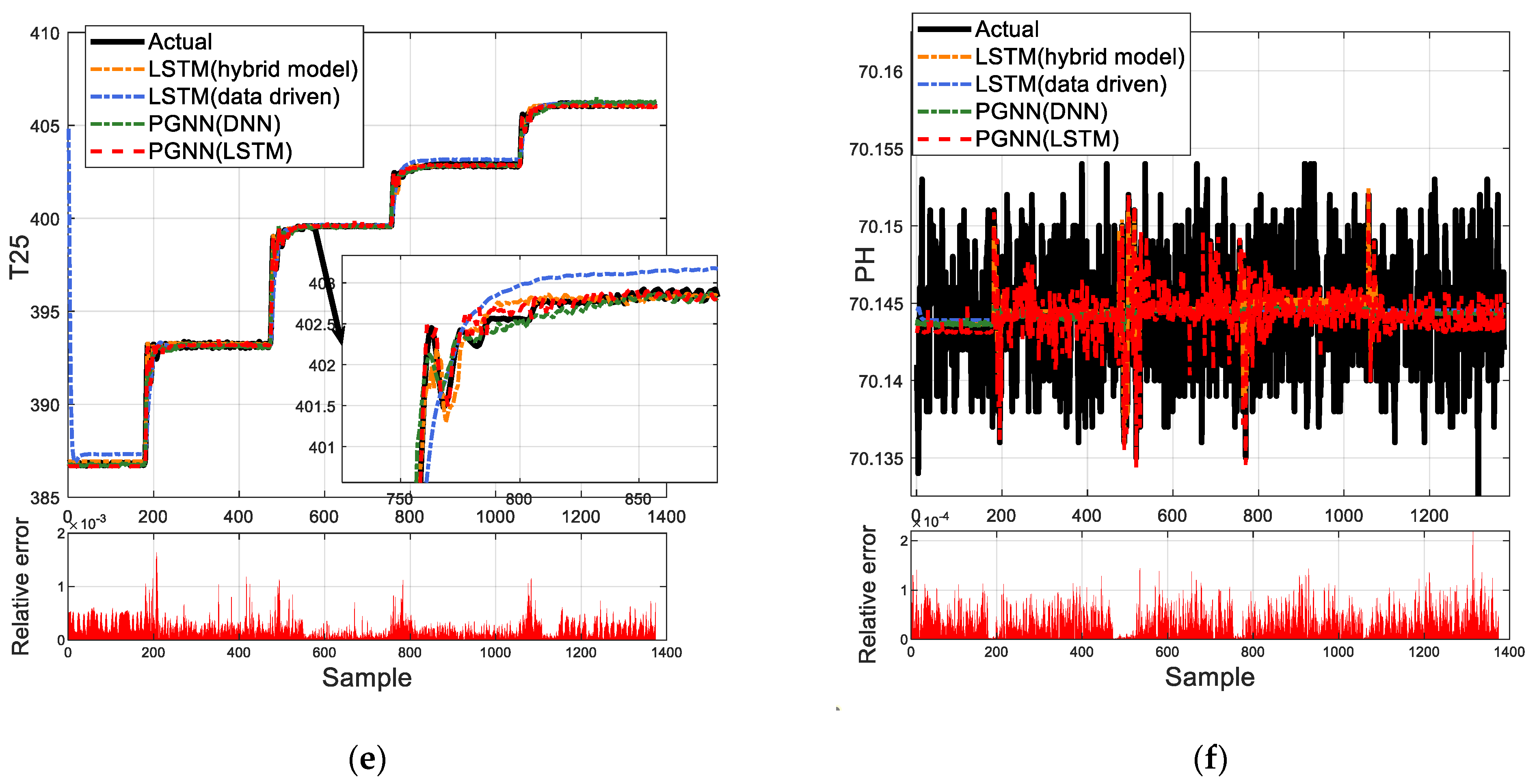
4.3.1. Prediction Results of the PGNN and Discussion

The data are normalized and preprocessed, and the PGNN network is trained on the basis of the Adam algorithm. After 400 iterations, the network’s loss function and root mean square error achieve a more desirable performance, with a training RMSE of 0.3061.
The prediction results of the PGNN model are shown in Figure 10a–f. A comparison of the predicted and actual values from the six sensors reveals that the overall prediction accuracy is high. For example, in the case of the N 1 sensor, the noise measurement standard deviation is 0.25% [7]. As can also be seen in Figure 10a, the relative error between the PGNN prediction and the actual value is basically below 0.25%, which does not exceed the measurement standard deviation of the N 1 sensor. Therefore, its prediction accuracy is within the permissible range, and the same is true for each sensor. In addition, the prediction error will significantly fluctuate when the throttle lever is being pushed, but will recover quickly.
A comparison of five classical approaches involving the LSTM (hybrid model), the LSTM (data-driven) model, and the PGNN (DNN) model is conducted to demonstrate the performance of the proposed model. To ensure fair quantitative comparisons, the three methods are tested using the same datasets and data partitioning methods as those used in Section 3.1.
A detailed description of these methods is necessary. The LSTM (hybrid model) and the LSTM (data-driven) model are both black-box models, but these two models have differences. The LSTM (hybrid model) is a model–data hybrid that uses the predicted output information of the model. It has 10 inputs, including 4 measured engine inputs and 6 predicted model outputs. The LSTM (data-driven) model is purely data driven, i.e., it only uses 4 measured inputs of the engines as inputs to the LSTM. It is to be noted that both methods use a purely data-driven learning objective.
The proposed method, called the PGNN(LSTM), refers to the fact that the LSTM is used as the basic neural network model in the PGNN. The PGNN (DNN) means that a deep neural network (DNN), instead of LSTM, is used as the basic network model in the PGNN. DNNs are the basic models of deep learning; they are neural networks with many hidden layers [22]. In particular, it is vital to illustrate that both the PGNN(LSTM) and PGNN (DNN) use a learning objective based on a physical loss function and model–data hybrid modeling.
The prediction results for each method are shown in Figure 10. The solid black lines are the actual engine measurements. The orange dashed lines are the predicted engine outputs from the LSTM (hybrid model). The blue dashed lines are the predicted engine outputs from the LSTM (data-driven) model. The green dashed lines are the predicted PGNN (DNN) engine outputs. The red dashed lines are the predicted PGNN(LSTM) engine outputs.
Using the N1 sensor as an example, the results in Figure 10a illustrate that all the methods can track the predicted output of the engine, but there are differences in their performances. What stands out in Figure 11 is that the LSTM (hybrid model) and the PGNN(LSTM) have a better tracking performance. The deviation between the predicted and observed values of these two models is small, which is reflected in the RMSE values. Near the 470th sample, the throttle lever was pushed and the engine output fluctuated. At this point, both the PGNN(LSTM) and the LSTM (hybrid model) tracked the fluctuations better. Looking at Figure 10, it is apparent that the predicted output of the PGNN (DNN) model differed significantly from the true value. This also reflects the superiority of the LSTM in handling data with a time dependence. Furthermore, Figure 10 shows that the prediction curves of the LSTM (data-driven) model converge far more poorly in the initial stage than the other methods, which is an interesting observation. More importantly, the LSTM (data-driven) model does not track the measured output of the engine well in either a steady state or under dynamic conditions. This reflects the importance of using physical information.
Figure 11 compares the quantitative values of the performances of the different models. A smaller RMSE value means that the training has a better prediction performance for the aeroengine parameters. An inspection of the data in Figure 11 reveals that the PGNN(LSTM) has the best performance in terms of the training and validation RMSEs, with a training RMSE of 0.3061 and a test RMSE of 0.9897. Another prediction method, the LSTM (hybrid model), has a training RMSE of 0.3255 and a test RMSE of 1.0596, which are at about the same level of performance as that of the method proposed in this paper. The physical bootstrap loss function in the PGNN(LSTM) provides a new way of training the proposed model. This is important for black-box models, because physical inconsistencies can lead to severe economic losses and safety accidents. The new loss function, which takes into account the laws of physics, is able to evaluate physical inconsistencies quantitatively, and physical inconsistencies hidden in the model parameters and target results are eliminated by prior physical knowledge, without affecting their bias.
The performance of the PGNN (DNN) model is inferior to that of the proposed method, with a training RMSE of 0.3482 and a test RMSE of 1.1271. This is because the PGNN model uses a DNN as the baseline model, which cannot model changes in time–series and is not well suited to processing time–series data. Instead, the PGNN model used in this paper uses an LSTM as the baseline model, which preserves the time–series nature of the data and therefore improves the prediction accuracy. Finally, the prediction model with the worst performance was analyzed. The LSTM (data-driven) model has a training RMSE of 1.0300 and a test RMSE of 1.6731. Only limited input information is provided to the LSTM (data-driven) model, meaning that the model uses the input as the engine input and does not use any physical knowledge (either the predicted output of the physical model or in the form of a physics-based loss function), leading to difficulties in ensuring the prediction accuracy. In the remaining three models, all of which use a mixed physical data modeling setup, the prediction accuracy is within acceptable limits and converges to the desired value quickly.
In summary, for the informants in this study, the PGNN(LSTM) model has a better prediction accuracy. This demonstrates the value of combining physical knowledge with data science models. The method proposed in this paper explores the hidden information of the physics and data, improving the prediction performance. The improved prediction accuracy facilitates subsequent fault identification, but the predicted value can be used as a virtual sensor and applied to fault tolerance strategies for control systems.
The computational times of the above four methods are summarized in Table 5. It can be observed that the PGNN(LSTM) model takes more training time than the other prediction models, because the PGNN(LSTM) model has more calculation steps. All three prediction models with an LSTM as the baseline model, namely the LSTM (hybrid model), the LSTM (data-driven) model, and the PGNN(LSTM) model, took longer to train than the PGNN (DNN) model. This is because the LSTM takes into account time–series relationships and has a more complex structure than the DNN. The test time of the PGNN(LSTM) model is within the acceptable limits. In the future, the architectures of the PGNN(LSTM) model should be optimized to reduce their computational time.

4.3.2. CNN Classification Results and Discussion

In order to evaluate the separability of the residual dataset more intuitively, the obtained fault feature dataset was processed using T-distributed Stochastic Neighbor Embedding (T-SNE) [58] and a principal component analysis (PCA) [59]. The distribution characteristics corresponding to the residual fault dataset are shown in Figure 12a,b, respectively, from which it can be seen that the coupling between each set of fault data is strong. As a deep learning method, CNNs have excellent advantages in dealing with such non-linear and highly correlated classification problems. Therefore, a CNN will be introduced to classify the residual dataset in the following section.
The engine control system has six measurement outputs: the low-pressure rotor speed N1, high-pressure rotor speed N2, high-pressure compressor outlet total pressure P31, low-pressure turbine outlet total pressure P6, high-pressure compressor inlet total temperature T25, and internal pressure P H . A fault classification CNN needs to be designed for the engine sensors. After continuous iterations, a CNN model with an acceptable performance is obtained.
The test data were used to validate the trained CNN, and Table 6 summarizes the classification performance of the proposed method, including its testing precision, recall, specificity, F1 score, accuracy, and total accuracy. It can be seen from the data in Table 6 that the total accuracy of the fault diagnosis is 95.9048%, which indicates the high diagnostic accuracy of the CNN. For the different fault types, the recall of short-circuit faults is 100%; open-circuit faults, 89.9%; bias faults, 87.4%; drift faults, 95.9%; pulse faults, 89.59%; periodic disturbance faults, 98.7%; and the normal state (i.e., no fault), 100%. Of these, the normal state and short-circuit faults perform well in all indicators, since both have more obvious characteristics and are better identified. The periodic disturbance faults are also easier to identify due to their more obvious frequency characteristics. The high levels of specificity and accuracy precision for each type of fault indicate a relatively low error rate in the classification. Overall, the obtained CNN achieves satisfactory results in terms of detecting and classifying sensor faults.
The confusion matrix is plotted in Figure 13 to more clearly describe the diagnostic capability of the fault diagnosis method proposed in this paper. The confusion matrix is a visual sketch of the classification effect. It describes the relationship between the true class properties of the sample data and the recognition results and is often used to evaluate the performance of classifiers. For example, there are 159 samples with a fault type labeled 1 in Figure 13 and 143 samples are correctly classified. The confusion matrix illustrates the significant advantages of the method proposed in this paper for aeroengine sensor fault diagnosis.

4.3.3. Comparison with Other Methods

To verify the superiority of the proposed PGNN(LSTM)–CNN model, it is compared with the LSTM (data-driven)–CNN and PGNN(LSTM)–SVM models. PGNN(LSTM)–SVM refers to a combination of a PGNN(LSTM) and a support vector machine (SVM). The comparison results of three methods are presented in Table 7. It can be seen that the proposed PGNN(LSTM)–CNN has better prediction and diagnosis results than the other methods. Taking the PGNN(LSTM)–CNN as an example, its test RMSE is 0.9897, test total accuracy is 95.90%, test total precision is 96.03%, test total recall is 95.99%, test F1 score is 96.00%, train time is 787 s, and test time is 1.84 s.
As shown in Table 7, the test RMSE of the PGNN(LSTM)–CNN and PGNN(LSTM)–SVM is 0.9897, which is higher than the 1.6731 of the LSTM (data-driven)–CNN. The results prove that the proposed PGNN(LSTM) is more reliable in reconfiguring the value of the engine’s sensors. The reason for this is that the PGNN(LSTM) takes into account both the physical model and the data drive, introducing a hybrid input strategy and a loss function based on physical information, compared to the data-driven LSTM.
A higher prediction accuracy means that the less information about changes in the dynamic operating conditions contained in the residuals, the less interference there is with the fault classification. Therefore, the proposed PGNN(LSTM), with a good prediction capability, can improve the fault diagnosis performance. The diagnosis result of the LSTM (data-driven)–CNN is found to be below 80%, which is almost 20% lower than that of the PGNN(LSTM)–CNN. As shown in Figure 10, the predicted and actual values of the LSTM (data-driven) model differed significantly in the initial stage of the prediction. This causes the residuals not to fluctuate around 0 and therefore adversely affects the diagnostic performance of the CNN. This suggests that prediction effects have an impact on the classification performance and that improving the prediction accuracy is necessary.
In addition, the proposed PGNN(LSTM)–CNN has a superior diagnosis performance to that of the other classification methods. The PGNN(LSTM)–CNN improved the classification performance by 10% over that of the PGNN(LSTM)–SVM in terms of the test total accuracy, the test total precision, the test total recall, and the test F1 score. In the PGNN(LSTM)–SVM, the residuals generated from the sensor readings and PGNN(LSTM)’s prediction are classified with the SVM. As a typical kernel-based learning algorithm, SVMs have gained a wide range of applications since they were proposed [17]. The diagnosis results of the SVM are below 90%, which illustrates that the CNN outperforms the SVM because of the strong fitting power that comes from the deep structure of the CNN.
Furthermore, although the PGNN(LSTM)–CNN approach achieves a higher prediction and classification performance than the other two methods, its model is also more complex. In the future, models with a more optimized internal structure but maintained performance should be developed to reduce the hardware resource consumption side.
It can be seen from the above discussion that the PGNN(LSTM)–CNN combines the advantages of hybrid inputs and a novel physical-based loss function and effectively uses the predictive time–series capability of an LSTM and the excellent classification capability of CNNs. This method has a superior diagnosis performance for engine sensors under dynamic conditions.

5. Conclusions

This paper proposed that a PGNN addresses the insufficiency of physics-based and data-driven models for the fault diagnosis of aeroengine control system sensors under dynamic conditions. The method innovatively solved the difficulties in the fault diagnosis due to the complexity of the engine operating conditions and the dynamic changes in the physical parameters. In summary:
(1)
A hybrid physics-data-based input strategy was proposed. After establishing a linear model of the engine based on physical principles, a hybrid information source, consisting of data and a priori knowledge, was formed by combining the physics-based model with historical engine data to fully exploit the implicit relationship between the input and output, improving the accuracy of the prediction.
(2)
The customized loss function included not only supervised losses, but also loss functions based on physical information. The physical-information-based loss function took into account known forms of physical relationships between the input and output of the engine. This loss function incorporated the physical knowledge into the PGNN model’s training process to eliminate physical inconsistencies in the parameters and prediction results, thus improving the performance of the PGNN.
(3)
An intelligent diagnosis method based on the PGNN–CNN was provided to solve the fault diagnosis problem of engine control systems under dynamic conditions. With a prediction–residual–fault classification structure, the effect of changing the engine flight conditions on the measured engine output was attenuated through residual generation. The proposed PGNN–CNN model was successful in diagnosing engine sensor faults.
It would be beneficial to provide deeper physical knowledge insights into neural network models. In future work, the integration of multi-physical field knowledge and data-mining techniques will be further investigated to enable the fault diagnosis and prediction of digital twin-based engines. Multiple-fault diagnoses and real-time diagnoses are also research directions to be considered in the future.

Author Contributions

Conceptualization, H.L. (Huihui Li), L.G. and H.L. (Huacong Li); methodology, H.L. (Huihui Li) and L.G.; software, H.L. (Huihui Li) and Z.L.; validation, H.L. (Huihui Li); formal analysis, H.L. (Huihui Li) and L.G.; investigation, H.L. (Huihui Li); resources, L.G. and Z.L.; data curation, L.G. and Z.L.; writing—original draft preparation, H.L. (Huihui Li) and Z.L.; writing—review and editing, L.G. and H.L. (Huacong Li); visualization, H.L. (Huihui Li); supervision, L.G.; project administration, L.G. All authors have read and agreed to the published version of the manuscript.

Funding

This research received no external funding.

Data Availability Statement

Public data have not been used and the self-acquired data set cannot been shared.

Conflicts of Interest

The authors declare no conflict of interest.

References

  1. Yao, H. Aero-Engine Full Authority Digital Electronic Control System; Aviation Industry Press: Beijing, China, 2014. [Google Scholar]
  2. Liu, Z.; Huang, Y.; Gou, L.; Fan, D. A robust adaptive linear parameter-varying gain-scheduling controller for aeroengines. Aerosp. Sci. Technol. 2023, 138, 108319. [Google Scholar] [CrossRef]
  3. Lv, C.; Chang, J.; Bao, W.; Yu, D. Recent research progress on airbreathing aero-engine control algorithm. Propuls. Power Res. 2022, 11, 1–57. [Google Scholar] [CrossRef]
  4. Cao, M.; Huang, J.Q.; Zhou, J.; Chen, X.; Lu, F.; Wei, F. Current status, challenges and opportunities of fault diagnosis and health management for civil aviation engines: Fault diagnosis and prediction of gas path, machinery and FADEC systems. Acta Aeronaut. 2022, 43, 9–41. [Google Scholar]
  5. Yu, H.; Zhu, J.T.; Sun, Z.S.; Gao, L.J. Sensor fault diagnosis of gas turbine engines using an integrated scheme based on improved least squares support vector regression. Proc. Inst. Mech. Eng. Part G J. Aerosp. Eng. 2019, 234, 607–623. [Google Scholar]
  6. Pourbabaee, B.; Meskin, N.; Khorasani, K. Sensor Fault Detection, Isolation, and Identification Using Multiple-Model-Based Hybrid Kalman Filter for Gas Turbine Engines. IEEE Trans. Control Syst. Technol. 2016, 24, 1184–1200. [Google Scholar] [CrossRef] [Green Version]
  7. Zhang, M. Data-Driven Aero-Engine Control System Sensor Fault Diagnosis Based on Data; Northwestern Polytechnic University: Fremont, CA, USA, 2023. [Google Scholar]
  8. Kobayashi, T.; Simon, D.L. Evaluation of an enhanced bank of Kalman filters for in-flight aircraft engine sensor fault diagnostics. J. Eng. Gas Turbines Power-Trans. ASME 2005, 127, 497–504. [Google Scholar] [CrossRef] [Green Version]
  9. Sun, R.Q.; Han, X.B.; Chen, Y.X.; Gou, L.F. Hyperelliptic Kalman filter-based aeroengine sensor fault FDIA system under multi-source uncertainty. Aerosp. Sci. Technol. 2023, 132, 08058. [Google Scholar] [CrossRef]
  10. Chen, J.; Patton, R.J.; Zhang, H.Y. Design of unknown input observers and robust fault detection filters. Int. J. Control 1996, 63, 85–105. [Google Scholar] [CrossRef]
  11. Gou, L.; Shen, Y.W.; Zheng, H.; Zeng, X.Y. Multi-Fault Diagnosis of an Aero-Engine Control System Using Joint Sliding Mode Observers. IEEE Access 2020, 8, 10186–10197. [Google Scholar] [CrossRef]
  12. Frank, P.M. Fault Diagnosis in Dynamic Systems using Analytical and Knowledge-Based Redundancy—A Survey and Some New Results. Automatica 1990, 26, 459–474. [Google Scholar] [CrossRef]
  13. Fu, W.J.; Sha, Y.D.; Yao, A.F. Research on aero-engine vibration fault diagnosis using wavelet analysis. J. Shenyang Inst. Aeronautcal Eng. 2008, 91, 11–14. [Google Scholar]
  14. Lei, Y.; Lin, J.; He, Z.; Zuo, M.J. A review on empirical mode decomposition in fault diagnosis of rotating machinery. Mech. Syst. Signal Process. 2013, 35, 108–126. [Google Scholar] [CrossRef]
  15. Shen, Y.; Li, L.L.; Wang, Z.H. A Review of Fault Diagnosis and Fault—Tolerant Control Techniques for Spacecraft. J. Astronaut. 2022, 41, 647–656. [Google Scholar]
  16. Huang, Y.; Tao, J.; Sun, G.; Wu, T.Y.; Yu, L.L.; Zhao, X.B. A novel digital twin approach based on deep multimodal information fusion for aero-engine fault diagnosis. Energy 2023, 270, 126894. [Google Scholar] [CrossRef]
  17. Zhao, Y.P.; Wang, J.J.; Li, X.Y.; Peng, G.J.; Yang, Z. Extended least squares support vector machine with applications to fault diagnosis of aircraft engine. ISA Trans. 2020, 97, 189–201. [Google Scholar] [CrossRef]
  18. Liu, R.; Yang, B.; Zio, E.; Chen, X. Artificial intelligence for fault diagnosis of rotating machinery: A review. Mech. Syst. Signal Process. 2018, 108, 33–47. [Google Scholar] [CrossRef]
  19. Baptista, M.L.; Prendinger, H. Aircraft Engine Bleed Valve Prognostics Using Multiclass Gated Recurrent Unit. Aerospace 2023, 10, 354. [Google Scholar] [CrossRef]
  20. Fink, O.; Wang, Q.; Svensén, M.; Dersin, P.; Lee, W.J.; Ducoffe, M. Potential, challenges and future directions for deep learning in prognostics and health management applications. Eng. Appl. Artif. Intell. 2020, 2020, 103678. [Google Scholar] [CrossRef]
  21. Zhang, Y.; Xin, Y.; Liu, Z.; Ma, G. Health status assessment and remaining useful life prediction of aero-engine based on BiGRU and MMoE. Reliab. Eng. Syst. Saf. 2022, 220, 108263. [Google Scholar] [CrossRef]
  22. Wen, X.; Xu, Z. Wind turbine fault diagnosis based on ReliefF-PCA and DNN. Expert Syst. Appl. 2021, 178, 115016. [Google Scholar] [CrossRef]
  23. Yan, B.; Qu, W. Aero-engine sensor fault diagnosis based on stacked denoising autoencoders. In Proceedings of the 2016 35th Chinese Control Conference (CCC), Chengdu, China, 27–29 July 2016. [Google Scholar]
  24. Gou, L.F.; Li, H.H.; Li, H.C.; Pei, X.N. Aeroengine control system sensor fault diagnosis based on CWT and CNN. Math. Probl. Eng. 2020, 2020, 5357146. [Google Scholar] [CrossRef] [Green Version]
  25. Tamilselvan, P.; Wang, P.F. Failure diagnosis using deep belief learning based health state classification. Reliab. Eng. Syst. Saf. 2016, 17, 1287–1304. [Google Scholar] [CrossRef]
  26. Willard, J.; Jia, X.; Xu, S.; Steinbach, M.; Kumar, V. Integrating scientific knowledge with machine learning for engineering and environmental systems. arXiv 2022, arXiv:2003.04919. [Google Scholar] [CrossRef]
  27. Arrieta, A.B.; Díaz-Rodríguez, N.; Del Ser, J.; Bennetot, A.; Tabik, S.; Barbado, A.; Garcia, S.; GilLopez, S.; Molina, D.; Benjamins, R.; et al. Explainable Artificial Intelligence (XAI): Concepts, taxonomies, opportunities and challenges toward responsible AI. Inf. Fusion 2020, 58, 82–115. [Google Scholar] [CrossRef] [Green Version]
  28. Karniadakis, G.E.; Kevrekidis, I.G.; Lu, L.; Perdikaris, P.; Wang, S.; Yang, L. Physics-informed machine learning. Nat. Rev. Phys. 2021, 3, 422–440. [Google Scholar] [CrossRef]
  29. Von Rueden, L.; Mayer, S.; Beckh, K.; Georgiev, B.; Giesselbach, S.; Heese, R.; Kirsch, B.; Pfrommer, J.; Pick, A.; Ramamurthy, r.; et al. Informed Machine Learning–A taxonomy and survey of integrating prior knowledge into learning systems. IEEE Trans. Knowl. Data Eng. 2021, 35, 614–633. [Google Scholar] [CrossRef]
  30. Minh, D.; Wang, H.X.; Li, Y.F.; Nguyen, T.N. Explainable artificial intelligence: A comprehensive review. Artif. Intell. Rev. 2022, 55, 3503–3568. [Google Scholar] [CrossRef]
  31. Diligenti, M.; Roychowdhury, S.; Gori, M. Integrating prior knowledge into deep learning. In Proceedings of the 2017 16th IEEE International Conference on Machine Learning and Applications (ICMLA), Cancun, Mexico, 18–21 December 2017; pp. 920–923. [Google Scholar]
  32. Xu, J.; Zhang, Z.; Friedman, T.; Liang, Y.; Van den Broeck, G. A semantic loss function for deep learning with symbolic knowledge. arXiv 2018, arXiv:1711.11157. [Google Scholar]
  33. Karpatne, A.; Watkins, W.; Read, J.; Kumar, V. Physics-guided neural networks (PGNN): An application in lake temperature modeling. arXiv 2017, arXiv:1710.11431. [Google Scholar]
  34. Stewart, R.; Ermon, S. Label-free supervision of neural networks with physics and domain knowledge. In Proceedings of the Thirty-First AAAI Conference on Artificial Intelligence, San Francisco, CA, USA, 4–9 February 2017; pp. 2576–2582. [Google Scholar]
  35. Wang, J.; Li, Y.; Zhao, R.; Gao, R.X. Physics guided neural network for machining tool wear prediction. J. Manuf. Syst. 2020, 57, 298–310. [Google Scholar] [CrossRef]
  36. Zamzam, A.S.; Sidiropoulos, N.D. Physics-aware neural networks for distribution system state estimation. IEEE Trans. Power Syst. 2020, 35, 4347–4356. [Google Scholar] [CrossRef] [Green Version]
  37. Chao, M.A.; Kulkarni, C.; Goebel, K.; Fink, O. Fusing physics-based and deep learning models for prognostics. Reliab. Eng. Syst. Saf. 2022, 217, 107961. [Google Scholar] [CrossRef]
  38. Shen, S.; Lu, H.; Sadoughi, M.; Hu, C.; Nemani, V.; Thelen, A.; Webster, K.; Darr, M.; Sidon, J.; Kenny, S. A physics-informed deep learning approach for bearing fault detection. Eng. Appl. Artif. Intell. 2021, 103, 104295. [Google Scholar] [CrossRef]
  39. Tidriri, K.; Chatti, N.; Verron, S.; Tiplica, T. Bridging data-driven and model-based approaches for process fault diagnosis and health monitoring: A review of researches and future challenges. Annu. Rev. Control 2016, 42, 63–81. [Google Scholar] [CrossRef]
  40. Du, X.; Chen, J.; Zhang, H.; Wang, J. Fault detection of aero-engine sensor based on inception-CNN. Aerospace 2022, 9, 236. [Google Scholar] [CrossRef]
  41. Lin, J.; Zhang, B.Y.; Zhang, D.Y. Research status and prospect of fault diagnosis for gas turbine aeroengine. Acta Aeronaut. Astronaut. Sin. 2022, 43, 626565. [Google Scholar]
  42. Huang, Y.; Sun, G.; Tao, J.; Hu, Y.; Yuan, L. A modified fusion model-based/data-driven model for sensor fault diagnosis and performance degradation estimation of aeroengine. Meas. Sci. Technol. 2022, 33, 085105. [Google Scholar] [CrossRef]
  43. Li, H.H.; Gou, L.F.; Chen, Y.X.; Li, H.C. Fault Diagnosis of Aeroengine Control System Sensor Based on Optimized and Fused Multidomain Feature. IEEE Access 2022, 10, 96967–96983. [Google Scholar] [CrossRef]
  44. Ding, S.; Yuan, Y.; Xue, N.; Liu, X. An onboard aeroengine model-tuning system. J. Aerosp. Eng. 2017, 34, 04017018. [Google Scholar] [CrossRef]
  45. Gao, W.; Pan, M.; Zhou, W.; Lu, F.; Huang, J.Q. Aero-Engine Modeling and Control Method with Model-Based Deep Reinforcement Learning. Aerospace 2023, 13, 209. [Google Scholar] [CrossRef]
  46. Jiang, Z.; Yang, S.; Wang, X.; Long, Y. An Onboard Adaptive Model for Aero-Engine Performance Fast Estimation. Aerospace 2022, 9, 845. [Google Scholar] [CrossRef]
  47. Gou, L.F.; Zeng, X.Y.; Wang, Z.; Han, G.; Lin, C.; Cheng, X. A linearization model of turbofan engine for intelligent analysis towards industrial internet of things. IEEE Access 2019, 7, 145313–145323. [Google Scholar] [CrossRef]
  48. Tan, M.; Yuan, S.; Li, S.; Su, Y.; Li, H.; He, F. Ultra-short-term industrial power demand forecasting using LSTM based hybrid ensemble learning. IEEE Trans. Power Syst. 2019, 35, 2937–2948. [Google Scholar] [CrossRef]
  49. Shen, K.; Zhao, D. An EMD-LSTM Deep Learning Method for Aircraft Hydraulic System Fault Diagnosis under Different Environmental Noises. Aerospace 2023, 11, 55. [Google Scholar] [CrossRef]
  50. Agarap, A.F. Deep learning using rectified linear units (relu). arXiv 2018, arXiv:1803.08375. [Google Scholar]
  51. Sutskever, I. Training Recurrent Neural Networks; University of Toronto: Toronto, ON, Canada, 2013. [Google Scholar]
  52. Li, D.; Wang, Y.; Wang, J.X.; Wang, C.; Duan, Y. Recent advances in sensor fault diagnosis: A review. Sens. Actuators A Phys. 2020, 309, 11199. [Google Scholar] [CrossRef]
  53. Jiao, J.; Zhao, M.; Lin, J.; Liang, K. A comprehensive review on convolutional neural network in machine fault diagnosis. Neurocomputing 2020, 417, 36–63. [Google Scholar] [CrossRef]
  54. Zhao, B.; Zhang, X.; Li, H.; Yang, Z. Intelligent fault diagnosis of rolling bearings based on normalized CNN considering data imbalance and variable working conditions. Knowl. Based Syst. 2020, 199, 105971. [Google Scholar] [CrossRef]
  55. Li, H.; Gou, L.; Zheng, H.; Li, H.C. Intelligent Fault Diagnosis of Aeroengine Sensors Using Improved Pattern Gradient Spectrum Entropy. Int. J. Aerosp. Eng. 2021, 2021, 1–20. [Google Scholar] [CrossRef]
  56. Yang, T.L.; Chen, J.J.; Zheng, Q.G. Real Time Verification of Hardware-in-the-Loop for Aeroengine Component Level Model. Aeroengine 2021, 47 (Suppl. 1), 76–84. [Google Scholar]
  57. Alpaydin, E. Neural Networks and Deep Learning. In Machine Learning: The New AI; MIT Press: Cambridge, MA, USA, 2016. [Google Scholar]
  58. Van der Maaten, L.; Hinton, G. Visualizing data using t-SNE. J. Mach. Learn. Res. 2008, 9, 2579–2605. [Google Scholar]
  59. Verbanck, M.; Josse, J.; Husson, F. Regularised PCA to denoise and visualise data. Stat. Comput. 2015, 25, 471–486. [Google Scholar] [CrossRef] [Green Version]
Figure 1. The framework of a PGNN.
Aerospace 10 00644 g001
Figure 3. Structural sketch of the aeroengine model.
Aerospace 10 00644 g003
Figure 4. The schematic diagram of a PGNN.
Aerospace 10 00644 g004
Figure 5. The architecture of the basic LSTM.
Aerospace 10 00644 g005
Figure 6. Typical CNN structure.
Aerospace 10 00644 g006
Figure 7. The scheme for the PGNN and CNN structure.
Aerospace 10 00644 g007
Figure 8. Time domain signal of the sensor. (a) Fault-free sensor signals; and (b) Faulty sensor signals.
Aerospace 10 00644 g008
Figure 9. The sensor signals for seven health conditions.
Aerospace 10 00644 g009
Figure 10. Prediction results. (a) N 1 Sensor; (b) N 2 Sensor; (c) P 31 Sensor; (d) P 6 Sensor; (e) T 25 Sensor; and (f) P H Sensor.
Aerospace 10 00644 g010aAerospace 10 00644 g010b
Figure 11. PGNN prediction results.
Aerospace 10 00644 g011
Figure 12. Data visualization results. (a) PCA; and (b) T-SNE.
Aerospace 10 00644 g012
Figure 13. The confusion matrix.
Aerospace 10 00644 g013
Table 1. Input and output parameters.
The Input of the PGNN
NumberName
1LM
2D8
3A1
4A2
5 N ^ 1 , m
6 N ^ 2 , m
7 P ^ 31 , m
8 P ^ 6 , m
9 T ^ 25 , m
10 P ^ H m
The output of the PGNN
NumberName
1 N ^ 1
2 N ^ 2
3 P ^ 31
4 P ^ 6
5 T ^ 25
6 P ^ H
The output of the CNN
NumberName
1Residual
The output of the CNN
NumberName
1Fault diagnosis results
Table 2. Types and labels of N1 sensor faults.
Fault TypeCause of FaultLabel
Short-circuit faultPollution caused by the bridge road corrosion line short connection1
Open-circuit faultBroken signal line or an unconnected chip pin 2
Bias faultBias current or bias voltage3
Spike fault Random interference, surge, spark discharge in power and ground, D/A converter
burr in the converter, etc.
4
Drift faultTemperature drift5
Periodic disturbance faultPower interference or voltage instability6
Normal----7
Table 3. PGNN network structure parameters.
Network Layer TypeParameter Value
Input layer10
LSTM1 hidden layer128
Dropout1 layer20%
LSTM2 hidden layer64
Dropout2 layer10%
Fully connected layer50
Output layer6
Maximum number of iterations400
Parameter update methodAdam
Learning rate0.005
Learning rate decline factor0.2
Learning rate decrease period125
Table 4. CNN structure parameters.
Network LayerOutput
Input layer1 × 500 × 1
Convolutional layer C16 filter (size = 5 × 5, slide = 1)
Pooling layer P116 filter (size = 2 × 2, slide = 1)
Convolutional layer C2 6 filter (size = 5 × 5, slide = 1)
Pooling layer P216 filter (size = 2 × 2, slide = 1)
Fully connected layer 120
Dropout0.5
Softmax layer1 × 7
Maximum number of iterations2000
Learning rate0.001
Table 5. Computational time of different methods.
MethodLSTM
(Hybrid Model)
LSTM
(Data-Driven)
PGNN (DNN)PGNN (LSTM)
Training time (s)38538128.15427
Test time (s)0.470.470.110.4926
Table 6. Test diagnostic results of the CNN.
Fault TypePrecisionRecallF1 ScoreAccuracy Specificity
1Short-circuit fault100%100%100%100%100%
2Open-circuit fault88.3%89.9%89.1%96.7%97.9%
3Bias fault88.0%87.4%87.7%96.5%98.0%
4Spike fault100%95.9%97.9%99.4%100%
5Drift fault100%100%100%100%100%
6Periodic disturbance fault98.0%98.7%98.4%99.5%99.7%
7Normal97.8%100%98.9%99.7%99.7%
Total accuracy95.9%
Table 7. Comparison between different methods.
Fault TypeLSTM (Data-Driven)–CNNPGNN (LSTM)–CNNPGNN (LSTM)–SVM
Test RMSE1.67310.98970.9897
Test total accuracy77.62%95.90%85.33%
Test total precision77.53%96.03%88.59%
Test total recall 77.40%95.99%85.44%
Test F1 score77.40%96.00%85.64%
Train time(s)741787431.5
Test time(s)1.331.843.85
Disclaimer/Publisher’s Note: The statements, opinions and data contained in all publications are solely those of the individual author(s) and contributor(s) and not of MDPI and/or the editor(s). MDPI and/or the editor(s) disclaim responsibility for any injury to people or property resulting from any ideas, methods, instructions or products referred to in the content.

