Abstract
To deal with the attitude tracking control problem of a struck or pierced geocentric polar displaced solar sail (GPDSS), an attitude adaptive control strategy is proposed in this paper under the complex conditions of unknown inertial parameters, external disturbance and input saturation. First, on the basis of a flexible solar sail spacecraft attitude dynamics model with damping terms and vibration initial values, an integrated disturbance term, including inertial parameter uncertainties and external disturbance, is constructed. Second, a radial basis function neural network is applied to design a disturbance estimator with an adaptive law to estimate the integrated disturbance in real time. Then, a sliding-mode controller with fixed-time convergence in the reach phase and finite-time stability in the sliding phase is designed, and stability analysis is conducted by using the Lyapunov theory. Finally, comparative simulations with a linear sliding-mode controller and numerical simulations under various workings are performed. The results show that the designed adaptive control strategy can effectively achieve the attitude tracking control of the GPDSS.
1. Introduction
Polar regions are newly being affected, resulting in the world’s sustainable development and human survival, which are both strategic commanding heights for future competition between interests and influence of major powers [1]. Due to their location, polar regions are the site of major scientific research in six dimensions. The need for communication, data relay, weather forecasting and other services in polar regions has become very urgent, so the task of designing polar displaced orbits has begun [2]. Driver [3] was the first to propose the concept of polar displaced orbit; he studied and analyzed relationships between the control forces of a polar displaced spacecraft in terms of its time and altitude.
Polar displaced solar sails are always controlled using three-axis stabilization, whereas a solar sail for triaxial stabilization is generally a square sail with booms [4]. So far, there are three main ways to obtain torque for attitude control studies of solar sails [5,6]: adjusting the center of mass (including sliding masses [7,8,9,10] and gimbaled masses [11,12,13,14]); adjusting the center of pressure (including sail panel translation/rotation [15,16,17,18,19,20,21,22], control vanes [23,24] and reflectivity modulation [25,26,27,28,29,30]); and passive stability design (seeking to stabilize solar sail geometry in the presence of SRP [31,32]).
The attitude control methods mentioned above have not been effectively verified except for reflectivity modulation. There are two directions of development of attitude control methods for solar sails: on the one hand, various existing attitude control methods can be combined to compensate for each other’s disadvantages; on the other hand, new attitude control systems can be developed by introducing smart materials or other latest technologies [4]. Since hybrid propulsion systems have the advantage of no propellant consumption and are able to overcome the disadvantages of solar sails, which cannot provide the propulsive component of the spacecraft pointing towards the Sun, complex attitude control missions can be performed using hybrid propulsion technology [33].
SpaceX’s latest launch of the Starlink satellite “V2 mini” featured an argon Hall thruster with a thrust of 170 mN and a mass of only 2.1 kg. This makes it possible to achieve hybrid attitude control without significantly increasing the mass of the solar sail spacecraft. Compared with the existing xenon or krypton thrusters, the biggest advantage of argon electric thrusters is their extremely low cost. High-purity xenon gas used in xenon electric propulsion costs tens of thousands of CNY for 1 kg, whereas 1 kg of high-purity argon gas costs only a few CNY [34]. However, to prevent the failure of propellant-free actuators and avoid adding too much mass to the solar sail spacecraft, we use propellant-free actuators as the primary means of attitude control, supplemented by argon Hall thrusters.
To study the attitude control system of the solar sail, the structure of the solar sail must be clearly understood. After all, the structure of the vehicle is the subject of the action of the control system. Therefore, it is necessary and meaningful work to investigate the design solutions for a solar sail spacecraft. A fully deployed and orbiting solar sail spacecraft has the following four characteristics [35,36]:
- Although the mass of a solar sail is not too large, its special type of structure makes the overall dimensions very large, resulting in a solar sail spacecraft with a large rotational inertia.
- The flight time of a solar sail in polar displaced orbit would be very long, typically at least 2 years.
- Solar sails have the characteristics of high flexibility and low frequency and are prone to system vibration due to slight disturbances in the space environment.
- During ultra-long flight periods, there will be a huge disturbance torque, which is mainly caused by installation errors during the final assembly process of a large-sized solar sail spacecraft, deformation of the sail surface after orbiting and unfolding, and so on [37,38,39].
In addition, the environment of a polar displaced orbit is relatively harsh; for example, a large sail surface can result in the possibility of the sail surface being struck or pierced by star dust. For a 100 m × 100 m solar sail spacecraft with an SRP of 0.09 N and a pressure center offset of ±0.1 m, the in-flight SRP disturbance moment is ±0.009 Nm. According to the experimental data, if a 10,000 m2 solar sail undergoes a 6-year interstellar voyage, the solar sail will be pierced by interstellar dust amounting to about 2 million small holes, the area of which is about 1.5% of the entire sail surface [40]. This has little impact on the flight of the solar sail, but for the geocentric polar displaced solar sail (GPDSS), the attitude control stability will be significantly reduced, which in turn will affect the orbit. Therefore, it is not suitable for simulation analysis with the perturbation values used in the literature such as in [41,42].
Zhang et al. discovered a new type of graphene material in 2015 [43], which has the potential to increase the thrust of solar sails.
At present, the attitude control methods for polar displaced solar sails mainly include feedback control [44], PID control, adaptive control, sliding mode control [30], fuzzy control [45] and linear quadratic regulator control [19]. Bassetto et al. proposed a variable structure state feedback sliding mode control [30]. Chen et al. introduced neural network modeling and an automatic design method to solve the problems of lack of a priori knowledge and high manual workload in the design of fuzzy logical controller [45].
This article studies the attitude tracking control problem of a GPDSS after being struck or pierced under complex perturbations from multiple sources, such as unknown inertial parameters, external disturbances and input saturation. One nominal attitude of the polesitter satellite is applied to study the problem and nothing else is involved. The main contents include the following: the inertial uncertainty is separated from the nominal parameters as a disturbance term, and then its composition with external disturbance is used to construct the integrated disturbance term; a radial basis function (RBF) neural network is applied to design a disturbance estimator, which is used to estimate (based on an online adaptive law) and compensate for the constructed integrated disturbances in real time; a sliding-mode controller with fixed-time convergence and finite-time stability is designed; and the effectiveness of the proposed attitude control strategy is verified by a comparative simulation with a linear sliding-mode controller and simulations under different working conditions.
2. Attitude Dynamics Model of a GPDSS
The Earth’s orbit around the Sun is an ellipse with low eccentricity. When the displaced orbit deviates from the Sun–Earth line, as shown in Figure 1, the condition for generating the displaced orbit is that the normal direction of the solar sail must be consistent with the Z direction.
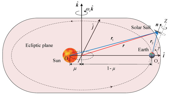
Figure 1.
Schematic diagram of Sun–Earth solar sail CR3BP.
A schematic diagram of the polar displaced orbit of a solar sail in the Earth coordinate system is shown in Figure 2. This is a non-Keplerian orbit in the form of a spiral.
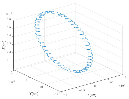
Figure 2.
Schematic diagram of the polar displaced orbit of a solar sail in the Earth coordinate system.
Figure 3 shows the ontological coordinate system of the solar sail. The origin is located at the center of mass of the solar sail spacecraft. The -axis is parallel to the normal direction of the sail surface and deviates from the direction of the Sun. The -axis points towards the direction of the boom connected to end point 1 on the sail surface. The -axis and the other two axes together form a right-handed right-angle coordinate system. The -axis is defined as the roll axis of the GPDSS, and the -axis and -axis are defined as the pitch and yaw axes, respectively.
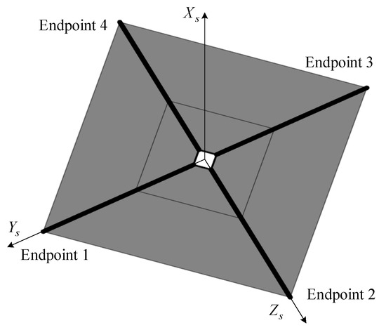
Figure 3.
The ontological coordinate system of the solar sail.
Attitude kinematics equation of the GPDSS:
where denotes the attitude angle of the solar sail obtained from the ontological coordinate system with respect to the inertial coordinate system. The rotational velocity of the attitude relative to the reference coordinate system can be expressed in the ontological coordinate system as: .
Decoupling the attitude orbit coupling dynamics equation, the attitude dynamics equation of the GPDSS is obtained as:
where ; is the rotational inertia when the solar sail is considered to be a rigid body; is the change in rotational inertia caused by the vibration of the sail surface; is the attitude stabilization control torque; is the external disturbance torque of the GPDSS; is the vibration mode of the sail surface ( is the order); is the parameter matrix related to ; and the stiffness matrix can be expressed as . The specific expressions and data of other related parameters are shown in Appendix A.
The components and assembly of the adopted propellant-free actuator are shown in Figure 4. When the propellant-free actuator is operating, the slider sliding on the support rod will change the center of mass of the spacecraft sail surface, and the pitch and yaw axis torques will be generated by adjusting the center of mass/pressure deviation. The rotation of the telescoping rod will rotate the spinnaker and thus change the center of pressure of the solar sail, and the rolling axis torque will be generated by adjusting the mass/pressure center deviation. The magnification of the rolling axis torque can be changed by adjusting the telescoping pole length. Due to the use of a propellant-free actuator, the control torque is quite limited. Moreover, in the current research on solar sails, the delay problem of the actuator is particularly prominent. For example, if the attitude is controlled by reflectivity modulation, the time delay can reach 20~30 s, whereas the time delay of chemical thrusters generally does not exceed 0.04 s. The sail surface of a GPDSS is a huge sail surface of tens of thousands of square meters. A small disturbance can bring about a chain of adverse reactions if it cannot be controlled in time.
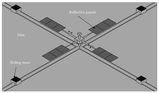
Figure 4.
Structural schematic diagram of the propellant-free actuators from.
Therefore, to ensure the rapid and stable attitude control of the GPDSS, a hybrid control strategy of propellant-free actuators and electric thrusters is suitable for engineering purposes. For example, fixing a thruster with a maximum thrust of 100 mN at the end point of the boom, which is 100 m long, can produce a maximum torque of . And according to Equation (32), it can be deduced that a 5 kg slider can only produce less than torque. Even so, the control torque available is still limited but more effective than a single propellant-free actuator. Here, assuming there is an upper limit for the control torque, its input saturation is:
Transforming Equation (2), we obtain:
When substituting into the above equation, the attitude kinematics and dynamics model are organized as follows:
where is the integrated disturbance term constructed from the external disturbance and the change in rotational inertia caused by the sail surface vibration.
3. Attitude Tracking Controller Design
If the desired angular velocity and attitude angle of the geocentric polar displaced solar sail are recorded as and , respectively, the attitude tracking error is:
By deriving the above equation and substituting it into the kinematic model (5), we obtain:
Similarly, the angular velocity error and its first-order derivative are:
Defining , Equation (5) can be rewritten as:
where is a nonlinear function; is a control input; and is the disturbance.
The designed sliding surface is [30]:
where ; , and denote adjustable slip surface coefficients, , ; and .
Deriving for , we have:
where .
Substituting Equations (5) and (8) into Equation (11), we obtain:
3.1. RBF Neural Network Disturbance Estimator Design
A disturbance estimator is designed by the RBF neural network to approximate . As shown in Figure 5, there are three layers of an RBF neural network. If the hidden layer includes enough neurons, the RBF can approximate any continuous function with an arbitrary accuracy and is a neural network with good local nonlinear approximation [46].
The activation function of neurons in the hidden layer consists of radial basis functions [47]. There is a central vector for each hidden layer node, whose dimension is equal to that of the input parameter vector . High-precision attitude angle and angular velocity information can be directly measured by measurement elements such as the star sensor and gyroscope, respectively, even if there are measurement errors., , is considered to be the Euclidean distance between them, and is the number of nodes in the hidden layer.

Figure 5.
Block diagram of the RBF network.
The hidden layer’s output consists of the nonlinear activation function :
where represents that the width of the Gaussian basis function, which is a positive scalar.
The integrated disturbance is approximated by the RBF neural network.
where represents the ideal RBF network weight and denotes the approximation error, which is a very small real vector satisfying . is the error upper bound.
The actual output of the disturbance estimator is:
Those marked with “^” indicate estimated values. To ensure the convergence of the errors and the real-time estimation, a reasonable adaptive law based on Lyapunov’s stability theory will be designed for in Section 3.3.
The disturbance estimation error is obtained from Equations (14) and (15):
where .
3.2. Control Law Design
The convergence law is chosen as follows:
where ; ; ; ; . , , and are the adjustable parameters.
From Equations (12) and (17), the control law is obtained as follows:
The closed-loop attitude tracking control system of GPDSS designed in this paper is shown in Figure 6.
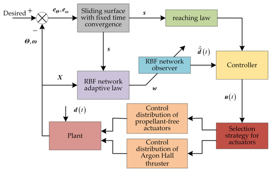
Figure 6.
Block diagram of the closed-loop attitude control for solar sails.
3.3. Stability Analysis
Assumption 1.
Assume that the rotational inertia of the solar sail is when it is considered as a rigid body, and the change in the rotational inertia of the solar sail due to the vibration of the sail surface is . is a small amount compared to .
Assumption 2.
The movement of the actuator does not have a direct effect on the vibration of the sail surface.
Assumption 3.
is an invertible matrix.
Assumption 4.
Assuming that under normal attitude control, the attitude angular velocity of the solar sail is a small amount.
Lemma 1 ([48]).
For any given real number () and constant , there is the following conclusion.
Lemma 2 ([49]).
For a nonlinear system , assuming the existence of a positive definite function , this satisfies:
where ; ; ; and is the normal number and the nonlinear system is fixed-time convergence. The state converges at a fixed time to the set of residuals.
The bound on the convergence time which is required to reach into is:
Lemma 3 ([50]).
For a nonlinear system , assuming the existence of a positive definite function , this satisfies:
where ; ; ; and and the nonlinear system is finite-time stable.
The settling time can be given by:
Theorem 1.
For the attitude dynamics system (5) of a GPDSS, if its control law is designed as Equation (18), and if the values of the parameters, such as , , , , , , and , are appropriate, the closed-loop system can converge to the sliding-mode surface in a fixed-time and stabilize to a small neighborhood near zero in finite-time, achieving the tracking of reference instructions.
Proof of Theorem 1.
The proof process will be divided into two steps. Step 1 proves that the system state converges to the sliding-mode surface at a fixed-time, and Step 2 proves that after reaching the sliding-mode surface, is stable in finite-time in a small neighborhood near zero.
- Step 1. The Lyapunov function is chosen as follows:
Deriving Equation (23) and substituting Equations (12) and (16) into it, we obtain:
The adaptive law can be designed as follows:
where represents the pseudo-converse operation.
From Equation (23), it follows that .
Substituting Equation (25) into Equation (24), and then from Lemma 1, we obtain:
where ; .
From Lemma 2, the closed-loop system converges to the sliding-mode surface at a fixed time. Additionally, the convergence time satisfies:
Step 2. The system reaches the sliding surface, .
The Lyapunov function is chosen as follows:
Deriving Equation (28) yields:
Since the attitude angle varies around and varies around , is a positive definite. Then, is also a positive definite and bounded.
From Lemma 3, is stabilized in a small neighborhood near zero in finite-time, and the stabilization time is:
where ; ; and .
This completes the Proof of Theorem 1. □
3.4. Control Variable Conversion
When the solar electric thruster is not operating, the actuator provides the required attitude control torque to the controller through slider motion and spinnaker rotation. The displacement of the slider and the angle of rotation of the spinnaker are the actuator variables. Record the attitude controller output as .
For the pitch and yaw axes, the structural design limits the range of motion of each slider due to the use of rigid light beam. The displacement of the slider can be obtained from the following equation [44]:
where is the pressure of sunlight; is the mass of each slider; is the total mass of the solar sail spacecraft; is the area of the solar sail surface; is the angle between the solar radiation pressure vector and the normal vector of the sail surface; is a small positive number.
Fixing the length of the telescopic boom, the turning angle of the spinnaker is:
where is the length of the telescopic boom; is the area of the spinnaker.
The basic thinking of controlling allocation: the maximum torque that can be generated by the propellant-free actuator is used as the threshold value. If the required control torque for solar sail spacecraft attitude control is less than the threshold, attitude control is performed by the propellant-free actuator. If it is greater than the threshold, attitude control is performed with thrusters only.
4. Simulation Results and Discussion
4.1. Simulation Conditions
In this section, numerical simulations are performed using the designed controller, based on the attitude dynamics of the GPDSS, to verify the effectiveness of the proposed method. The solar sail spacecraft is located in a levitating orbit 160,000 km from the geocentric with a large solar pressure acceleration of 15.8 mm/s2.
The number of vibration mode order is three.
Due to the large sail surface, the response time interval between the argon Hall thruster and propellant-free actuator is large, so the actuator is selected by setting a control threshold in each channel. The upper limit of the control torque (ULCT) of the argon Hall thruster is set to ; the ULCT of the slider is set to ; and the ULCT of the vanes is set to . The threshold value of the control torque of the rolling axis is set to , and the control torque threshold values of the pitch and yaw axes are set to . When the threshold value is exceeded, switch to an argon Hall thruster.
The relevant parameters of the sliding surface and controller are as follows:
The relevant characteristic parameters are outlined in Table 1.

Table 1.
Graphene-solar-sail-related characteristics parameters.
The parameters associated with the RBF neural network estimator are ,
We set the time-varying disturbance according to the disturbance magnitude as:
Vibration modes:
(1) Desired vibration modes: , ;
(2) Initial state: , . This corresponds to a lateral deformation of .
4.2. Simulation Results and Analysis
Since being pierced or struck happens in a very short space of time, its persistence is not considered here.
- Case 1: there are small initial state errors.
The initial angular velocity and attitude angle of the GPDSS are as follows:
The rotational inertia uncertainty due to sail surface vibration is set to:
The simulation results of Case 1 are shown in Figure 7, Figure 8, Figure 9, Figure 10, Figure 11, Figure 12 and Figure 13.
Figure 7 and Figure 8, respectively, describe the error tracking characteristics of the attitude angle and attitude angular velocity of a GPDSS for Case 1. The attitude angle error converges to a smaller range within 400 s, and the attitude angular velocity error converges to a small neighborhood near 0 within approximately 360 s. When the solar sail stabilizes, the tracking accuracy of the attitude angle is less than , and the tracking accuracy of attitude angular velocity is less than rad/s.

Figure 7.
Simulation results for the attitude errors (Case 1).

Figure 8.
Simulation results for the angular velocity error (Case 1).

Figure 9.
Simulation results for the sliding-mode surfaces (Case 1).

Figure 10.
Simulation results for the displacements of the slider and the angle of rotation of the spinnaker (Case 1).

Figure 11.
Simulation results for the disturbance estimation errors (Case 1).

Figure 12.
Simulation results for the vibration modes (Case 1).

Figure 13.
Simulation results for the modal velocities (Case 1).
Figure 9 describes the variation curve of the sliding surface. The sliding surface converges to a small neighborhood near 0 within about 300 s. Figure 10 describes the variation curve of the displacement of the slider and the angle of rotation of the spinnaker. During the convergence phase, the spinnaker angle oscillates between −0.75° and −0.65°, whereas the slider displacement oscillates between 5.3 m and 5.7 m. This is due to the presence of external disturbances.
Figure 11 describes the observation error curve of the disturbance estimator. The observation error gradually decreases until it converges to near zero, and the disturbance estimate approximates the true value, indicating the effect of the designed estimator with a sound perturbation estimation.
Figure 12 and Figure 13, respectively, describe the variation characteristics of the vibration mode and modal velocity of the GPDSS. When the initial value of the vibration is known, the vibration modes and modal velocities can converge to a smaller range within about 3 h and show fluctuations. The third-order vibration mode has a faster convergence speed, requiring about 0.12 h to converge, whereas the first- and second-order modes converge more slowly, and the convergence process undergoes large oscillation. In the stable state, the stabilization accuracy of the first- and second-order modes is less than , the stabilization accuracy of the third-order mode is less than and the modal velocity is less than .
- Case 2: there are large initial state errors.
The initial angular velocity and attitude angle of the GPDSS are as follows:
The rotational inertia uncertainty due to sail surface vibration is set to:
The simulation results of Case 2 are shown in Figure 14, Figure 15, Figure 16, Figure 17, Figure 18 and Figure 19.
Figure 14 and Figure 15, respectively, describe the error tracking characteristics of the attitude angle and attitude angular velocity for Case 2. The attitude angle error converges to a smaller range within 400 s, and the attitude angular velocity error converges to a small neighborhood near 0 within 400 s. This is different from the convergence time of the angular velocity error in Case 1 mainly because of the poor initial state of the angular velocity and attitude angle in Case 2. When the solar sail stabilizes, the tracking accuracy of the attitude angle is less than , and the tracking accuracy of the attitude angular velocity is less than rad/s, which is the same as the accuracy in Case 1.

Figure 14.
Simulation results for the attitude errors (Case 2).

Figure 15.
Simulation results for the angular velocity error (Case 2).

Figure 16.
Simulation results for the sliding-mode surfaces (Case 2).
Figure 16 describes the variation curve of the sliding surface. The sliding-mode surface converges to a small neighborhood near 0 within 300 s. Approximating the convergence time of the sliding surface in Case 1, it is indirectly verified that the controller is fixed-time convergent and finite-time stable.

Figure 17.
Simulation results for the control torques (Case 2).

Figure 18.
Simulation results for the disturbance estimation errors (Case 2).

Figure 19.
Simulation results for the lateral deformations at the endpoint 1 (Case 2).
Figure 17 describes the variation curve of the displacement of the slider and the angle of rotation of the spinnaker. After the control torque of the three axes exceeds the threshold of the propellant-free actuator, the argon Hall thruster is used.
Figure 18 describes the observation error curve of the disturbance estimator for Case 2. The observation error also decreases until it converges to a small range. However, it can be seen from the figure that there are obvious vibrations in the convergence section. This is due to the rapid change in the angular velocity of the solar sail, which results in the sustained high-frequency small-amplitude vibrations of the flexible structure.
Figure 19 describes the variation in the lateral deformation at endpoint 1 of the GPDSS for Case 2. With known initial lateral deformation, it can converge to a smaller range after about 4 h. The stability accuracy of the lateral deformation at endpoint 1 is less than m. The lateral deformation at endpoint 1 in Case 1 stabilizes significantly faster compared to Case 2 due to its smaller angular velocity because if the attitude adjustment process of the sail surface is gentle, it is relatively unlikely to excite the vibration of the flexible components.
- Case 3: Comparison simulation with a controller designed from a linear sliding surface.
Remark 1.
ASMC: adaptive sliding-mode controller (proposed in this paper). LSMC: linear sliding-mode controller (designed by the linear sliding-mode surface). NSMC: nonlinear sliding-mode controller (proposed in the literature [45]). IFLC: intelligent fuzzy logical controller (proposed in the literature [30]).
To further verify the performance of the ASMC, a comparison simulation was performed. The simulation results are shown in Figure 20, Figure 21 and Figure 22.
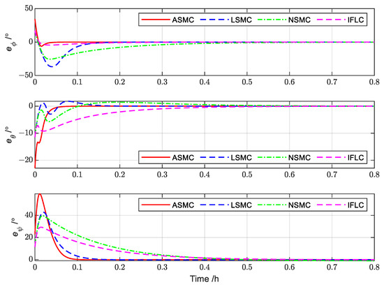
Figure 20.
Control attitude error comparison of different controllers.
Figure 20 describes the comparative simulation variation curve of the attitude angle error. From the simulation results, it can be found that the attitude angle error convergence variation curve of ASMC is smoother, with a faster convergence compared with other controllers. Figure 21 describes the comparative simulation variation curve of the attitude angular velocity error. As we found, the angular velocity errors of LSMC, NSMC and IFLC converge to a small value and then converge slowly, which is one of the main reasons for the slow convergence of the attitude angular error.

Figure 21.
Control angular velocity error comparison of different controllers.

Figure 22.
Comparison curves for the lateral deformations at the endpoint 1.
Figure 22 describes the comparative simulation variation curve for the lateral deformations at the endpoint 1. As we found, the convergence time of ASMC is basically the same as the convergence time of other controllers. During the convergence process, the vibration is more obvious under the action of LSMC, NSMC and IFLC, respectively. Compared with IFLC, NSMC and LSMC, which relies on its own robustness against disturbances, ASMC can use the designed disturbance estimator to achieve real-time control compensation, so the ASMC has higher stability accuracy.
5. Conclusions
In this paper, we studied the attitude tracking control problem of a struck GPDSS under multi-source complex perturbations such as unknown inertial parameters, external disturbance and input saturation. The simulation results verified the effectiveness of the designed sliding-mode controller. Additionally, compared with the linear controller, it broadened the application conditions, improved the control efficiency and met the attitude control task requirements of high stability, high precision and fast adjustment of the GPDSS. However, a situation where some information is unknown was not considered; therefore, an analysis of the time-varying effects of elastic modes on system parameters, the nonlinear effects on attitude dynamics and the study of intelligent materials to suppress vibrations will be subsequently carried out.
Author Contributions
Conceptualization, T.Z.; methodology, T.Z.; software, T.Z.; validation, T.Z.; formal analysis, T.Z. and R.M.; investigation, T.Z. and R.M.; resources, T.Z.; data curation, T.Z.; writing—original draft preparation, T.Z.; writing—review and editing, T.Z. and R.M.; visualization, T.Z.; supervision, T.Z. and R.M.; project administration, R.M.; funding acquisition, R.M. All authors have read and agreed to the published version of the manuscript.
Funding
This research was funded by the Shanghai Institute of Satellite Engineering, by the Pre-research on Civilian Space Technology, grant number D010301. The APC was funded by the Institute of Aircraft Systems Engineering.
Data Availability Statement
The data presented in this study are available on request from the corresponding author.
Acknowledgments
We would like to thank Naigang Cui for his help and the Shanghai Institute of Satellite Engineering (SISE) for funding. The relevant engineering data SISE provided assisted us significantly.
Conflicts of Interest
The authors declare no conflict of interest.
Appendix A
The expressions for the relevant parameters and the data of the simulation parameters in the coupled attitude–vibration model are as follows [41]:
References
- Yang, J. Thinking on the Development of China’s Cause. Important Issues 2017, 12, 57264. [Google Scholar] [CrossRef]
- Yin, J.F.; Zhang, R.; Zhang, X.Y. Orbital Dynamic Characters and Orbital Maintenances of Pole-sitter Spacecraft. Spacecr. Eng. 2018, 27, 26–34. [Google Scholar]
- Driver, J.M. Analysis of an Arctic Polesitter. In Proceedings of the 17th Aerospace Sciences Meeting, New Orleans, LA, USA, 15–17 January 1979. [Google Scholar]
- Zhang, F.; Gong, S.P.; Gong, H.R.; Baoyin, H.X. Solar sail attitude control using shape variation of booms. Chin. J. Aeronaut. 2022, 35, 326–336. [Google Scholar] [CrossRef]
- Rong, S.Y.; Liu, J.F.; Cui, N.G. A review of solar sail spacecraft research and its key technology. Aerosp. Shanghai 2011, 28, 53–62. [Google Scholar]
- Gong, S.P.; Macdonald, M. Review on solar sail technology. Astrodynamics 2019, 3, 93–125. [Google Scholar] [CrossRef]
- Scholz, C.; Romagnoli, D.; Dachwald, B.; Theil, S. Performance analysis of an attitude control system for solar sails using sliding masses. Adv. Space Res. 2011, 48, 1822–1835. [Google Scholar] [CrossRef]
- Bolle, A.; Circi, C. Solar sail attitude control through in-plane moving masses. J. Aerospace Eng. 2008, 222, 81–94. [Google Scholar] [CrossRef]
- Romagnoli, D.; Oehlschlägel, T. High performance two degrees of freedom attitude control for solar sails. Adv. Space Res. 2011, 48, 1869–1879. [Google Scholar] [CrossRef]
- Baculi, J.; Ayoubi, M.A. Fuzzy attitude control of solar sail via linear matrix inequalities. Acta Astronaut. 2017, 138, 233–241. [Google Scholar] [CrossRef]
- Sperber, E.; Fu, B.; Ek, F.O. Large angle reorientation of a solar sail using gimballed mass control. J. Astronaut. Sci. 2016, 63, 103–123. [Google Scholar] [CrossRef]
- Gong, H.R.; Gong, S.P. Internal Torques Attitude Control for Solar Sail with Gimballed Mass. In Proceedings of the 8th International Conference on Vibration Engineering, Shanghai, China, 24 July 2021. [Google Scholar]
- Benjamin, L.D. Attitude Control and Dynamics of Solar Sails. Master’s Thesis, University of Washington, Washington, DC, USA, 2001. [Google Scholar]
- Wei, Y.H.; Zhu, M.; Peng, C.; Wang, Y. Attitude Control of Solar Sail Spacecraft with Saturation. In Proceedings of the 31st Chinese Control Conference, Heifei, China, 25–27 July 2012. [Google Scholar]
- Gong, H.R.; Gong, S.P.; Liu, D.L. Attitude dynamics and control of solar sail with multibody structure. Adv. Space Res. 2022, 69, 609–619. [Google Scholar] [CrossRef]
- Luo, T.; Yao, C.; Xu, M.; Qu, Q.Y. Attitude Dynamics and Control for a Solar Sail with Individually Controllable Elements. J. Guid. Control Dyn. 2019, 42, 1622–1629. [Google Scholar] [CrossRef]
- Wie, B.; Murphy, D. Solar-sail attitude control design for a flight validation mission. J. Spacecr. Rockets 2007, 44, 809–821. [Google Scholar] [CrossRef]
- Fu, B.; Eke, F.O. Attitude control methodology for large solar sails. J. Guid. Control Dyn. 2014, 38, 662–670. [Google Scholar] [CrossRef]
- Zhang, F.; Gong, S.P.; Baoyin, H.X. Three-Axes Attitude Control of Solar Sail Based on Shape Variation of Booms. Aerospace 2021, 8, 198. [Google Scholar] [CrossRef]
- Guerrant, D.; Lawrence, D. Tactics for Heliogyro Solar Sail Attitude Control via Blade Pitching. J. Guid. Control Dyn. 2015, 38, 1785–1799. [Google Scholar] [CrossRef]
- Liu, M.L.; Wang, Z.H.; Ikeuchi, D.; Fu, J.Y.; Wu, X.F. Design and Simulation of a Flexible Bending Actuator for Solar Sail Attitude Control. Aerospace 2021, 8, 372. [Google Scholar] [CrossRef]
- Chujo, T. Propellant-free attitude control of solar sails with variable-shape mechanisms. Acta Astronaut. 2022, 193, 182–196. [Google Scholar] [CrossRef]
- Hassanpour, S.; Damaren, C.J. Collocated attitude and vibrations control for square solar sails with tip vanes. Acta Astronaut. 2020, 166, 482–492. [Google Scholar] [CrossRef]
- Choi, M.; Damaren, C.J. Structural dynamics and attitude control of a solar sail using tip vanes. J. Spacecr. Rockets 2007, 52, 1665–1679. [Google Scholar] [CrossRef]
- Boni, L.; Bassetto, M.; Niccolai, L.; Mengali, G.; Quarta, A.A.; Circi, C.; Pellegrini, R.C.; Cavallini, E. Structural response of Helianthus solar sail during attitude maneuvers. Aerosp. Sci. Technol. 2023, 133, 108152. [Google Scholar] [CrossRef]
- Funase, R.; Shirasawa, Y.; Mimasu, Y.; Mori, O.; Tsuda, Y.; Saiki, T.; Kawaguchi, J. On-orbit verification of fuel-free attitude control system for spinning solar sail utilizing solar radiation pressure. Adv. Space Res. 2011, 48, 1740–1746. [Google Scholar] [CrossRef]
- Kikuchi, S.; Kawaguchi, J. Asteroid de-spin and deflection strategy using a solar-sail spacecraft with reflectivity control devices. Acta Astronaut. 2019, 156, 375–386. [Google Scholar] [CrossRef]
- Tsuda, Y.; Mori, O.; Funase, R.; Sawada, H.; Yamamoto, T.; Saiki, T.; Endo, T.; Yonekura, K.; Hoshino, H.; Kawaguchi, J. Achievement of IKAROS—Japanese deep space solar sail demonstration mission. Acta Astronaut. 2013, 82, 183–188. [Google Scholar] [CrossRef]
- Ullery, D.C.; Soleymani, S.; Heaton, A.; Orphee, J.; Johnson, L.; Sood, R.; Kung, P.; Kim, S.M. Strong Solar Radiation Forces from Anomalously Reflecting Metasurfaces for Solar Sail Attitude Control. Sci. Rep. 2018, 8, 10026. [Google Scholar] [CrossRef]
- Bassetto, M.; Niccolai, L.; Boni, L.; Mengali, G.; Quarta, A.A.; Circi, C.; Pizzurro, S.; Pizzarelli, M.; Pellegrini, R.; Cavallini, E. Sliding mode control for attitude maneuvers of Helianthus solar sail. Acta Astronaut. 2022, 198, 100–110. [Google Scholar] [CrossRef]
- Gong, S.P.; Li, J.F. Spin-stabilized solar sail for displaced solar orbits. Aerosp. Sci. Technol. 2014, 32, 188–199. [Google Scholar] [CrossRef]
- Gong, S.P.; Li, J.F. A new inclination cranking method for a flexible spinning solar sail. IEEE Trans. Aerosp. Electron. Syst. 2015, 51, 2680–2696. [Google Scholar] [CrossRef]
- Wang, S.B. Design and Optimization of Pole-Sitter Orbit for Hybrid Thruster Spacecraft. Master’s Thesis, Harbin Engineering University, Harbin, China, 2019. [Google Scholar]
- SpaceX Just Announced Their Hall Thruster Parameters, Actually Ar Propellant. Available online: https://m.163.com/dy/article/HUMMT1QL05119RIN.html (accessed on 22 April 2023).
- Coverstone, V.L.; Prussing, J.E. Technique for Escape from Geosynchronous Transfer Orbit Using a Solar Sail. J. Guid. Control Dyn. 2003, 26, 628–634. [Google Scholar] [CrossRef]
- Genta, G.; Brusa, E. The Parachute Sail with Hydrostatic Beam: A New Concept for Solar Sailing. Acta Astronaut. 1999, 44, 133–140. [Google Scholar] [CrossRef]
- Galhofo, D.; Silvestre, N.; de Deus, A.M.; Reis, L.; Duarte, A.P.C.; Carvalho, R. Structural behaviour of pre-tensioned solar sails. Thin Wall. Struct. 2022, 181, 110007. [Google Scholar] [CrossRef]
- Bianchi, C.; Niccolai, L.; Mengali, G.; Quarta, A.A. Collinear artificial equilibrium point maintenance with a wrinkled solar sail. Aerosp. Sci. Technol. 2021, 119, 107150. [Google Scholar] [CrossRef]
- Seefeldt, P.; Grundmann, J.T.; Hillebrandt, M.; Zander, M. Performance analysis and mission applications of a new solar sail concept based on crossed booms with tip-deployed membranes. Adv. Space Res. 2020, 67, 2736–2745. [Google Scholar] [CrossRef]
- Let the Sun Drum up Its Sails. Available online: https://www.docin.com/p-8729284.html (accessed on 22 April 2023).
- Chen, Y.C. Research on Displaced Orbit Keeping and Flexible Attitude Control for Solar Sail Spacecraft. Master’s Thesis, Nanjing University of Aeronautics and Astronautics, Nanjing, China, 2020. [Google Scholar]
- Zhang, J.R. Research on Attitude-Vibration Coupled Modeling and Fault-Tolerant Control of Flexible Solar Sail Spacecraft. Master’s Thesis, Nanjing University of Aeronautics and Astronautics, Nanjing, China, 2019. [Google Scholar]
- Zhang, T.F.; Chang, H.C.; Wu, Y.P.; Xiao, P.S.; Yi, N.B.; Lu, Y.H.; Ma, Y.F.; Huang, Y.; Zhao, K.; Yan, X.Q.; et al. Macroscopic and direct light propulsion of bulk graphene material. Nat. Photonics 2015, 9, 471–476. [Google Scholar] [CrossRef]
- Wu, L.P. Attitude and Orbit Control Studies for Solar Sail Spacecraft. Ph.D. Thesis, Nanjing University of Science & Technology, Nanjing, China, 2021. [Google Scholar]
- Chen, L.; Fu, X.Y.; Ramil, S.; Xu, M. Intelligent Fuzzy Control in Stabilizing Solar Sail with Individually Controllable Elements. Space Sci. Technol. 2022, 2022, 9831270. [Google Scholar] [CrossRef]
- He, T.F.; Wu, Z. Neural network disturbance observer with extended weight matrix for spacecraft disturbance attenuation. Aerosp. Sci. Technol. 2022, 126, 107572. [Google Scholar] [CrossRef]
- Liu, J.K. RBF Neural Network Control for Mechanical Systems: Design, Analysis and Matlab Simulation, 2nd ed.; Tsinghua University Press: Beijing, China, 2018; pp. 1–3. [Google Scholar]
- Zuo, Z.Y. Nonsingular fixed-time consensus tracking for second-order multi-agent networks. Automatica 2015, 54, 305–309. [Google Scholar] [CrossRef]
- Cao, L.; Xiao, B.; Golestani, M.; Rn, D.C. Faster Fixed-Time Control of Flexible Spacecraft Attitude Stabilization. IEEE Trans. Industr. Inform. 2020, 16, 1281–1290. [Google Scholar] [CrossRef]
- Yu, S.H.; Yu, X.H.; Shirinzadeh, B.; Man, Z.H. Continuous finite-time control for robotic manipulators with terminal sliding mode. Automatica 2005, 41, 1957–1964. [Google Scholar] [CrossRef]
Disclaimer/Publisher’s Note: The statements, opinions and data contained in all publications are solely those of the individual author(s) and contributor(s) and not of MDPI and/or the editor(s). MDPI and/or the editor(s) disclaim responsibility for any injury to people or property resulting from any ideas, methods, instructions or products referred to in the content. |
© 2023 by the authors. Licensee MDPI, Basel, Switzerland. This article is an open access article distributed under the terms and conditions of the Creative Commons Attribution (CC BY) license (https://creativecommons.org/licenses/by/4.0/).