The Accuracy and Computational Efficiency of the Loewner Framework for the System Identification of Mechanical Systems

Abstract

The Loewner framework has recently been proposed for the system identification of mechanical systems, mitigating the limitations of current frequency domain fitting processes for the extraction of modal parameters. In this work, the Loewner framework computational performance, in terms of the elapsed time till identification, is assessed. This is investigated on a hybrid, numerical and experimental dataset against two well-established system identification methods (least-squares complex exponential, LSCE, and subspace state space system identification, N4SID). Good results are achieved, in terms of better accuracy than LSCE and better computational performance than N4SID.

1. Introduction

System identification (SI) is a mature area of research [1] with many applications in structural engineering for the modal characterisation of physical systems. SI methods can be divided into two main categories depending on the data domain employed: time or frequency. A further subdivision can be carried out considering the type of data: output-only or input–output. The former is typical of operational modal analysis [2], the latter of experimental modal analysis (EMA) [3], the approach considered in this work. The modal parameters extracted from these EMA approaches can then be employed in a plethora of uses [4], such as structural health monitoring (SHM) [5] and model updating [6,7].

In this work, the computational performance of the Loewner framework (LF) [8,9], a recently introduced technique for the extraction of modal parameters in mechanical systems, is compared to standard techniques on a well-known experimental benchmark, after assessing its robustness to noise on a numerical system inspired by the experimental benchmark.

The LF originates as a model order reduction (MOR) technique for large dynamic systems [10]. However, its origins can be traced back to the Loewner matrix ($\mathbb{L}$), an interpolation matrix introduced by Charles Loewner in the 1930s [11]. In fact, the authors firstly introduced the use of the LF as a single-input multi-output SI for the extraction of modal parameters [9] (natural frequencies, ${\omega }_n$, damping ratios, ${\zeta }_n$, and mode shapes ${\mathit{\varphi }}_n$) for mechanical systems for vibration-based SHM [12]. However, the computational performance of LF, particularly in comparison to similar alternatives, was not addressed before and it is considered in this work.

By considering tangential interpolation, or rational interpolation along tangential directions [13], Antoulas and co-authors [8] developed the LF for the MOR of dynamic systems and then extended it to the SI of electronic systems in [14], for which the main advantage is to relax the severely ill-conditioning of current fitting processes [15]. The LF is based on the fitting of frequency response functions (FRFs) via tangential interpolation, creating a state space representation of order k for the given data [16]. The scope does not diverge from established techniques, such as rational fraction polynomials, or from the recently emerged fast relaxed vector fitting [17].

Briefly, an LTI dynamic system $\Sigma$ with k internal variables in descriptor-form representation, m inputs and p outputs, is defined such as:

$$\begin{array}{c}\hfill \Sigma :\mathit{E}\frac{d}{dt}\mathbf{x}\left(t\right)=\mathit{A}\mathit{x}\left(t\right)+\mathit{B}\mathit{u}\left(t\right)\\ \hfill \mathit{y}\left(t\right)=\mathit{C}\mathit{x}\left(t\right)+\mathit{D}\mathit{u}\left(t\right)\end{array}$$

(1)

where $\mathit{x}\left(t\right)\in {\mathbb{R}}^k$ is the internal variable, $\mathit{u}\left(t\right)\in {\mathbb{R}}^m$ is the function’s input and $\mathit{y}\left(t\right)\in {\mathbb{R}}^p$ is the output. The constant matrices are:

$$\mathit{E},\mathit{A}\in {\mathbb{R}}^{k\times k},\mathit{B}\in {\mathbb{R}}^{k\times m}\mathit{C}\in {\mathbb{R}}^{p\times k}\mathit{D}\in {\mathbb{R}}^{p\times m}$$

(2)

For a given finite value $\lambda$, with the matrix $\mathit{A}-\lambda \mathit{E}$ being non-singular, a Laplace transfer function, $\mathit{H}\left(s\right)$, such that $\lambda \in \mathbb{C}$, of $\Sigma$ can be defined in the form of a $p\times m$ rational matrix function:

$$\mathit{H}\left(s\right)=\mathit{C}{(s\mathit{E}-\mathit{A})}^{-1}\mathit{B}+\mathit{D}$$

(3)

A complete theoretical exposition of the LF is available in [8], while the authors’ implementation of the LF for modal analysis is outlined in full detail in [9], a comparative study is presented in [18] and a MATLAB tutorial given in [19].

Damage is a change in a system which undermines or affects its operational capability [20]. In this work, SHM or damage detection and assessment, is considered as the statistical pattern recognition strategy of damage detection in aeronautical [21], civil [22] and mechanical engineering systems [23]:

• operational evaluation;
• data acquisition;
• features selection;
• damage assessment.

The features used in this work are the modal parameters, particularly ${\omega }_n$ and ${\mathit{\varphi }}_n$ a common choice for SHM [24], due to the direct relationship between these and the system’s mass and stiffness [25]. In this work, ${\omega }_n$ was used for severity assessment and ${\mathit{\varphi }}_n$ for damage localisation. The severity assessment was carried out concering the relative changes in ${\omega }_n$ between undamaged and damaged cases, while local changes in the trajectory of ${\mathit{\varphi }}_n$ from the undamaged scenario.

We refer the reader to the general overview on SHM in [26], and a review on vibration-based SHM via modal data in [25]. A summary on the industrial implementation for SHM can be found in [27].

To study the computational efficiency of the LF, two industry-standard SI methods were selected for comparison: subspace state space system identification (N4SID) [28], operating in the time domain, and the least-squares complex exponential (LSCE) [29], operating in the frequency domain. N4SID implementation is based on the n4sid MATLAB function, while the LSCE is based on the modalfit function.

The three methods were used to estimate the modal parameters of a well-known experimental test bed, the eight DoF (degrees of freedom) system of the Engineering Institute (EI) at the Los Alamos National Laboratory (LANL) [30,31,32]. Their running times were recorded over five iterations to measure their respective computational performance. The accuracy and precision of the identification were also compared with benchmark results retrieved from [30]. A numerical system, inspired by the experimental benchmark, was created to test the robustness of the LF by corrupting the numerical signals with white Gaussian noise at different levels. The SHM capability of the LF is addressed in both a numerical system, with numerically damaged (stiffness reduction) scenarios, and in an experimental system considering a damaged case. The numerical models were also compared to the results of the experimental system.

The remainder of the work is organised as follows. Section 2 presents the hybrid case study and outlines its results. Then, Section 3 closes this work with the conclusions and recommendations.

2. Case Study

The LF performances are evaluated on the case study of the system shown in Figure 1. This is a well-known experimental testbed, the eight DoF (degrees of freedom) mass-spring-damper system of the EI at LANL [30,31,32]. Specifically, the accuracy of the LF-based SI approach is evaluated, in terms of goodness of fit and comparability of the identified modal parameters with the known benchmark values, with both numerical and experimental data. While its precision is validated in terms of robustness to artificially added white Gaussian noise, inserted in the numerically generated responses.

The experimental setup, shown in Figure 2, consists of eight translating masses ($m_n$) linked by seven springs, numbered consecutively from right to left. All masses are aluminium disks of thickness 25.4 mm and 76.2 mm in diameter with a central hole, lined with a Teflon bush. The masses slide on a highly polished aluminium rod that constrains movement in the vertical direction and are linked by coil springs epoxied by collars that are bolted to the mass. The nominal value of all masses is 419.4 g, except for $m_1$ at 559.3 g. The stiffness constant of all springs, $k_{1-7}$, is 56.7 kNm⁻¹. The eight DoF system was designed to serve as a benchmark system for SHM and non-linear behaviour; hence, different damage and excitation cases exist. However, for the scope of this research only the undamaged and the 14% damage, in the spring between mass 4 and 5, cases are considered. In both cases, the lowest input excitation is considered.

Measurements are made via accelerometers, with a nominal sensitivity of 10 mVg${}^{-1}$, placed at each mass. A force transducer nominal sensitivity of 22.48 mVN${}^{-1}$ is used for the input force acquisition. A 215 N peak force electro-dynamic shaker allows for random excitation, where the root mean square (RMS) amplitude level of the input was varied from 3 to 7 V. For the case under scrutiny, the system is excited with random excitation with a 3 V RMS amplitude level.

Table 1. Data acquisition specifications.

Sampling Rate (fs)	512 Hz
Time Period	8 s
Frequency Resolution	0.125 Hz
Number of data points	4096

reports the data acquisition’s specification, obtained using a Hewlett-Packard 3566A system, which, in turn, is controlled by a laptop, that is also responsible for data storage.

We refer reader to [30,31,32] for details on the system. Because fs = 512 Hz, only natural frequencies up to 256 Hz are detectable. However, since previous literature on this dataset have only presented results for the first six modes, this work presents results concerning the same interval with a relevant source for a comparison of the identification results from the experimental data. These are all below 115 Hz and thus far enough from Nyquist’s limit. Furthermore, quantitative benchmark results for ${\omega }_n$ and ${\zeta }_n$ are only available for the first five modes [30]. Please note that in [30] only the ${\omega }_n$ values were provided for the damaged case. The original dataset carried acceleration data in g, within this work, for adherence with the Système International of units, the acceleration data is converted into ms⁻².

2.1. Numerical System

The numerical system, shown in Figure 1, is modelled according to the values declared in [30] for the experimental system. Hence, it consists of eight masses, such that $m_{2-7}=0.4194$ kg and $m_1=0.5593$ kg, adjacently linked with springs, such that $k_{2-8}=57.6$ kNm⁻¹ and $k_1=2.7$ kNm⁻¹. The first spring is used to mimic the effects of friction between the masses and the rod and the stinger effect on $m_1$, as suggested in [34] for a similar structure. This results in the superposition of a rigid-body mode at around 3.8 Hz, which is neglected in the comparison study with the experimental data as a counterpart is not identified due to filtering. This mode will be referred to as mode # 0. The systems’ dampers ($c_{1-8}$) are modelled such that ${\zeta }_{1-8}=3$%. The numerical model is excited with a unit (1 N) rectangular impulse applied to the first mass as the input force and time histories (THs). Displacements, in m, for $m_{1-8}$ and force, in N, for the input are obtained with the same length and characteristics of the experimental system data, as given in Table 1.

The fast Fourier transforms (FFTs) of the displacements are divided by the input force FFT to obtain the recipient FRFs. For this example, only the SIMO (considering all output channels together) case is taken into consideration; however, the LF can be applied for SISO as well.

In order to assess the robustness of the LF, the system’s response was corrupted with additive white Gaussian noise (AWGN) at different levels. In this work, only input–output noise is considered, as was established in [9] to be the most severe case. For the noise-free scenario, the LF correctly identifies, with respect to the numerical results, ${\omega }_{0-7}$ with a maximum discrepancy of 7.26 × 10⁻¹³ %, ${\zeta }_{1-9}$, and ${\mathit{\varphi }}_{1-9}$, demonstrated [35] with a modal assurance criterion (MAC) of unity for all modes. The MAC is computed with the usual [36] formulation:

$$MAC({\mathit{\varphi }}_b,{\mathit{\varphi }}_e)={\displaystyle \frac{{\left({\mathit{\varphi }}_b^T{\mathit{\varphi }}_e\right)}^2}{\left({\mathit{\varphi }}_b^T{\mathit{\varphi }}_b\right)\left({\mathit{\varphi }}_e^T{\mathit{\varphi }}_e\right)}}$$

(4)

where b and e subscripts represent the compared baseline and mode shape, respectively.

2.1.1. Investigation of Noise Effects

The effects of noise on the Loewner-based SI are investigated numerically as follows. The signal is corrupted at both the input and output with a noise range between 0 and 25% with intervals of 1%, totalling 26 independent cases. The noise percentage is characterised as a fraction of the signal’s standard deviation, $\sigma$. The local root-mean-square error (RMSE${}_{ij}$) between the FRFs’ columns at a given frequency step is introduced to measure the goodness of the LF fit to the experimental FRF. The RMSE${}_{ij}$ is defined as follows:

$${\mathrm{RMSE}}_{ij}=\sqrt{{\left|\left(f_i^{fit}\left(j\right)-f_i\left(j\right)\right)\right|}^2}$$

(5)

where $f_i^{fit}\left(j\right)$ indicates the LF fit column at the given frequency vector index j, likewise $f_i\left(j\right)$ indicates the FRFs’ columns at the corresponding frequency and the subscript i for the given FRF column. Alongside RMSE${}_{ij}$, the global RMSE is introduced with its usual formulation:

$$\mathrm{RMSE}=\sqrt{\frac{1}{I}\sum _{i=1}^I\frac{1}{K}\sum _{j=1}^K{\left|\left(f_i^{fit}\left(j\right)-f_i\left(j\right)\right)\right|}^2}$$

(6)

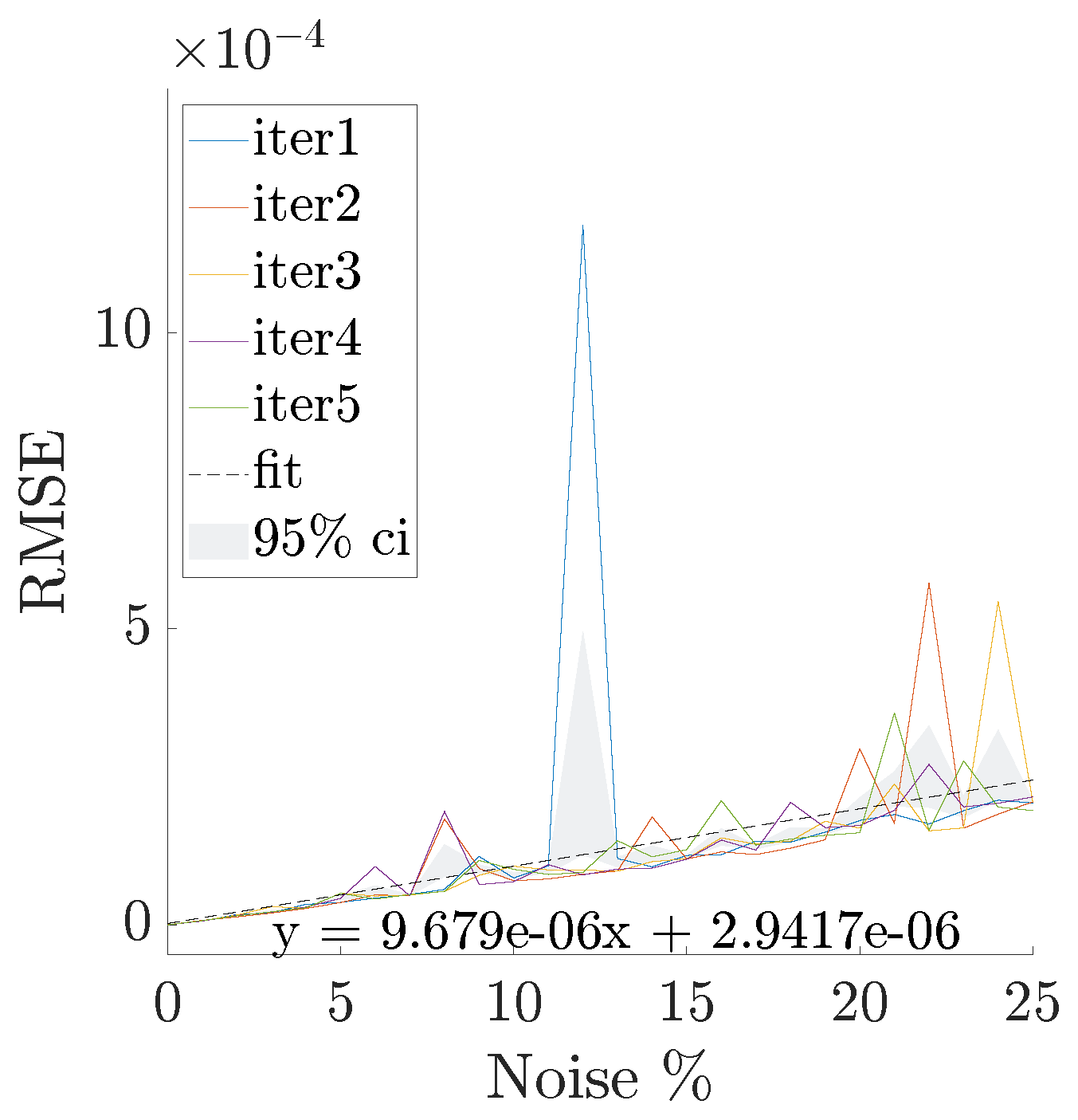
where I is the number of FRF columns and the other notation is consistent with Equation (5). The number of frequency points, K, is given by $f_s/2/\Delta f$, which returned 2000 points. The results on the goodness of fit of the model for the input–output 0, 1, and 5% noise are presented in Figure 3. Figure 4 shows the effect of noise, in all cases, for the correlation of ${\omega }_n$, ${\zeta }_n$ and ${\mathit{\varphi }}_n$. Figure 5 shows the effect of noise on the overall RMSE, mean of the RMSE over its samples, per given noise level and iteration.

Figure 3 shows the LF fit for three instances: clean (no noise), 1%, and 5% noise. The eight FRF channels, superimposed for conciseness, are shown by a red dashed line, the numerical data is represented by a blue line and the deviation is superimposed, for all channels, with a green line. The deviation is concerned with the magnitude of the FRF; however, phase fitness seems to be more severely affected by noise, particularly for high DoFs. While the difference between the noise-free and the noisy cases is noticeable, once AWGN is introduced, the deviation does not rise significantly with noise. Hence, it can be asserted, similar to what is found in [9], that phase modelling is more sensitive to noise than peak amplitude for the LF. Moreover, the deviation does not have a constant value, particularly referring to Figure 3b. In fact, a linear relation between deviation and frequency can be seen. This is explained by the nature of the LF because the sum of errors of the interpolation can grow with the frequency [9]. Hence, the relation can be justified by the sum of multiple interpolation errors along the FRF. In Figure 3b, the minimum order case $k=16$ (the minimum order is two times the number of discovered modes) is considered. This does not translate to poor identification of the modal parameters, because the order k of the LF is raised to identify stable poles.

Figure 4 compares the correlation between the numerical and estimated data when subjected to noise. Figure 4a–c show the input–output noise case. The main modal quantities, ${\omega }_n$, ${\zeta }_n$, and ${\mathit{\varphi }}_n$, are considered. ${\omega }_n$ and ${\zeta }_n$ estimation results are presented as the relative difference ($\Delta$), in percentage, calculated by:

$$\Delta =\frac{x_e-x_b}{x_b}\%$$

(7)

where $x_e$ and $x_b$ represent the estimated and baseline quantities, respectively. The increase in noise is inversely correlated with the precision of the modal parameter identification, as expected. The results for ${\omega }_n$ in Figure 4a show that a near-perfect identification is achieved for the noise-free scenario, and, as the noise level increases, the precision of the identification of the higher modes diminishes. The same is found in Figure 4b for ${\zeta }_n$ and, to a lesser extent, for ${\mathit{\varphi }}_n$ in Figure 4c. Nevertheless, the first mode is always correctly identified for all noise scenarios.

The effect of noise on the global RMSE is investigated in Figure 5. Five evaluations of the LF fit across the noise range are used for statistical significance and the corresponding 95% confidence interval (ci) is represented in the shaded area of Figure 5. A clear positive linear trend between noise and RSME is found, meaning that as noise increases, so too does the modelling error. For this study, the minimum order of k is used.

Notably, the global RMSE value never exceeds $8\times {10}^{-4}$ and Figure 4 shows that for small enough values of noise, the modal properties are correctly identified. This is confirmed in Figure 3 and Figure 5, where as the level of noise increases the fitted model deviates from the numerical data; however, this is particularly true for phase data rather than amplitude and modal parameters.

2.1.2. Investigation of the Structural Damage Effects

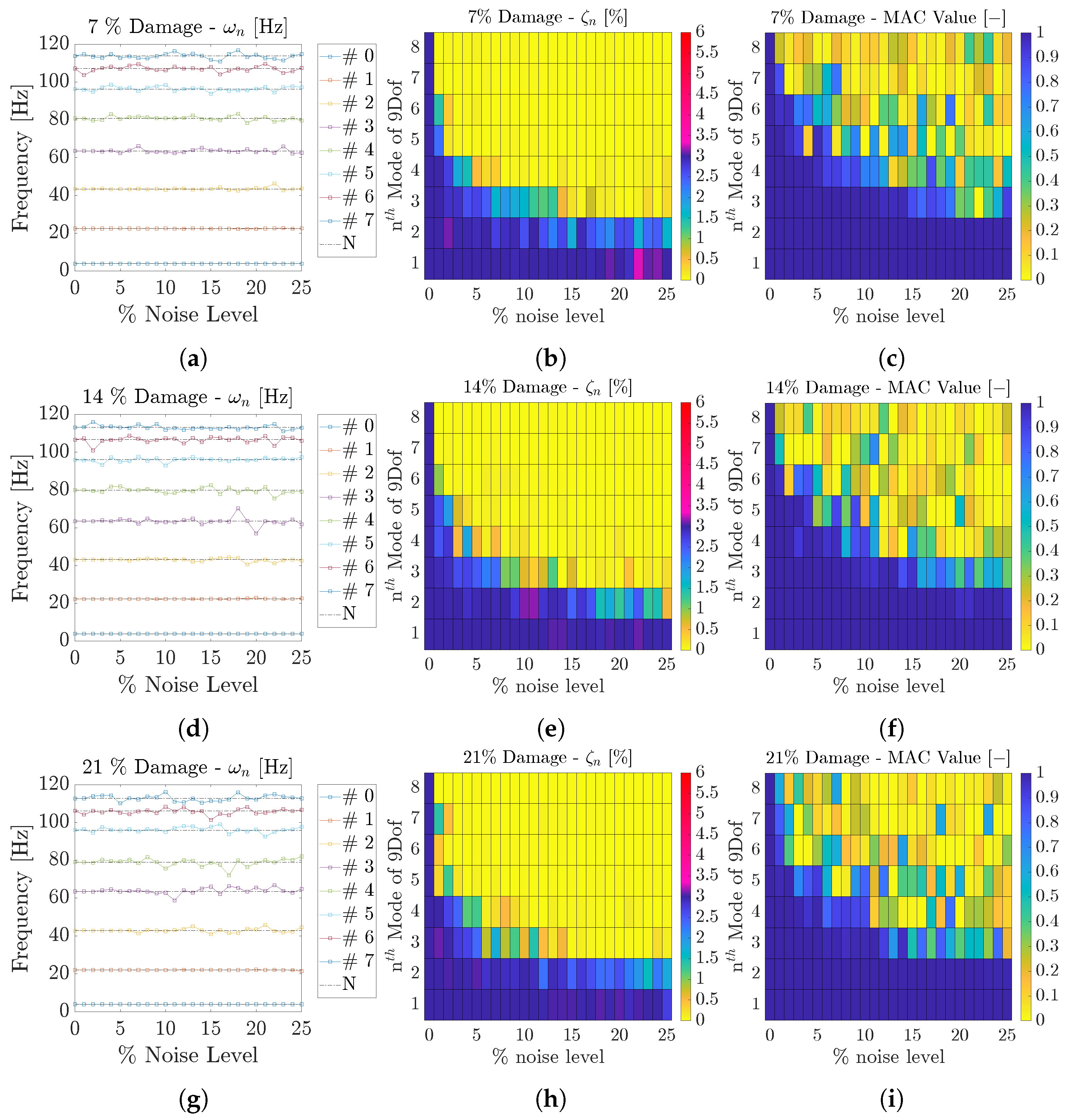
In order to further investigate the capabilities of the LF and foster the comparison with the experimental eight DoF system, three damaged numerical scenarios are introduced. Here, the suitability of the LF for SHM and its noise robustness is investigated. Three damaged scenarios, derived from the system presented in Figure 1, were built by reducing the stiffness of $k_5$ by 7, 14, and 21%. Only the stiffness was modified in these scenarios and ${\zeta }_n$ was left unchanged from the undamaged scenario, only used to evaluate the goodness of the identification. The same noise levels considered in the undamaged case were analysed for the damaged configurations. Hence, a total of 78 cases, 26 per scenario were considered. The results of the identifications via LF in this section are presented by comparing the modal parameters with those obtained numerically. For ${\omega }_n$ and ${\zeta }_n$, the numerical values are compared to those identified via LF. At the same time, for ${\mathit{\varphi }}_n$ the MAC value, from Equation (4), between the numerical and identified values is shown. The ${\omega }_n$ of the baseline and damaged numerical cases are shown in

Table 2. Eight DoF noise-free numerical system: natural frequencies, in Hz, of the numerical undamaged and damaged cases.

	Natural Frequency (Hz)
Mode #	Undamaged	7%	14%	21%
0	3.896	3.896	3.895	3.894
1	22.652	22.485	22.292	22.068
2	43.656	43.435	43.186	42.904
3	63.628	63.573	63.509	63.433
4	81.532	80.777	79.930	78.986
5	96.474	96.290	96.090	95.874
6	107.708	107.241	106.704	106.115
7	114.677	113.856	113.189	112.663

, serving as a source of comparison with the data in Figure 6.

For noise levels less than 1%, the LF is able to correctly identify all the parameters of the damaged cases, as shown in Figure 6. When the noise level was less than 5% the first five modes’ parameters were identified satisfactorily. In addition, the modal parameters of the first two modes are always coherent with the numerical counterpart for all noise levels. The hardest scenario for the LF identification was the 7% stiffness reduction scenario, where only a small change in modal parameters, see Table 2, is found, making it difficult to detect. Nevertheless, the LF is able to do so, hence demonstrating its capability for SHM.

In Figure 7 the ${\omega }_n$ and ${\mathit{\varphi }}_n$ of the first three modes of the undamaged and three damaged scenarios are compared for damage assessment. ${\zeta }_n$ is not considered as it was constant in all scenarios. Figure ${\mathit{\varphi }}_n$ shows the $\Delta$ (Equation (7)) change, with respect to the undamaged scenario, of the ${\omega }_{1-3}$ estimated by LF for the undamaged and damaged noiseless cases. In Figure 7b, the ${\mathit{\varphi }}_{1-3}$ of the undamaged and damaged scenario are compared for damage localisation. The differences between the ${\omega }_{1-3}$ increase linearly with the damage and the ${\mathit{\varphi }}_{1-3}$ trajectory deviation becomes more pronounced at the damaged fifth node. The combination of the ${\omega }_n$ and ${\mathit{\varphi }}_n$ results allows for damage assessment, ${\omega }_n$ and ${\mathit{\varphi }}_n$ (the higher the damage the more deviation), and localisation, ${\mathit{\varphi }}_n$, of the damage.

Given the results outlined in Figure 6 and Figure 7 and Table 2 and the above-mentioned discussion, the values of the LF for SHM and its robustness to noise is demonstrated. Specifically, these results are used in the following section to assess the model against the real experimental data.

2.2. Experimental System

In this section, the identification results of the experimental system in Figure 2 are presented. The LF results are compared to the well-established methods N4SID and LSCE. Two cases are taken into consideration, undamaged and damaged, 14 % stiffness reduction in the fifth element. These also allow for further comparison with the numerical system.

2.2.1. Undamaged Scenario

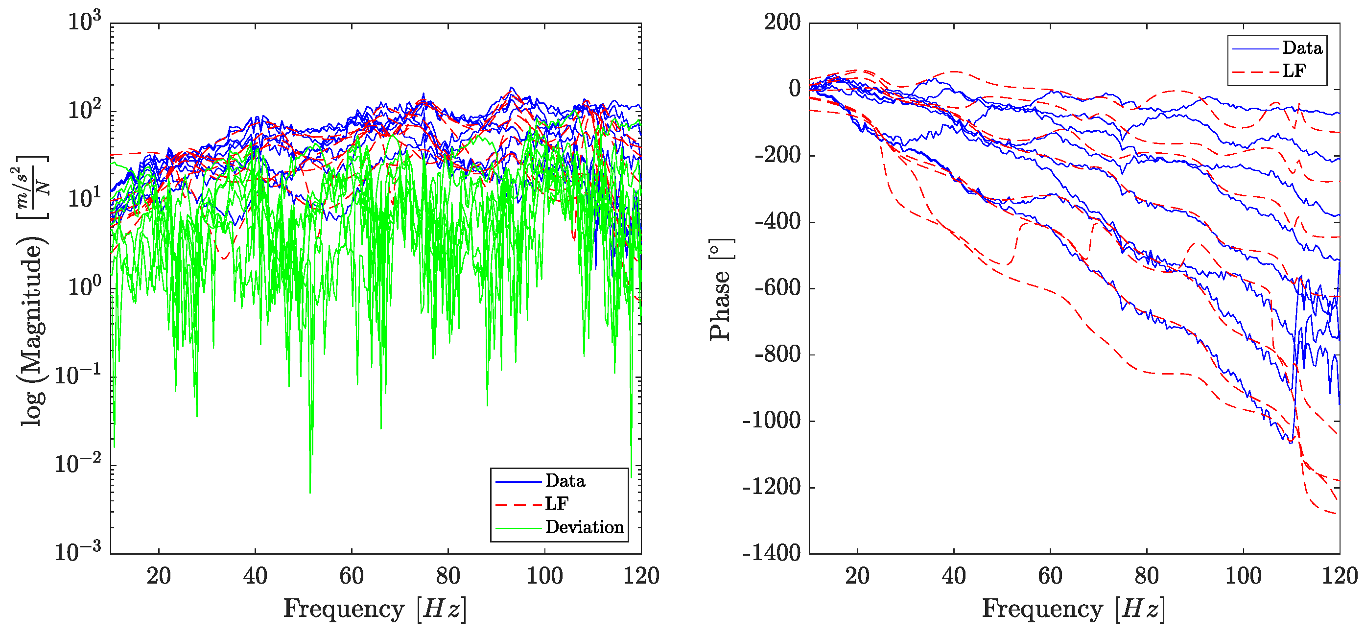
The analysis involved the goodness of fit of the LF, considering all channels in an SIMO fashion, to the computed acceleration FRF. Figure 8 shows the computed FRF as a solid blue line, the Loewner realisation as a dashed red line and the deviation, defined as the square of the difference’s absolute value at each frequency instance, with a solid green line. The plot on the left shows the absolute gain of the FRF, the LF fit, and the deviation, while the right plot shows the phase angle in degrees. In Figure 8, the FRF for this case is noisy and, as seen before, this mostly influences the higher frequencies and modes. The absolute gain plot shows, unequivocally, that the deviation trend increases with frequency. This phenomenon returns a coherent fit for the LF, except for the phase angle at higher frequencies, giving an absolute gain deviation between 10⁻² and 10². Nevertheless, this deviation magnitude still allows for a coherent identification of parameters by the LF, which is shown in

Table 3. Eight DOF experimental system (undamaged case): ${\omega }_n$, in Hz, and ${\zeta }_n$ identified by N4SID, LSCE, LF, LF from the noiseless numerical system (LF_num) and numerical system are compared to the benchmark results from [30]. The values in brackets refer to the relative difference between the estimated values and benchmark results. Only the first five modes were explicitly listed in [30].

	Natural Frequency (Hz)
Mode #	N4SID (%)	LSCE (%)	LF (%)	Benchmark	LF_num (%)	Numerical (%)
1	21.812	22.052	22.310	22.6	22.652	22.652
	(−3.49)	(−2.42)	(−1.28)		(0.23)	(0.23)
2	43.385	43.181	43.513	44.5	43.656	43.656
	(−2.51)	(−2.96)	(−2.22)		(−1.90)	(−1.90)
3	62.969	62.944	62.887	65.9	63.628	63.628
	(−4.45)	(−4.49)	(−4.57)		(1.18)	(1.18)
4	81.026	81.276	81.330	86.6	81.532	81.532
	(−6.44)	(−6.15)	(−6.09)		(−5.85)	(−5.85)
5	95.790	96.135	96.016	99.4	96.474	96.474
	(−3.63)	(−3.28)	(−3.40)		(−2.94)	(−2.94)
6	107.062	107.038	107.371	n.a.	107.708	107.708
	(n.a.)	(n.a.)	(n.a.)		(n.a.)	(n.a.)

,

Table 4. Eight DoF experimental system (undamaged case): ${\zeta }_n$ identified by N4SID, LSCE, LF, LF from the noiseless numerical system (LF_num) and numerical system are compared to the benchmark results from [30]. The values in brackets refer to the relative difference between the estimated values and benchmark results. Only the first five modes were explicitly listed in [30].

	Damping Ratio [-]
Mode #	N4SID (%)	LSCE (%)	LF (%)	Benchmark	LF_num (%)	Numerical (%)
1	0.084	0.093	0.084	0.085	0.030	0.030
	(−1.18)	(9.41)	(−1.18)		(−64.29)	(−64.29)
2	0.047	0.048	0.045	0.043	0.030	0.030
	(9.30)	(11.63)	(4.65)		(−30.23)	(−30.23)
3	0.039	0.036	0.028	0.033	0.030	0.030
	(18.18)	(9.09)	(−15.15)		(−9.10)	(−9.10)
4	0.030	0.029	0.027	0.050	0.030	0.030
	(−40.00)	(−42.00)	(−46.00)		(−40)	(−40)
5	0.026	0.021	0.022	0.026	0.030	0.030
	(0.00)	(−19.23)	(−15.38)		(15.38)	(15.38)
6	0.029	0.033	0.023	n.a.	0.030	0.030
	(n.a.)	(n.a.)	(n.a.)		(n.a.)	(n.a.)

and

Table 5. Eight DoF system (undamaged case): MAC matrix diagonal values between N4SID and LSCE, N4SID and LF, LF and LSCE, LF and LF_num and LF and the numerical system ${\varphi }_n$. The off-diagonal terms are negligible as they were all found to be close to zero, as expected.

	MAC Value (Main Diagonal Terms) (-)
Mode #	N4SID vs. LSCE	N4SID vs. LF	LF vs. LSCE	LF vs. LF_num	LF vs. Numerical
1	1	1	0.99	0.99	0.99
2	1	1	0.99	1	1
3	1	0.99	0.99	0.99	0.99
4	1	1	1	0.99	0.99
5	1	0.96	0.97	0.96	0.96
6	0.98	0.93	0.95	0.80	0.80

and Figure 9. It should be noted that the LF results in Figure 8 are obtained with the minimum order, in accordance with the literature results, of k= 12 (since only six modes were extracted in previous literature) and the modal parameters are obtained to the suitable higher-order as prescribed by the poles’ stability.

Table 3 and Table 4 introduce the raw values of the mean ($\mu$) over five iterations, taken for statistical significance, of the identified ${\omega }_n$, in Hz, and ${\zeta }_n$ by the LF and benchmark methods (LSCE and N4SID). Here, a quantitative comparison between N4SID, LSCE, LF, LF from the noiseless numerical system (LF_num), numerical system and benchmark data [30] is considered by showing, in brackets, their relative difference in percentage to the benchmark values. The ${\omega }_n$ identified within this work tend to be slightly underestimated when compared to the benchmark values. Nevertheless, the identified ${\omega }_{1-5}$ deviation from the expected benchmark values never exceeds 6.5%. The identified ${\zeta }_n$ are very coherent with the benchmark data. In fact, only ${\zeta }_4$ is noticeably underestimated (this is, however, in line with the estimations of the two other methodologies). In addition, LSCE notably overestimates ${\zeta }_1$. The same is valid for LF_num and the numerical system values. They are largely consistent with the N4SID and LF values for ${\omega }_n$. However, they present large discrepancies for ${\zeta }_n$, since that parameter is assumed to be 3% for all modes in the original model.

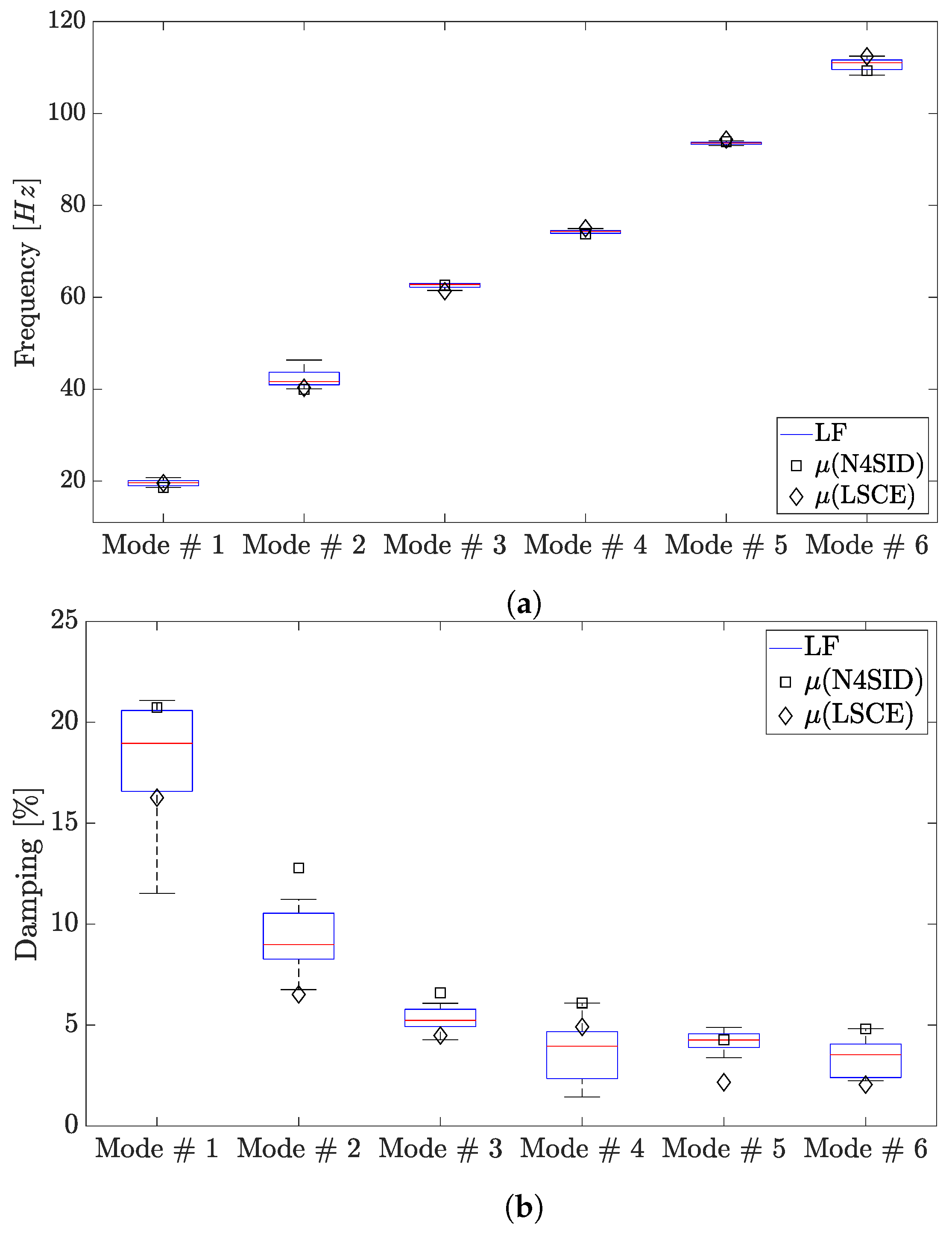
Figure 9 shows the statistical performance of the LF against the mean of the established methods. The choice of presenting the established methods through their mean and not according to the LF is based on the nature of their standard deviation ($\sigma$), which is of a negligible magnitude if compared with the LF’s own, and to maintain clarity within the plot. Overall, Figure 9 shows that the LF-identified ${\omega }_n$ and ${\zeta }_n$ are in line with the values found through LSCE and N4SID identification.

The first six ${\mathit{\varphi }}_{1-6}$ of the eight DoF system are compared in Table 5 using the MAC value. The LF slightly underperforms identifying the sixth mode of the undamaged case. Nevertheless, the sixth mode shape is still consistent with the ones identified by LSCE and N4SID. The MAC values between the sixth mode identified by the LF, LSCE, and N4SID are 0.95 and 0.93, respectively. Hence, this is well above what is commonly considered a sufficient correlation by practitioners [35,37]. In summary, the first six modes of the eight DoF system are identified by LF accordingly to N4SID and LSCE. The numerical model and LF_num perform well for the first five modes (MAC values are above 0.96); however, they fall short at the sixth mode with an MAC value of 0.80. Notably, this is also the mode for which the quantitative benchmark values are not available [30].

As well as the accuracy and precision, the efficiency of the method is evaluated. The approach taken here considers the $\mu$ and $\sigma$ of the time elapsed till identification on the experimental data over several iterations (five in this case), at the order k. The results are satisfactory when compared with well-established methods. The results are presented in

Table 6. Eight DoF experimental system (undamaged case): Time elapsed till identification (over five instances for statistical significance), in s, for N4SID, LSCE, and LF of the undamaged case. k represents the model order.

	Time to Identification (s)
	N4SID	LSCE	LF
$\mu$	16.626	0.010	0.199
$\sigma$	±0.172	± <0.001	±0.006
k	25	30	50

, in which LSCE is recognised as the least computationally demanding method and N4SID as the most. The LF lies between them, both in terms of $\mu$ and $\sigma$. The values presented in Table 6 were computed in MATLAB R2022b running on a desktop Microsoft Windows 11 machine with a 6-core AMD Ryzen 5 5600G.

2.2.2. Damaged Scenario

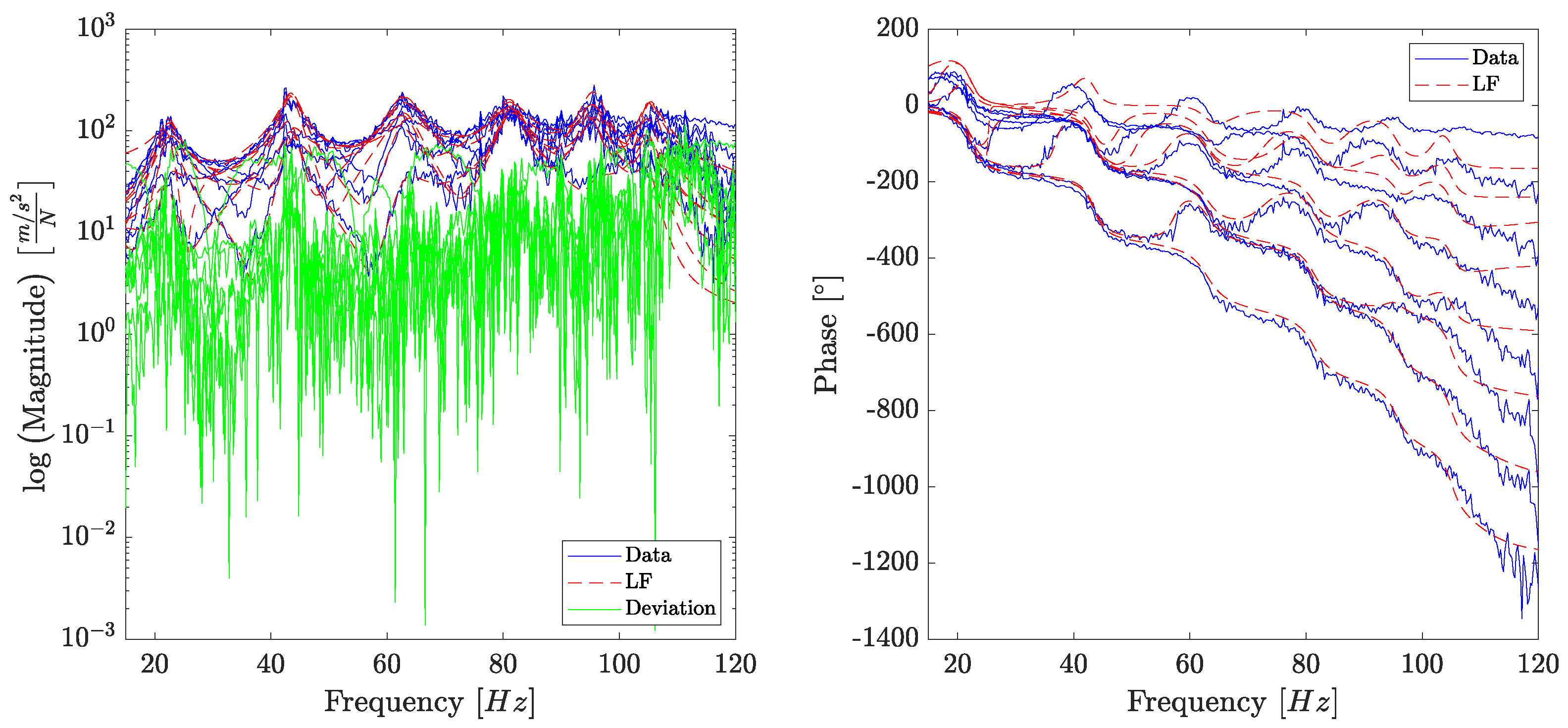
The damaged case is characterised by a 14% reduction in the stiffness of the fifth element. As for the undamaged case, the results obtained from N4SID, LSCE, LF, LF_num and the numerical system are compared to the benchmark values with respect to the identified parameters. The FRF for the damaged system is even noisier than the undamaged, as shown in Figure 10. The deviation between the acceleration FRF and the Loewner realisation is between 10⁻² and 10². Nevertheless, the LF model holds a reasonable approximation for the experimental FRF, particularly for the gain amplitude.

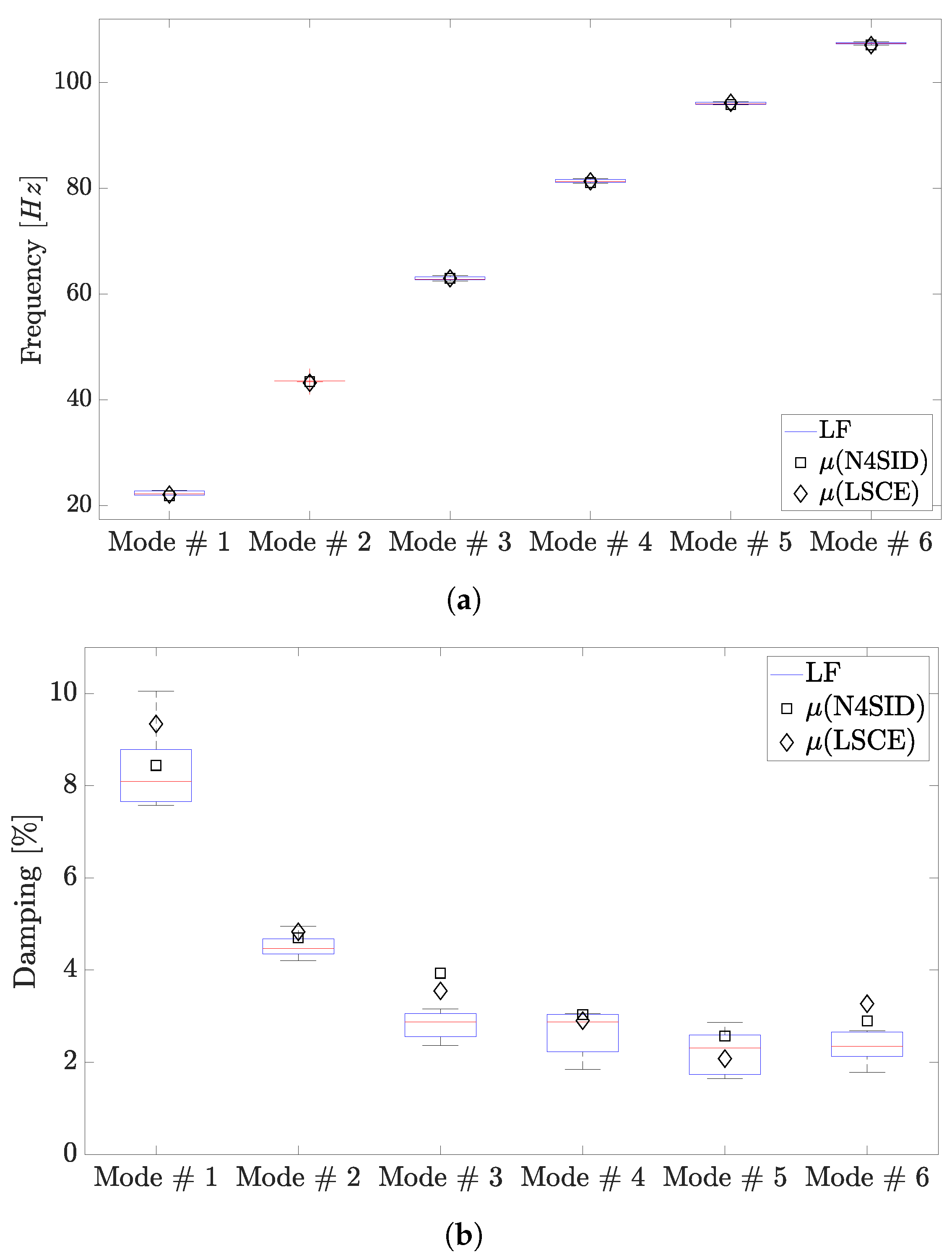
${\omega }_n$ benchmark values are available from [30], while they are not for ${\zeta }_n$ and ${\mathit{\varphi }}_n$. Hence, N4SID-identified values, the mean over five realisations, are used as the baseline for their comparisons.

Table 7. Eight DOF experimental system (damaged case): ${\omega }_n$, in Hz, and ${\zeta }_n$ identified by N4SID, LSCE, LF, LF from the noiseless numerical system (LF_num) and numerical system are compared to the benchmark results from [30]. The values in brackets refer to the relative difference between the estimated values and the benchmark results. Only the first five modes were explicitly listed in [30].

	Natural Frequency (Hz)
Mode #	N4SID (%)	LSCE (%)	LF (%)	Benchmark	LF_num (%)	Numerical (%)
1	18.636	19.567	19.608	22.3	22.292	22.292
	(−16.43)	(−12.26)	(−12.07)		(0.04)	(0.04)
2	39.983	40.308	42.422	43.9	43.186	43.186
	(−8.92)	(−8.18)	(−3.367)		(−1.63)	(−1.63)
3	62.643	61.326	62.561	64.8	63.510	63.510
	(−3.33)	(−5.36)	(−3.46)		(1.99)	(1.99)
4	73.741	75.014	74.297	85.9	79.930	79.930
	(−6.44)	(−6.15)	(−6.09)		(−5.85)	(−5.85)
5	93.843	94.315	93.518	99.7	96.090	96.090
	(−3.63)	(−3.28)	(−3.40)		(−2.94)	(−2.94)
6	109.288	112.412	110.627	n.a.	106.704	106.704
	(n.a.)	(n.a.)	(n.a.)		(n.a.)	(n.a.)

shows the comparison for ${\omega }_n$. ${\zeta }_n$ results are shown in

Table 8. Eight DoF experimental system (damaged case): ${\zeta }_n$ identified by N4SID, LSCE, LF, LF from the noiseless numerical system (LF_num) and numerical system are shown. The values in brackets refer to the relative difference between the estimated values and the N4SID values.

	Damping Ratio (-)
Mode #	N4SID (%)	LSCE (%)	LF (%)	LF_num (%)	Numerical (%)
1	0.207	0.163	0.181	0.030	0.030
		(−21.26)	(−12.56)	(−85.51)	(−85.51)
2	0.128	0.065	0.092	0.030	0.030
		(−49.22)	(28.13)	(−76.56)	(−76.56)
3	0.066	0.045	0.053	0.030	0.030
		(−31.81)	(−19.70)	(−54.54)	(−54.54)
4	0.061	0.049	0.037 0.030	0.030
		(−19.67)	(−39.34)	(−50.82)	(−50.82)
5	0.043	0.022	0.042	0.030	0.030
		(−48.84)	(−2.33)	(−30.23)	(−30.23)
6	0.048	0.021	0.034	0.030	0.030
		(−56.25)	(−29.17)	(−37.50)	(−37.50)

and the ${\mathit{\varphi }}_n$ are compared to the N4SID values computing the MAC in

Table 9. Eight DoF system (damaged case): MAC matrix diagonal values between N4SID and LSCE, N4SID and LF, LF and LSCE, LF and LF_num and LF and the numerical system ${\varphi }_n$. The off-diagonal terms are negligible as they are close to zero.

	MAC Value (Main Diagonal Terms (-)
Mode #	N4SID vs. LSCE	N4SID vs. LF	LF vs. LSCE	LF vs. LF_num	LF vs. Numerical
1	0.99	0.97	0.97	0.99	0.99
2	0.96	0.99	0.93	1	1
3	0.98	0.99	0.97	0.99	0.99
4	0.98	0.99	1	0.99	0.99
5	0.99	0.98	0.98	0.96	0.96
6	0.89	0.93	0.86	0.80	0.80

. Figure 11 gives a more intuitive representation of the range of ${\omega }_n$ and ${\zeta }_n$ identified via LF, LSCE, and N4SID.

In Table 7, the ${\omega }_n$ identified by N4SID, LSCE, LF and LF_num and those obtained from the numerical system are compared, while in Figure 11a the identified ${\omega }_n$ via LF over five realisations are compared to the average values from LF and LSCE. When compared to the benchmark values, ${\omega }_1$ seems severely underestimated (over 10 %) by N4SID, LSCE, and LF, while those based on the numerical system performed very well (error close to zero). However, while the input type is mentioned in [30], the same cannot be said for its amplitude. In fact, it is not clear which, of the three available, is used to obtain the benchmark results (3 V RMS is used in this work). This would be decisive in determining if the discrepancy is an error or a result of the amplitude-dependent non-linearity of the system. This said, the maximum error for the remaining modes never exceeds 9% for N4SID, 8.20% for LSCE, 6.1% for LF and 5.9% for LF_num and the numerical system. Concerning ${\zeta }_n$, the identification becomes more spurious, as expected given the noisy experimental FRF, shown in Figure 10. Nevertheless, the ${\zeta }_n$ are underestimated for all modes by LF and LSCE, when compared to N4SID. However, this is even more true for LSCE, for which the ${\zeta }_n$ of all modes are greatly underestimated. LSCE outperforms LF only for the identification of ${\zeta }_4$. Generally, it can be said that LF and, more relevantly, LSCE have slightly underestimated ${\zeta }_n$. These are clearly shown in Table 8 and Figure 11b.

With respect to ${\mathit{\varphi }}_n$, benchmark values are not disclosed, as per the undamaged case, in [30]. Hence, N4SID data are used as a reference for the comparison in Table 9, where the MAC values are used as a figure of merit. Notably, ${\mathit{\varphi }}_n$ identified via LF show a higher correlation to the N4SID ${\mathit{\varphi }}_n$ than those identified by LSCE, apart from ${\mathit{\varphi }}_4$. Nevertheless, the LF-identified ${\mathit{\varphi }}_n$ MAC values with respect to N4SID are, for all modes, at least 0.93. A correlation is also seenn between the LF_num and numerical modes with LF.

As per the undamaged scenario in Table 6, the time till identification for the LF, LSCE, and N4SID on the experimental data is investigated for the damaged case as well. In

Table 10. 8 DoF experimental system (damaged case): Time to identification (over five instances for statistical significance), in s, for N4SID, LSCE, and LF of the damaged case. k represents the model order.

	Time to Identification (s)
	N4SID	LSCE	LF
$\mu$	37.012	0.013	0.216
$\sigma$	±0.075	±0.001	±0.007
k	30	34	80

, the results in terms of $\mu$ and $\sigma$ of the time till identification, in seconds, and their order k are presented. The same picture as per Table 6 emerged. The only difference is the magnitude of the time till identification, which is higher due to a higher order k necessary to obtain significant results.

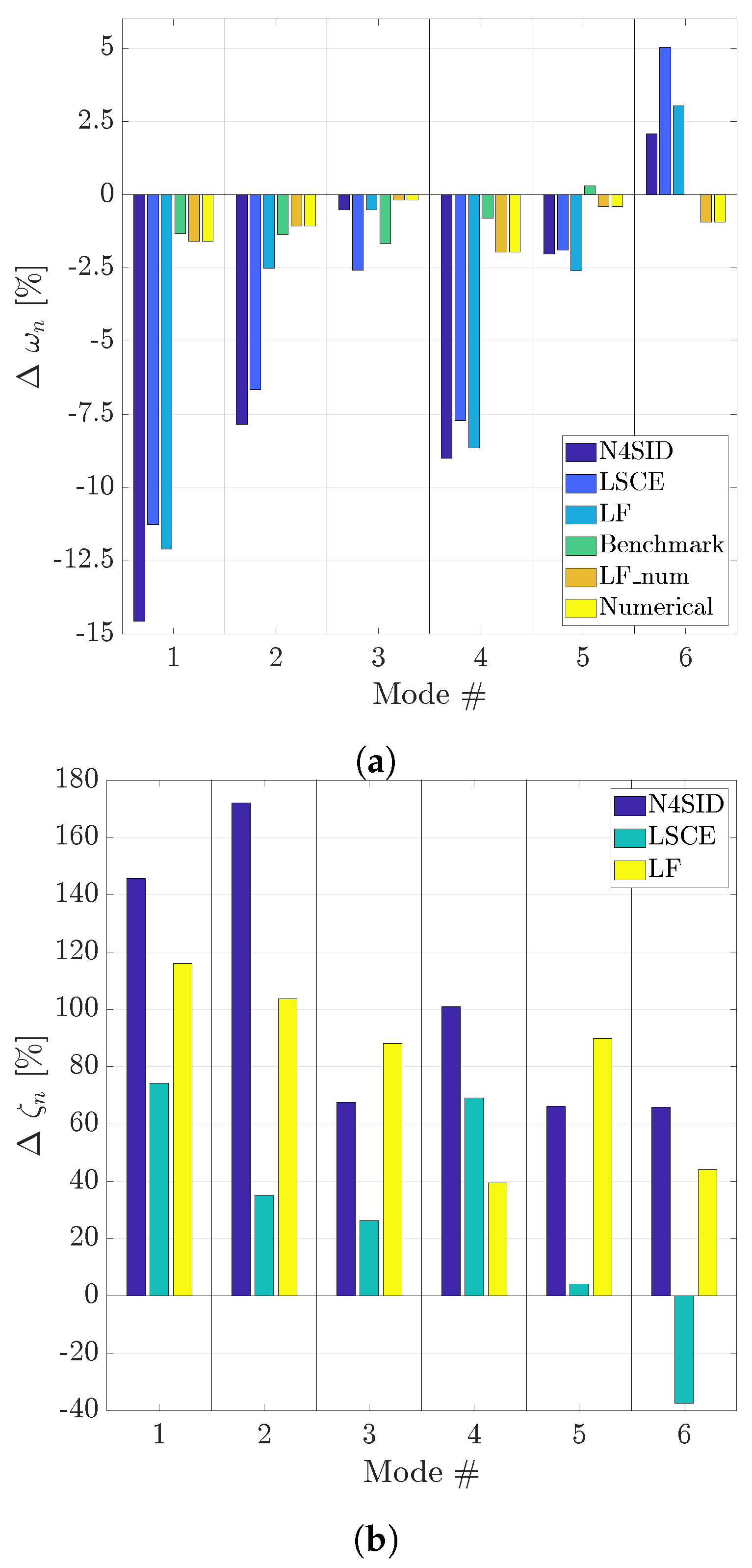
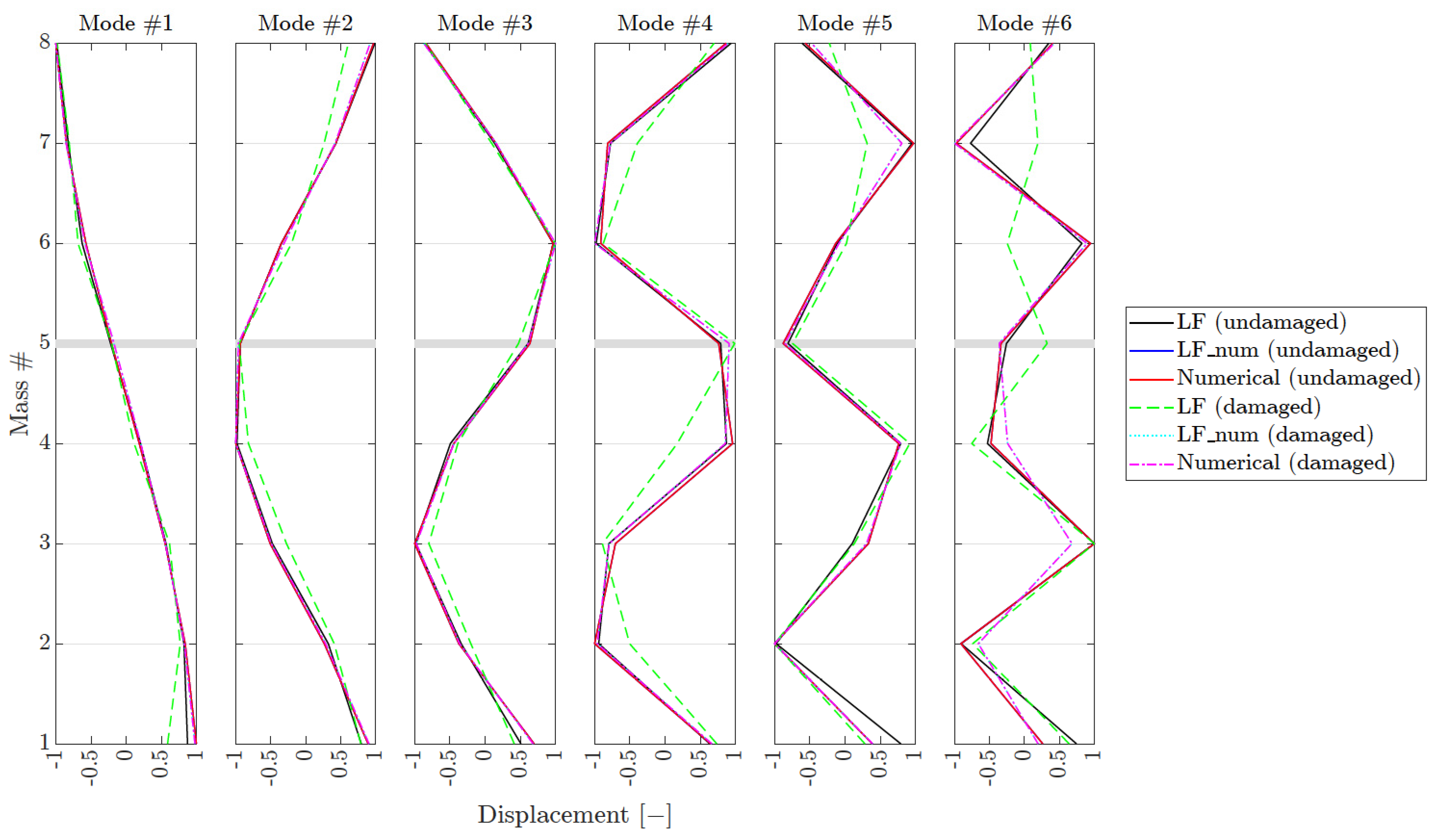
Having established the goodness of the LF identification, when compared to benchmark data and N4SID, it is necessary to carry out a damage assessment on the structure. As is noted in [25], the expectation for a stiffness reduction is a decrease in ${\omega }_n$ and a change in the ${\mathit{\varphi }}_n$ trajectories, particularly at the damaged node. In Figure 12, the relative difference between the undamaged and damaged cases ${\omega }_n$ (Figure 12a) and ${\zeta }_n$ (Figure 12b) are presented. The comparison for ${\omega }_n$ includes results from N4SID, LSCE, LF, benchmark, LF_num and the numerical system, while for ${\zeta }_n$ only from N4SID, LSCE and LF, since benchmark values are not available for ${\zeta }_n$ and it is constant at 3% for the data relative to the numerical system (no change between damaged and undamaged). The undamaged and damaged ${\mathit{\varphi }}_n$ identified from the experimental data by LF, LF_numand the numerical system are shown in Figure 13.

In Figure 12a, a negative relative difference is found for all methods and modes, apart from ${\omega }_5$ for the benchmark values and ${\omega }_6$ for the methods that use experimental data. This allows the detection of a change in the structural behaviour, thus detecting damage [25]. It should be noted that the experimental methods see a larger relative difference between damaged and undamaged ${\omega }_n$ than the benchmark and model-based methods. However, uncertainty on the origin of the benchmark data, particularly concerning the input amplitude (as already pointed out) and processing of the data, remains. Nevertheless, LF performs coherently to the other experimental methods, and LF_num results are perfectly correlated to the numerical results. Hence, the difference is not due to the method but the data or system under scrutiny.

On the other hand, for ${\zeta }_n$, an increase is registered for all modes and methods, apart from ${\zeta }_6$ for LSCE. An increase in damping is usually seen as a damage indicator [25]; however, since it is easily influenced by external factors [17] it is rarely used as such. Notably, the LF increase in ${\zeta }_n$ is always closer to N4SID than LSCE, apart for ${\zeta }_{4-5}$.

Figure 13 compares the damaged and undamaged ${\mathit{\varphi }}_n$ and successfully demonstrates the ability of the LF to detect differences, which is a preparation step for damage localisation [25]. Notably, ${\mathit{\varphi }}_{1-5}$ are largely consistent across all methods, proving the goodness of the LF as a modal parameter identification method for SHM.

In essence and given the above-mentioned results, the LF is an effective SI method for SHM in mechanical systems as it was able to detect parameter difference between the damaged and undamaged systems in a similar or improved manner than well-established methods, benchmark values, and numerical models.

3. Conclusions

In this study, the precision, robustness, and computational efficiency of the LF were assessed for the identification of the modal parameters of an eight DoF numerical and experimental dataset from the EI at the LANL. Damage detection, considering severity and localisation, was considered by interpreting the changes in modal parameters between the baseline and damaged states, while robustness was investigated by corrupting the numerical signals with additive Gaussian white noise at different levels.

In the numerical model, the LF performance was compared to the numerical results, while in the experimental study two industry-standard system identification methods, N4SID and LSCE, and known benchmark results were used to assess the LF performance. Good agreement was found between the modal parameters estimated via the LF and those identified via N4SID and LSCE. In particular, it can generally be said that LF was more precise in the identification of natural frequencies and damping ratios than LSCE and its accuracy and precision are on par with N4SID.

The noise robustness of the LF was verified on the numerical dataset, showing that the LF can accurately identify all modes at low noise levels and lower modes at higher noise levels.

Regarding the identification time (considering an average over five realisations), LSCE was the fastest method and N4SID was the slowest. The LF ran at an order of magnitude slower than LSCE but two orders of magnitude faster than N4SID.

Given the results and conclusions presented, the authors suggest the use of the LF over N4SID for its improved computational efficiency and over LSCE for its damping ratio identification capability.

References

1. Ljung, L. System Identification: Theory for the User, 1st ed.; Prentice Hall: Englewood Cliffs, NJ, USA, 1987. [Google Scholar]
2. Mugnaini, V.; Zanotti Fragonara, L.; Civera, M. A machine learning approach for automatic operational modal analysis. Mech. Syst. Signal Process. 2022, 170, 108813. [Google Scholar] [CrossRef]
3. Dessena, G.; Ignatyev, D.I.; Whidborne, J.F.; Pontillo, A.; Zanotti Fragonara, L. Ground vibration testing of a high aspect ratio wing with revolving clamp. In Proceedings of the 33rd Congress of the International Council of the Aeronautical Sciences, Stockholm, Sweden, 4–9 September 2022. [Google Scholar] [CrossRef]
4. Dessena, G.; Ignatyev, D.I.; Whidborne, J.F.; Pontillo, A.; Zanotti Fragonara, L. Ground vibration testing of a flexible wing: A benchmark and case study. Aerospace 2022, 9, 438. [Google Scholar] [CrossRef]
5. Civera, M.; Calamai, G.; Zanotti Fragonara, L. System identification via fast relaxed vector fitting for the structural health monitoring of masonry bridges. Structures 2021, 30, 277–293. [Google Scholar] [CrossRef]
6. Boscato, G.; Russo, S.; Ceravolo, R.; Fragonara, L.Z. Global sensitivity-based model updating for heritage structures. Comput.-Aided Civ. Infrastruct. Eng. 2015, 30, 620–635. [Google Scholar] [CrossRef]
7. Dessena, G.; Ignatyev, D.I.; Whidborne, J.F.; Zanotti Fragonara, L. A Kriging Approach to Model Updating for Damage Detection. In EWSHM 2022, LNCE 254 ed.; Rizzo, P., Milazzo, A., Eds.; Springer: Singapore, 2023; Chapter 26; pp. 245–255. [Google Scholar] [CrossRef]
8. Mayo, A.J.; Antoulas, A.C. A framework for the solution of the generalized realization problem. Linear Algebra Its Appl. 2007, 425, 634–662. [Google Scholar] [CrossRef] [Green Version]
9. Dessena, G.; Civera, M.; Zanotti Fragonara, L.; Ignatyev, D.I.; Whidborne, J.F. A Loewner-Based system identification and structural health monitoring approach for mechanical systems. Struct. Control Health Monit. 2023, 2023, 1–22. [Google Scholar] [CrossRef]
10. Gosea, I.V.; Antoulas, A.C. Model reduction of linear and nonlinear systems in the Loewner framework: A summary. In Proceedings of the 2015 European Control Conference (ECC), Linz, Austria, 15–17 July 2015; pp. 345–349. [Google Scholar] [CrossRef]
11. Löwner, K. Uber monotone matrixfunktionen. Math. Z. 1934, 38, 177–216. [Google Scholar] [CrossRef]
12. Civera, M.; Mugnaini, V.; Zanotti Fragonara, L. Machine learning-based automatic operational modal analysis: A structural health monitoring application to masonry arch bridges. Struct. Control. Health Monit. 2022, 29, e3028. [Google Scholar] [CrossRef]
13. Kramer, B.; Gugercin, S. Tangential interpolation-based eigensystem realization algorithm for MIMO systems. Math. Comput. Model. Dyn. Syst. 2016, 22, 282–306. [Google Scholar] [CrossRef]
14. Lefteriu, S.; Antoulas, A.C. Modeling multi-port systems from frequency response data via tangential interpolation. In Proceedings of the 2009 IEEE Workshop on Signal Propagation on Interconnects, Strasbourg, France, 12–15 May 2009; pp. 1–4. [Google Scholar] [CrossRef]
15. Lefteriu, S.; Antoulas, A.C. A new approach to modeling multiport systems from frequency-domain data. IEEE Trans. Comput.-Aided Des. Integr. Circuits Syst. 2010, 29, 14–27. [Google Scholar] [CrossRef]
16. Antoulas, A.C.; Lefteriu, S.; Ionita, A.C. A Tutorial Introduction to the Loewner Framework for Model Reduction. In Model Reduction and Approximation; Number May 2011; Society for Industrial and Applied Mathematics: Philadelphia, PA, USA, 2017; Chapter 8; pp. 335–376. [Google Scholar] [CrossRef]
17. Civera, M.; Calamai, G.; Zanotti Fragonara, L. Experimental modal analysis of structural systems by using the fast relaxed vector fitting method. Struct. Control Health Monit. 2021, 28, e2695. [Google Scholar] [CrossRef]
18. Dessena, G.; Civera, M.; Pontillo, A.; Ignatyev, D.I.; Whidborne, J.F.; Zanotti Fragonara, L. Novel Modal Parameters Extraction Methods for Aeronautical Structures. School of Aerospace, Transport and Manufacturing, Cranfield University: Cranfield, Bedforshire, UK, 2023; in preparation. [Google Scholar]
19. Dessena, G. A tutorial on the Loewner-based system identification and structural health monitoring approach for mechanical systems. Comput. Program 2022, 2023. [Google Scholar] [CrossRef]
20. Farrar, C.R.; Doebling, S.W.; Nix, D.A. Vibration–based structural damage identification. Philos. Trans. R. Soc. London. Ser. A Math. Phys. Eng. Sci. 2001, 359, 131–149. [Google Scholar] [CrossRef]
21. Gelman, L.; Petrunin, I.; Parrish, C.; Walters, M. Novel health monitoring technology for in-service diagnostics of intake separation in aircraft engines. Struct. Control Health Monit. 2020, 27, e2479. [Google Scholar] [CrossRef] [Green Version]
22. Zanotti Fragonara, L.; Boscato, G.; Ceravolo, R.; Russo, S.; Ientile, S.; Pecorelli, M.L.; Quattrone, A. Dynamic investigation on the Mirandola bell tower in post-earthquake scenarios. Bull. Earthq. Eng. 2017, 15, 313–337. [Google Scholar] [CrossRef] [Green Version]
23. Civera, M.; Fragonara, L.Z.; Surace, C. Nonlinear dynamics of cracked, cantilevered beam-like structures undergoing large deflections. In Proceedings of the 2019 IEEE 5th International Workshop on Metrology for AeroSpace (MetroAeroSpace), Turin, Italy, 19–21 June 2019; pp. 193–202. [Google Scholar] [CrossRef]
24. Cancelli, A.; Laflamme, S.; Alipour, A.; Sritharan, S.; Ubertini, F. Vibration-based damage localization and quantification in a pretensioned concrete girder using stochastic subspace identification and particle swarm model updating. Struct. Health Monit. 2020, 19, 587–605. [Google Scholar] [CrossRef]
25. Rytter, A. Vibrational Based Inspection of Civil Engineering Structures. Ph.D. Thesis, Aalborg University, Aalborg, Denmark, 1993. [Google Scholar]
26. Sohn, H.; Farrar, C.R.; Hemez, F.; Czarnecki, J.; Shunk, D.D.; Stinemates, D.W.; Nadler, B.R.; Czarnecki, J. A Review of Structural Health Monitoring Literature: 1996–2001; Technical report; Los Alamos National Laboratory (LANL): Los Alamos, CA, USA, 2004. [Google Scholar]
27. Cawley, P. Structural health monitoring: Closing the gap between research and industrial deployment. Struct. Health Monit. 2018, 17, 1225–1244. [Google Scholar] [CrossRef] [Green Version]
28. Van Overschee, P.; De Moor, B. N4SID: Subspace algorithms for the identification of combined deterministic-stochastic systems. Automatica 1994, 30, 75–93. [Google Scholar] [CrossRef]
29. Brown, D.L.; Allemang, R.J.; Zimmerman, R.; Mergeay, M. Parameter Estimation Techniques for Modal Analysis; SAE Transactions: Warrendale, PA, USA, 1979; Volume 790221, p. 19. [Google Scholar] [CrossRef]
30. Hemez, F.M.; Doebling, S.W. Review and assessment of model updating for non-linear, transient dynamics. Mech. Syst. Signal Process. 2001, 15, 45–74. [Google Scholar] [CrossRef]
31. Hemez, F.; Doebling, S. Validation of structural dynamics models at Los Alamos National Laboratory. In Proceedings of the 41st Structures, Structural Dynamics, and Materials Conference and Exhibit, Reston, VA, USA, 3–6 April 2000; American Institute of Aeronautics and Astronautics: Reston, VA, USA, 2000; pp. 1–8. [Google Scholar] [CrossRef] [Green Version]
32. Sohn, H.; Farrar, C.R. Damage diagnosis using time series analysis of vibration signals. Smart Mater. Struct. 2001, 10, 446–451. [Google Scholar] [CrossRef] [Green Version]
33. Bull, L.A.; Gardner, P.A.; Gosliga, J.; Rogers, T.J.; Dervilis, N.; Cross, E.J.; Papatheou, E.; Maguire, A.E.; Campos, C.; Worden, K. Foundations of population-based SHM, Part I: Homogeneous populations and forms. Mech. Syst. Signal Process. 2021, 148, 107141. [Google Scholar] [CrossRef]
34. Figueiredo, E.; Park, G.; Figueiras, J.; Farrar, C.; Worden, K. Structural Health Monitoring Algorithm Comparisons Using Standard Data Sets; Technical Report; Los Alamos National Laboratory (LANL): Los Alamos, NM, USA, 2009. [Google Scholar] [CrossRef] [Green Version]
35. Ewins, D.J. Modal Testing Theory, Practice and Application, 2nd ed.; Research Studies Press: Baldock, UK, 2000; p. 562. [Google Scholar]
36. Allemang, R.J.; Brown, D.L. A correlation coefficient for modal vector analysis. In Proceedings of the 1st International Modal Analysis Conference, Orlando, FL, USA, 8–10 November 1982; Union Coll: Orlando, FL, USA, 1982; pp. 110–116. [Google Scholar]
37. Ewins, D.J. Model validation: Correlation for updating. Sadhana 2000, 25, 221–234. [Google Scholar] [CrossRef]
Figure 1. Eight DoF numerical system: schematic diagram (adapted from [33]).
Aerospace 10 00571 g001
Figure 2. LANL eight DoF system (retrieved from [32]).
Aerospace 10 00571 g002
Figure 3. Eight DoF numerical system: the eight DoF system numerical recipient FRF is compared with LF’s transfer function results for the 0% (a), 1% (b), and 5% (c) input–output noise cases. In each sub-figure, from left to right, the gain’s absolute value and the phase angle are presented, for conciseness all eight channels are superimposed.
Aerospace 10 00571 g003
Figure 4. Eight DoF numerical system: In (ac) the effect of the output–input noise is investigated. The first column refers to the relative difference in ω n , in %, corresponding to the numerical results. Likewise, the second column refers to the ζ n , while the third column reports on the MAC value between the numerical and estimated values of ϕ n .
Aerospace 10 00571 g004
Figure 5. Eight DoF numerical system: Results of the numerical study and the relationshipbetween the noise level and global RMSE. The term 95% ci stands for 95% confidence interval.
Aerospace 10 00571 g005
Figure 6. Eight DoF numerical system: 7% damage (top), 14% damage (middle), 21% damage (bottom). Results of the numerical study on the numerical case effected by input–output noise: (a,d,g) The effect on ω n identification; (b,e,h) the effect on ζ n ; (c,f,i) the effect on ϕ n . In the legend, A stands for the numerical results and # n stands for Mode # n.
Aerospace 10 00571 g006
Figure 7. Eight DoF numerical system: Relative difference, in percentage, between baseline and damaged cases in ω n for the first three modes (a) and the first three ϕ n for the numerical baseline and damaged cases (b). The data refers to the noiseless case identified by LF and the thicker grid line marks the damage location.
Aerospace 10 00571 g007
Figure 8. Eight DoF experimental system (undamaged case): The FRF computed from the test data is compared with the LF’s transfer function for the undamaged case. The absolute gain (left) and phase angle (right) are presented with all eight channels superimposed for conciseness.
Aerospace 10 00571 g008
Figure 9. Eight DoF experimental system (undamaged case): Box plot of the ω n (a) and ζ n (b) for each mode of the undamaged case. The median value is represented by the central red line. The bottom and top blue edges of the box indicate the 25% and 75% percentiles. The whiskers represent the largest and smallest data points not considered outliers. The red plus symbol indicates the outlier values. The diamond represents the mean values (over five iterations) identified via LSCE and the square via N4SID.
Aerospace 10 00571 g009
Figure 10. Eight DoF experimental system (damaged case): The FRF computed from the test data is compared with the LF’s transfer function for the damaged case. The absolute gain (left) and the phase angle (right) are presented with all eight channels superimposed for conciseness.
Aerospace 10 00571 g010
Figure 11. Eight DoF experimental system (damaged case): Box plot of the ω n (a) and ζ n (b) for each mode of the damaged case. The median value is represented by the central red line. The bottom and top blue edges of the box indicate the 25% and 75% percentiles. The whiskers represent the largest and smallest data points not considered outliers. The red plus symbol indicates the outlier values. The diamond represents the mean values (over five iterations) identified via LSCE and the square via N4SID.
Aerospace 10 00571 g011
Figure 12. Eight DoF system: Comparison of the ω n (a) and ζ n (b) relative differences between the undamaged and damaged cases. For ω n , results from N4SID, LSCE, LF, benchmark, LF_num and the numerical system are presented, while for ζ n results from N4SID, LSCE and LF are presented.
Aerospace 10 00571 g012
Figure 13. Eight DoF system: Mode shapes of the first six modes, from the experimental data by LF, the LF_num system and the numerical system for the undamaged and damaged cases are plotted herein. The thicker grid line mark the damage location.
Aerospace 10 00571 g013