Compressor Performance Prediction Based on the Interpolation Method and Support Vector Machine

Abstract

Compressors are important components in various power systems in the field of energy and power. In practical applications, compressors often operate under non-design conditions. Therefore, accurate calculation on performance under various operating conditions is of great significance for the development and application of certain power systems equipped with compressors. To calculate and predict the performance of a compressor under all operating conditions through limited data, the interpolation method was combined with a support vector machine (SVM). Based on the known data points of compressor design conditions, the interpolation method was adopted to obtain training samples of the SVM. In the calculation process, preliminary screening was conducted on the kernel functions of the SVM. Two interpolation methods, including linear interpolation and cubic spline interpolation, were used to obtain sample data. In the subsequent training process of the SVM, the genetic algorithm (GA) was used to optimize its parameters. After training, the available data were compared with the predicted data of the SVM. The results show that the SVM uses the Gaussian kernel function to achieve the highest prediction accuracy. The prediction accuracy of the SVM trained with the data obtained from linear interpolation was higher than that of cubic spline interpolation. Compared with the back propagation neural network optimized by the genetic algorithm (GA-BPNN), the genetic algorithm optimization of extreme learning machine neural network (GA-ELMNN), and the genetic algorithm optimization of generalized regression neural network (GA-GRNN), the support vector machine optimized by the genetic algorithm (GA-SVM) has a better generalization, and GA-SVM is more accurate in predicting boundary data than the GA-BPNN. In addition, reducing the number of original data points still enables the GA-SVM to maintain a high level of predictive accuracy.

1. Introduction

Compressors are often combined with gas turbines and are widely used in aviation power, marine power, and cogeneration [1,2,3]. The performance of a compressor is usually characterized by several sets of characteristic curves, which are obtained by connecting discrete data points of the compression ratio and isentropic efficiency for different flow rates at a fixed speed in a test under design conditions [4]. However, the actual operating conditions of the compressor do not correspond to the design conditions, so the flow rate and speed need to be corrected accordingly to obtain the reduced speed and reduced flow rate for the corresponding design conditions. In modeling the compressor power system [5,6], the performance indicators of the compressor directly impact the operating characteristics of the entire power system and the accuracy of the booster matching calculation. Due to the time-consuming and costly testing of the compressor under design conditions [7], the use of limited test data to obtain the performance indicators of the compressor under various operating conditions is very important for both practical application and simulation analysis of the compressor [8].

The mathematical model of the compressor is usually used to describe the relationship between the pressure ratio and isentropic efficiency as a function of flow rate and rotation speed. This mathematical model exhibits strong nonlinearity. The prediction of compressor performance is mainly based on the compressor characteristic curve. If the compressor characteristic curve under all operating conditions can be obtained through relevant methods, compressor performance prediction can be achieved. The current popular methods include the universal mathematical expression methods and artificial intelligence algorithm.

The universal mathematical expression methods are generally divided into polynomial fitting and function parameter identification methods. Xie et al. used the least squares method and cubic spline interpolation method to fit the compressor characteristic curve [9]. They used a total of 20 data points, and after calculation, it was found that the accuracy of the cubic spline interpolation method was higher than that of the least squares method. Fang used the Newton interpolation and least squares methods to fit several sampling points on the compressor characteristic curve [10]. They found that the Newton interpolation method is more accurate when there are fewer isokinetic curves to fit. As there are more isokinetic curves to be fitted, the least squares method has higher prediction accuracy. Tsoutsanis proposed three kinds of deformable elliptic equation models based on the original model [11]. The polynomial function was used to replace the original exponential function and quadratic function to express the coefficient expression of the elliptic equation. The related parameters were analyzed and adjusted through a multi-objective optimization algorithm. The results showed that for 50 data points, their method had an average fitting error of only 0.044%. For a compressor, the universal mathematical expression methods involve parameter identification or fitting order selection in the application process. The entire process takes a lot of time and labor. Different types of compressors require extensive modifications to the parameters of mathematical expression methods.

Artificial intelligence algorithms, such as a robust nonlinear data processing method, have been widely used to predict compressor performance [12]. For different compressors, the neural network can predict the compressor performance only by training the characteristic data points. Compared to universal mathematical expression methods, it is more convenient and saves labor and time costs. Zheng combined the back-propagation neural network (BPNN) and the particle swarm optimization (PSO) algorithm to establish a compressor performance prediction model. Zheng finally made predictions for 27 data points and found that the prediction of the model had 99.23% of the data error within 0.5% [13]. Lu, on the other hand, trained the compressor data with a GA-BPNN, radial basis function neural network (RBFNN), and extreme learning machine neural network (ELMNN). After training with 3000 sets of training data, 91 sets of data were tested. The results show that the mean absolute percentage error (MAPE) of the GA-BPNN was only 0.189% [14]. Fei et al. used a novel feedforward neural network (FNN) based on the Gaussian kernel function for compressor performance training predictions. Thus, 32 data points were used during the training process. Their unknown neural network outperformed existing BPNN and SVM prediction performance [15]. Glamorize used 42 out of 54 experimental data sets as training a sample and the other 12 as a test sample for performance prediction via BPNN. They found that for BPNN, the Levenberg–Marquardt (LM) algorithm could be used to achieve good results in the prediction of the performance of the compressor [16]. Zhou adopted a multilayer perceptron neural network instead of the traditional interpolation method to simulate the compressor map and employed an adaptive variable learning rate back-propagation (ADVLBP) algorithm in the neural network training process. Zhou used 200 sets of initial training data and found that the algorithm has a faster convergence rate compared to the traditional training algorithm. After steady-state adaptation, the maximum absolute measurement deviation was reduced from 6.35% to 0.44% [17]. Ying proposed a new method of compressor performance modeling based on an SVM nonlinear regression algorithm to overcome the difficulty of having only some of the design operating points in the compressor characteristic map and found that the extrapolation performance of ordinary SVM was better than that of BPNN [18]. Jiang used an SVM trained by 195 data points on known characteristic curves of a compressor to build a full-state numerical simulation model of the compressor. After optimizing the SVM via the particle swarm optimization algorithm, Jiang found that the model fitted well for the data points on the known characteristic curve [19]. Xu used 140 training sample data and 77 training sample data, respectively, to train the SVM optimized by the artificial bee colony (ABC) algorithm, in order to study the impact of sample size on the prediction accuracy of the model [20]. The results indicate that even with a decrease in sample size, the SVM can still exhibit good generalization performance.

Combining the above papers, it can be found that the BPNN is currently the most commonly used artificial intelligence network in compressor performance prediction. However, the performance of BPNNs is highly correlated with their initial weights and thresholds. Moreover, phenomena, such as slow convergence and the tendency to fall into local extremes, occur. Thus, good results may only sometimes be achieved in many applications. In contrast, SVMs can find the optimal global solution during training, which helps minimize the prediction error of the compressor. Nevertheless, most SVMs involved in compressor performance prediction are trained using known data on the characteristics of the compressor for comparison. Due to the strong overfitting characteristics of SVMs, the accuracy of the compressor characteristic data at different speeds cannot be guaranteed by using only the characteristic data at some fixed speeds for the design condition for training. Therefore, to enable SVMs to predict the performance of compressors at full speed accurately, $\beta$ line-assisted interpolation and SVMs [4] are combined in this paper, and a better generalization method for compressor performance prediction is proposed by using GA.

2. Methods

2.1. Data Processing of Compressor Characteristics

Four parameters exist in the characteristic curve of a compressor: the reduced flow rate ${\dot{m}}_r$, the reduced speed $n_r$, the compression ratio $\pi$, and the isentropic efficiency $\eta$. In practice, the compression ratio and isentropic efficiency are related to the reduced flow rate and the reduced speed, as shown in Figure 1.

The actual operating condition of a compressor is that the temperature and pressure of the inlet gas are different from the design operating condition. Therefore, a reduced formula needs to be adopted, where $\dot{m}$, $P_{in}$, and $T_{in}$ are the flow rate, pressure, and temperature of the inlet gas during the actual operation of the compressor, respectively. $n$ is the actual operating speed of the compressor. $P_0$ and $T_0$ are the pressure and temperature of the inlet gas at the design operating conditions of the compressor.

The compressor used in this paper is a centrifugal compressor. Centrifugal compressors can provide a higher pressure ratio and smaller gas flow rate, which can be used as a primary-stage compressor in aeroengines. The compressor used in this study incorporates the principles of one-dimensional (1D) calculations during the design process, assuming that the flow parameters at the inlet and outlet sections of the impeller are uniformly distributed. According to the design requirements of the compressor in the cogeneration system, simplified physical models and empirical formulas are used to calculate the basic geometric parameters of the compressor impeller. Based on the 1D predictive results of the compressor’s performance and considering the distribution of flow parameters, including blade loading distribution and inlet flow angle et al., the geometric parameters of the compressor, such as the impeller inlet hub diameter, the impeller back sweep angle, and the number of main blades and splitter blades, were optimized.

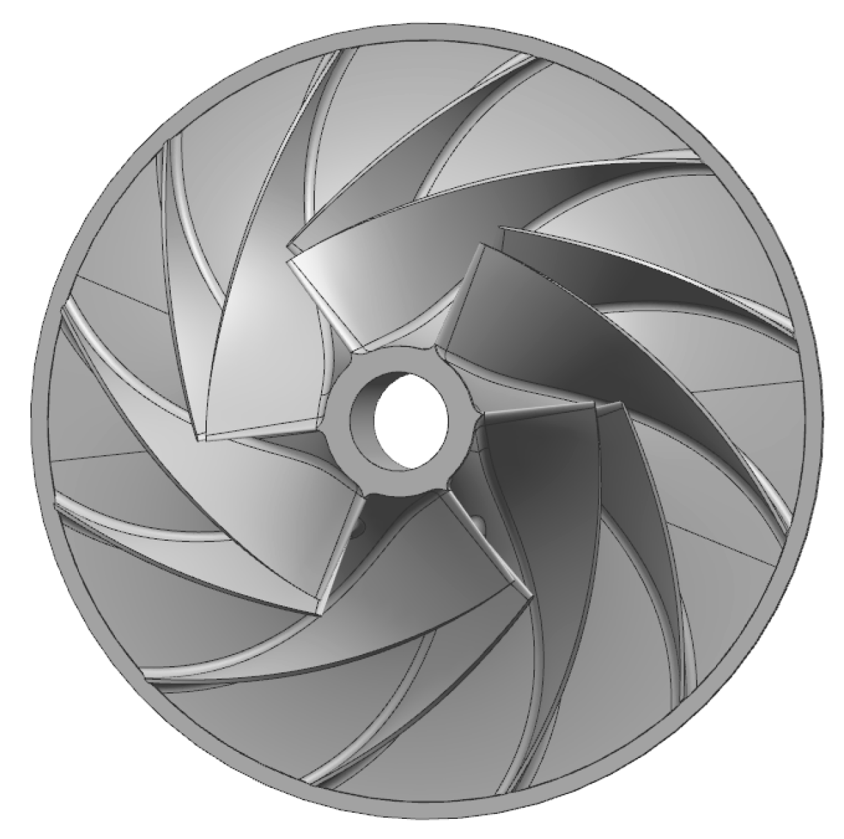
Then, a three-dimensional (3D) model is obtained. Subsequently, 3D computational fluid dynamics (CFD) simulation software is used to analyze and optimize the performance parameters. During the 3D simulation process, the governing equations are established in a rotating Cartesian coordinate system. The turbulence calculation equation adopts the Reynolds-Averaged Navier–Stokes (RANS) method, and the turbulence model used is the Shear Stress Transport (SST) k-ω model. After further analyses and optimization of the impeller’s sweep angle and back sweep angle, the final compressor impeller model is obtained as shown in Figure 2. The compressor impeller consists of a total of 6 main blades and splitter blades.

Based on the 3D model, a corresponding experimental platform for the compressor was constructed, where the outlet and inlet pressures of the compressor were measured using multiple pressure probes. The measurement error for the inlet pressure was below 0.03 kPa, while the measurement error for the outlet pressure was below 0.3 kPa. Temperature measurements at the inlet and outlet were carried out using thermocouples, with a temperature error below 0.15 K. By using the corresponding formulas, the pressure ratio and isentropic efficiency were calculated, and the results were compared with the calculations from the 3D model for validation. When the validation of the model is confirmed, the 3D calculations can be appropriately and uniformly expanded to generate additional data points for the compressor, facilitating subsequent prediction using data-driven methods.

Figure 3 shows the partial characteristic curve of the centrifugal compressor. The flow rate varies only within a certain range at a fixed speed, and the compression ratio becomes more sensitive to changes in flow rate as the speed increases, with the opposite isentropic efficiency. The compressor at a certain speed flow decreases to a certain value; the compression ratio increases to the limit value. Then, the gas flow will produce strong pulsation or even backflow and blade vibration. Thus, the minimum flow rate at each speed to connect the boundary line is called the surge boundary. Similarly, when the flow rate increases to a certain value, the compression ratio and isentropic efficiency begin to fall sharply, and the flow rate cannot be increased any further. The boundary line connecting the maximum flow rate values at each speed is called the choking boundary.

To facilitate the use of existing data to find the compression ratio and isentropic efficiency corresponding to a certain flow rate at each speed, the assist variable $\beta$ is introduced, i.e., in the flow rate range of each speed, n operating points are taken according to the flow bandwidth range according to the serial number, and the operating points of the same serial number obtained at each speed are connected in turn. The $\beta$ line schematic is shown in Figure 4. The operating points are uniformly obtained at iso speed lines. If there are changes in the operating points on the compressor characteristic curve, $\beta$ assist lines need to be made in order.

Once the reduced speed and $\beta$ values have been determined, three two-dimensional (2D) interpolation tables can be formed from the available characteristic data. Reduced flow rate, compression ratio, and isentropic efficiency can all be calculated through $\beta$ and reduced speed. The above relationship transformation is shown in Figure 5.

The speed range for the compressor characteristic data in this paper is 10,000 r/min to 90,000 r/min, with 1 set of intervals per 10,000 r/min, for a total of 9 sets of speed data. Thus, 25 points are taken in the flow range for each speed, so $\beta$ is taken as all integers between 1 and 25. To obtain the SVM training data, Latin hypercube sampling (LHS) was used to randomly select 1000 initial training sample data points in the 2D space of the corresponding range of values of the speed and $\beta$, and the interp2 function in MATLAB was used to interpolate the sample data. After the calculation was performed, 1000 sets of speed flow/compression ratio/isentropic efficiency data can be obtained as an initial training sample, in which interp2 can be chosen from either the linear interpolation algorithm (input linear) or the cubic spline interpolation algorithm (input cubic). For each of the 2 algorithms, 1000 sets of data are taken in this paper. The accuracy of both is compared in the subsequent section. Meanwhile, subsequent sections will conduct data sensitivity analysis of the model, and the training samples used will also be selected from these 1000 sets of data.

2.2. GA-SVM

Compared with traditional neural networks, the topology of the SVM is determined by support vectors, which can avoid the problem of conventional neural networks that need to be repeatedly adapted to determine the network structure. In contrast, the SVM uses nonlinear kernel functions to map the original vectors to a high-dimensional feature space, ensuring the good generalization of the model and overcoming the issue of dimensionality [21]. The SVM can be used for pattern classification and regression, and in this paper, it is applied to regression. Then, 2 regression-type SVMs were built, both with inputs of the speed and flow and outputs of the compression ratio and isentropic efficiency.

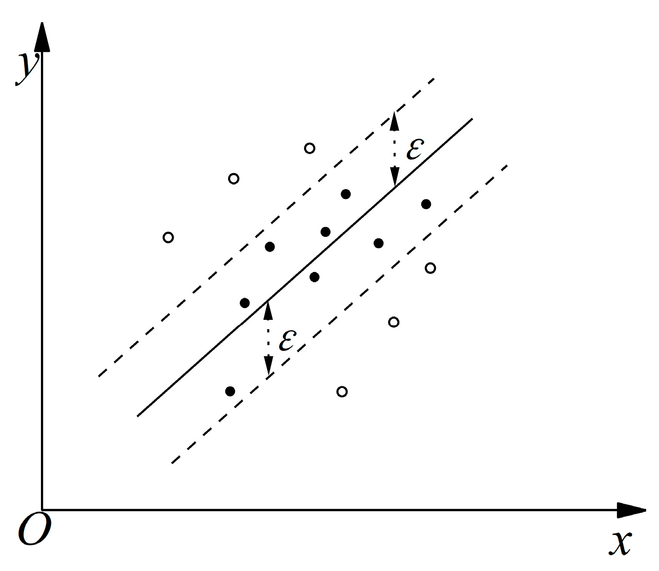
The detailed derivation theory of the SVM can be found in the work content of Cristianini, N [22]. This paper provides only a brief overview. When used for regression, the SVM usually builds the model; the main idea of the SVM is to create a surface so that the error of all sample points from the surface is minimized. In general regression, the error loss is only 0 if the output value of the regression model is equal to the original sample value. Nevertheless, in a regression-type SVM, an allowable error value $\epsilon$ is usually set, and the error loss is considered to be 0 if the sample points are within $\epsilon$ distance from the surface. As shown in Figure 6, points within the error band are represented by solid points, while others are represented by hollow points. Solid points can default to an error of 0. $\epsilon$ is called the insensitive loss function parameter, and the larger the value of this parameter is, the smaller the number of support vectors and the lower the regression accuracy.

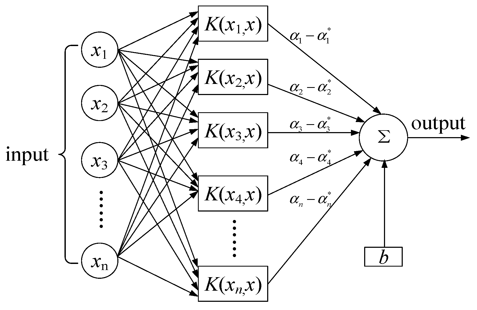
Figure 7 shows the basic structure of the SVM. For ease of understanding, it can be assumed that there is a training sample $\{(x_i,y_i),i=1,2\dots n\}.$, where $n$ is the sample size, $x_i$ is the input column vector, $x_i\in R^d$, $y_i$ is the corresponding output value, and $y_i\in R$. The linear regression function in the high-dimensional feature space is shown in Formula (1), and the insensitive loss function described above is defined in Formula (2).

$$y=w\cdot \phi (x)+b$$

(1)

$$L(\epsilon )=\{\begin{array}{l}0,\left|y-f(x)\right|<\epsilon \\ \left|y-f(x)\right|-\epsilon ,\left|y-f(x)\right|\ge \epsilon \end{array}$$

(2)

$\phi (x)$ in Formula (8) is the nonlinear mapping function, while $w$ and $b$ are the weight vector and deviation, respectively. According to the computational theory of the SVM [23], the problem of finding the optimal surface can be transformed into the optimization problem in Formula (3).

$$\{\begin{array}{l}\min \frac{1}{2}{\Vert w\Vert }^2+C{\displaystyle \sum _{i=1}^n({\xi }_i+{\xi }_i^{*})}\\ s.t.\{\begin{array}{l}{y}_i-w\cdot \phi (x_i)-b\le \epsilon +{\xi }_i\\ -y_i+w\cdot \phi (x_i)+b\le \epsilon +{\xi }_i^{*}\\ {\xi }_i\ge 0,{\xi }_i^{*}\ge 0\end{array}, i=1,2,\dots ,n\end{array}$$

(3)

$\xi$ and ${\xi }^{*}$ are slack variables that prevent overfitting of the SVM. $C$ is the penalty factor. Moreover, a more significant value of $C$ indicates a larger penalty for data points beyond the $\epsilon$ band when the SVM fits better, but too large $C$ will lead to poor model generalization. After using the Lagrangian function for the optimal solution [24], the final regression function is obtained, as shown in Formula (4).

$$f(x)={\displaystyle \sum _{i=1}^n({\alpha }_i-{\alpha }_i^{*})K(x_i,x)+b}$$

(4)

where ${\alpha }_i$ and ${\alpha }_i^{*}$ are the Lagrangian multipliers, and the solution corresponding to the nonzero multiplier is the support vector. $K(x_i,x)$ is the kernel function, and the Gaussian kernel function is chosen for the SVM in this paper, whose expression is Formula (5).

$$K(x_i,x)=\exp (-\frac{\left|\right|x_i-x|{|}^2}{2{\sigma }^2})$$

(5)

where $\gamma =\frac{1}{2{\sigma }^2}$ and $\gamma$ are the kernel coefficient; the larger its value, the narrower the Gaussian distribution. The model only acts near the support vector, which is accessible to overfit; if the value of $\gamma$ is too large, the Gaussian distribution is too smooth, and the fit is not good.

In nonlinear regression-type SVM, common kernel functions include the Gaussian kernel function, the sigmoid kernel function, and the polynomial kernel function [25]. In this paper, the Gaussian kernel function was adopted due to the fact that the Gaussian function can adapt to various complex nonlinear relationships. Although the sigmoid kernel function can also adapt to some nonlinear relationships, its adaptability is weaker compared to that of the Gaussian kernel function. As the degree of the polynomial kernel function increases, it is prone to overfitting. In contrast, the Gaussian kernel function is mapped through the Gaussian distribution function, which can map data to an infinite dimensional space and has a stronger fitting ability [26,27]. Therefore, this paper will demonstrate the accuracy of the Gaussian kernel functions in Section 3. The definitions of the polynomial kernel functions and sigmoid kernel functions are as follows:

$$K(x_i,x)={(\gamma x_i{}^{T}x+r)}^d$$

(6)

$$K(x_i,x)=\tanh (\gamma x_i{}^{T}x+r)$$

(7)

$\gamma$ also represents the kernel coefficient. $r$ is the constant coefficient.

In summary, it can be found that the performance of the SVM for regression prediction depends mainly on the insensitive loss function parameter $\epsilon$, the penalty factor $C$, and the kernel coefficient $\gamma$. The insensitive loss function parameter $\epsilon$ can be set according to the numerical accuracy of the sample data. At the same time, it is challenging to determine the values of the penalty factor $C$ and the kernel coefficient $\gamma$; thus, the use of optimization methods to find the best combination of these 2 parameters will be the key to determining whether the SVM can accurately predict the performance of the compressor [28].

The GA is an intelligent optimization algorithm combining biological genetic and evolutionary mechanisms, which has the advantages of a good applicability and a high probability of finding the best and fastest search speed. The computational process of the GA mainly includes the encoding, initial population, calculation of fitness value, and three basic operations of selection, crossover, and variation. In this paper, the GA is used to optimize the penalty factor $C$ and kernel coefficient $\gamma$ of the SVM. The specific flow chart is shown in Figure 8.

Using 1000 sets of data points previously obtained by $\beta$-line-assisted interpolation as the training sample and 225 sets of known data points of the compressor characteristics as the test sample, the GA optimization process was carried out to determine the range of values for the penalty factor $C$ and the kernel coefficient $\gamma$. The range of values for $C$ was selected to be (0, 100), and the range of values for $\gamma$ was chosen to be [0, 1000]. Then, the initial population was coded and generated with a population size of 40. The SVM model is invoked to calculate the mean squared error (MSE) of the training sample as the fitness value of the individuals. The termination condition of the GA is that the number of iterations of population genetics reaches 50. If the termination condition is not reached, a loop iteration is performed. When the termination condition is reached, the penalty factor $C$ and the kernel coefficient $\gamma$ with the lowest MSE are removed to decode and train the SVM with this combination of parameters. The generalizability of the model is verified using a test sample at the end of the training.

2.3. Evaluation Indicators

The performance indicators of the model generalization are the root mean squared error (RMSE), mean absolute error (MAE), and MAPE. The definition of the above performance indicators is as follows: [29,30].

$$RMSE=\sqrt{\frac{1}{n}\sum _{i=1}^n{\left({\widehat{y}}_i-y_i\right)}^2}$$

(8)

$$MAE=\frac{1}{n}\sum _{i=1}^n\left(\left|{\widehat{y}}_i-y_i\right|\right)$$

(9)

$$MAPE=\frac{1}{n}\sum _{i=1}^n\left(\left|\frac{{\widehat{y}}_i-y_i}{y_i}\right|\right)\times 100\%$$

(10)

${\widehat{y}}_i$ is the predicted value, and $y_i$ is the true value.

3. Results

In this paper, the training and testing of the compressor prediction model were conducted on a computer equipped with an AMD Ryzen 7 5800 8-Core Processor, operating at 3.40 GHz, with 16 GB of RAM and an NVIDIA GeForce GTX 1650 SUPER graphics card.

3.1. Kernel Function Selection

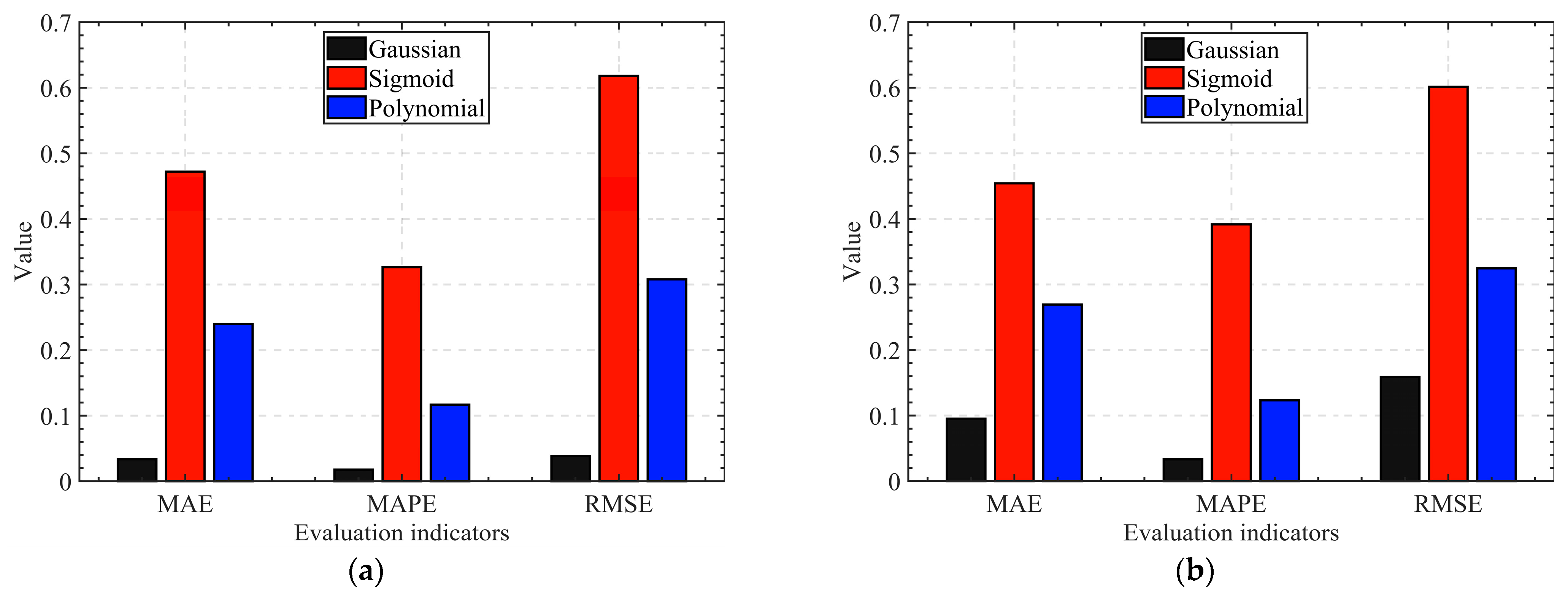
To establish an accurate prediction model in the future, it is necessary to make a preliminary selection of the kernel function of the SVM. The steps are as follows: Randomly select 200 sets of data from 225 sets of known data as a training sample, and the remaining 25 sets of data are a test sample. Train SVM using three different kernel functions. Figure 9 shows the comparison of the SVM’s performance in predicting compression ratio when using different kernel functions.

It can be found that the SVM using the Gaussian kernel function outperforms using the polynomial kernel function and sigmoid kernel function in terms of prediction performance in both training and test results. Using the Gaussian kernel functions in nonlinear regression-type SVM will result in high accuracy of the model. Therefore, all subsequent SVMs will use the Gaussian kernel functions.

3.2. Interpolation Method

The distribution of the 1000 combinations of $\beta$ and speed obtained after sampling are shown in Figure 10. Interpolating the data points in the figure allows for the calculation of 1000 combinations of flow speed/compression ratio/isentropic efficiency as a training sample.

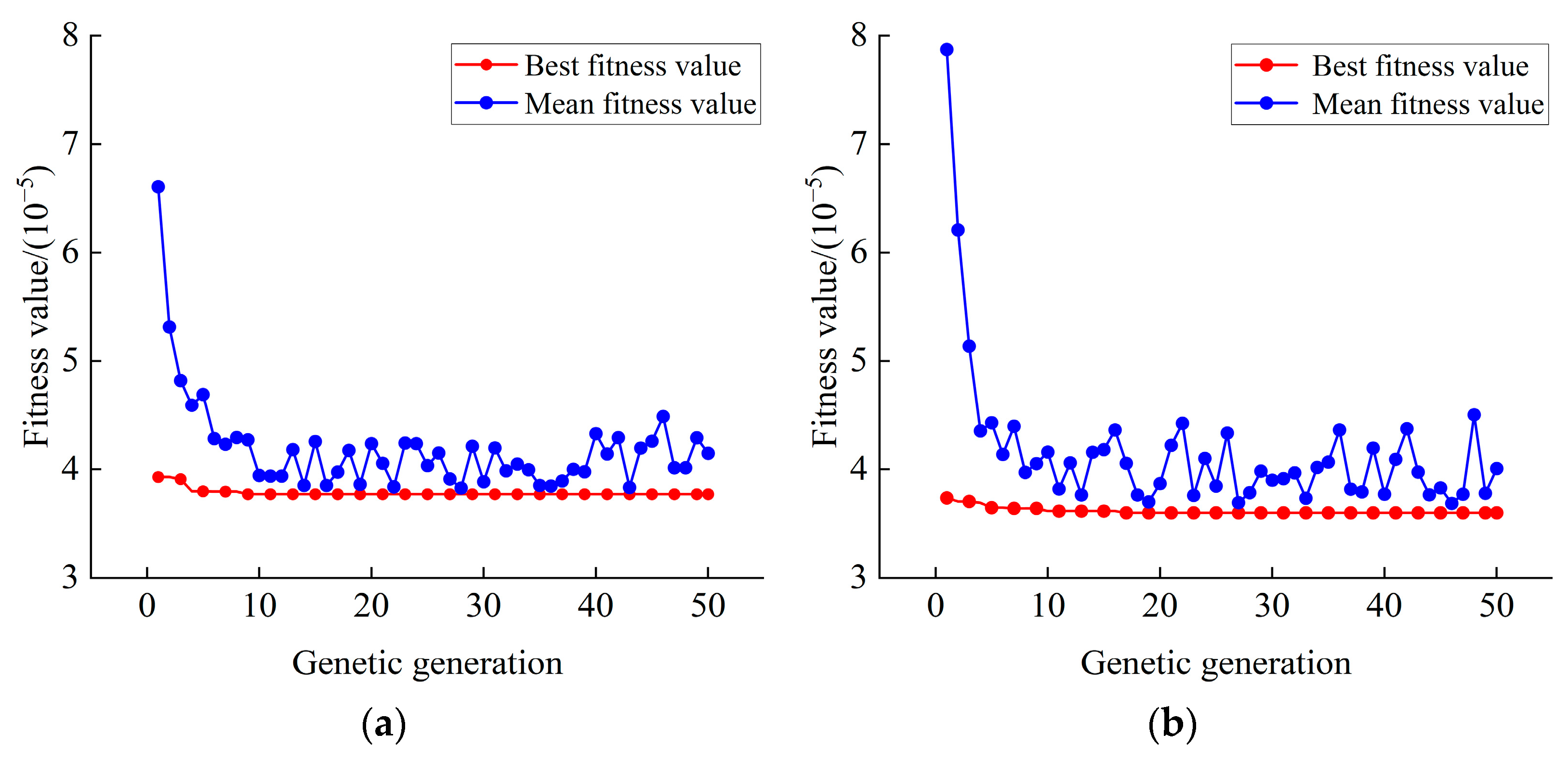
The interpolated compression ratio training samples using the linear and cubic commands were substituted into the GA-SVM program, and the changes in the resulting fitness values of both are shown in Figure 11. The best fitness value curve of both gradually decreases and stabilizes, which indicates that the genetic algorithm has a good effect on the two parameters in terms of finding the optimum.

The compression ratio and isentropic efficiency sample data obtained from the two interpolation methods were substituted into the training, and the generalization performance of the SVM was verified using a test sample (225 sets of known data points). The results of the resulting parameter selection and the model performance metrics are shown in

Table 1. Comparison of the performance of the corresponding models for the 2 interpolation methods.

Parameters	Compression Ratio (Linear)	Compression Ratio (Cubic)	Isentropic Efficiency (Linear)	Isentropic Efficiency (Cubic)
$C$	99.9012	87.5251	99.7891	99.2186
$\gamma$	36.7785	34.3228	257.0136	284.2515
RMSE	0.0475	0.0466	0.0121	0.0124
MAE	0.0395	0.0398	0.0076	0.0081
MAPE	0.0191	0.0203	0.0138	0.0145

.

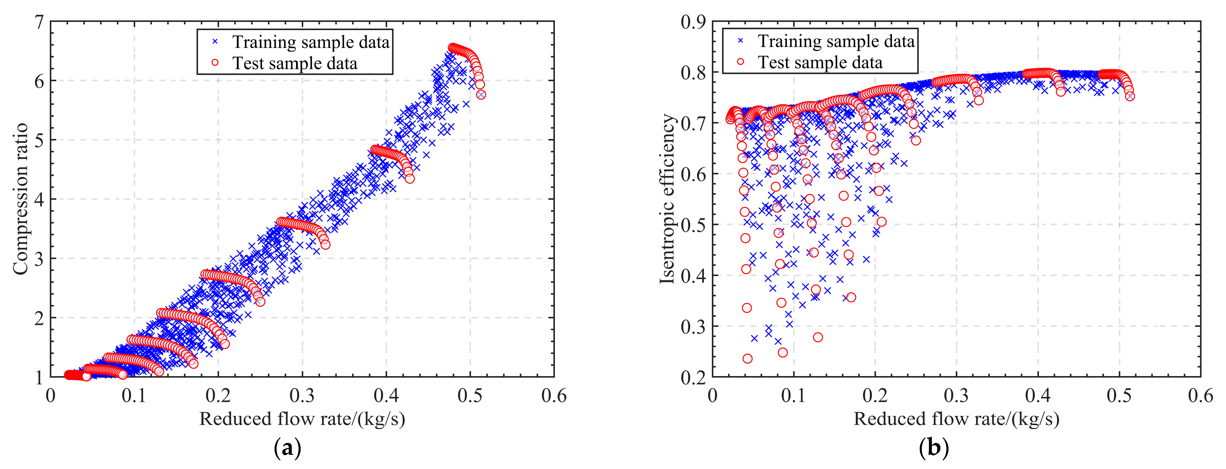
The generalization performance of the SVM trained using linear interpolation is superior in all aspects, and only the RMSE of the compression ratio is slightly higher than that of cubic spline interpolation. Thus, the compressor data obtained using linear interpolation are more accurate. Figure 12 shows the distribution of training sample data points obtained using linear interpolation.

3.3. Preliminary Comparison of Prediction Models

In this section, we will focus on comparing the prediction accuracy of the GA-SVM, the GA-BPNN, the GA-ELMNN, and the GA-GRNN, followed by conducting data sensitivity analysis on these four models.

The above three types of neural networks are widely used for nonlinear regression, and their predictive performance in terms of compressors will be compared with the GA-SVM here. GA is used to optimize the weight thresholds of the BPNN and ELMNN. Due to the number of input parameters being two, the number of neurons in the hidden layer is selected as five based on empirical values, and the genetic generations of the GA are also determined as 50. Because more parameters need to be optimized compared to the SVM, the population size is chosen as 80. There are no weights or thresholds in the GRNN, and the performance is only determined via the smoothness factor. The GA is used to optimize the smoothness factor, and the genetic generations are also 50. Since only one parameter is optimized, the population size is chosen as 30.

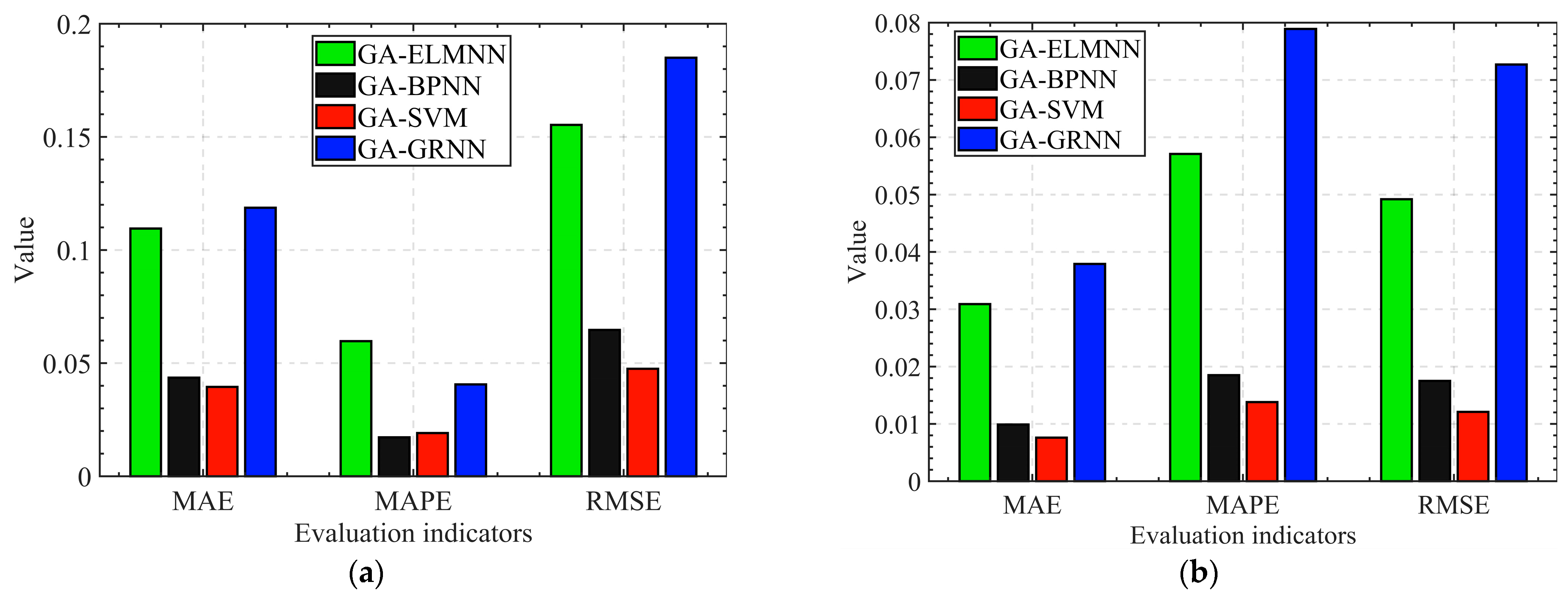
After training four models using the initial training sample in Section 3.2, the predictive performance indicators of the test sample were statistically analyzed for the models. Figure 13 shows the compressor performance prediction indicators for these four models.

It is easy to find that the prediction performance of the GA-ELMNN and GA-GRNN on compression ratio and isentropic efficiency is significantly worse than that of the GA-BPNN and GA-SVM. The prediction performance of the GA-BPNN and GA-SVM is comparable. Among them, the GA-SVM has lower performance indicators than the GA-BPNN, except for a slightly higher MAPE for predicting compression ratio than the GA-BPNN.

Table 2. Model training and test time.

Predictive Variable	Model	GA-ELMNN	GA-BPNN	GA-SVM	GA-GRNN
Compression ratio	training time (s)	216.3	1626.3	218.5	677.5
	test time (s)	0.74	1.38	0.71	0.87
Isentropic efficiency	training time (s)	1479.5	3127.9	1421.4	1536.7
	test time (s)	0.78	2.21	1.01	0.89

presents the time taken for training four models using 1000 sets of initial data points and predicting 225 sets of known data points. Among them, the GA-SVM and GA-ELMNN exhibit faster training speeds, followed by the GA-GRNN, while the GA-BPNN is the slowest. This is because the BPNN requires the use of a back-propagation algorithm to compute and update the weights and thresholds, which involves multiple iterations and gradient descent to minimize the loss function. Additionally, from Figure 12, it can be observed that the training data points for isentropic efficiency exhibit a large amount of clustering and local dispersion. On the other hand, the points for the compression ratio are relatively evenly distributed. Therefore, the training time for the isentropic efficiency prediction model is longer compared to the training time for the compression ratio prediction model. The test time for the four models, except for the GA-BPNN, is almost within 1 s. Considering that most of the prediction models are trained offline in advance before their usage, the training and test times presented in this paper serve as references. The subsequent analysis focuses more on the accuracy of the models.

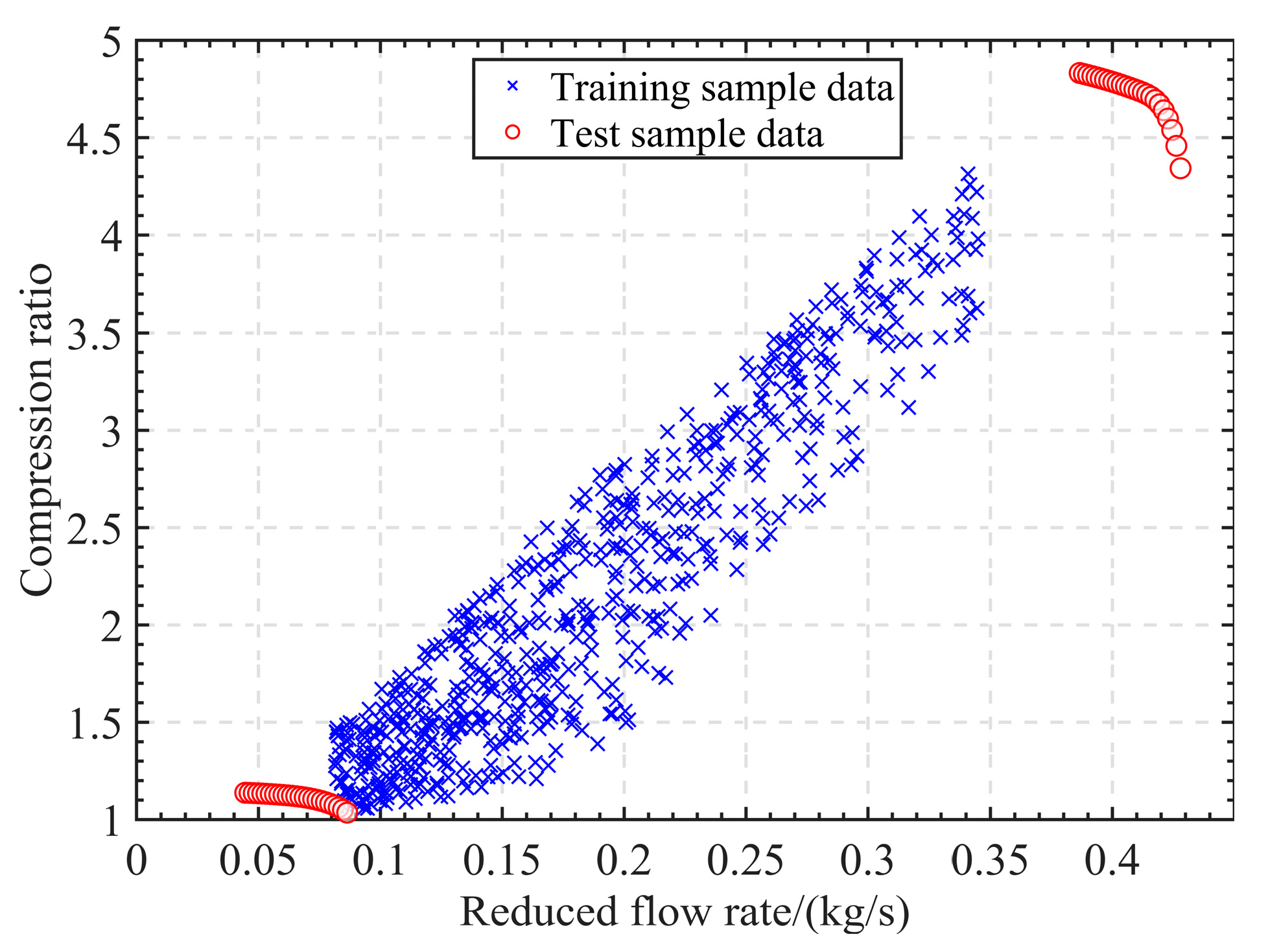
The extrapolation performance of the model is also a key factor in measuring the accuracy of the model. This paper will use compression ratio to evaluate the performance of extrapolation. The specific method is as follows: 1000 sets of initial data points are arranged in ascending order for the reduced flow rate value, and the data points with numbers of 200 to 800 are selected as extrapolation training samples. Take two sets of points at iso speed lines near the distribution region of the training samples as the test samples, as shown in Figure 14.

The test data points with a smaller reduced flow rate in the figure are the low-speed extrapolation test data points, while the larger ones are the high-speed extrapolation test points. The extrapolation results obtained from the four models are shown in Figure 15.

In the low-speed extrapolation results, except for the GA-GRNN, the trend of the extrapolated data points of the other three models is consistent with the test data points. In the high-speed extrapolation results, the trend of the four model extrapolation data points is consistent with the test data points. It is obvious to see that whether it is high-speed extrapolation or low-speed extrapolation, the extrapolation data points of the GA-SVM and GA-BPNN are closer to the test data points.

Table 3. Comparison of extrapolation performance of four models.

Model	GA-ELMNN	GA-BPNN	GA-SVM	GA-GRNN
RMSE	0.1754	0.0844	0.0609	0.1627
MAE	0.1453	0.0655	0.0372	0.1406
MAPE	0.05	0.0273	0.0159	0.0651

shows the extrapolation performance of four models.

It can be observed that in terms of extrapolation performance, the GA-SVM performs the best. The RMSE of the GA-SVM is only 0.0609, 167% lower than the GA-GRNN and 188% lower than the GA-ELMNN. The extrapolation performance of the GA-BPNN is slightly worse than the GA-SVM.

To comprehensively evaluate the performance of these models, this section will also conduct a data sensitivity analysis. The effects of training sample size on prediction accuracy will be investigated. Set the sample size to 800, 600, 400, and 200. Randomly sample 1000 sets of initial training data points based on sample size values to obtain new training samples. The test sample is still selected as the known 225 data points.

From Figure 12b, it can be observed that the compression ratio training sample data point distribution is more uniform compared to isentropic efficiency, and the randomly obtained small size sample will also be more uniform. Therefore, the effects of different sample sizes on the overall prediction accuracy of the model compression ratio will be evaluated here. Figure 16 shows the RMSE of the compression ratio prediction results for four models as a function of sample size.

It can be observed that the prediction accuracy of the GA-ELMNN continues to improve with the increase in sample size, while the GA-GRNN remains almost unchanged. However, the overall prediction accuracy of the GA-ELMNN and GA-GRNN is still lower than that of the GA-SVM and GA-BPNN. The prediction accuracy of the GA-BPNN and GA-SVM remains consistent with the trend of sample size changes. As the sample size is below 600, the prediction accuracy of the GA-BPNN and GA-SVM will begin to decrease. As the sample size is between 600 and 1000, the numerical variation in RMSE is not significant. This indicates that the GA-SVM and GA-BPNN have better generalization, and reducing the number of training samples to a certain extent can still maintain good prediction accuracy.

Both the GA-SVM and the GA-BPNN have good predictive performance. The next section will give the error of each prediction point and focus on studying the detailed differences between the two models.

3.4. Further Comparison of the GA-SVM and GA-BPNN

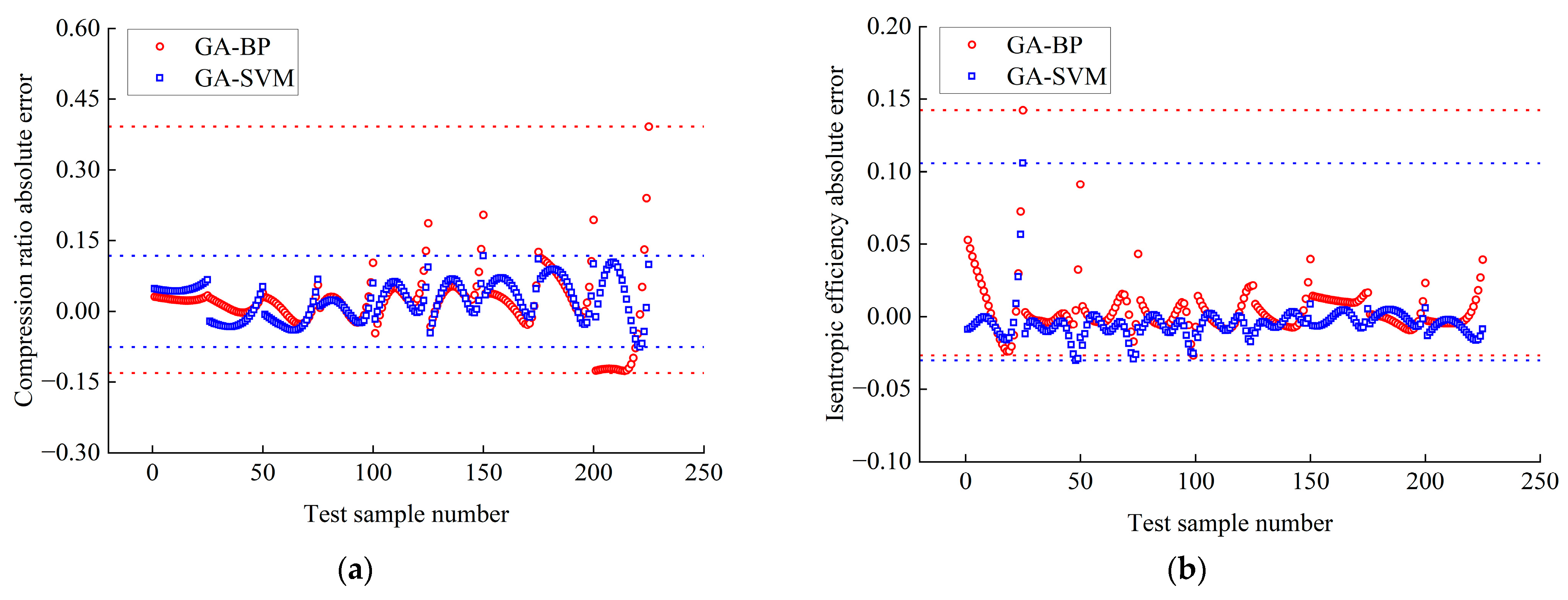
Since both methods have high prediction accuracy, to facilitate the observation of the difference between the two models, the error of fitting the GA-BPNN and GA-SVM test sample is calculated in this paper, and the distribution is shown in Figure 17. In Figure 13a, the MAPE of the GA-BPNN predicted compression ratio is slightly lower than the GA-SVM. From Figure 17a, it can be observed that the reason for this phenomenon is that when the test sample number is between 1 and 70, the error value predicted by the GA-BPNN fluctuates less. These data lead to a certain decrease in the MAPE of the GA-BPNN prediction compression ratio.

However, in terms of the prediction of the compression ratio and isentropic efficiency, the error band of the GA-SVM is smaller than that of the GA-BPNN. At the same time, it can be intuitively seen from the figure that the overall degree of fluctuation in the error data of the compression ratio and isentropic efficiency predicted by the GA-SVM is minor. Considering the overall predictive performance of the model, the GA-SVM predicts better performance metrics than the GA-BPNN.

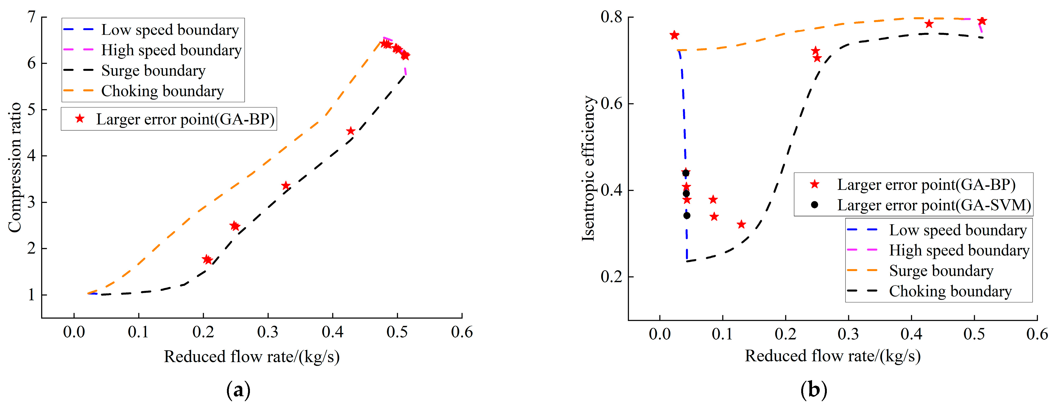
Figure 18 shows the locations of the GA-BPNN and GA-SVM larger error points in the compressor flow and speed operating regions when using 1000 sets of training data. The numbers of the more significant error points in the test sample were queried and located according to Figure 17 (the GA-SVM is more accurate in predicting the compression ratio; thus, there are no more significant points in Figure 18a with regards to the GA-SVM error). It was found that the GA-BPNN predicted the compression ratio close to the choking boundary, and the high-speed boundary was poorer. The compression ratio prediction is poor. The larger error points of the GA-BPNN for isentropic efficiency prediction are mainly concentrated in high-speed and low-speed boundaries. The larger error points of the GA-SVM prediction are primarily focused near the choking boundary, mainly because the isentropic efficiency is too sensitive to the flow rate change at a fixed speed in the low-speed boundary. The phenomenon that the GA-BPNN has a significant bias in predicting data in the boundary is known as the marginal effect [14], as only sample data from one of the sides of the boundary are available during training, resulting in a loss of fitting accuracy. Nevertheless, this phenomenon does not occur with the GA-SVM; therefore, the GA-SVM is considered to have a better generalization.

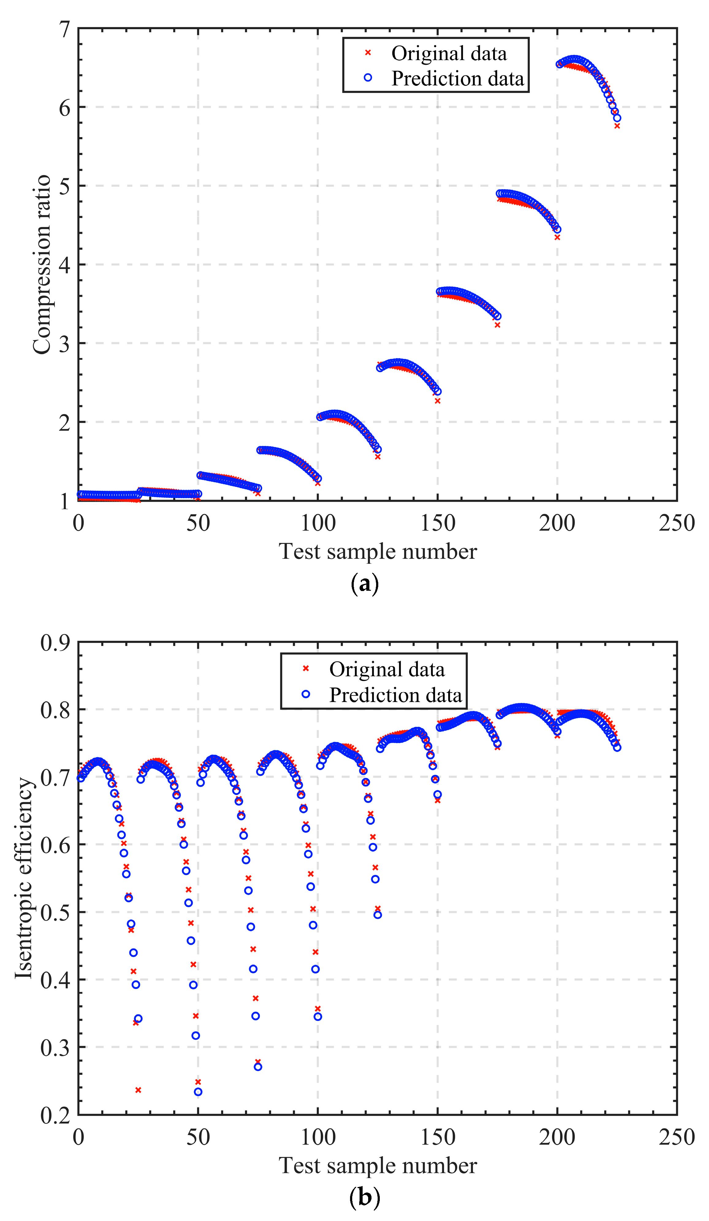
Figure 19 shows the final GA-SVM predicted data compared to the original data. The compression ratio prediction is very accurate, although there is a small deviation in the prediction of the isentropic efficiency at the boundary. However, considering that the actual operation of the compressor will be far from each boundary, it can be considered that the model can be applied in engineering and simulation.

3.5. Optimization of Original Data

In this paper, we have a total of 225 known data points. Obtaining the characteristic points of the compressor, whether through simulation or experimentation, is both expensive and tedious. Therefore, in this section, we will employ the GA-SVM to optimize the known data points to ensure that a predictive model can be established with a smaller amount of known data.

From Section 3.3, we can infer that a training sample size of 600 allows the GA-SVM to maintain good predictive performance. Therefore, we fix the number of interpolated points at 600. On nine iso speed lines, data points were uniformly sampled at multiples of five, resulting in five sets of original data points with quantities of 45, 90, 135, 180, and 225, respectively.

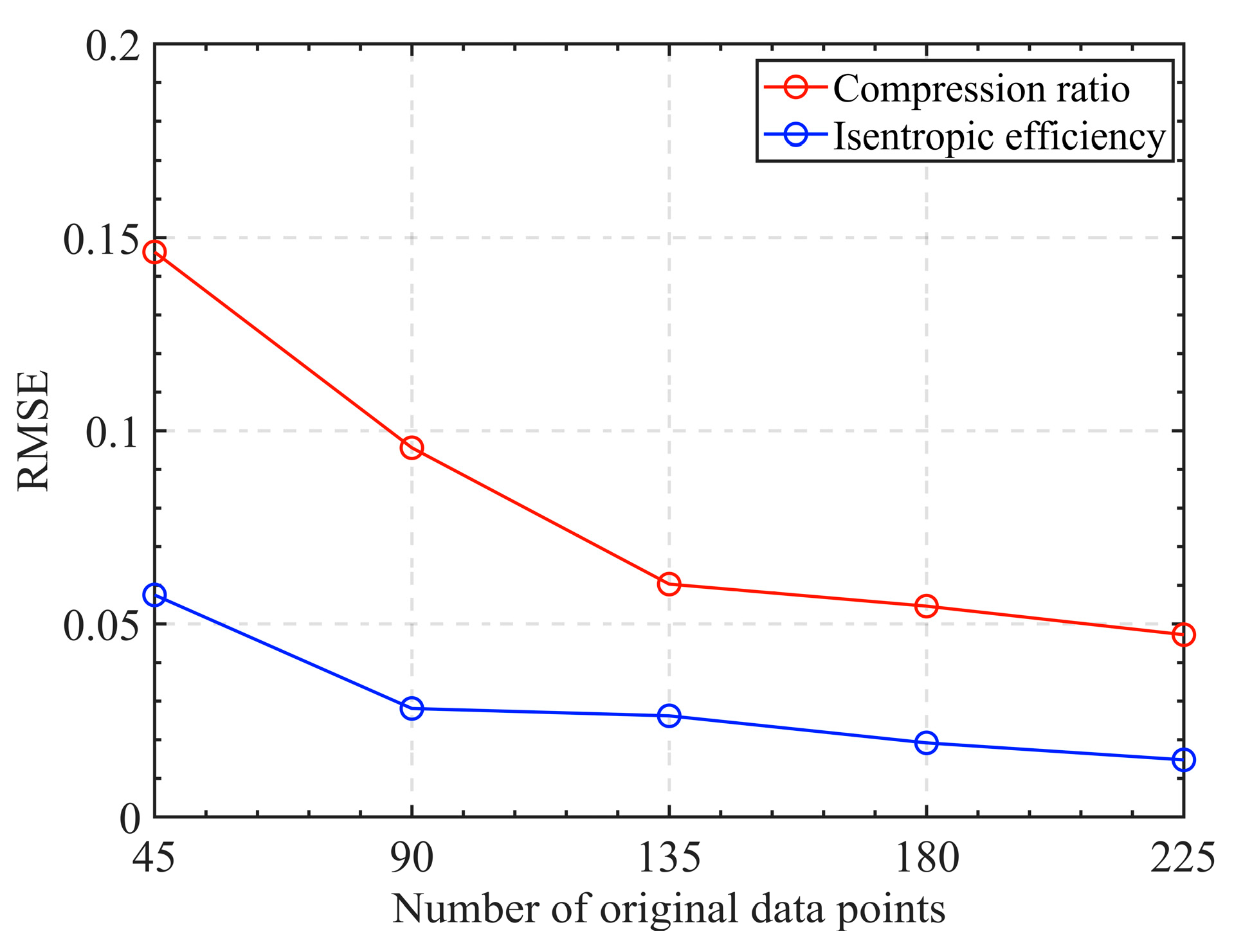
The GA-SVM is trained using training samples obtained by interpolating different sets of original data points. We still use the known 225 data points for testing. Figure 20 shows the variation in RMSE of the prediction results with the number of original data points.

When the number of original data points is below 135, the predictive performance of the GA-SVM for the compression ratio starts to vary dramatically. In contrast, the predictive performance of the GA-SVM for isentropic efficiency starts to vary dramatically when the number of original data points falls below 90. The reason for this difference is that the points on the compression ratio curve are widely distributed, and reducing the number of original points significantly alters the characteristics of the curve itself. On the other hand, the points on the isentropic efficiency curve are relatively close together at medium to high speeds, so reducing the number of original points does not have a significant impact on it.

In summary, using 135 original data points still enables the GA-SVM to maintain high predictive accuracy. This reduces the workload of acquiring 40% of the original data points. However, if there is a higher tolerance for prediction errors, further reducing the number of original data points is also feasible.

4. Conclusions

Based on the characteristic curves of a compressor model, a training sample of compressor characteristic data was obtained using the $\beta$-line-assisted interpolation method. The corresponding model was built in MATLAB to predict the compression ratio and isentropic efficiency of the compressor. The main conclusions are as follows.

(1)

As SVM is used for compressor performance prediction, Gaussian kernel functions can achieve high prediction accuracy. Preliminary training and testing of 200 sets of training sample data and 25 sets of test sample data were carried out. The MAE, MAPE, and RMSE of the predicted results for the training sample are 0.0337, 0.0177, and 0.0385, respectively. The MAE, MAPE, and RMSE of the predicted results for the test sample are 0.0952, 0.0334, and 0.1589, respectively. These two sets of evaluation indicators are superior to the sigmoid kernel function and the polynomial kernel function.

(2)

The training samples obtained using the linear interpolation method were found to be more accurate, corresponding to a higher prediction accuracy of the GA-SVM. At this point, the GA-SVM kernel coefficient $\gamma$ for predicting compression ratio is 36.7785, and the penalty factor $C$ is 99.9012; the GA-SVM kernel coefficient for predicting isentropic efficiency $\gamma$ is 257.0136, and the penalty factor $C$ is 99.7891.

(3)

Train four models using 1000 initial training samples from Section 3.2. The GA-SVM and GA-BPNN have significantly better prediction accuracy in compression ratio and isentropic efficiency than the GA-ELMNN and GA-GRNN. The MAPE of GA-SVM predicted compression ratio results is slightly higher than GA-BPNN, and all other performance indicators are better than GA-BPNN. In addition, the GA-SVM and GA-BPNN also outperform the GA-ELMNN and GA-GRNN in terms of extrapolation performance. In data sensitivity analysis, GA-SVM and GA-BPNN can maintain almost unchanged accuracy when the training sample sizes are 600, 800, and 1000.

(4)

Analyzing the error size of 225 test data points from GA-SVM and GA-BPNN, it was found that the error band of the GA-BPNN was larger than that of the GA-SVM in terms of the compression ratio and isentropic efficiency prediction results. The GA-SVM needs to be more accurate in predicting boundary data points. After comprehensive comparison and detailed analysis, the generalization of the GA-SVM is better than the GA-BPNN. Furthermore, reducing the number of original data points to 135 still allows the GA-SVM to maintain a high level of predictive accuracy.

References

1. Liu, Y.; Chen, J.; Cheng, J.; Xiang, H. Aerodynamic Optimization of Transonic Rotor Using Radial Basis Function Based Deformation and Data-Driven Differential Evolution Optimizer. Aerospace 2022, 9, 508. [Google Scholar] [CrossRef]
2. Xin, R.; Zhai, J.; Liao, C.; Wang, Z.; Zhang, J.; Bazari, Z.; Ji, Y. Simulation Study on the Performance and Emission Parameters of a Marine Diesel Engine. J. Mar. Sci. Eng. 2022, 10, 985. [Google Scholar] [CrossRef]
3. Kovač Kralj, A. Improving Electricity Generation The Product Reaction Loop and the Use of Exhaust Gas for Co-Product Production Using Polyethylene Waste and Flue Gas or Wood. Processes 2022, 10, 2251. [Google Scholar] [CrossRef]
4. Kurzke, J.; Riegler, C. A New Compressor Map Scaling Procedure for Preliminary Conceptional Design of Gas Turbines. In Turbo Expo: Power for Land, Sea, & Air; ASME: New York, NY, USA, 2000. [Google Scholar]
5. Huang, S.; Yang, C.; Chen, H.; Zhou, N.; Tucker, D. Coupling impacts of SOFC operating temperature and fuel utilization on system net efficiency in natural gas hybrid SOFC/GT system - ScienceDirect. Case Stud. Therm. Eng. 2022, 31, 101868. [Google Scholar] [CrossRef]
6. Zhong, M.P. Analysis and optimum design for the transient thermal process of a two-stage compressor under alternating working conditions. Appl. Therm. Eng. 2016, 103, 28–37. [Google Scholar] [CrossRef]
7. Zhou, K.; Liu, S.M. Prediction of a Compressor’s Performance Based on Data and Neural Networks. Therm. Turbine 2017, 46, 158–163. [Google Scholar]
8. Huang, W.; Chang, J.; Sun, Z.B. Characteristic Curve Prediction of Compressor Based on MEA-BP Neural Network. J. Chongqing Univ. Technol. (Nat. Sci.) 2019, 33, 67–74. [Google Scholar]
9. Xie, X.Y.; Lu, Y.M.; Wang, X.F.; Wang, W. Simulation investigation on dynamic performance of single shaft gas turbine based on different compressor characteristic curve prediction methods. J. Eng. Therm. Energy Power 2021, 36, 26–34. [Google Scholar]
10. Fang, Y.L.; Liu, D.F.; He, X.; Yu, L.W.; Deng, Z.M. Research on the precise step fitting method of compressor characteristic map. Gas Turbine Exp. Res. 2019, 32, 21–27. [Google Scholar]
11. Tsoutsanis, E.; Meskin, N.; Benammar, M.; Khorasani, K. A component map tuning method for performance prediction and diagnostics of gas turbine compressors. Appl. Energy 2014, 135, 572–585. [Google Scholar] [CrossRef] [Green Version]
12. Ghorbanian, K.; Gholamrezaei, M. An artificial neural network approach to compressor performance prediction. Appl. Energy 2009, 86, 1210–1221. [Google Scholar] [CrossRef]
13. Zheng, H.T.; Pan, F.M.; Yang, R. Performance calculation of compressor based on object-oriented method. J. Aerosp. Power 2014, 29, 140–145. [Google Scholar]
14. Lu, X.K.; Zhang, S.J.; Chi, J.L.; Wang, B. Research on the Fitting Method of Compressor Performance Curve based on Genetic Algorithm. J. Eng. Therm. Energy Power 2022, 37, 105–109. [Google Scholar]
15. Fei, J.; Zhao, N.; Shi, Y.; Feng, Y.; Wang, Z. Compressor performance prediction using a novel feed-forward neural network based on Gaussian kernel function. Adv. Mech. Eng. 2016, 8, 1687814016628396. [Google Scholar] [CrossRef] [Green Version]
16. Gholamrezaei, M.; Ghorbanian, K. Compressor map generation using a feed-forward neural network and rig data. Proc. Inst. Mech. Eng. Part A J. Power Energy 2010, 224, 97–108. [Google Scholar] [CrossRef]
17. Zhou, W.; Lu, S.; Huang, J.; Pan, M.; Chen, Z. A Novel Data-Driven-Based Component Map Generation Method for Transient Aero-Engine Performance Adaptation. Aerospace 2022, 9, 442. [Google Scholar] [CrossRef]
18. Ying, Y.; Xu, S.; Li, J.; Zhang, B. Compressor performance modelling method based on support vector machine nonlinear regression algorithm. R. Soc. Open Sci. 2020, 7, 191596. [Google Scholar] [CrossRef] [Green Version]
19. Jiang, A.W.; Xie, S.S. Method to achieving compressor characteristics based on support vector machine (SVM) and particle swarm optimization (PSO). J. Aerosp. Power 2010, 25, 2571–2577. [Google Scholar]
20. Xu, S.Y.; Ying, Y.L.; Zhou, H.Y.; JIN, Y.F.; XIE, Q.Y. Expression of Compressor Characteristic Line Based on Artificial Bee Colony Optimization Support Vector Machine Parameters. Gas Turbine Technol. 2020, 33, 24–33. [Google Scholar]
21. Du, X.; Zhou, K.; Cui, Y.; Wang, J.; Zhou, S. Mapping Mineral Prospectivity Using a Hybrid Genetic Algorithm–Support Vector Machine (GA–SVM) Model. ISPRS Int. J. Geo-Inf. 2021, 10, 766. [Google Scholar] [CrossRef]
22. Cristianini, N.; Shawe-Taylor, J. An Introduction to Support Vector Machines; Cambridge University Press: Cambridge, UK, 2000. [Google Scholar]
23. Smola, A.J.; Scholkopf, B. A tutorial on support vector regression. Stat. Comput. 2004, 14, 199–222. [Google Scholar] [CrossRef] [Green Version]
24. Duan, H.; Yin, X.; Kou, H.; Wang, J.; Zeng, K.; Ma, F. Regression prediction of hydrogen enriched compressed natural gas (HCNG) engine performance based on improved particle swarm optimization back propagation neural network method (IMPSO-BPNN). Fuel 2023, 331, 125872. [Google Scholar] [CrossRef]
25. Wang, H.; Ji, C.; Shi, C.; Ge, Y.; Wang, S.; Yang, J. Development of cyclic variation prediction model of the gasoline and n-butanol rotary engines with hydrogen enrichment. Fuel 2021, 299, 120891. [Google Scholar] [CrossRef]
26. Ji, C.; Wang, H.; Shi, C.; Wang, S.; Yang, J. Multi-objective optimization of operating parameters for a gasoline Wankel rotary engine by hydrogen enrichment. Energy Convers. Manag. 2021, 229, 113732. [Google Scholar] [CrossRef]
27. Shen, W.; Guo, X.; Wu, C.; Wu, D. Forecasting stock indices using radial basis function neural networks optimized by artificial fish swarm algorithm. Knowl.-Based Syst. 2011, 24, 378–385. [Google Scholar] [CrossRef]
28. Jing, L.L.; Yu, Y.Q. GNSS-IR soil moisture inversion method based on GA-SVM. J. Beijing Univ. Aeronaut. Astronaut. 2019, 45, 486–492. [Google Scholar]
29. Wang, H.; Ji, C.; Yang, J.; Ge, Y.; Wang, S. Implementation of a novel dual-layer machine learning structure for predicting the intake characteristics of a side-ported Wankel rotary engine. Aerosp. Sci. Technol. 2023, 132, 108042. [Google Scholar] [CrossRef]
30. Wang, H.; Ji, C.; Su, T.; Shi, C.; Ge, Y.; Yang, J.; Wang, S. Comparison and implementation of machine learning models for predicting the combustion phases of hydrogen-enriched Wankel rotary engines. Fuel 2022, 310, 122371. [Google Scholar] [CrossRef]
Figure 1. Relationship between input and output parameters of the compressor.
Aerospace 10 00558 g001
Figure 2. 3D model of the cogeneration compressor impeller.
Aerospace 10 00558 g002
Figure 3. Compressor characteristic curves. (a) Compression ratio; (b) isentropic efficiency.
Aerospace 10 00558 g003
Figure 4. Schematic diagram of β -line-assisted interpolation.
Aerospace 10 00558 g004
Figure 5. Parameter relationship transformation.
Aerospace 10 00558 g005
Figure 6. Allowable error band in the SVM.
Aerospace 10 00558 g006
Figure 7. Schematic diagram of the SVM structure.
Aerospace 10 00558 g007
Figure 8. GA-SVM flow chart.
Aerospace 10 00558 g008
Figure 9. SVM prediction performance of different kernel functions. (a) Training result; (b) test result.
Aerospace 10 00558 g009
Figure 10. Distribution of data points from the training sample.
Aerospace 10 00558 g010
Figure 11. Fitness value change curve. (a) Linear; (b) cubic.
Aerospace 10 00558 g011
Figure 12. Distribution of training sample data points obtained using linear interpolation. (a) Compression ratio; (b) isentropic efficiency.
Aerospace 10 00558 g012
Figure 13. Model prediction performance. (a) Compression ratio; (b) isentropic efficiency.
Aerospace 10 00558 g013
Figure 14. Sample distribution for evaluating extrapolation performance.
Aerospace 10 00558 g014
Figure 15. Extrapolation results of four models. (a) Low speed; (b) high speed.
Aerospace 10 00558 g015
Figure 16. The RMSE of predicted results with different compression ratios of models varies with sample size.
Aerospace 10 00558 g016
Figure 17. Test sample prediction error distribution. (a) Compression ratio; (b) isentropic efficiency.
Aerospace 10 00558 g017
Figure 18. Region of the distribution of larger error points. (a) Compression ratio; (b) isentropic efficiency.
Aerospace 10 00558 g018
Figure 19. GA-SVM prediction results. (a) Compression ratio; (b) isentropic efficiency.
Aerospace 10 00558 g019
Figure 20. The RMSE of predicted results varies with the number of original data points.
Aerospace 10 00558 g020