Article

Kriging-Based Framework Applied to a Multi-Point, Multi-Objective Engine Air-Intake Duct Aerodynamic Optimization Problem

by
Przemysław S. Drężek
1,2,*,
Sławomir Kubacki
2 and
Jerzy Żółtak
1
1
Łukasiewicz Research Network, Institute of Aviation, 02-256 Warsaw, Poland
2
Institute of Aeronautics and Applied Mechanics, Faculty of Power and Aeronautical Engineering, Warsaw University of Technology, 00-665 Warsaw, Poland
*
Author to whom correspondence should be addressed.
Aerospace 2023, 10(3), 266; https://doi.org/10.3390/aerospace10030266
Submission received: 28 January 2023 / Revised: 5 March 2023 / Accepted: 6 March 2023 / Published: 9 March 2023

Abstract

:
The forecasted growth in dynamic global air fleet size in the coming decades, together with the need to introduce disruptive technologies supporting net-zero emission air transport, demands more efficient design and optimization workflows. This research focuses on developing an aerodynamic optimization framework suited for multi-objective studies of small aircraft engine air-intake ducts in multiple flight conditions. In addition to the refinement of the duct’s performance criteria, the work aims to improve the economic efficiency of the process. The optimization scheme combines the advantages of Kriging-based Efficient Global Optimization (EGO) with the Radial Basis Functions (RBF)-based mesh morphing technique and the Chebyshev-type Achievement Scalarizing Function (ASF) for handling multiple objectives and design points. The proposed framework is applied to an aerodynamic optimization study of an I-31T aircraft turboprop engine intake system. The workflow successfully reduces the air-duct pressure losses and mitigates the flow distortion at the engine compressor’s front face in three considered flight phases. The results prove the framework’s potential for solving complex multi-point air-intake duct problems and the capacity of the ASF-based formulation to guide optimization toward the designer’s preferred objective targets.

1. Introduction

From the time of the famous Wright brothers’ first flight, global air traffic has grown continuously regardless of economic or political turmoil. In only the last two decades, it has more than doubled. Two major commercial aircraft suppliers, Boeing and Airbus, forecast further air traffic growth in the coming decades at a rate of nearly 4% annually, which will create a demand for global air fleet development of approximately 3% per year [1,2]. Such an expansion rate will result in doubling the number of passenger and freight airplanes by the end of the fourth decade of the 21st century.
The foreseen dynamic development coincides with a need to introduce new disruptive technologies supporting climate-neutral aviation. This target is imposed by the European Green Deal initiative [3], recently established by the European Commission. The ambitious goal of achieving net-zero emission air transport by 2050 requires the deployment of radical innovations within a short period. Such rapid anticipated progress forces aviation R&D entities to seek more streamlined design processes, which should be supported with advanced design tools and efficient optimization workflows. More efficient work schemes should be instituted simultaneously on an integrated aircraft level and for each subsystem and component.
This paper focuses on developing an optimization framework suited for airplane engine air-intake ducts. There is a long history of aerodynamic optimization studies on ducts of various shapes in the literature. Although surrogate-assisted optimization is a visible trend nowadays, conventional direct strategies are still present in recent investigations. For instance, Furlan et al. [4] applied a Genetic Algorithm (GA) [5] to optimize an S-shaped channel parameterized using Bézier curves. D’Ambros et al. [6] employed the Tabu Search algorithm supported by the Free-Form Deformation (FFD) technique to a multi-objective optimization problem of a generic S-duct. Zeng et al. [7] used the GA method to enhance the aerodynamic performance of an S-duct scoop inlet. Sharma and Baloni [8] solved a multi-objective optimization problem in a turbofan engine compressor transition S-duct using the Particle Swarm Optimization (PSO) technique [9].
All the abovementioned investigations were successful in improving the corresponding objectives; however, direct strategies come at a significant computational cost resulting from multiple objective function evaluations. This drawback occurs notably in aerodynamic problems for which objective values are determined using expensive Computational Fluid Dynamics (CFD) codes.
Using surrogate-based frameworks allows for a significant reduction in costly evaluations by approximating the objective functions with simple analytical representations. These substitutes are commonly referred to as metamodels [10,11] or surrogates [12,13,14]. In such a procedure, conventional optimization techniques (e.g., steepest descent [15], as well as various quasi-Newton and population-based methods) are used to search for a superior solution in an artificial response landscape. CFD solver calls are required predominantly to build a database necessary for the surrogate construction and, to some extent, for its subsequent improvement.
Surrogates are usually categorized by the class of mathematical functions used for their creation. Popular types supporting aerodynamic optimization problems are low-order polynomial Response Surface Models (RSM) [16], regression splines [17], and various Radial Basis Functions (RBF) [18]. Polynomial-based surrogates have the advantages of simplicity and ease of use, although they have limited capabilities to approximate complex objective functions. RBF-based metamodels, instead, can model functions of high curvature with reasonably higher fitting effort. More complex models, such as Artificial Neural Networks (ANN) [19], use a nonlinear regression process to fit the surrogate. Although they are very efficient in applications with numerous variables, the ANN training process might be computationally expensive as it requires a solution to a high-dimensional optimization problem.
A characteristic class of metamodels has the ability to consider a stochastic component in the function approximation to quantify the confidence of the surrogate predictions. Moreover, this property is extensively used to boost the global search by identifying areas in the objective space with high improvement potential. These models are predominantly based on the Gaussian Process (GP); among them, the Kriging surrogate [20,21,22,23] is the most widely exploited.
The abovementioned metamodels have received the most prominent attention in the field of aerodynamic shape optimization of various ducts and channels. Lu et al. [24] employed a third-order polynomial RSM to optimize an S-shaped compressor transition duct. The authors were successful in reducing the pressure losses along the channel, together with an improvement in outlet pressure and velocity distribution. In the problem of annular S-duct shape optimization, Immonen [25] used fourth- and fifth-order RSM to minimize energy loss and improve flow uniformity. The multi-objective study resulted in considerable refinement in both examined parameters.
An RBF-based metamodel served to approximate the objective function in the optimization study on a stealth aircraft diffusing S-duct performed by Gan et al. [26]. The problem of simultaneous maximization of the duct pressure recovery and minimization of total pressure distortion was solved by a GA performing a search in a surrogate-based space. A significant distortion coefficient improvement and slight pressure recovery factor improvement characterized the solution located by the optimizer. A similar GA-based approach was used by Donghai et al. [27]; however, the surrogate was constructed using ANN. With such a method, the authors suppressed flow separation in a strutted annular S-duct, which resulted in a considerable reduction in total pressure loss.
Among contemporary literature sources on duct shape optimization, the use of Kriging has noticeable dominance, chiefly due to its ability to interpolate complex functions and inherent features supporting global optimization. Zerbinati et al. [28] used the so-called Multiple-Gradient Descent Algorithm to search for an optimum in an objective space approximated using the Kriging technique. The algorithm successfully reduced the pressure loss and velocity variance in an air-cooling S-duct. Verstraete et al. [29] compared the behavior of Kriging-based and ANN-based surrogates assisting a Differential Evolution (DE) algorithm [30] in the minimization of U-shaped cooling channel pressure loss. The authors reported a superior performance by the Kriging metamodel. The study was broadened by Verstraete and Li [31] to a multi-objective problem of pressure loss minimization and heat transfer maximization. Due to the previous research outcomes, Kriging solely assisted the DE algorithm. Despite having objectives of competing nature, the optimizer was successful in improving both measures. Koo et al. [32] executed a similar comparison of Kriging and ANN metamodels in a multi-objective optimization problem of a heat exchanger inlet duct. The study outcomes resulted in improved pressure loss and flow rate uniformity achieved by both metamodels, although preferences towards specific objectives were different for particular surrogates. Wang and Wang [33] employed a Kriging-assisted GA technique in a multi-objective optimization problem of a UAV S-shaped intake duct. The authors were successful in the combined improvement of the aerodynamic and electromagnetic performance of the S-duct diffuser.
The studies referenced in the previous paragraph used merely Kriging-based objective landscape approximation to search for the optimum. The full potential of Kriging, however, manifests itself in its ability to not only predict the objective value but also assess the uncertainty of this prediction. This property is extensively used to balance local and global searches by probing the objective space in regions with a high likelihood of improvement. The search strategy based on this unique Kriging feature constitutes the Efficient Global Optimization (EGO) proposed by Jones et al. [23]. This algorithm is proven to balance the exploration and exploitation properties efficiently and, as such, has been applied in numerous shape optimization studies.
Bea et al. [34] used the Kriging-based EGO strategy to successfully improve the pressure recovery factor in a diffusing S-duct. A similar objective measure was optimized by Dehghani et al. [35]. The authors employed EGO to enhance the performance of an axisymmetric diffuser channel. Marchlewski et al. [36] employed a similar search technique utilizing Kriging’s uncertainty assessment in multi-objective optimization of U-shaped engine intake. Using Pareto front delimitation in an objective space, the authors reduced the duct pressure loss while maintaining the initial level of exiting flow uniformity. Drężek et al. [37] optimized analogous intake geometry using GA-assisted EGO. The two objectives were combined using the Achievement Scalarizing Function (ASF) [38]. The optimizer was successful in the simultaneous improvement of the duct’s pressure loss and flow distortion.
Every aerodynamic optimization problem requires design variables representing geometry as the subject of improvement. Expressing generic models using independent parameters (variables) is usually referred to as parameterization, for which a variety of methods is possible. The choice of a specific technique may profoundly impact the optimization process’s computational cost and the final result. The vast majority of literature sources referenced above use parameterization techniques that focus on modifying geometry definition, namely, direct engineering parameters [24,32], Bézier curves [4,8], B-splines [27,28,29,31], Non-Uniform Rational B-Splines (NURBS) [7,35], and Free-Form Deformation [6]. Such an approach requires a subsequent mesh regeneration at each reshaping step. The mesh morphing technique is an efficient alternative to reduce the overall computational cost of the process. This method requires only initial generation of a mesh, which is adjusted in the subsequent steps while preserving the original grid topology. Although some recent literature sources describe the combined use of surrogates and mesh morphing (applied to, e.g., fuselage–wing junction [39,40], generic car model [40], effusion cooling plate [41], and cooling channel rib [42]), only a few studies report such an application to intake duct optimization. To the best of our knowledge, these are [36,37].
Most intake duct optimization studies available in the literature consider only one operating condition, usually the nominal on-design point. Such an approach is commonly called Single-Point Optimization (SPO). As the conditions may change substantially at various mission stages, such a strategy may lead to a suboptimal performance at off-design points. Some studies (e.g., [33,43]) evaluate the off-design conditions in the post-optimization phase to secure the design against severe performance deterioration. A few literature sources report simultaneous optimization under multiple flight conditions—often referred to as Multi-Point Optimization (MPO). Brahmachary et al. [44] and Fujio and Ogawa [45] executed multi-point studies on axisymmetric scramjet intake. The authors employed a surrogate-assisted GA algorithm to improve multiple performance parameters via Pareto front evaluation. Chiang et al. [46] enhanced the shape of a Boundary-Layer Ingesting (BLI) engine S-duct intake. The performance objectives for cruise, descent, and climb conditions were combined using a simple weighted sum function. The foreseen importance of MPO in prospective design processes should lead to investigations into advanced scalarization methods allowing simultaneous involvement of multiple objectives and flight conditions while overcoming the well-known deficiencies of the weighted sum technique. Such studies are absent in the state-of-the-art literature.
This paper concentrates on designing an optimization scheme combining the advantages of the Kriging metamodel, mesh morphing technique, and advanced objectives scalarization method. The components are duly integrated to create a synergistic effect of improvements in the economic efficiency of the design process. To assess the usefulness of the proposed framework in practical engineering problems, the algorithm is applied to multi-point aerodynamic optimization of an I-31T turboprop aircraft’s air intake. The procedure simultaneously reduces the air-duct pressure losses and mitigates the flow distortion at the engine compressor’s front face while considering multiple flight conditions.
The novelty of this study is the use of the augmented Chebyshev-type ASF to combine multiple performance objectives under multiple flight conditions. Such a strategy integrated with the Kriging surrogate and the mesh morphing technique creates a synergistic effect of cost-efficient MPO.

2. Materials and Methods

2.1. Optimization Framework

The optimization framework reported in this study is founded on three pillars: Kriging surrogate for objective function approximation, mesh morphing technique for geometry parameterization, and ASF method for handling multiple objectives and conditions. The framework integrated from the abovementioned components is presented schematically in Figure 1.

2.1.1. Kriging Surrogate

The concept of Kriging originates from geostatistical modeling inspired by the work of a South African engineer named Daniel Krige [20], further formalized by Matheron [21], and eventually adapted for deterministic numerical simulations by Sacks et al. [22] and Jones et al. [23]. The Kriging-based surrogate is founded on the hypothesis that any black-box simulation response function y = f ( x ) can be expressed as a realization of the Gaussian random process Y ( x ) .
The Kriging surrogate is composed of a global trend function μ ( x ) and centered GP Z ( x ) with zero mean and non-zero covariance (Equation (1)).
Y ( x ) = μ ( x ) + Z ( x )
The trend function is a regression model that captures a general tendency in the observed data. It is expressed as a linear combination of n deterministic basis functions ϕ ( x ) , based on regression of N response function evaluations ( n N ):
μ ( x ) = k = 0 n ϕ k ( x ) β k
Depending on the trend formulation, the Kriging metamodel can be classified into three categories: Simple Kriging (SK)—for which the trend is a known constant; Ordinary Kriging (OK)—for which the trend is constant but unknown; and Universal Kriging (UK)—for which the basis functions ϕ ( x ) are known and fixed, but the coefficients β k \ { 0 } are unknown and are estimated in the surrogate construction process. In this study, we use the most general, i.e., UK formulation, due to the anticipated high curvature of the objective function. The trend is defined as a p -dimensional full first-order polynomial (Equation (3)).
μ ( x ) = j = 0 p β j x j
The stochastic component Z ( x ) in Equation (1) models a local deviation from the global trend to the true objective function. It is characterized by constant but unknown variance σ 2 and non-zero covariance (Equation (4)).
C o v ( Z i ,   Z i ) = σ 2 R ( x i x i , ψ )       i , i = 1 , , N
Here, R ( x i x i , ψ ) denotes the spatial correlation function between any two samples x i and x i , and is often referred to as the covariance kernel. In multi-dimensional problems, the kernel turns into a tensor product of p one-dimensional correlation functions r ( x i x i , ψ ) :
R ( x i x i ,   ψ ) = j = 1 p r ( ( x i x i ) j δ j ,   ψ j )
The level of impact of j -th dimension correlations on the Kriging prediction is controlled by the covariance kernel hyperparameters grouped in the vector ψ . The smoothness coefficient δ governs the differentiability of the metamodel surface. In the present study, we assume that the true objective function is smooth, which justifies using an infinitely differentiable Gaussian-type kernel ( δ j = 2     j = 1 , , p ). In one dimension, the Gaussian kernel is formulated as:
r j ( x i ,   x i ,   ψ ) = e x p ( ( x i x i ) j 2 2 ψ j 2 )
The values of unknown hyperparameters β ,   σ 2 ,   ψ are estimated in the process called “fitting” the metamodel to the available data samples. This procedure is based on the maximization of a function , expressing the probability of predicting the evaluated objective values at sampled locations. This method is called Maximum Likelihood Estimation (MLE) and is a non-trivial optimization problem of minimizing a multi-modal likelihood function. For the purpose of this study, we used an algorithm relying on the quasi-Newton method [47], available in the R language package DiceKriging [48].
The Kriging predictor Y ^ ( x ) at an arbitrary unobserved location x 0 is defined using random function evaluations at sampled positions Y ( x i ) . The estimator holds the properties of the Best Linear Unbiased Predictor (BLUP), i.e.:
  • Linearity—linear combination of random functions
Y ^ ( x 0 ) = i = 1 N λ i ( x 0 ) Y ( x i )
  • Unbiasedness—absence of systematic bias
E [ Y ^ ( x 0 ) ] = E [ Y ( x 0 ) ]
  • Minimal prediction variance—minimizing the mean squared error
M S E [ Y ^ ( x 0 ) ] = E [ ( Y ^ ( x 0 ) Y ( x 0 ) 2 ) ]
Solving the above system of equations for optimal weights λ T N allows computation of the GP predictor’s mean and variance, which defines it entirely.
The Kriging surrogate requires input data from objective function evaluations at a set of discrete locations. The spatial distribution of these observations across the design space may profoundly influence the metamodel prediction quality [49]. Historically, various sampling strategies were developed for planning the empirical experiments, so the selection of an observation pattern is often called the Design of Experiment (DoE). The original DoE methods locate the majority of samples close to the design space boundaries and only a few observations in its interior [10]. Deterministic numerical simulations, however, are prone to systematic rather than random error. For this reason, space-filling strategies, distributing samples over the entire domain, are more convenient for such applications. Using classic DoE methods in computer experiments might be highly inefficient [22].
Although a variety of space-filling techniques well-suited for deterministic simulations is available, the Latin Hypercube Sampling (LHS) [50] strategy has attracted the most attention in recent years [49,51]. The LHS algorithm distributes the observations in a p -dimensional hypercube so that the samples’ projections into ( p 1 ) -dimensional space do not share the exact location along the axes [52]. In a two-dimensional simplification, this criterion would result in samples being distributed on a grid in which only one sample is located in each row and each column. The designer can arbitrarily select the number of observations, which makes the LHS method attractive for studies based on expensive aerodynamic simulations.
In this paper, we use the Optimal Latin Hypercube (OLH) technique, which improves LHS’s space-filling properties using a columnwise-pairwise algorithm [53] to optimize sample distribution with respect to the S-optimality criterion [54]. The algorithm is executed using the lhs R package [55].
For the sake of computational efficiency of the optimization process, the initial dataset is limited to a number ensuring sufficient initial prediction quality to initiate the following adaptive sampling stage. The optimal number is unknown a priori, although some respected studies suggest approximation using the “ 10 p ” rule-of-thumb [23,56], where p is the number of design variables. Here, the design space has 12 dimensions, which would result in 120 initial samples; however, we follow the suggestion of a finite-decimal spacing between observations [23]. Ultimately, the DoE contains 126 elements with an inter-distance of 1 ( 126 1 ) = 0.008 .
The computational expense required to generate samples that construct the Kriging surrogate increases with the problem dimensionality, which restricts this method’s applicability to a moderate number of design variables. The limiting problem size reported in the literature is not accurate (e.g., p < 50 in [11], p < 20 in [14]) as it is dependent on the available resources. Nevertheless, the Kriging technique is prone to the curse of dimensionality and, as such, is not suited for extensively large optimization problems.
The adaptive sampling, subsequent to the initial DoE, sequentially adds new observations to the dataset using current information about the predicted properties of the objective landscape. The process locates new samples with respect to the preselected infill criterion. For this purpose, we use the Expected Improvement (EI) function, proposed by Jones et al. [23], which takes advantage of the Kriging ability to estimate the prediction uncertainty.
The EI criterion uses the Kriging variance to assess the possibility of the objective function value being lower than the current best prediction y m i n at any unobserved location. The addition of a new sample may bring an improvement I ( x ) equal to max   ( y m i n y ( x ) , 0 ) . The value of y ( x ) has yet to be discovered in unevaluated points, and it is modeled using the Kriging predictor Y ^ ( x ) . As a result, the improvement becomes a random variable for which an expected value constitutes the EI function (Equation (10)).
E I ( x ) = E [ I ( x ) ] = E { y m i n Y ^ ( x ) i f     Y ^ ( x ) < y m i n 0 o t h e r w i s e }
Integration by parts of Equation (10) gives the following analytical formulation of the EI:
E I ( x ) = { ( y m i n m ^ ( x ) ) C D F ( y m i n m ^ ( x ) s ^ ( x ) ) + s ^ ( x ) P D F ( y m i n m ^ ( x ) s ^ ( x ) ) i f   s ^ ( x ) > 0 0 i f   s ^ ( x ) = 0 }
Here, m ^ ( x ) and s ^ ( x ) are the Kriging prediction mean and variance, C D F is a cumulative distribution function, and P D F is a probability density function of a standard normal distribution.
Iterative introduction of new samples x * at locations maximizing the EI function constitutes the EGO algorithm (Equation (12)).
x * = argmax x X E I ( x )
Maximization of the EI criterion might not be trivial because of its strong multimodality. This study uses for this purpose a derivative-supported GA algorithm genoud [57] available under the R package DiceOptim [48].

2.1.2. RBF-Based Mesh Morphing

Out of a variety of mesh morphing methods, this study employs the RBF-based technique. RBF are mathematical functions originating from a multivariate approximation of scattered data. Their value depends only on the distance from the function argument to the origin, called a control point. The RBF interpolates the value between control points according to the specific basis function properties while preserving it in the points’ location.
A deliberate displacement of the control points introduces the desired deformation of the initial mesh. The motion is interpolated on the surrounding grid nodes’ positions according to the characteristics of the selected RBF. The interpolation function h ( x ) :   3 , (Equation (13)) defines particular nodes’ locations after deformation x = x + h ( x ) .
h ( x ) = i = 1 N C γ i φ ( x x C i ) + p ( x )
Here, x 3 :   x = ( x , y , z ) is an arbitrary spatial position, x C i is a known position of the i -th control point from a set of N C elements, and γ i is a corresponding weight coefficient describing the strength of the i -th interaction. The interpolation function comprises a linear combination of radial contributions described by RBF φ ( · ) —depending solely on the Euclidean distance x x C i —and a linear polynomial:
p ( x ) = α 0 + α 1 x + α 2 y + α 3 z
The introduction of the polynomial p ( x ) ensures the uniqueness of the fit and allows for the affine motion.
From among several RBF suited for multivariate problems (see, e.g., [58,59,60,61,62]), we select the smooth Gaussian RBF to prioritize the preservation of the mesh quality (Equation (15)).
φ ( x x C i ) = e x x C i 2 / c 2
The function’s shape is tuned by a parameter c , whose value was selected for this study in a trial-and-error process as equal to 150.
The unknown values of weights γ i (Equation (13)) and polynomial coefficients α i (Equation (14)) are computed to satisfy the known displacement g i of each control point (Equation (16)).
h ( x C i ) = g i         for   i = 1 , , N C
The given displacements are stored in an N C × 3 matrix g . Moreover, additional orthogonality requirements (Equation (17)) are introduced to equate the number of equations with the number of degrees of freedom, increased by the presence of the polynomial p ( x ) .
i = 1 N C γ i = 0
i = 1 N C γ i x C i = 0
i = 1 N C γ i y C i = 0
i = 1 N C γ i z C i = 0
A linear system of equations (Equation (18)) is constructed using the above conditions, which is subsequently solved for N C × 3 matrix γ of the interpolation function weights and 4 × 3 matrix α of polynomial coefficients.
[ M P 𝒫 T 0 ] [ γ α ] = [ g 0 ]
The N C × N C interpolation matrix M gathers RBF evaluations with respect to the distances between all considered control points (Equation (19)).
M = [ φ ( x C 1 x C 1 ) φ ( x C 1 x C N C ) φ ( x C N C x C 1 ) φ ( x C N C x C N C ) ]
The orthogonality conditions (see Equation (17)) result in N C × 4 matrix 𝒫 containing a unity column and all control points’ positions (Equation (20)).
𝒫 = [ 1 x C 1 y C 1 z C 1 1 x C N C y C N C z C N C ]
After solving the system above, the post-deformation spatial position x = ( x , y , z ) of an arbitrary location is computed as an incremental displacement (Equation (21)).
{ x = x + h x ( x ) y = y + h y ( x ) z = z + h z ( x ) }
In the definition of the optimization problem considered in the present paper, the Cartesian components of control points’ translation vectors serve as design variables.
This study implements the mesh morphing algorithms using the RBF module of PyGeM (Python Geometrical Morphing) [63], an open-source Python programming language library for parameterization and deformation of complex geometries.
A vital aspect of the functional mesh morphing process is maintaining the mesh quality. Such a problem usually comes down to controlling an appropriate quality metric. Selecting a measure essential for the specific flow solver’s error-free operation is fundamental. From the various metrics available in the literature [64,65], we select the mesh element orthogonality angle diagnostic as appropriate for the employed fluid dynamics solver. This measure compares the angle between adjoining mesh cell faces to the ideal level (Equation (22)).
90 ° cos 1 ( d n )
The vector d connects two element centroids, and n is a face normal vector. The orthogonality metric positively correlates with the mesh quality as the grid element shape approaches the idealized form for high values. An area-weighted averaging over relevant faces gives a value for the specific control volume. Quality control involves monitoring the minimum of the metric among all mesh elements and comparing it to the value for the initial mesh as a reference.

2.1.3. Achievement Scalarizing Function

Multiple objectives and flight conditions considered in this study are combined using the augmented Chebyshev-type ASF [38]. This technique belongs to the a priori methods, for which the designer articulates their preferences about the relative importance of the objectives and conditions before the optimization process starts. Such an approach is particularly attractive for studies involving computationally expensive simulations, as only a fraction of the objective space needs to be resolved.
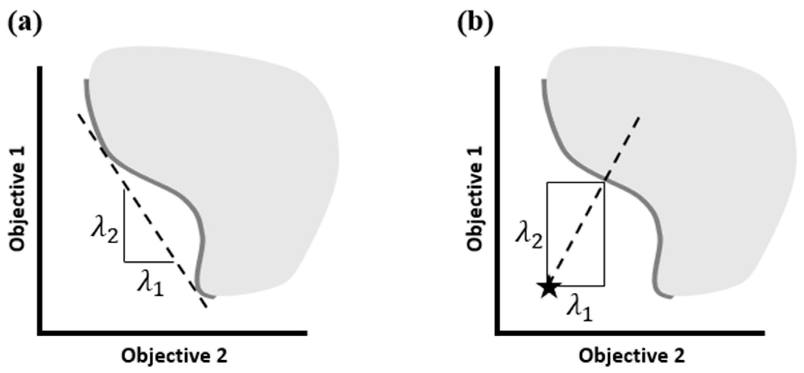
Combining preferences into one function, such that the problem can be solved with a single objective optimizer, is usually called scalarization. Consequently, the resulting function is referred to as a scalarizing function. Although the weighted sum method [66] is the most intuitive representant of this class, it has an inherent drawback in its inability to find solutions on a non-convex portion of a Pareto front (see Figure 2a). This issue is not present in methods minimizing a metric of distance to a reference point arbitrarily located in the objective space (see Figure 2b). The ASF selected for this study employs the Chebyshev metric as a measure of distance and the optimization target f T , expressing the designer’s aspirations about particular objectives, as a reference point. The scalarizing function in a multi-point formulation is defined as follows:
Y A S F M P ( x ) = m a x { λ j k ( f j k ( x ) f j k T ) } + ϱ j k λ j k ( f j k ( x ) f j k T )
Above, subscripts j and k refer to particular design conditions and objectives, respectively. The augmentation coefficient ϱ (together with the following term) guarantees proper Pareto optimality and takes an arbitrarily small positive value, here 0.05.
The coefficients λ j k serve to normalize the objective values to a similar range (Equation (24)).
λ j k = 1 f j k N f j k T
The f N is called the nadir point and represents the upper bound of an objective value. The designer usually estimates its value based on knowledge about the landscape of the objective supported by their educated judgment.
Except for the advantages referred to above and the proven efficiency, the ASF is characterized by an intuitive concept of setting a target and aiming at advancing on it.

2.2. Optimization Problem

The surrogate-based framework is applied to the I-31T aircraft air-intake duct multi-point optimization problem. The I-31T flight demonstrator is a retrofitted make of the I-23 “Manager” airplane. The plane was designed in Łukasiewicz Research Network—Institute of Aviation [67] and modified under the EU R&D program ESPOSA (Efficient Systems and Propulsion for Small Aircraft) [68]. The redesign had in scope a replacement of the piston motor with the PBS TP100 turboprop engine [69,70,71,72]. Integration of the nominally pusher-purpose engine with the tractor-type airplane required the introduction of a tailored air delivery U-shaped duct. The duct was designed by Stalewski and Żółtak [73] using a parametric design strategy [74,75] relying on the NURBS-based in-house code PARADES [76]. This study takes the outcome of the abovementioned work as an initial point and aims to further improve the duct’s performance characteristics in various flight conditions.
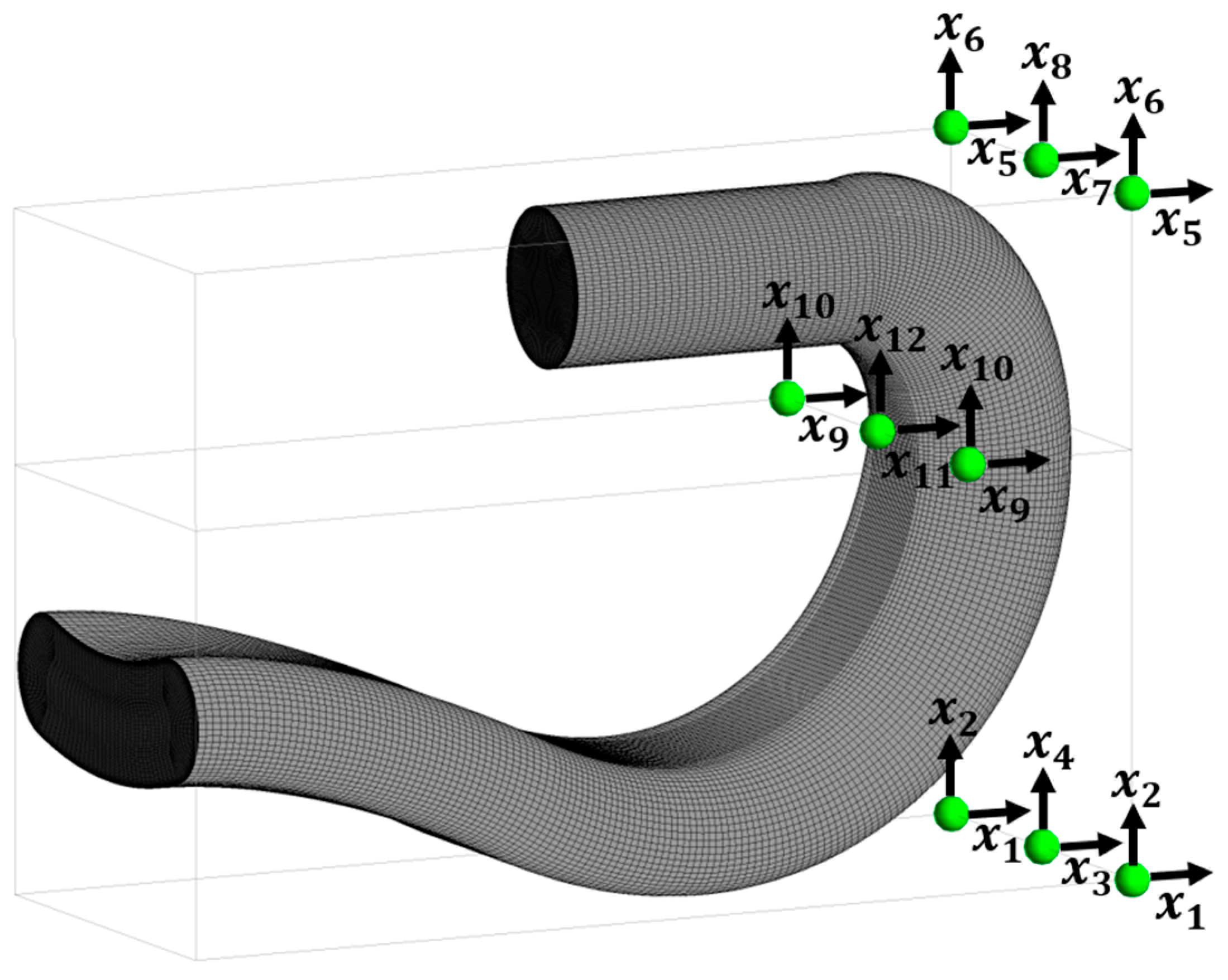
Figure 3 presents the initial air-intake duct geometry. The upstream portion of the channel is slightly S-shaped and transitions into a U-shaped duct with the flow direction. Further downstream, the U-duct interfaces with the engine compressor front face at the location marked as the Aerodynamic Interface Plane (AIP). The intake channel has a slightly converging character with a hydraulic diameter equal to 0.180 m at the duct’s entrance and 0.147 m at the AIP. The dummy extension, of a length of two diameters, is an artificial portion introduced to secure the flow solver’s stability. The duct’s inlet and AIP shapes and positions are constrained, i.e., not subject to shape deformation.
The surface of the duct in Figure 3 shows the initial computational mesh. The nine points surrounding the geometry indicate the baseline location of the mesh morpher control points subject to displacement during optimization. They are located in regions where presumed deformation should have a significant impact on the duct performance. The horizontal and vertical translation vector components form a set of design variables. Three pairs of points are bounded so that each duplet shares the exact translation. This strategy guarantees the maintenance of duct symmetry. Such a formulation results in twelve design variables, shown in Figure 3, whose ranges are defined in Table 1. The ranges corresponding to control points close to the AIP are narrower to avoid excessive deformations in the vicinity of the constrained section. Such distorted geometries would have a low probability of generating superior solutions.
The amount of pressure loss along the air intake and the level of circumferential pressure distortion at the compressor entrance substantially influence the ultimate performance and operability of the airplane engine. These two objectives are subject to minimization in the present study:
pressure   loss   coefficient :   f 1 d P = P t I N P t A I P P t I N
distortion   coefficient :   f 2 D C 60 = P t A I P min θ [ 0 , 2 π ] P t A I P ( θ π 6 , θ + π 6 ) q A I P
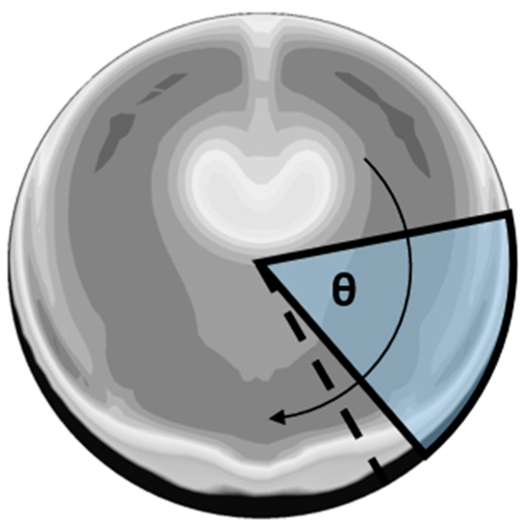
In the above equations, P t I N and P t A I P denote total pressure values mass-averaged over the inlet and AIP cross-sections, respectively, and q A I P indicates dynamic pressure mass-averaged across the AIP. The term min θ [ 0 , 2 π ] P t A I P ( θ π 6 , θ + π 6 ) refers to the lowest average pressure in the 60° sector, which is proven to have the most detrimental impact on the compressor performance [77]. This evaluation is realized by clocking a virtual sector around the AIP with Δ θ = 10 ° angular intervals—as given schematically in Figure 4.
The multi-point optimization problem considers three I-31T airplane flight conditions: DP1—nominal cruise, DP2—low-altitude climb, and DP3—high-altitude cruise. Details of the design points and related environmental properties are gathered in Table 2. The corresponding targets and nadir points are given in Table 3. The goal for the nominal cruise has a priority over the off-design conditions to reflect the contribution of this design point to the aggregated efficiency over the entire flight mission. Both performance objectives are considered to be of equal importance and share similar targets for particular design points. On the grounds of the designer’s experience, the possible falloff of 200% for each objective gives a basis for the function’s upper bound estimation.

2.3. Evaluation of Objectives

2.3.1. Flow Solver Governing Equations

The values of the objective functions are derived from the flow field solution of the air-intake duct CFD simulations. For this purpose, we use a Reynolds-averaged Navier–Stokes (RANS) solver capable of modeling three-dimensional turbulent viscous flow to accurately predict flow features characterized by a secondary flow motion, strong pressure gradients, and occurrence of separation. Such flow features are highly expected in channels of high curvature [79]. The solver is implemented using a commercial CFD code: ANSYS CFX Release 18.0.
In this study, the code solves the following Favre-averaged Navier–Stokes conservation equations:
  • The continuity equation:
ρ ¯ t + x i ( ρ ¯ u i ˜ ) = 0
  • The momentum conservation equation:
t ( ρ ¯ u i ˜ ) + x j ( ρ ¯ u i ˜ u j ˜ ) = x j ( p δ i j + t i j ¯ + ρ ¯ τ i j )
In the above formulations, ρ , u i , and p denote fluid density, velocity components, and static pressure, respectively. The tensor t i j indicates the viscous shear stress component. The operators ( · ) ¯ and ( · ) ˜ stand for the Reynolds-averaged and Favre-averaged mean variables, respectively [80]. The presence of the turbulent (Reynolds) stress tensor ρ ¯ τ i j = ρ u i u j ¯ requires additional closure for the system of RANS equations. By employing the Boussinesq hypothesis, which is the foundation of eddy viscosity-based turbulence models, the Reynolds stress tensor is approximated as:
ρ ¯ τ i j = ρ u i u j ¯ μ t ( u i ˜ x j + u j ˜ x i 2 3 u k ˜ x k δ i j ) 2 3 ρ ¯ k δ i j
where μ t is the turbulent viscosity determined using the selected turbulence model. Here, we use the two-equation SST k-ω turbulence model by Menter [81,82]. This model computes μ t from a solution of additional transport equations for two variables: the turbulent kinetic energy k and the specific dissipation rate ω (Equations (30) and (31)).
ρ t ( ρ ¯ k ) + x j ( ρ ¯ u j ˜ k ) = ρ ¯ τ i j u i ˜ x j β * ρ ¯ k ω + x j [ ( μ + σ k μ t ) k x j ]
t ( ρ ¯ ω ) + x j ( ρ ¯ u j ˜ ω ) = α ν t ρ ¯ τ i j u i ˜ x j β ρ ¯ ω 2 + x j [ ( μ + σ ω μ t ) ω x j ] + 2 ( 1 F 1 ) ρ ¯ σ ω 2 ω k x j ω x j
Details of the SST k-ω model formulation used in this paper and a specification of the closure coefficients are available in [83].
The system of transport equations is closed with the ideal gas law equation, solved for the density (Equation (32)).
p ¯ = ρ ¯ R T ˜
Here, R is the specific gas constant for air, and T is the fluid temperature. This study employs an isothermal model, for which the temperature is selected and kept constant according to the specifics of particular design points. Such an assumption is well grounded for a low Ma number flow regime and the absence of heat sources, which is accurate for the intake duct conditions.

2.3.2. Validation of Turbulence Modeling Technique

The selection of the SST k-ω turbulence model was validated prior to the optimization study. The model’s predictive quality was compared with the eddy viscosity-based k-ε turbulence model and the non-linear k-ε Explicit Algebraic Reynolds Stress Model (k-ε EARSM). All three models were considered in two options: with and without the curvature correction (CC) term. The flow field predictions for the six abovementioned models were compared with the experimental data for a benchmark U-duct provided by Azzola et al. [84,85]. Details of the validation study are available in [37].
Figure 5 groups the study results for the longitudinal (U) and circumferential (V) velocity components normalized by the bulk velocity (Ub) at the entrance to the duct’s curved portion. The k-ε turbulence model showed the most drastic underprediction in the core flow (r/D = 0) deceleration at the duct bend (see Figure 5a). Quite oppositely, the k-ε EARSM model failed to predict the circumferential flow motion at the station downstream of the curved portion. Overall, the study showed the best agreement between the flow simulations and the experimental reference data for the SST k-ω turbulence model. Moreover, no significant beneficial influence of the curvature correction term was detected. Following this reasoning, the SST k-ω model with deactivated CC term is employed in this work.

2.3.3. Details of the Flow Field Modeling Approach

Steady Navier–Stokes equations are discretized by the element-based finite volume method, with a second-order upwind approximation of convective fluxes and a second-order central representation of diffusive fluxes. An additional limiter using the Barth and Jespersen principles [86] is activated to maintain the solution’s boundedness. The solution to the equations is obtained using the coupled pressure-based algorithm iterated until the normalized residuals of the momentum and transport equations drop below 10−5.
The boundary conditions mimic the mission characteristics given in Table 2. The duct’s inlet flow conditions are defined, with the total pressure value calculated using Bernoulli’s equation for specific flight speed and altitude. Furthermore, the inlet turbulence intensity is set to T u = 10 % , and the eddy-to-molecular viscosity ratio equals ν t / ν = 100 . The amount of airflow accepted by the engine at specific design points is reflected through the mass flow rate condition at the domain outlet. The duct’s walls obey the non-slip boundary condition.
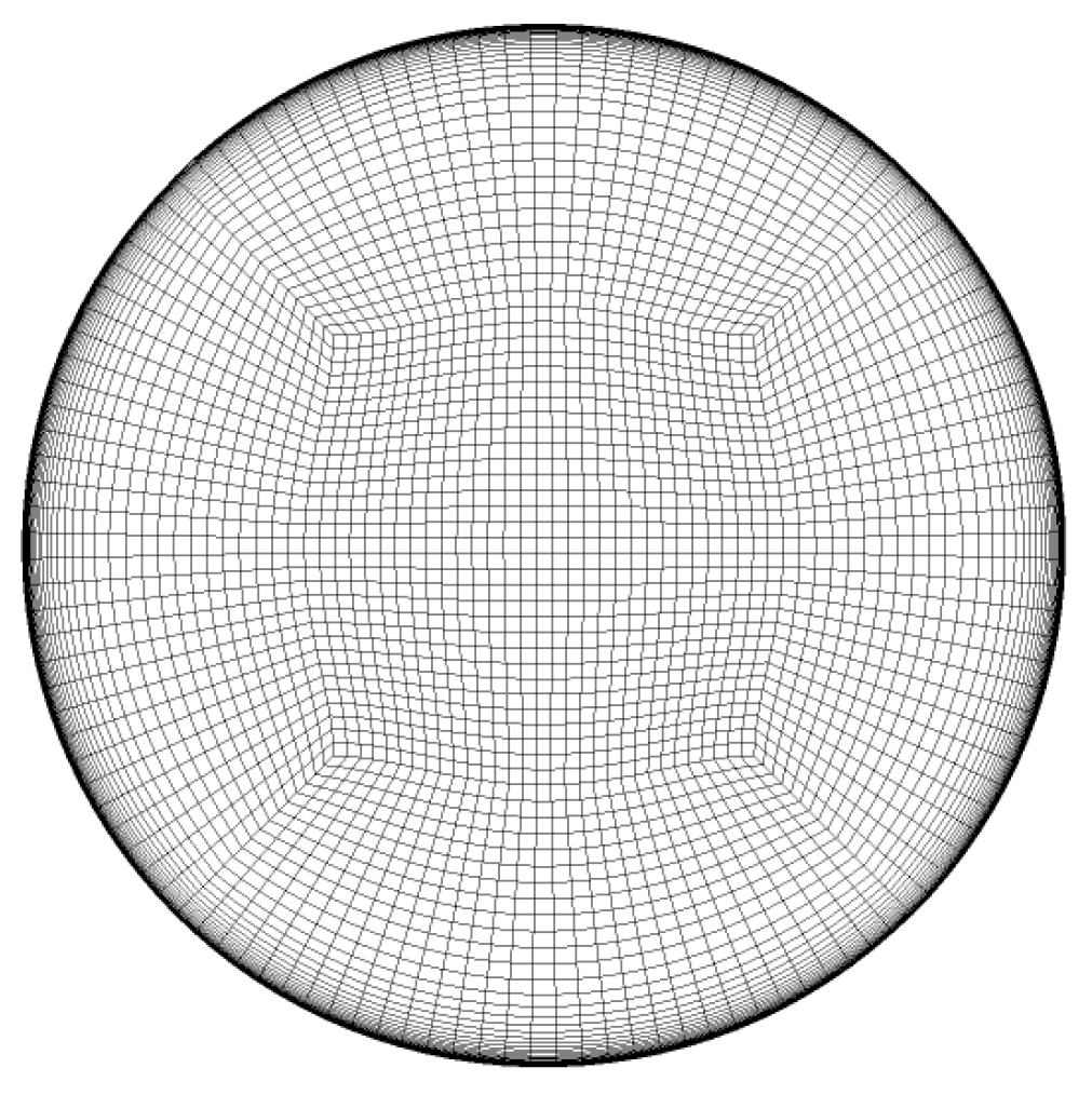
The flow domain corresponding to the duct’s interior is discretized using a structured hexahedral mesh. To secure a high-level resolution in the near-wall region accompanied by quality elements in the flow core, the mesh is built in the hybrid O-H grid topology (see Figure 6). On average, the non-dimensional wall distance is y + ~ 1.7 with extreme variation up to y + 3.5 . These values hold throughout the optimization process.
The execution of the comparative study secures the optimization results’ independence from the mesh size. Four different grid sizes are compared against the duct-wise pressure distribution. The mass-averaged total pressure values are normalized using the duct inlet pressure. The results are compared in Figure 7. The two finest grids (1,451,000 and 8,007,000 cells) show no difference in predictions for the vast majority of the duct length (~95%). A minor deviation is observable close to the duct’s outlet. Hence, the mesh with 1,451,000 elements is used as it has sufficient prediction quality and protects the computational economy of the simulations.

3. Results and Discussion

3.1. Metamodel Fit Validation

Before the optimization began, the Kriging surrogate was assessed for its ability to generalize given data, i.e., to predict objective values at unobserved locations. For this purpose, we used the leave-one-out cross-validation (LOO-CV) procedure, described in detail in Appendix A.
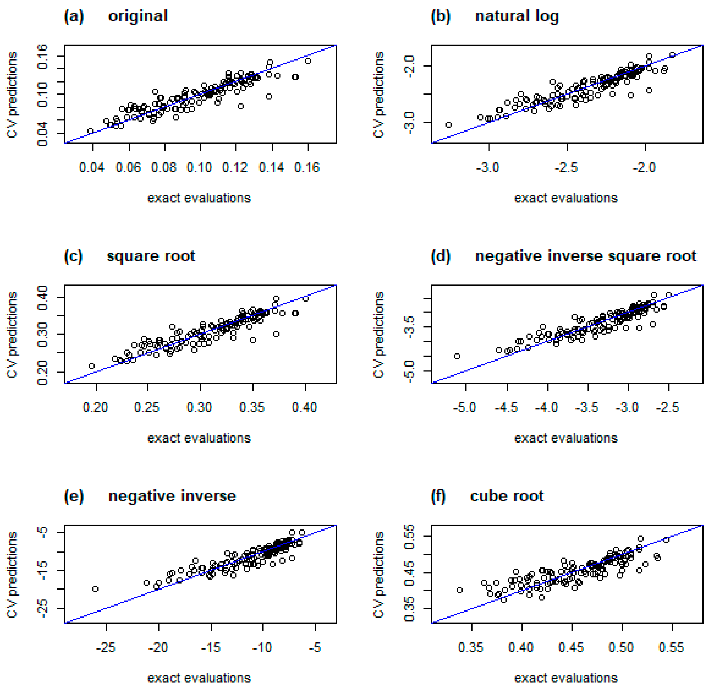
The validation process was executed for the nominal ASF formulation and its mathematical transformations given in Table 4. This action anticipates potential deficiencies in the surrogate’s prediction accuracy. In such a scenario, a deterministic mathematical function can be applied to the data set to deliberately impact its distribution and potentially improve the metamodel’s fit quality.
The outcome of the LOO-CV is presented graphically using diagnostic plots in Figure 8, Figure 9 and Figure 10. In Figure 8, values on the horizontal axis denote exact evaluations of each observation, while the vertical axis shows the surrogate prediction when the corresponding sample is omitted. The markers would be distributed perfectly on a diagonal in a utopian metamodel with zero-error predictions. A realizable high-performing surrogate would be characterized by samples located in close proximity to the imaginary line. Figure 8a shows the results for the nominal ASF. The samples approximately follow the diagonal and are reasonably distributed along the reference line. Only a few observations slightly depart from the ideal arrangement. The results for transformed data (see Figure 8b–f) present a similar pattern, with a slight tendency in some functions to cluster around the higher values (e.g., Figure 8d,e).
Figure 9 shows the distribution of the cross-validated residuals, which—as discussed in Appendix A—should be bounded in a ± 3 interval. Inspection of the residuals for nominal ASF (see Figure 9a) reveals one observation that slightly exceeds the desired limits with a residual value of ~3.5. Except for that fault, the residuals are randomly distributed along the sample values with no apparent pattern. The abovementioned deficiency does not impose a rejection of the model, although it might adversely affect its prediction accuracy. Most of the considered data transformations (see Figure 9b–e) do not remove the outlier, although the negative inverse function reduces it to the threshold value. Quite oppositely, the cube root transformation, given in Figure 9f, reduces the error variance to a healthy range without affecting randomized distribution.
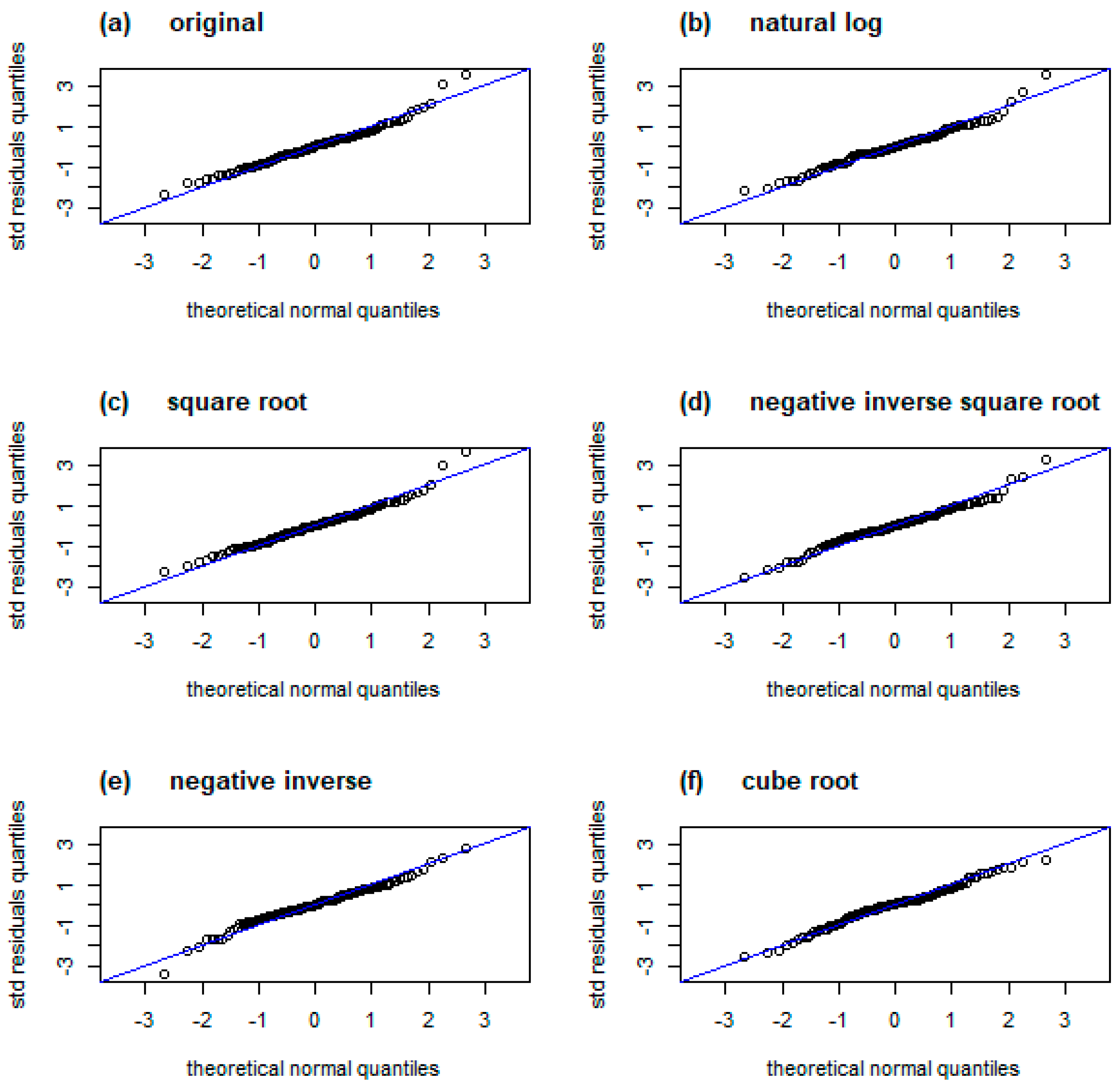
The quantile-quantile plot (Q-Q plot) in Figure 10 helps to examine the standardized residuals’ normality and homoscedasticity. The assumption of normal distribution should be satisfied for the legitimate use of MLE in the surrogate’s hyperparameter estimation. Moreover, following the Kriging principles, the residuals should be homoscedastic, i.e., the variance ought to be homogeneous across the design space [87]. The Q-Q plot draws the residuals’ quantiles sorted in ascending order (vertical axis) against the quantiles from the theoretical Gaussian distribution (horizontal axis). For normally distributed residuals, markers on the plot would follow the diagonal. A random spread of points along this line manifests residuals’ homoscedasticity.
The Q-Q plot for the original ASF (see Figure 10a) reveals that the extreme positive residuals tend to deviate counter-clockwise relative to the reference line. Such a pattern indicates that more data are located on the range’s right bound, i.e., the distribution is ‘heavy-tailed’. Moreover, the lack of a similar pattern on the left tail suggests asymmetry in the distribution with a tendency to right-skewness. Inspection of the remaining Q-Q plots reveals that only two transformations, negative inverse square root (Figure 10d) and cube root (Figure 10f), normalize the distribution of the standardized residuals.
As the cube root transformation is superior in the normalization of residuals and maintains the error variance in a healthy span, we use it to transform the ASF in further studies. Moreover, this transformation is insensitive to the sign of input, which supports the robustness of the process. Although this is an optimistic scenario, the ASF formulation potentially produces negative values for solutions superior to the presumed target. Although less popular than other considered transformations, the cube root has been recognized in applications for long-tailed data [88].

3.2. Sensitivity Analysis

A sensitivity analysis was executed to assess how strong is the dependence of the surrogate’s output (i.e., the objective function prediction) on variance in particular design variables. As a result, less impactful variables could be identified and removed from further consideration, thus reducing the computational cost of the optimization.
We used Functional Analysis of Variance (FANOVA), described in detail in Appendix B. This method assesses the contribution of particular inputs and interactions between them using the notion of Sobol’ indices [89,90]. FANOVA is particularly beneficial in use with surrogates that might be non-linear and non-monotonic but are inexpensive in the output estimation.
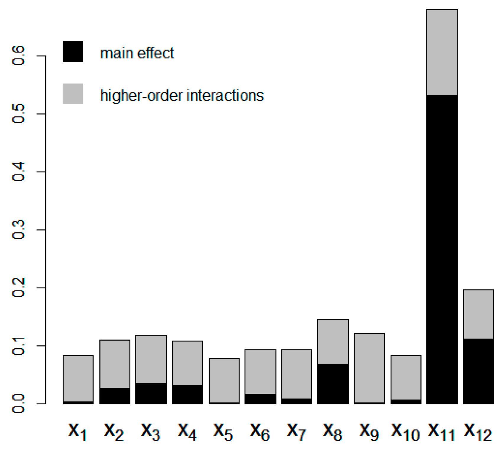
Figure 11 displays graphically the outcome of the FANOVA analysis applied to the Kriging surrogate constructed on the DoE observations. The height of the bars represents the value of the total effect Sobol’ indices, while black and gray bars’ fractions denote the main effect and aggregated higher-order interactions, respectively.
Undoubtedly, the design variable x 11 has the most substantial influence on variance in the objective function. The second most impactful is the variable x 12 . Both factors correspond to the spatial motion of the control point located in the duct’s inner wall area (see Figure 3). Except for the high total index value, these variables are characterized by a strong direct effect, suggesting their crucial influence on the final optimization results.
Quite oppositely, the impact of variables { x 1 , x 5 , x 7 ,   x 10 } is less significant. Their already low total effect value is related mainly to the higher-order interactions rather than to the direct impact. For this reason, these variables are removed from the design space, notably reducing its dimensions and increasing the process’s cost-efficiency. Variable x 6 presents a similar level of total impact to x 7 , although its main influence is slightly more prominent. Contrarily, the direct effect of x 9 is minor; however, strong higher-order interactions result in a meaningful value of the total effect index. It depends on the designer’s intuition whether such variables should be further considered; here, we preserve them in the study.

3.3. Assessment of Deformed Mesh Quality

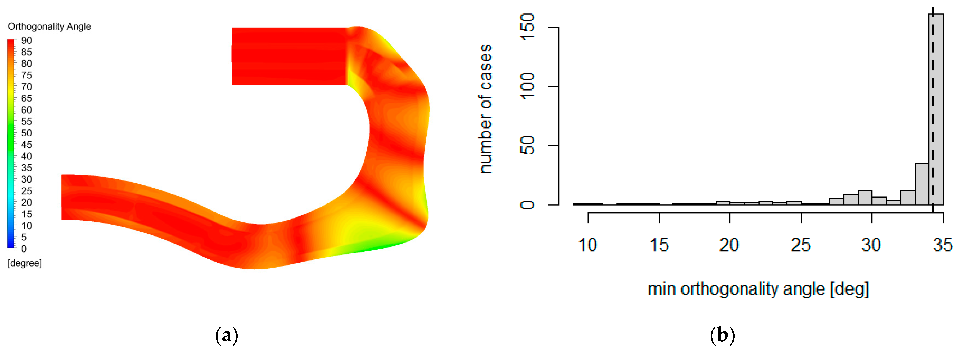
This section discusses the influence of shape deformation on the mesh quality using the metric defined in Section 2.1.2. Figure 12a displays the mesh orthogonality angle distribution plotted on a symmetry plane of selected exceptionally deformed duct geometry. Although a fall in the quality criterion is evident in the strongly warped regions, the bulk values are well above the warning limit of 20°.
Figure 12b shows a histogram of the minimum value of the orthogonality angle for all solutions produced in the course of optimization. The dashed line denotes the metric’s reference value for the baseline geometry. The bulk of generated solutions maintain the quality criterion value close to the reference level. Some cases, however, report a reduction in the orthogonality angle, yet still without violating the warning limit. Finally, a few solutions show criterion values below 20°. Such distortion in the mesh elements might trigger a warning for the flow solver. After inspection, the cases were identified as excessively deformed and, as such, located far from the objective target. These instances did not harm the solver’s stability and convergence; hence, they were accepted.

3.4. Optimization Results

Figure 13 shows the contours of the baseline and optimized shape displayed on the duct’s symmetry cross-section. The optimization affects the geometry mostly in the transition from the channel to the AIP. The sharp shape change from the inner wall to the compressor entrance is moderated in the final solution. Moreover, the optimizer reduced the curvature of the inner and outer walls; however, the effect on the concave side is more apparent.
Table 5 groups the optimized objective function values for all considered conditions and compares them with the reference levels. The results are presented on an absolute scale and as a percentage of improvement with respect to the baseline shape. Undoubtedly, the optimizer was successful in finding a solution that improves both objectives for all considered design points.
The greatest improvement level in both objectives is attained for the nominal cruise, which corresponds with the predefined preferences in targets (see Table 3). Furthermore, comparable gains in the pressure loss and the distortion coefficient coincide with the equality in targets set for both objectives. However, a slight consistent preference towards refinement in the distortion coefficient is noticeable. Such an outcome confirms the ability of the ASF formulation to guide optimization toward the presumed target, although a margin has to be considered for potential moderate departures.
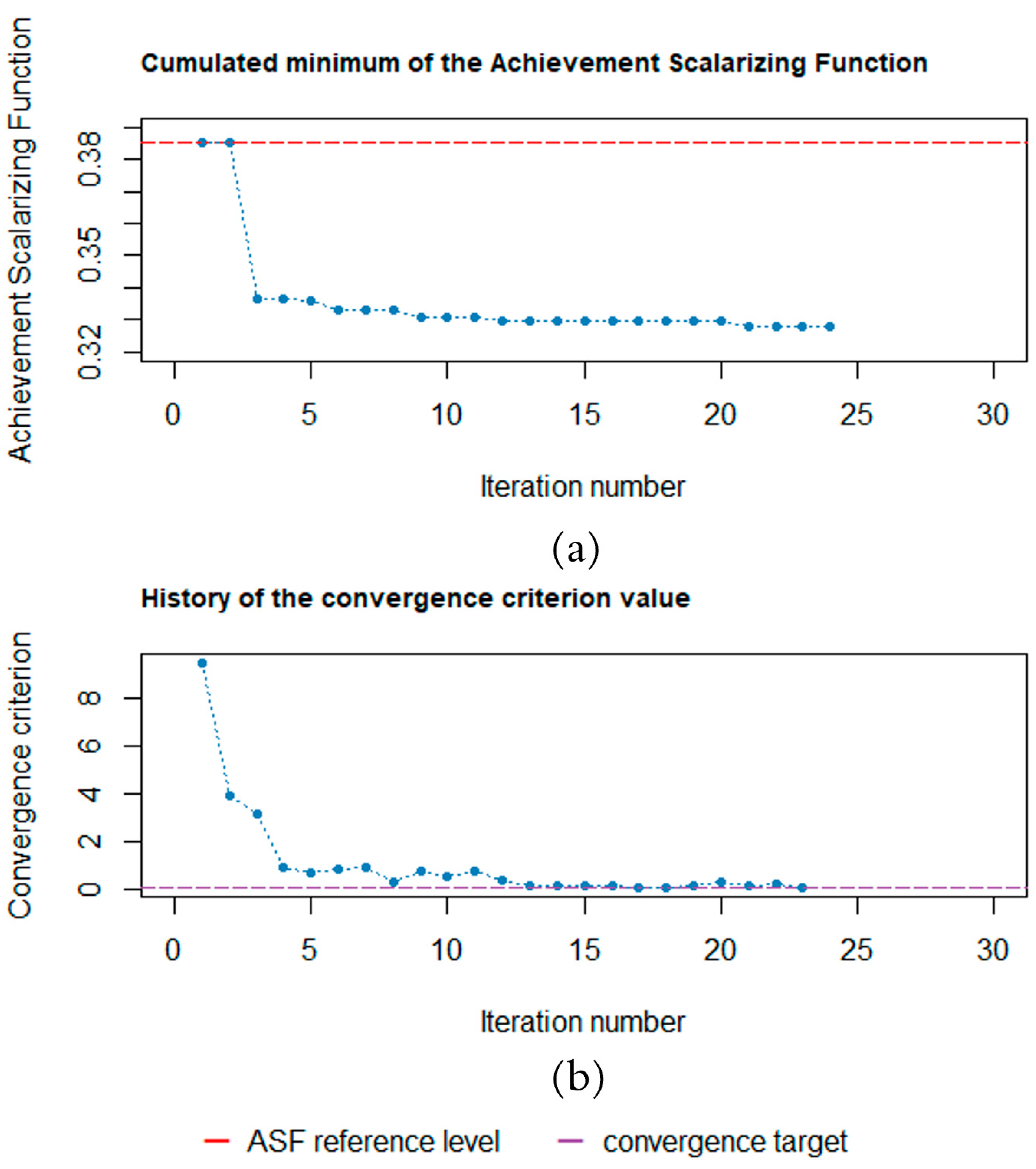
Figure 14 shows a cumulated best value of the ASF and the convergence criterion value along the EGO steps. A rapid convergence towards the optimized solutions is evident. The optimizer finds a case significantly improving the initial ASF value (marked by the dashed red line) already in the first iteration. Such superior performance results from a fine design space sampling and high-quality surrogate fit.
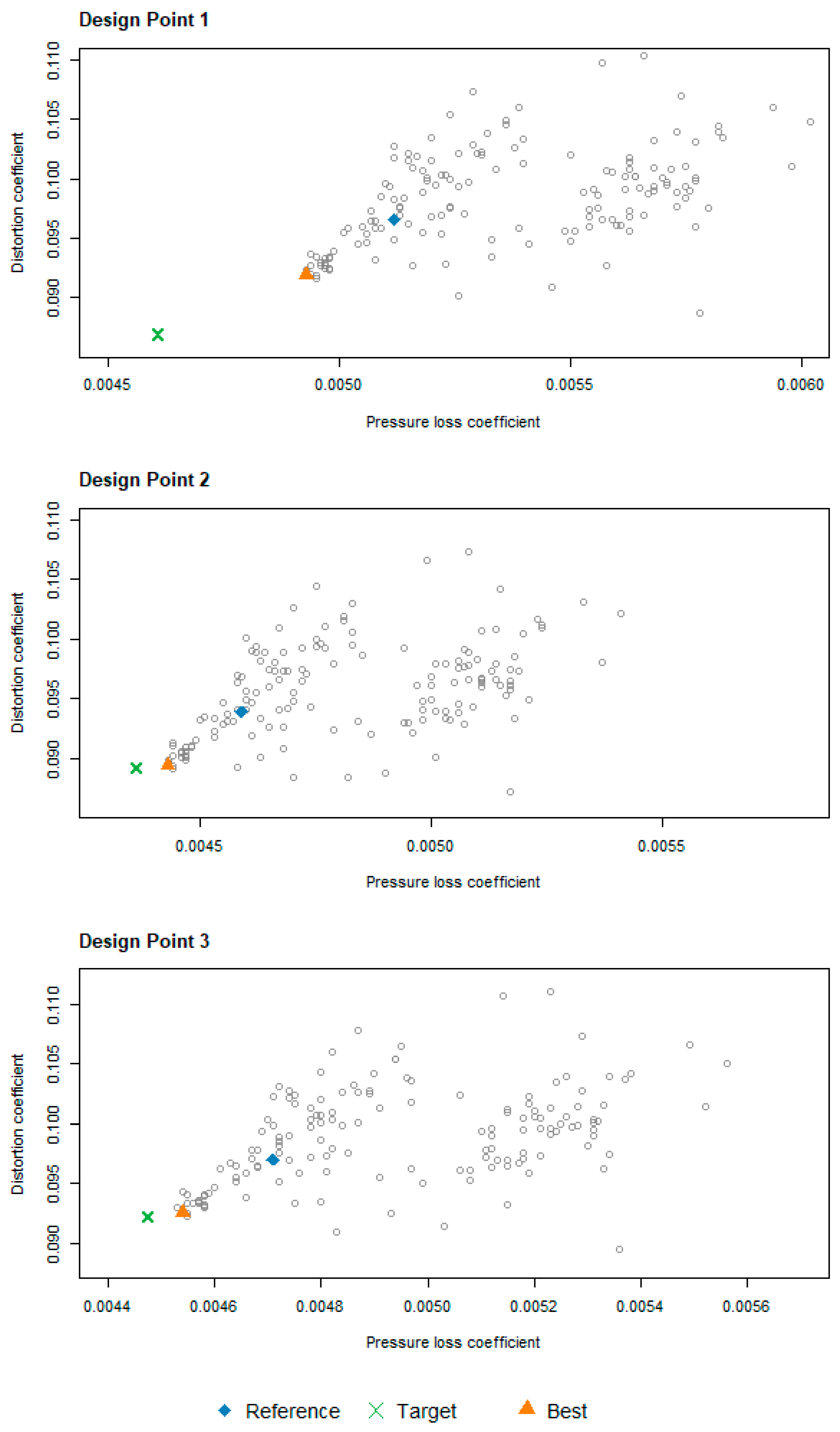
The objective space with DoE and EGO evaluations is displayed in Figure 15 for the three considered design points. For all conditions, the instances from the optimization stage converge towards an imaginary line connecting the reference and target points. The vast majority of the Pareto front is not resolved, which is intentional and prioritizes the use of computational resources in the target’s neighborhood. Such an observation shows the algorithm’s ability to follow the direction defined by a predetermined target.
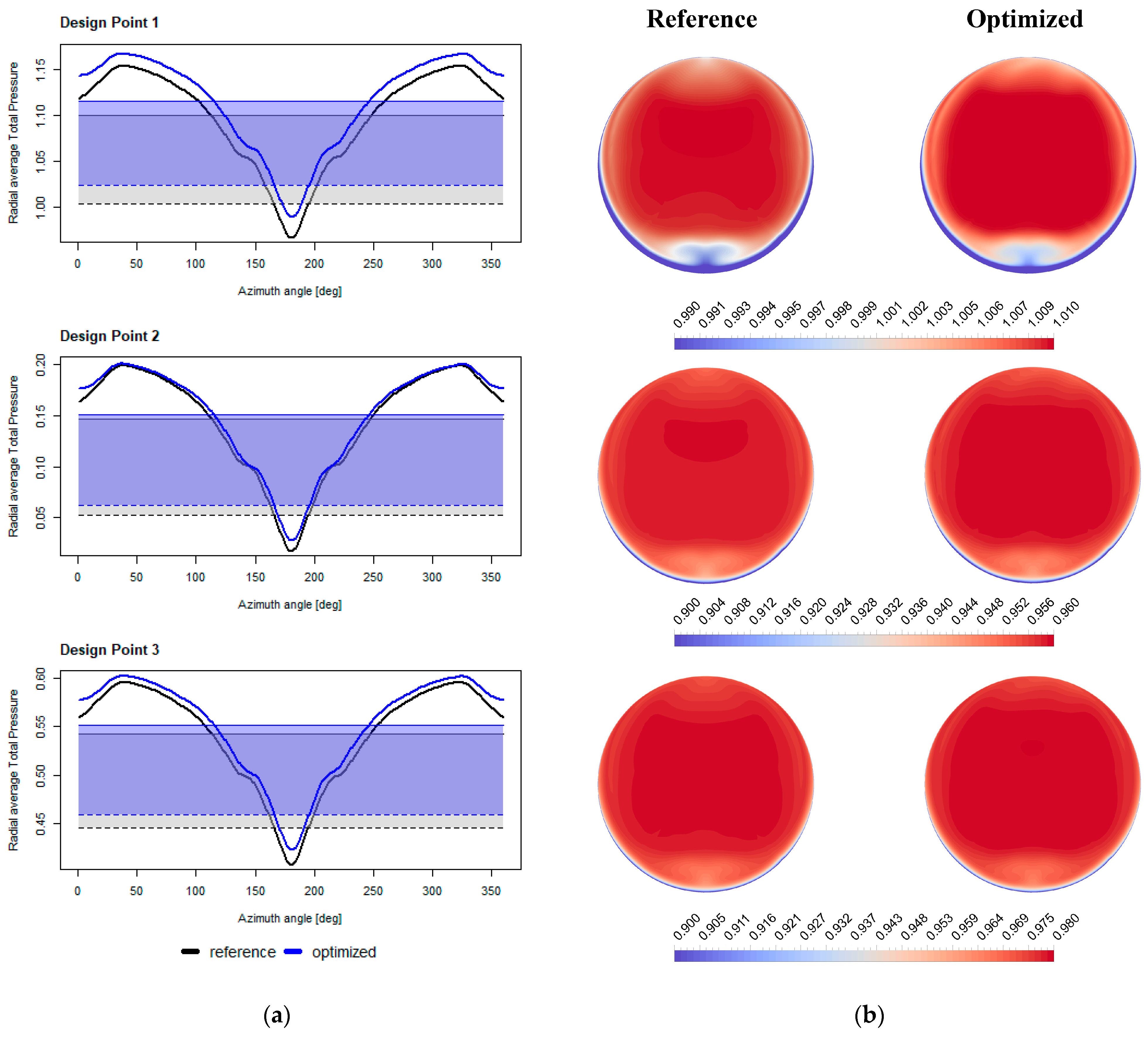
Figure 16 gives insights into the improvements in the distortion coefficient. Figure 16a contrasts radially averaged total pressure values for the reference and optimized solutions. The pressure value is normalized against the average dynamic pressure over the AIP and plotted against the azimuthal position at the compressor face. For the optimized solution, an apparent reduction in the total pressure’s lowest peak value manifests for all considered design points. The source of refinement is located in the 150–210° sector, corresponding with the transition area from the duct’s inner wall to the AIP. Such an improvement translates directly to an enhancement in the distortion coefficient. A slight shift in the total pressure curves for the optimized solution toward higher values is an effect of reduction in the duct’s pressure loss; however, it does not directly impact the distortion metric.
The distortion coefficient value can be visualized intuitively as an area between a plane-averaged total pressure (solid lines in Figure 16a) and total pressure averaged over the worst 60° sector (dashed lines in Figure 16a). The areas are marked with shaded fields with a color corresponding to the reference (gray) and optimized (blue) solutions. The area of the fields representing the improved solution is visibly smaller than the corresponding regions for the baseline case. Such an observation confirms the quantitative results given above in Table 5.
Figure 16b groups the maps of total pressure normalized by the average dynamic head and plotted at the AIP. The pressure field homogenization is visible for all conditions, although the most significant effect is noticeable for Design Point 1. This corresponds with the highest D C 60 improvement observed in the quantitative data. The reduction in the low-pressure zone visible in the six o’clock position matches the improvement in the 150–210° sector discussed above. A slight improvement is observable in the twelve o’clock region corresponding to the convex wall transition to the AIP. This local enhancement can also be seen in Figure 16a for sector ~360 ± 30°. Even though such improvement does not influence the distortion metric, an increase in the pressure field uniformity at the compressor face is a positive effect.
Figure 17 shows details of the flow field with regard to the pressure loss coefficient improvements. Figure 17a displays the flow loss evolution along the duct through a local pressure loss coefficient contour. This metric is conceptually similar to the pressure loss objective; however, it quantifies the drop from the duct’s inlet to each spatial location (Equation (33)).
d P * = P t I N P t P t I N
The most apparent enhancement is the reduction in pressure loss in the transition region from the duct’s convex wall to the AIP. Adjusting the shape of the wall’s top sector and the above-discussed reduction in the low-pressure zone on the concave side transition removes a secondary flow motion downstream of the AIP. This improvement is visualized in Figure 17b, in which the vertical velocity component values color flow streamlines. The two counter-rotating vortices, visible at the twelve o’clock position in the baseline case, are evidently removed in the optimized solution.
The reduction in the concave wall curvature and expansion of the duct’s cross-section results in a diffusing shape, bringing additional pressure recovery from the flow kinetic energy. This effect is subtle but still contributes to the duct’s overall performance.

4. Conclusions

The proposed aerodynamic optimization framework, constructed from state-of-the-art components in advanced surrogates, mesh morphing, and distance-based scalarization, was applied to the multi-point optimization problem of an I-31T airplane air-intake duct. The study aimed to simultaneously improve the duct’s pressure loss and flow distortion under three flight conditions: nominal cruise, low-altitude climbing, and high-altitude cruise.
The optimizer obtained both objective values superior to the reference configuration for all considered design points. The consistent level of improvements in the pressure loss and flow distortion confirms the capacity of the ASF-based formulation to guide optimization toward the presumed target. The study results prove the methodology’s potential for optimizing complex multi-objective air-intake duct problems in multiple flight conditions while saving substantial computational resources.
Moreover, FANOVA-based sensitivity analysis was recognized as a valuable tool for assessing the importance of particular design variables. Application of this technique is particularly beneficial in Kriging-based frameworks where the use of surrogate predictions balances high computational costs related to the variance-based techniques.
This research, however, may be subject to potential limitations regarding the generalization of its results. Primarily, the number of design variables was relatively moderate, which favors the use of the Kriging surrogate. Although literature sources report a considerable margin for increased design space dimensions, studies on larger problems should be executed to prove the framework’s efficiency. Moreover, the results revealed that all considered flight conditions were coherent in the direction of shape improvements. Although justified for this particular application, this scenario might only represent part of the class of problems. Future studies should cover scenarios with design points of contradicting performance requirements to generalize the results. Finally, the optimization was initiated from an already well-designed solution, which aimed to set an ambitious task for the optimizer but also resulted in a relatively low level of required deformations. Optimization studies demanding significant geometry adjustments may be subject to numerical errors resulting from an excessively distorted mesh. Such problems may require the implementation of a solution for handling erroneous data samples.
Optimization studies using the proposed framework could be expanded to more holistic multi-disciplinary problems. The most natural development would include solid body mechanics addressing the structural targets, although involvement of the intuitively more distant performance and economic objectives seems feasible. No fundamental reasons were identified that might inhibit the ASF-based formulation in handling such heterogeneous goals, although this would need to be proved in further studies.

Author Contributions

Conceptualization, P.S.D., S.K. and J.Ż.; methodology, P.S.D. and S.K.; software, P.S.D.; validation, P.S.D.; formal analysis, P.S.D.; investigation, P.S.D.; resources, P.S.D. and J.Ż.; data curation, P.S.D.; writing—original draft preparation, P.S.D.; writing—review and editing, P.S.D. and S.K.; visualization, P.S.D.; supervision, P.S.D., S.K. and J.Ż. All authors have read and agreed to the published version of the manuscript.

Funding

This work was co-funded by the Ministry of Education and Science as part of the “Implementation Doctorate first edition” program under the agreement no 3/DW/2017/01/1.

Data Availability Statement

Not applicable.

Acknowledgments

We would like to express our great appreciation to Karolina Drężek for her support in the preparation of figures.

Conflicts of Interest

The authors declare no conflict of interest. The funders had no role in the design of the study; in the collection, analyses, or interpretation of data; in the writing of the manuscript; or in the decision to publish the results.

Appendix A. Leave-One-Out Cross-Validation

The leave-one-out cross-validation (LOO-CV) technique [91] sequentially omits one sample from the set of N observations, and the metamodel is constructed from the remaining N 1 points. Afterward, the objective is predicted at the left-out sample’s location, and the estimated value is compared with the known evaluation. The concept of LOO-CV is demonstrated schematically in Figure A1. The operation repeats N times, resulting in an assessment of prediction accuracy for the whole observation set.
Figure A1. Schematic representation of LOO-CV concept for one-dimensional design space.
Aerospace 10 00266 g0a1
The measure of difference between the true objective value y ( x i ) and the corresponding LOO-CV prediction y ^ D i ( x i ) is termed a residual (Equation (A1)).
ϵ i = y ( x i ) y ^ D i ( x i )
The residuals are standardized using the variance estimator s D i 2 ^ ( x i ) available in the Kriging surrogate (Equation (A2)).
ϵ i z = ϵ i s D i 2 ^
If the residuals approximately follow the Gaussian distribution, the objective evaluation locates within three standard deviations from the predicted Kriging mean with a confidence level of 99.7%. Thus, a surrogate with good prediction quality should be characterized by standardized residuals bounded in a ±3 interval [23]. The probability of a residual being further away is less than 0.3%. Detecting such an outlier may suggest poor prediction quality in the vicinity of the corresponding observation.

Appendix B. Functional Analysis of Variance (FANOVA)

Consider that the design space X forms a p -dimensional hypercube and x X is a vector of independent random variables normalized to a range [ 0 , 1 ] . The surrogate model is described by a square-integrable function Y = f ( x ) defined in X , which can be decomposed using the FANOVA representation [89]:
Y ( x ) = f 0 + i = 1 p f i ( x i ) + 1 i < j p f i j ( x i , x j ) + + f 1 , , p ( x 1 , , x p )
In the above equation, the centered and orthogonal terms denote:
mean   value   f 0 = E [ Y ( x ) ]
main   effects   f i ( x i ) = E [ Y ( x ) | x i ] f 0
second - order   interactions   f i j ( x i , x j ) = E [ Y ( x ) | x i , x j ] f 0 f i ( x i ) f j ( x j )
The interactions of higher orders can be constructed accordingly as conditional expected values.
A similar technique serves for a decomposition of the model output’s variance:
V a r ( Y ( x ) ) = i = 1 p V a r ( f i ( x i ) ) + 1 i < j p V a r ( f i j ( x i , x j ) ) + + V a r ( f 1 , , p ( x 1 , , x p ) )
The individual contribution of variable x i to the variance in the model’s output is quantified by the main effect Sobol index:
S i = V a r ( f i ( x i ) ) V a r ( Y ( x ) )
The influence of interaction between any two variables x i and x j is described by the second-order Sobol’ index:
S i j = V a r ( f i j ( x i , x j ) ) V a r ( Y ( x ) )
All higher-order interactions can be assessed by Sobol’ indices, constructed following a similar concept of ratios between decomposed higher-order terms and the overall output variance. The values of main and higher-order indices for all variables sum to unity (Equation (A10)).
i = 1 p S i + 1 i < j p S i j + + S 1 , , p = 1
The aggregated contribution to the model’s output variance of the i -th variable is measured by the total effect Sobol’ index:
S i T = E [ V a r ( Y ( x ) | x \ { x i } ) ] V a r ( Y ( x ) )
In practice, only main and total indices are assessed for economic reasons. Knowing them allows for an estimation of the combined influence of all-order interactions.
The values of the Sobol’ indices are to be computed numerically. For this purpose, this study employs the FAST algorithm [92] available in the R package sensitivity [93].

References

  1. Airbus. Global Market Forecast 2022–2041. Available online: https://www.airbus.com/en/products-services/commercial-aircraft/market/global-market-forecast (accessed on 16 January 2023).
  2. Boeing. Boeing Commercial Market Outlook 2022–2041. Available online: https://www.boeing.com/resources/boeingdotcom/market/assets/downloads/CMO_2022_Report_FINAL_v02.pdf (accessed on 16 January 2023).
  3. European Commission Website. A European Green Deal-Striving to be the First Climate-Neutral Continent. Available online: https://ec.europa.eu/info/strategy/priorities-2019-2024/european-green-deal_en (accessed on 16 January 2023).
  4. Furlan, F.; Chiereghin, N.; Kipouros, T.; Benini, E.; Savill, M. Computational design of S-Duct intakes for distributed propulsion. Aircr. Eng. Aerosp. Technol. 2014, 86, 473–777. [Google Scholar] [CrossRef]
  5. Goldberg, D.E. Genetic Algorithms in Search, Optimization, and Machine Learning; Addison Wesley: Reading, UK, 1989. [Google Scholar]
  6. D’Ambros, A.; Kipouros, T.; Zachos, P.; Savill, M.; Benini, E. Computational Design Optimization for S-Ducts. Designs 2018, 2, 36. [Google Scholar] [CrossRef] [Green Version]
  7. Zeng, L.; Pan, D.; Ye, S.; Shao, X. A fast multiobjective optimization approach to S-duct scoop inlets design with both inflow and outflow. Proc. Inst. Mech. Eng. Part G J. Aerosp. Eng. 2019, 233, 3381–3394. [Google Scholar] [CrossRef]
  8. Sharma, M.; Baloni, B.D. Design optimization of S-shaped compressor transition duct using particle swarm optimization algorithm. SN Appl. Sci. 2020, 2, 221. [Google Scholar] [CrossRef] [Green Version]
  9. Kennedy, J. Particle Swarm Optimization. In Encyclopedia of Machine Learning; Sammut, C., Webb, G.I., Eds.; Springer: Boston, MA, USA, 2011; pp. 760–766. [Google Scholar] [CrossRef]
  10. Wang, G.G.; Shan, S. Review of Metamodeling Techniques in Support of Engineering Design Optimization. J. Mech. Des. 2007, 129, 370–380. [Google Scholar] [CrossRef]
  11. Simpson, T.W.; Poplinski, J.D.; Koch, P.N.; Allen, J.K. Metamodels for Computer-based Engineering Design: Survey and recommendations. Eng. Comput. 2001, 17, 129–150. [Google Scholar] [CrossRef] [Green Version]
  12. Han, Z.-H.; Zhang, K.-S. Surrogate-Based Optimization. In Real-World Applications of Genetic Algorithms; Roeva, O., Ed.; InTech: London, UK, 2012; pp. 343–362. [Google Scholar]
  13. Skinner, S.N. State-of-the-art in aerodynamic shape optimisation methods. Appl. Soft Comput. J. 2018, 62, 933–962. [Google Scholar] [CrossRef]
  14. Forrester, A.I.J.; Keane, A.J. Recent advances in surrogate-based optimization. Prog. Aerosp. Sci. 2009 45, 50–79. [CrossRef]
  15. Snyman, J.A.; Wilke, D.N. Practical Mathematical Optimization–Basic Optimization Theory and Gradient-Based Algorithms, 2nd ed.; Springer: Cham, Switzerland, 2018. [Google Scholar]
  16. Khuri, A.I.; Mukhopadhyay, S. Response surface methodology. WIREs Comp. Stat. 2010, 2, 128–149. [Google Scholar] [CrossRef]
  17. Friedman, J.H. Multivariate Adaptive Regression Splines. Ann. Stat. 1991, 19, 1–67. [Google Scholar] [CrossRef]
  18. Regis, R.G.; Shoemaker, C.A. Constrained Global Optimization of Expensive Black Box Functions Using Radial Basis Functions. J. Glob. Optim. 2005, 31, 153–171. [Google Scholar] [CrossRef]
  19. Haykin, S. Neural Networks: A Comprehensive Foundation, 3rd ed.; Pearson Prentice Hall: Upper Saddle River, NJ, USA, 2007. [Google Scholar]
  20. Krige, D.G. A Statistical Approach to Some Basic Mine Valuation Problems on the Witwatersrand. J. Chem. Metall. Soc. S. Min. Afr. 1951, 52, 119–139. [Google Scholar] [CrossRef]
  21. Matheron, G. Principles of geostatistics. Econ. Geol. 1963, 58, 1246–1266. [Google Scholar] [CrossRef]
  22. Sacks, J.; Welch, W.J.; Mitchell, J.S.B.; Henry, P.W. Design and Experiments of Computer Experiments. Stat. Sci. 1989, 4, 409–423. [Google Scholar] [CrossRef]
  23. Jones, D.R.; Schonlau, M.; Welch, W.J. Efficient Global Optimization of Expensive Black-Box Functions. J. Glob. Optim. 1998, 13, 455–492. [Google Scholar] [CrossRef]
  24. Lu, H.; Zheng, X.; Li, Q. A combinatorial optimization design method applied to S-shaped compressor transition duct design. Proc. Inst. Mech. Eng. Part G J. Aerosp. Eng. 2014, 228, 1749–1758. [Google Scholar] [CrossRef]
  25. Immonen, E. Shape optimization of annular S-ducts by CFD and high-order polynomial response surfaces. Eng. Comput. 2018, 35, 932–954. [Google Scholar] [CrossRef]
  26. Gan, W.; Zhang, X. Design optimization of a three-dimensional diffusing S-duct using a modified SST turbulent model. Aerosp. Sci. Technol. 2017, 63, 63–72. [Google Scholar] [CrossRef]
  27. Jin, D.; Liu, X.; Zhao, W.; Gui, X. Optimization of endwall contouring in axial compressor S-shaped ducts. Chin. J. Aeronaut. 2015, 28, 1076–1086. [Google Scholar] [CrossRef] [Green Version]
  28. Zerbinati, A.; Désidéri, J.A.; Duvigneau, R. Application of metamodel-assisted Multiple-Gradient Descent Algorithm (MGDA) to air-cooling duct shape optimization. In Proceedings of the ECCOMAS—European Congress on Computational Methods in Applied Sciences and Engineering-2012, Vienna, Austria, 10–14 September 2012. [Google Scholar]
  29. Verstraete, T.; Coletti, F.; Bulle, J.; Vanderwielen, T.; Arts, T. Optimization of a U-Bend for Minimal Pressure Loss in Internal Cooling Channels: Part I—Numerical Method. ASME J. Turbomach. 2013, 135, 051015. [Google Scholar] [CrossRef]
  30. Storn, R.; Price, K. Differential Evolution—A Simple and Efficient Heuristic for Global Optimization over Continuous Spaces. J. Glob. Optim. 1997, 11, 341–359. [Google Scholar] [CrossRef]
  31. Verstraete, T.; Li, J. Multi-Objective Optimization of a U-Bend for Minimal Pressure Loss and Maximal Heat Transfer Performance in Internal Cooling Channels. In Proceedings of the ASME Turbo Expo 2013: Turbine Technical Conference and Exposition Volume 3A: Heat Transfer, San Antonio, TX, USA, 3–7 June 2013. [Google Scholar] [CrossRef]
  32. Koo, G.-W.; Lee, S.-M.; Kim, K.-Y. Shape optimization of inlet part of a printed circuit heat exchanger using surrogate modeling. Appl. Therm. Eng. 2014, 72, 90–96. [Google Scholar] [CrossRef]
  33. Wang, B.; Wang, Q. Numerical Optimization of Electromagnetic Performance and Aerodynamic Performance for Subsonic S-Duct Intake. Aerospace 2022, 9, 665. [Google Scholar] [CrossRef]
  34. Bae, H.; Park, S.; Kwon, J. Efficient global optimization for S-duct diffuser shape design. Proc. Inst. Mech. Eng. Part G J. Aerosp. Eng. 2013, 227, 1516–1532. [Google Scholar] [CrossRef]
  35. Dehghani, M.; Ajam, H.; Farahat, S. Automated Diffuser Shape Optimization based on CFD Simulations and Surrogate Modeling. J. Appl. Fluid Mech. 2016, 9, 2527–2535. [Google Scholar] [CrossRef]
  36. Marchlewski, K.; Łaniewski-Wołłk, Ł.; Kubacki, S. Aerodynamic Shape Optimization of a Gas Turbine Engine Air-Delivery Duct. J. Aerosp. Eng. 2020, 33, 04020042. [Google Scholar] [CrossRef]
  37. Drężek, P.S.; Kubacki, S.; Żółtak, J. Multi-objective surrogate model-based optimization of a small aircraft engine air-intake duct. Proc. Inst. Mech. Eng. Part G J. Aerosp. Eng. 2022, 236, 2909–2921. [Google Scholar] [CrossRef]
  38. Nikulin, Y.; Miettinen, K.; Mäkelä, M.M. A new achievement scalarizing function based on parameterization in multiobjective optimization. OR Spectr. 2012, 34, 69–87. [Google Scholar] [CrossRef] [Green Version]
  39. Biancolini, M.E.; Costa, E.; Cella, U.; Groth, C.; Veble, G.; Andrejašič, M. Glider fuselage-wing junction optimization using CFD and RBF mesh morphing. Aircr. Eng. Aerosp. Technol. 2016, 88, 740–752. [Google Scholar] [CrossRef]
  40. Kapsoulis, D.; Asouti, V.; Giannakoglou, K.; Porziani, S.; Costa, E.; Groth, C.; Cella, U.; Biancolini, M.V. Evolutionary aerodynamic shape optimization through the RBF4AERO platform. In Proceedings of the VII European Congress on Computational Methods in Applied Sciences and Engineering (ECCOMAS Congress 2016) Crete, Greece, 5–10 June 2016; Institute of Structural Analysis and Antiseismic Research, School of Civil Engineering, National Technical University of Athens (NTUA): Athens, Greece; pp. 4146–4155. [CrossRef]
  41. Savastano, W.; Pranzitelli, A.; Andrews, G.E.; Biancolini, M.E.; Ingham, D.B.; Pourkashanian, M. Goal Driven Shape Optimisation for Conjugate Heat Transfer in an Effusion Cooling Plate. In Proceedings of the ASME Turbo Expo 2015: Turbine Technical Conference and Exposition, Montreal, Quebec, Canada, 15–19 June 2015; The American Society of Mechanical Engineers: New York, NY, USA, 2015; Volume 5A: Heat Transfer. [Google Scholar] [CrossRef] [Green Version]
  42. Mastrippolito, F.; Aubert, S.; Ducros, F.; Buisson, M. RBF-based mesh morphing improvement using Schur complement ap-plied to rib shape optimization. Int. J. Numer. Methods Heat Fluid Flow 2020, 30, 4241–4257. [Google Scholar] [CrossRef]
  43. Brahmachary, S.; Fujio, C.; Aksay, M.; Ogawa, H. Design optimization and off-design performance analysis of axisymmetric scramjet intakes for ascent flight. Phys. Fluids 2022, 34, 036109. [Google Scholar] [CrossRef]
  44. Brahmachary, S.; Fujio, C.; Ogawa, H. Multi-point design optimization of a high-performance intake for scramjet-powered ascent flight. Aerosp. Sci. Technol. 2020, 107, 106362. [Google Scholar] [CrossRef]
  45. Fujio, C.; Ogawa, H. Physical insights into multi-point global optimum design of scramjet intakes for ascent flight. Acta Astronaut. 2022, 194, 59–75. [Google Scholar] [CrossRef]
  46. Chiang, C.; Koo, D.; Zingg, D.W. Aerodynamic Shape Optimization of an S-Duct Intake for a Boundary-Layer Ingesting Engine. J. Aircr. 2022, 59, 725–741. [Google Scholar] [CrossRef]
  47. Park, J.-S.; Baek, J. Efficient computation of maximum likelihood estimators in a spatial linear model with power exponential covariogram. Comput. Geosci. 2001, 27, 1–7. [Google Scholar] [CrossRef]
  48. Roustant, O.; Ginsbourger, D.; Deville, Y. DiceKriging, DiceOptim: Two R Packages for the Analysis of Computer Experiments by Kriging-Based Metamodeling and Optimization. J. Stat. Softw. 2012, 51, 1–55. [Google Scholar] [CrossRef] [Green Version]
  49. Liu, H.; Ong, Y.-S.; Cai, J. A survey of adaptive sampling for global metamodeling in support of simulation-based complex engineering design. Struct. Multidiscip. Optim. 2018, 57, 393–416. [Google Scholar] [CrossRef]
  50. McKay, M.D.; Beckman, R.J.; Conover, W.J. A Comparison of three methods for selecting values of input variables in the analysis of output from a computer code. Technometrics 1979, 21, 239–245. [Google Scholar] [CrossRef]
  51. Viana, F.A.C. Things You Wanted to Know About the Latin Hypercube Design and Were Afraid to Ask. In Proceedings of the 10th World Congress on Structural and Multidisciplinary Optimization, Orlando, FL, USA, 19–24 May 2013. [Google Scholar]
  52. Crombecq, K.; Couckuyt, I.; Gorissen, D.; Dhaene, T. Space-Filling Sequential Design Strategies for Adaptive Surrogate Modelling. In The First International Conference on Soft Computing Technology in Civil, Structural and Environmental Engineering, Funchal Madeira, Portugal, 1–4 September 2009; Civil-Comp Press: Stirlingshire, UK, 2009. [Google Scholar] [CrossRef]
  53. Liefvendahl, M.; Stocki, R. A study on algorithms for optimization of Latin hypercubes. J. Stat. Plan Inference 2006, 136, 3231–3247. [Google Scholar] [CrossRef] [Green Version]
  54. Santner, T.J.; Williams, B.J.; Notz, W.I. Space-Filling Designs for Computer Experiments. In The Design and Analysis of Computer Experiments Springer Series in Statistics; Springer: New York, NY, USA, 2018; pp. 145–200. [Google Scholar]
  55. Carnell, R. lhs: Latin Hypercube Samples. R Package v. 1.0.1.2019. Available online: https://CRAN.R-project.org/package=lhs. (accessed on 11 January 2023).
  56. Loeppky, J.L.; Sacks, J.; Welch, W.J. Choosing the Sample Size of a Computer Experiment: A Practical Guide. Technometrics 2009, 51, 366–376. [Google Scholar] [CrossRef] [Green Version]
  57. Mebane, W.R.; Sekhon, J.S. Genetic optimization using derivatives: The rgenoud package for R. J. Stat. Softw. 2011, 42, 1–26. [Google Scholar] [CrossRef] [Green Version]
  58. Duchon, J. Splines minimizing rotation-invariant semi-norms in Sobolev spaces. In Constructive Theory of Functions of Several Variables Lecture Notes in Mathematics; Schempp, W., Zeller, K., Eds.; Springer: Berlin/Heidelberg, Germany, 1977; pp. 85–100. [Google Scholar]
  59. Sandwell, D.T. Biharmonic spline interpolation of GEOS-3 and SEASAT altimeter data. Geophys. Res. Lett. 1987, 14, 139–142. [Google Scholar] [CrossRef] [Green Version]
  60. Buhmann, M.D. Radial Basis Functions: Theory and Implementations; Cambridge University Press: Cambridge, UK, 2003. [Google Scholar]
  61. Wendland, H. Scattered Data Approximation; Cambridge University Press: Cambridge, UK, 2004. [Google Scholar]
  62. Gneiting, T. Radial Positive Definite Functions Generated by Euclid’s Hat. J. Multivar. Anal. 1999, 69, 88–119. [Google Scholar] [CrossRef] [Green Version]
  63. Tezzele, M.; Demo, N.; Mola, A.; Rozza, G. PyGeM: Python Geometrical Morphing. Softw. Impacts 2021, 7, 100047. [Google Scholar] [CrossRef]
  64. Knupp, P.M. Algebraic mesh quality metrics for unstructured initial meshes. Finite Elem. Anal. Des. 2003, 39, 217–241. [Google Scholar] [CrossRef]
  65. Knupp, P.M. Remarks on mesh quality. In Proceedings of the 45th AIAA Aerospace Sciences Meeting and Exhibit, Reno, NV, USA, 8–11 January 2007. Also available as Sandia National Laboratories SAND2007-8128C. [Google Scholar]
  66. Marler, R.T.; Arora, J.S. Survey of multi-objective optimization methods for engineering. Struct. Multidiscip. Optim. 2004, 26, 369–395. [Google Scholar] [CrossRef]
  67. Baron, A. Samolot Osobowy I-23 “Manager”. Wybrane Problemy Badawcze; Wydawnictwa Naukowe Sieci Badawczej Łukasiewicz–Instytutu Lotnictwa: Warszawa, Poand, 2012. (In Polish) [Google Scholar]
  68. Efficient Systems and Propulsion for Small Aircraft Project. Available online: http://www.esposa-project.eu/ (accessed on 9 January 2023).
  69. Guła, P.; Ulma, D.; Żurek, K.; Żurawski, R. Challenges of turboprop engine installation on small aircraft. Aircr. Eng. Aerosp. Technol. 2019, 91, 938–948. [Google Scholar] [CrossRef]
  70. Iwaniuk, A.; Wiśniowski, W.; Żółtak, J. Multi-disciplinary optimisation approach for a light turboprop aircraft-engine integration and improvement. Aircr. Eng. Aerosp. Technol. 2016, 88, 348–355. [Google Scholar] [CrossRef]
  71. Idzikowski, M.; Miksa, W. Flight Tests of Turboprop Engine with Reverse Air Intake System. Trans. Aerosp. Res. 2018, 2018, 26–36. [Google Scholar] [CrossRef] [Green Version]
  72. Idzikowski, M.; Miksa, W. Ground and in-Fligh Testing of Cooling Efficiency of Turboprop Engine Compartment. Trans. Aerosp. Res. 2018, 2018, 17–25. [Google Scholar] [CrossRef] [Green Version]
  73. Stalewski, W.; Żółtak, J. The preliminary design of the air-intake system and the nacelle in the small aircraft-engine integration process. Aircr. Eng. Aerosp. Technol. 2014, 86, 250–258. [Google Scholar] [CrossRef]
  74. Stalewski, W.; Żółtak, J. Multi-objective and multidisciplinary optimization of wing for small aircraft. In Proceedings of the International Conference of the European Aerospace Societies Congress, Venice, Italy, 24–28 October 2011; pp. 1015–1024. [Google Scholar]
  75. Stalewski, W.; Żółtak, J. Multicriteria Design and Optimisation of Helicopter Fuselage. In Evolutionary and Deterministic Methods for Design, Optimization and Control with Application to Industrial and Societal Problems; Poloni, C., Quaglarella, D., Periaux, J., Gauger, N., Giannakoglou, K., Eds.; CIRA: Capua, Italy, 2011; pp. 518–529. [Google Scholar]
  76. Stalewski, W. PARADES—Program wspierający parametryczne projektowanie i optymalizację złożonych obiektów aerodynamicznych. In Projektowanie i Optymalizacja Aerodynamiczna Wiropłatów; Wydawnictwa Naukowe Instytutu Lotnictwa: Warszawa, Poland, 2017. [Google Scholar]
  77. Reid, C. The Response of Axial Flow Compressors to Intake Flow Distortion. In Proceedings of the ASME 1969 Gas Turbine Conference and Products Show, Cleveland, OH, USA, 9–13 March 1969; The American Society of Mechanical Engineers: New York, NY, USA, 1969. [Google Scholar] [CrossRef]
  78. United States Committee on Extension to the Standard Atmosphere, N.A.S.A.; United States Air Force, U.S. Standard Atmosphere, 1976. In Report No.: NASA-TM-X-74335; National Oceanic and Atmospheric Administration: Washington, DC, USA, 1976. Available online: https://ntrs.nasa.gov/citations/19770009539 (accessed on 14 January 2023).
  79. Kalpakli Vester, A.; Örlü, R.; Alfredsson, P.H. Turbulent Flows in Curved Pipes: Recent Advances in Experiments and Simulations. Appl. Mech. Rev. 2016, 68, 050802. [Google Scholar] [CrossRef]
  80. Wilcox, D.C. Turbulence Modelling for CFD, 3rd ed.; Dcw Industries, Inc.: Los Angeles, CA, USA, 2006. [Google Scholar]
  81. Menter, F. Zonal Two Equation Kw Turbulence Models for Aerodynamic Flows. In Proceedings of the 23rd Fluid Dynamics, Plasmadynamics, and Lasers Conference, Orlando, FL, USA, 6–9 July 1993. [Google Scholar] [CrossRef]
  82. Menter, F.R. Two-equation eddy-viscosity turbulence models for engineering applications. AIAA J. 1994, 32, 1598–1605. [Google Scholar] [CrossRef] [Green Version]
  83. Menter, F.R.; Kuntz, M.; Langtry, R. Ten Years of Industrial Experience with the SST Turbulence Model. In Turbulence Heat and Mass Transfer 4; Hanjalic, K., Nagano, Y., Tummers, M., Eds.; Begell House: Danbury, UK, 2003. [Google Scholar]
  84. Azzola, J.; Humphrey, J.A.C.; Iacovides, H.; Launder, B.E. Developing Turbulent Flow in a U-Bend of Circular Cross-Section: Measurement and Computation. J. Fluids Eng. 1986, 108, 214–221. [Google Scholar] [CrossRef] [Green Version]
  85. Azzola, J.; Humphrey, J.A.C. Developing Turbulent Flow in a 180° Curved Pipe and Its Downstream Tangent. Lawrence Berkeley National Laboratory; Report No.: LBL-17681. 1984. Available online: https://escholarship.org/uc/item/1fg887fq (accessed on 11 January 2023).
  86. Barth, T.; Jespersen, D. The design and application of upwind schemes on unstructured meshes. In Proceedings of the 27th Aerospace Sciences Meeting, Reno, NV, USA, 9–12 January 1989; p. 366. [Google Scholar] [CrossRef]
  87. Congdon, C.; Martin, J. On Using Standard Residuals as a Metric of Kriging Model Quality. In Proceedings of the 48th AIAA/ASME/ASCE/AHS/ASC Structures, Structural Dynamics, and Materials Conference, Honolulu, HI, USA, 23–27 April 2007. [Google Scholar] [CrossRef]
  88. Miles, B.W.J.; Stokes, C.R.; Vieli, A.; Cox, N.J. Rapid, climate-driven changes in outlet glaciers on the Pacific coast of East Antarctica. Nature 2013, 500, 563–566. [Google Scholar] [CrossRef] [Green Version]
  89. Sobol′, I.M. Global sensitivity indices for nonlinear mathematical models and their Monte Carlo estimates. Math. Comput Simul. 2001, 55, 271–280. [Google Scholar] [CrossRef]
  90. Sobol’, I.M. Sensitivity estimates for nonlinear mathematical models. Math. Model. Comput. Exp. 1993, 1, 407–414. [Google Scholar]
  91. Martin, J.D.; Simpson, T.W. Use of Kriging Models to Approximate Deterministic Computer Models. AIAA J. 2005, 43, 853–863. [Google Scholar] [CrossRef]
  92. Saltelli, A.; Tarantola, S.; Chan, K.P.S. A Quantitative Model-Independent Method for Global Sensitivity Analysis of Model Output. Technometrics 1999, 41, 39–56. [Google Scholar] [CrossRef]
  93. Iooss, B.; Janon, A.; Pujol, G.; Boumhaout, K.; Da Veiga, S.; Delage, T.; Monari, F.; Oomen, R.; Ramos, B.; Sarazin, G.; et al. Sensitivity: Global Sensitivity Analysis of Model Outputs. 2018. R Package v. 1.15.2. Available online: https://cran.r-project.org/package=sensitivity (accessed on 11 January 2023).
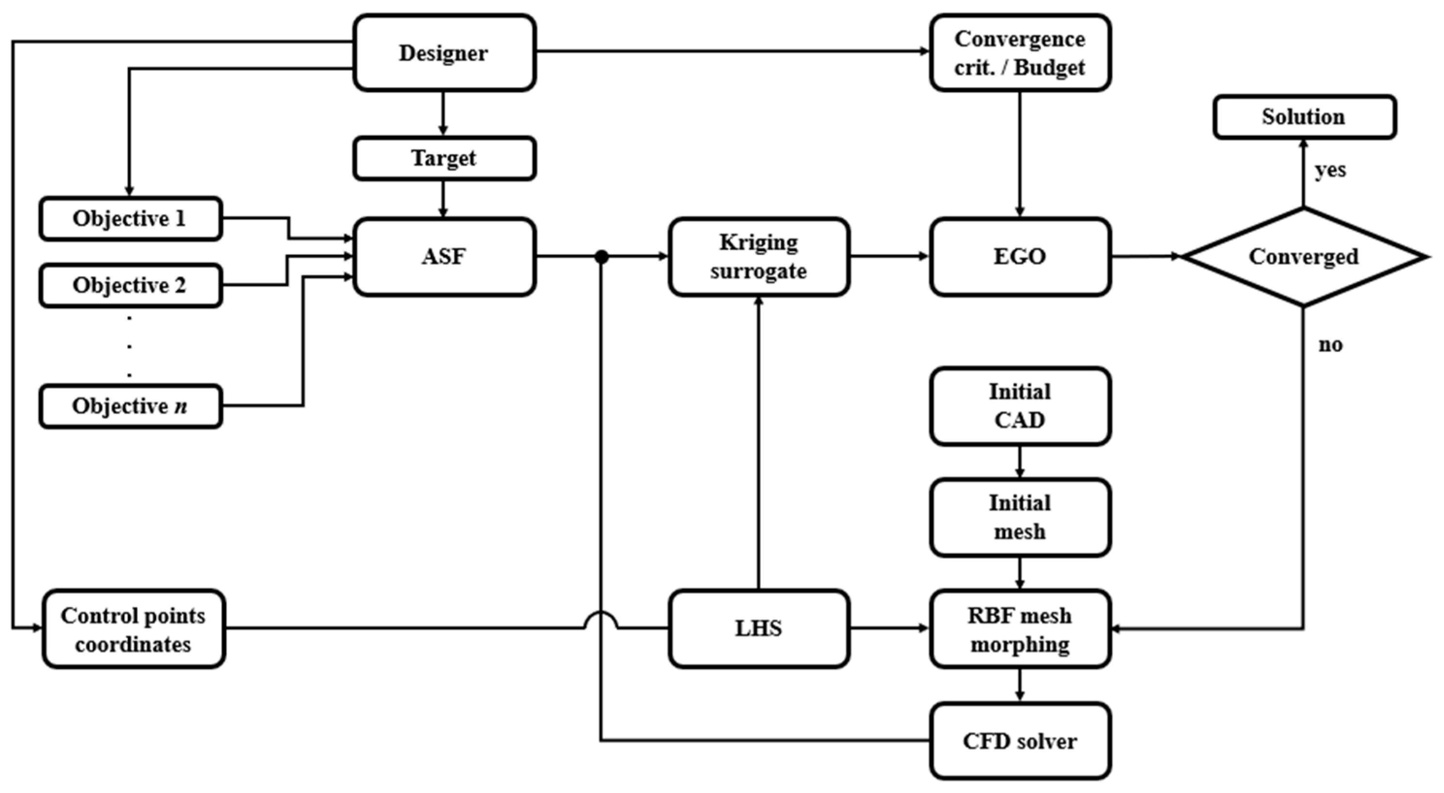
Figure 1. Schematic representation of the optimization framework.
Aerospace 10 00266 g001
Figure 2. Non-convex Pareto front in different methods: (a) weighted sum, (b) reference point.
Aerospace 10 00266 g002
Figure 3. Initial mesh with an indication of flow stations and mesh morpher control points’ locations.
Aerospace 10 00266 g003
Figure 4. Illustration of min θ [ 0 , 2 π ] P t A I P ( θ π 6 , θ + π 6 ) evaluation process at the AIP. The blue segment represents the pressure averaging region.
Aerospace 10 00266 g004
Figure 5. Prediction of normalized longitudinal (U) and circumferential (V) velocity components for various turbulence models in a 180° curved duct with a circular cross-section. Station: (a,b) at 90° bend; (c,d) two diameters downstream of the curved section. Adapted from [37].
Aerospace 10 00266 g005
Figure 6. O-H grid at the duct’s AIP.
Aerospace 10 00266 g006
Figure 7. Results of the duct grid independence study. L = duct centerline length. Numerical values indicate the number of mesh elements.
Aerospace 10 00266 g007
Figure 8. LOO−CV plots for various objective function transformations. Blue lines indicate locations of perfect predictions.
Aerospace 10 00266 g008
Figure 9. Plots of standardized cross-validated residuals for various objective function transformations. Red dashed lines indicate interval of +/− 3 standard deviations.
Aerospace 10 00266 g009
Figure 10. Q−Q plot for various objective function transformations. Blue lines indicate target normal distribution.
Aerospace 10 00266 g010
Figure 11. The effect of FANOVA analysis on model considering 12 variables. Bar height indicates the total effect Sobol’ index value; black color represents the main effect index, and gray color denotes all higher-order interactions.
Aerospace 10 00266 g011
Figure 12. Assessment of deformed mesh quality: (a) mesh orthogonality angle distribution at the duct symmetry plane for a selected solution; (b) histogram of minimum value of mesh elements’ orthogonality angle distribution in all optimization cases. The dashed line indicates the orthogonality angle value for the reference case.
Aerospace 10 00266 g012
Figure 13. Contours of the duct’s symmetry plane for reference and optimized shape.
Aerospace 10 00266 g013
Figure 14. Cumulated minimum value of the ASF (a) and convergence criterion evolution (b) in the course of optimization.
Aerospace 10 00266 g014
Figure 15. Optimization solutions in the objective function space for the three design points. Markers indicate optimization target (target), evaluation of initial geometry (reference), and best obtained solution (best).
Aerospace 10 00266 g015
Figure 16. Details of the distortion coefficient improvements: (a) radially averaged total pressure distribution at AIP. Solid and dashed lines indicate total pressure levels averaged over the AIP and worst 60° sector, respectively; (b) total pressure at AIP normalized by the average dynamic head.
Aerospace 10 00266 g016
Figure 17. Details of the pressure loss coefficient improvements: (a) maps of local pressure loss coefficient; (b) flow streamlines colored by the vertical velocity component at cross−section plane downstream of the AIP.
Aerospace 10 00266 g017
Table 1. Ranges of design variables.
Design VariableRange of Displacement
x 1 , , x 4 ± 100   mm
x 5 ,   x 7 ,   x 8 ± 50   mm
x 6 ± 75   mm
x 9 , , x 12 ± 15   mm
Table 2. Details of operating conditions for considered design points.
Design PointAltitude
(m)
A/C Velocity
(m/s)
Ambient
Pressure
(Pa)
Ambient
Temperature
(K)
Ambient
Density
(kg/m3)
Engine Mass
Flow Rate
(kg/s)
DP1: Nominal cruise30006569,700268.60.9091.5
DP2: Low-altitude climb10046100,129287.51.2131.9
DP3: High-altitude cruise37007164,089264.10.8451.3
Ambient conditions were evaluated with use of the U.S. Standard Atmosphere model [78].
Table 3. Target and nadir points for objectives under selected flight conditions.
Design Point d P D C 60
DP1: Nominal cruisetarget: 10%
nadir: 200%
target: 10%
nadir: 200%
DP2: Low-altitude climbtarget: 5%
nadir: 200%
target: 5%
nadir: 200%
DP3: High-altitude cruisetarget: 5%
nadir: 200%
target: 5%
nadir: 200%
Table 4. ASF transformation functions.
Transforming FunctionDefinition
Natural logarithm ln y
Square root y
Negative inverse square root 1 y
Negative inverse 1 y
Cube root y 3
Table 5. Quantitative optimization results.
ReferenceOptimized Solution
d P D C 60 d P D C 60
Design Point AbsoluteRelativeAbsoluteRelative
DP1: Nominal cruise0.005120.096400.00493−3.71%0.09190−4.67%
DP2: Low-altitude climb0.004590.093690.00443−3.49%0.08943−4.55%
DP3: High-altitude cruise0.004710.096790.00454−3.61%0.09252−4.41%
Disclaimer/Publisher’s Note: The statements, opinions and data contained in all publications are solely those of the individual author(s) and contributor(s) and not of MDPI and/or the editor(s). MDPI and/or the editor(s) disclaim responsibility for any injury to people or property resulting from any ideas, methods, instructions or products referred to in the content.