High-Performance Attitude Control Design of Supersonic Tailless Aircraft: A Cascaded Disturbance Rejection Approach

Abstract

This paper focuses on the triaxial augmentation ability of the active disturbance rejection control (ADRC) technique on the tailless layout with a fully moving wing tip to achieve high control performance for the supersonic tailless aircraft. Firstly, the stability characteristics and controllability of the flying wing layout are analyzed to determine the coupling characteristics of this kind of aircraft. Secondly, an attitude controller is designed based on ADRC theory, and the linear ADRC frequency domain analysis method is introduced to analyze the influence of the bandwidth of linear extended stator on the control system. In addition, the tuning process of the attitude control law is given. Carrier dropping simulations of flight missions under nominal condition, model parameter perturbation, and wind disturbance are conducted. The results show that the designed controller can achieve full-speed domain triaxial augmentation of supersonic flying wing. This work has the potential to significantly boost the engineering acceptability and robustness of supersonic aircraft control design in real-world scenarios. The presented cascaded ADRC approach can significantly improve the performance and robustness of supersonic vehicles.

1. Introduction

1.1. Motivation

In order to ensure the survival rate and operational efficiency of combat aircrafts, stealth performance has become one of the primary technical indicators during the design process of the next generation of fighters [1]. As a result, aircrafts with a small aspect ratio and tailless wing layout take the lead in the potential development trend of the next generation of fighters due to its excellent stealth, low wing load, and high aerodynamic efficiency. In contrast, flying-wing aircrafts often show poor stability under coupling dynamics when performing supersonic flight tasks, which poses a severe threat to the flight safety. Among them, Innovative Control Effector (ICE) aircrafts, a type of highly maneuverable tailless aircrafts, are usually controlled by the interactions between control effectors [2]. Therefore, there is a clear need to improve their controllability, stability, aerodynamics performance and develop the corresponding control laws. In this paper, we demonstrate the controllability of the supersonic ICE aircraft through an airborne launch flight test.

1.2. Related Works

In the work of Zihou He [3], a sample entropy (SampEn) based prescribed performance controller (SPPC) for the longitudinal control of a supersonic tailless aircraft subject to model uncertainty and nonlinearity is proposed. In the work of Mohsen Rostami [4], a multidisciplinary, possibilistic approach is presented to define the sizing of the empennage configuration of a twin-engine propeller-driven aircraft by changing shape parameters while satisfying the design requirements given the tailless aircraft configuration, the flight conditions, and various uncertainties. In the work of Zeyang Zhou [5], to study the influence of spoiler control surface on the radar cross-section (RCS) of a tailless fighter, a calculation method is presented. The deflection angle of the spoiler is controlled by the fixed mode, linear mode, and smooth mode. An aerodynamic design method to improve the high-speed aerodynamic performance of an aircraft with low-aspect-ratio tailless configuration, which can ameliorate the longitudinal moment characteristics of the configuration by designing and collocating the key section airfoils with the constrains of fixed parameters of planform shape and capacity is proposed by Zhongyuan Liu et al [6]. In the study of Bowen Nie et al. [7], they focus on the design of a disturbance rejection controller for a tailless aircraft based on the technique of Nonlinear Dynamic Inversion (NDI), and the tailless aircraft model mounted on a three degree-of-freedom (3-DOF) dynamic rig in the wind tunnel is modeled as a nonlinear affine system subject to mismatched disturbances. An active disturbance rejection controller (ADRC) for suppressing aeroelastic vibrations of a flexible aircraft at the simulation level is proposed by Litao Liu [8]. The recovery landing process was divided into three stages and a reasonable guidance strategy had been designed for them, respectively. Zhao Deng [9] separated the guidance and control issues into an outer guidance loop and an inner control loop. The inner loop (attitude control loop) controlled the UAV to follow the acceleration commands generated by the outer loop (trajectory tracking loop). The inner loop of the longitudinal controller and the lateral controller were designed based on active disturbance rejection control (ADRC), which has strong anti-interference ability. Active Disturbance Rejection Control (ADRC) is utilized by Qi Zhang [10] in the attitude control of a quadrotor aircraft to address the problem of attitude destabilization in flight control caused by parameter uncertainties and external disturbances. Linjie Huang and Hailong Pei [11] propose an improved active disturbance rejection control (IADRC) to solve the problem that the existing robust control method cannot be applied to the SUH with unknown dynamics and disturbances. In addition, in the work of Suiyuan Shen [12], the adaptive radial basis function (RBF) neural network-based active disturbance rejection controller (ADRC) is proposed to enable the unmanned helicopter to fly autonomously in precise paths and to reduce influence of internal and external unknown disturbances on the unmanned helicopters.

1.3. Contribution

This paper focuses on the controllability of supersonic tailless aircrafts. The ADRC frequency-domain analysis and linear extended state controller are combined, making it different from previous research. Throughout an airborne launch flight test, the difficulties and problems of launching separation, powered flight, and unpowered energy management are analyzed. The attitude controller is designed based on the theory of active disturbance rejection control. In addition, the linear active disturbance rejection frequency-domain analysis method is introduced to analyze the influence of the bandwidth of linear extended state controller on the control system, and the tuning flow of the active disturbance rejection attitude control law is given. The flight test is simulated under nominal conditions, model parameter perturbation, and wind disturbance, and the whole mission profile is simulated. The layout of this paper is as follows: in Section 2, the mission characteristics and flight quality (i.e., static stability) are analyzed; in Section 3, the ADRC is first introduced in comparison to the conventional PID control, and then the attitude control laws of the flying-wing aircraft are designed; Section 4 is verification and analysis part through simulation, proving LADRC’s strong dynamic performance robustness.

2. Analysis of Mission Characteristics and Flight Quality

2.1. Overview of Flight Mission

In this test, the ICE aircraft is carried by a carrier and then separated after reaching the predetermined window. After safe separation, it will perform unpowered gliding. Ignition happens when the verifier is at a safety height from the carrier. The flight mission profile is shown in Figure 1. This test is divided into four phases, namely, the launching separation phase, the powered flight phase, the unpowered returning flight phase, and the recovery phase. The definitions are as follows:

(1)

The launching separation phase: It mainly completes the safe separation of the ICE aircraft from the carrier. After safe separation, the ICE aircraft will slide in a stable attitude. When the vertical distance between the carrier and ICE aircraft reaches a safe value, the first phase ends.

(2)

The powered flight phase: The aircraft changes from a downward gliding mode to a climbing mode. Meanwhile, the embedded booster rocket is ignited. In addition, the ICE aircraft will accelerate to a supersonic airspeed. When the booster is burned out, the powered flight phase ends.

(3)

The unpowered gliding phase: The ICE aircraft manages its energy and adjusts its flight path so that it can successfully enter the circle for final parachute landing.

(4)

The recovery phase: The aircraft further dissipates energy and adjusts to an appropriate altitude and attitude to open the parachute for landing in a specific window.

In order to reduce the risks, the flight test is divided into two steps:

S1

The first step is the unpowered delivery test. Firstly, the ICE aircraft is carried by carrier with 0.7 Mach to a height of 11 km, then delivered in a scheduled area. Secondly, the ICE aircraft glides at a constant airspeed without power. Thirdly, it makes energy management after entering the energy dissipation circle. Finally, the ICE aircraft will fly out of the dissipation circle to parachute in the landing windown.

S2

The second step is ICE aircraft supersonic flight control test. Firstly, the carrier carries aircraft to specific height and delivers it. Secondly, the engine is ignited and the aircraft climbs faster after levelling off. Thirdly, the ICE aircraft enters level deceleration flight stage after reaching scheduled height. After decelerating to a subsonic state, the aircraft makes an unpowered return flight. Finally, it flies out of the dissipation circle to parachute in the landing window for recycling after energy management.

2.2. Flight State Point

The design of nominal path and the restrictive conditions are described as follows:

(1)

There is no lateral maneuver requirement in the supersonic stage.

(2)

Limited by the hinge moment of the all-moving tip, the aircraft needs to climb to reach the target airspeed. Moreover, the corresponding deceleration height of horizontal flight is also limited by dynamic pressure.

(3)

In order to take the comprehensive changes of airspeed and atmospheric density into account to facilitate the flight control design, the fixed dynamic pressure is adopted in the gliding flight.

(4)

After the ICE aircraft guides into the energy circle, the landing window should be guaranteed. The restrictive conditions are determined as follows:

Restriction conditions are determined as follows:

• Original conditions: altitude 11 km, Mach number 0.7 Ma;
• Horizontal flight deceleration conditions: altitude 13 km, maximum flight Mach number 1.4 Ma;
• Terminal conditions: altitude 1.2 km, Mach number 0.3 Ma;

The designed nominal trajectory is shown in Figure 2. Select state points around the nominal flight track where dynamic pressure and mass change are sensitive, as shown in

Table 1. Calculation status points in the launching separation stage.

Height (km)	Mach Number
10	0.6    0.7    0.8
11	0.6    0.7    0.8
12	0.6    0.7    0.8

,

Table 2. Calculation status points in powered flight stage.

Height (km)	Mach Number
11	0.6    0.7    0.8    0.9    1.0
12	0.9    1.0    1.1    1.2
13	1.0    1.1    1.2    1.3    1.4    1.5    1.6

and

Table 3. Calculation status points in the recovery stage.

Height (km)	Mach Number
1	0.2    0.3    0.4
3	0.3    0.4    0.5
5	0.3    0.4    0.5    0.6
7	0.4    0.5    0.6    0.7
9	0.6    0.7    0.8
11	0.6    0.7    0.8    0.9
13	0.8    0.9    1.0    1.1    1.2 1.3    1.4    1.5    1.6

.

These state points also serve as the basis for stability and trajectory sensitivity analysis.

2.3. Aerodynamic Layout

The ICE aircraft has a total of four control mechanisms, as shown in Figure 3, including all-moving tip, elevons, and leading edge flaps. Its control distribution is the following:

(a)

The inner and outer ailerons are utilized to control aircraft pitch motion;

(b)

The outer aileron are utilized to control roll motion;

(c)

The all-moving tip is utilized to control yaw motion;

(d)

The accompanying roll moment generated by the all-moving tip can be compensated by the outer aileron motion.

2.4. Flight Quality Analysis

2.4.1. Longitudinal Stability Analysis

The aerodynamic data were acquired by carrying out wind tunnel experiments, which provided high-quality data to ensure the fidelity of the simulation. The center of aerodynamic pressure moves backward with the increase of Mach number, which poses the static stability increases. As shown in Figure 4, the maximum static stability $\frac{d{C}_m}{d{C}_L}$ [13] is about 24% of MAC, which meets the controllability requirements.

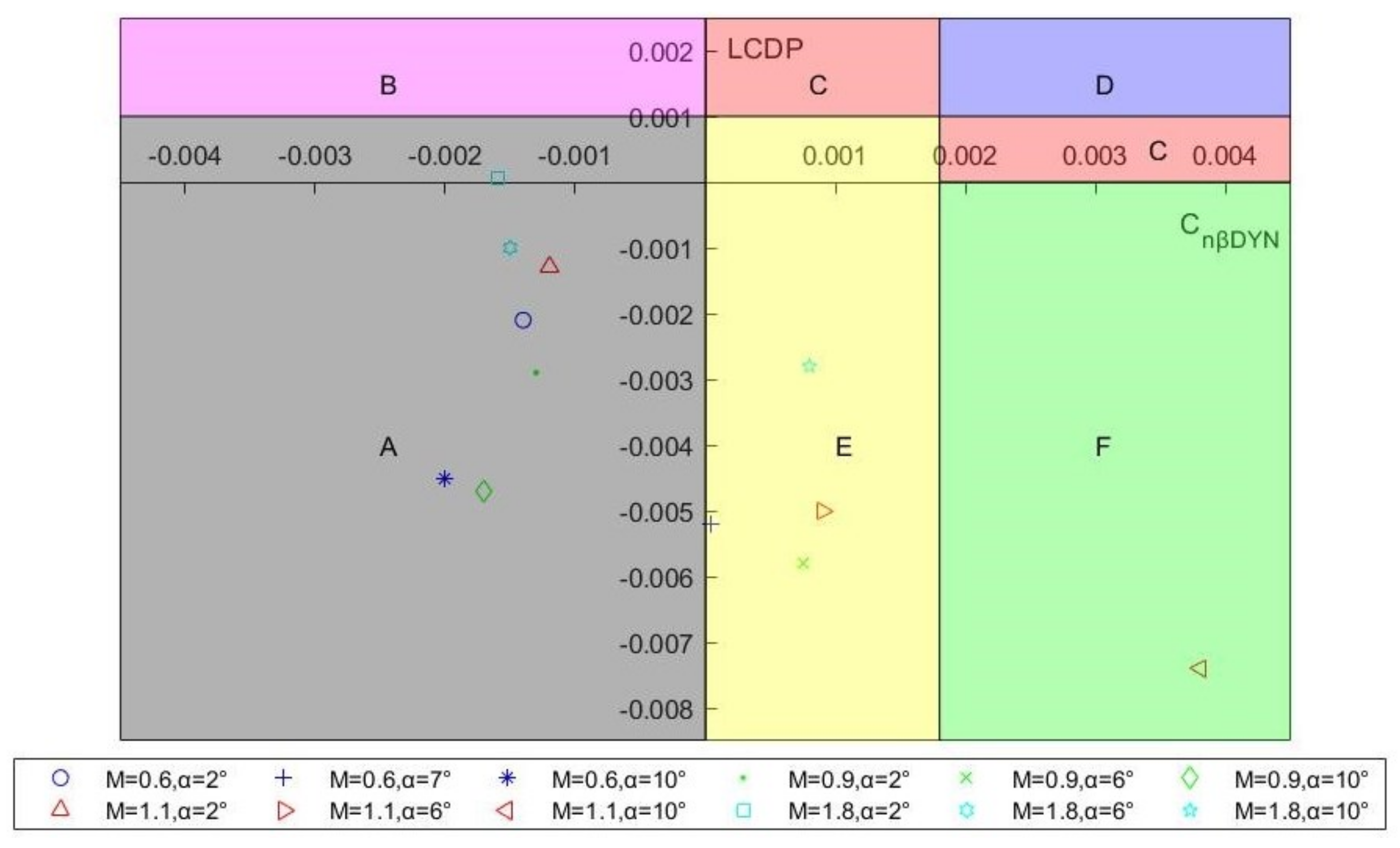
2.4.2. Lateral Stability Analysis

The lateral-directional stability criteria are listed as follows:

• Derivative of directional static stability $C_{n\beta }>0$;
• Derivative of lateral static stability $C_{l\beta }<0$;
• The lateral departure parameter $C_{n\beta ,dyn}>0$;
• Lateral control departure parameter $LCDP>0$;

For directional static stability, the vertical tail, as the main source of lateral force $C_{n\beta }$, is the primary component to provide directional stability $C_{n\beta }$ and yaw damping $C_{nr}$. Therefore, for an ICE aircraft, directional stability $C_{n\beta }$ is less than zero, making it tend to be unstable. In addition, the yaw damping derivatives $C_{nr}$ and roll sensitivity derivatives $C_{lr}$ are much smaller than conventional aircrafts, which makes it more necessary to stabilize the direction.

The lateral departure parameter $C_{n\beta ,dyn}$ is generally used to determine Dutch roll stability, and the calculation formula is shown in Equation (1):

$$\begin{array}{c}\hfill C_{n\beta ,dyn}=C_{n\beta }cos\alpha -\frac{I_z}{I_x}{C}_{l\beta }sin\alpha \end{array}$$

(1)

where, $I_z$ and $I_x$ are the rotational inertia and $\alpha$ is angle of attack.

Accordingly, the Lateral Control Departure Parameters ($LCDP$) can be utilized to predict the directional stability. It represents the directional divergence phenomenon caused by the adverse directional moment exceeding the directional static stability moment, and the formula is shown in Equation (2):

$$\begin{array}{c}\hfill LDCP=C_{n\beta }-\frac{C_{l\beta }{C}_{n{\delta }_a}}{C_{l{\delta }_a}}\end{array}$$

(2)

where, $C_{n{\delta }_a}$ and $C_{l{\delta }_a}$ are control coefficients.

(1)

At a negative angle of attack, $LCDP>0$, directional stability is good; At a positive angle of attack, $LCDP>0$, and it decreases with the increase of angle of attack.

(2)

With the increase of Mach number, it decreases continuously and the directional stability is enhanced.

A more clear Weissman diagram analysis method [13,14] is established through the combination of $C_{n\beta ,dyn}$ and $LCDP$, which can more intuitively and clearly evaluate the aircraft’s lateral directional deviation instability characteristics. According to the range of $C_{n\beta ,dyn}$ and $LCDP$, the Weissman diagram divides the whole diagram into six regions to represent different lateral-course deviation instability states. Figure 5 shows that most of the state points are located in area A, which proves that the lateral characteristics of the aircraft are stable. In supersonic flight at a high angle of attack, some points are scattered in area E, and only one point is in area F. It can be seen from the Weissman criterion diagram that the ICE aircraft has good lateral-directional characteristics and the all-moving tip has good lateral-directional control efficiency in supersonic flight, so the aircraft’s lateral-directional characteristics are stable and controllable.

2.4.3. Conclusion of Flight Quality

From the stability analysis, the results are as follows:

• The longitudinal stability meets the flight quality requirements;
• The center of gravity varies greatly throughout the mission, which poses a challenge to the control law design;
• The relaxation of directional static stability makes the control law high feedback gain requirements, which poses serious risk of robustness.

3. Attitude Control Design

The control difficulties faced by the flight mission are analyzed:

• In the launching separation phase, the strong aerodynamic coupling between the ICE aircraft and the carrier is difficult to accurately analyze through simulation;
• The flow field in the delivery phase has strong aerodynamic interference, which puts forward high requirements on the disturbance rejection ability of the controller;
• Since the booster is buried inside the ICE aircraft, there exist different mass characteristics at the same altitude and Mach number in the flight profile; the designed control law should be robust enough to cope with the unique mass characteristics changes;
• Booster combustion makes the vehicle’s center of gravity move forward. Meanwhile, the subsonic transjump supersonic process makes the aerodynamic focus move back rapidly, resulting in the longitudinal strong static instability rapidly into strong static stability. As a result, the control law needs to have attitude tracking ability with strong robustness and disturbance resistance;
• The thrust line of the booster has position and angle error, and there is a large instantaneous moment at the moment of ignition, which puts forward higher requirements for the anti-disturbance ability of attitude control.

It can be concluded that ICE aircraft is characterized by strong statically unstable, new coupling manipulator, etc. Conventional control methods such as gain scheduling Proportion Integration Differentiation (PID) control have limitations: the PID controller has a poor ability to deal with the situation of ICE aircraft with different static stability characteristics in the same altitude and Mach number status. ADRC is a new practical control technology which combines PID control with modern control theory [15,16,17]. It regards all uncertainties of the system as unknown total disturbances and compensates for them in real time [18,19,20]. Moreover, the design of the control law does not depend on the precise model. ADRC has many advantages such as small computation, high control precision, and good dynamic performance. Therefore, this section will design ICE aircraft attitude control law based on active disturbance rejection control technology.

The principle of the methodology is mainly derived from [17,21]. We first provide a cascaded ADRC attitude control approach, as shown in Figure 6. The control scheme divides the attitude motion into fast-speed inner and low-speed outer loops. For simplicity, the original LADRC is adjusted to the core disturbance rejection attribute: extended state observer (ESO), as shown in Figure 7. Then, frequency domain analysis is introduced to analyze the closed-loop robust performance of the system. Meanwhile, the tuning method of control law gain and observer bandwidth is introduced. Finally, the perturbation simulation of flight test was carried out.

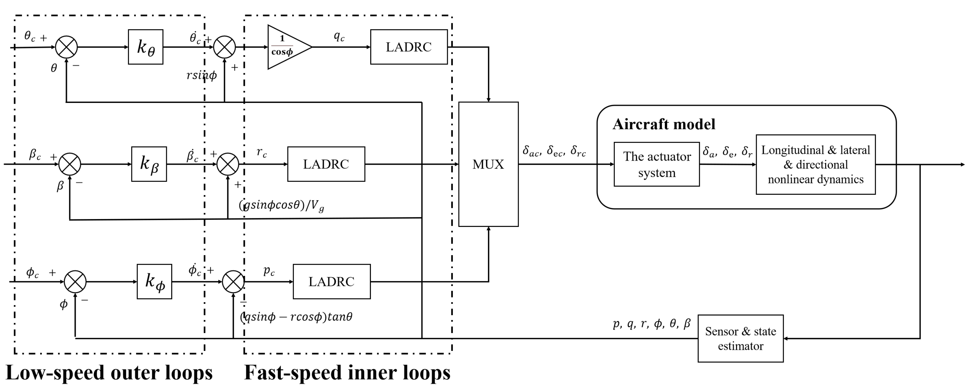
3.1. Cascaded ADRC Attitude Control

3.1.1. Pitch Attitude Control

The pitch angle control adopts proportional control structure, and the angular rate loop adopts LADRC control. As depicted in Figure 6, pitch angular rate command, ${\theta }_c$, can be organized as Equation (3):

$$\begin{array}{c}\hfill \left\{\begin{array}{c}{\dot{\theta }}_c=k_{\theta }\left({\theta }_c-\theta \right)\hfill \\ q_c=\frac{1}{cos\varphi }{\dot{\theta }}_c+rsin\varphi \hfill \end{array}\right.\end{array}$$

(3)

where $\theta$ defines the pitch angle, $\varphi$ defines the roll angle, r is the yaw angular rate, $q_c$ is the pitch angular rate command, and $k_{\theta }$ is the bandwidth of the outer-loop controller.

The kinematic relationship [13] between pitch angle, $\theta$, and its angular rate, q, is shown in Equation (4):

$$\begin{array}{c}\hfill \dot{\theta }=qcos\varphi -rsin\varphi \end{array}$$

(4)

By differentiating both sides of Equation (4), we get:

$$\begin{array}{c}\hfill \ddot{\theta }\approx \dot{q}cos\varphi +q\dot{\varphi }sin\varphi -\dot{r}sin\varphi -r\dot{\varphi }cos\varphi \end{array}$$

(5)

The pitch angular motion around the body $x_b$-axis can be written as the following:

$$\begin{array}{c}\hfill m_a=\dot{q}{I}_y+pr(I_x-I_z)\end{array}$$

(6)

where $m_a$ defines the total pitch moment, $I_y$ is the rotational inertia, and p is the roll angular rate.

From Equation (6), we derive:

$$\begin{array}{c}\hfill \dot{q}=\frac{m_a-pr(I_x-I_z)}{I_y}\end{array}$$

(7)

The general description of the pitch moment coefficient can be written:

$$\begin{array}{c}\hfill C_m=C_{m\alpha 0}+C_{m\alpha }\alpha +{C_m}_{{\delta }_e}{\delta }_e+{C_m}_{q}q\end{array}$$

(8)

where $C_m$ is aero coefficient, $C_{m\alpha 0}$ and $C_{m\alpha }$ are static aero coefficients, ${C_m}_{{\delta }_e}$ is control coefficient, and ${C_m}_q$ is aero coefficient of damping moment.

After substituting Equation (8) in (7) and taking the derivative again:

$$\begin{array}{cc}\hfill \dot{q}& =\frac{(C_{m\alpha 0}+C_{m\alpha }\alpha +{C_m}_{{\delta }_e}{\delta }_e+{C_m}_{q}q)\overline{q}Sc-pr(I_x-I_z)}{I_y}\hfill \\ \hfill & =\frac{(C_{m\alpha 0}+C_{m\alpha }\alpha +C_{mq}q)\overline{q}Sc-pr(I_x-I_z)}{I_y}+\frac{{C_m}_{{}_{{\delta }_e}}\overline{q}Sc}{I_y}{\delta }_e\hfill \\ \hfill & =\frac{(C_{m\alpha 0}+C_{m\alpha }\alpha +C_{mq}q)\overline{q}Sc-pr(I_x-I_z)}{I_y}+{\overline{M}}_{{\delta }_e}{\delta }_e\hfill \end{array}$$

(9)

where ${\overline{M}}_{{\delta }_e}$ is the pitching control efficiency, S is the wing area, c is the reference chord length, and $\overline{q}$ is dynamic pressure. This is then substituted into the above formula, and the following equation can be obtained:

$$\begin{array}{cc}\hfill \ddot{\theta }& \approx -\dot{r}sin\varphi -r\dot{\varphi }cos\varphi +q\dot{\varphi }sin\varphi \hfill \\ \hfill & +\left(\frac{(C_{m\alpha 0}+C_{m\alpha }\alpha +C_{mq}q)\overline{q}Sc-pr(I_x-I_z)}{I_y}+{\overline{M}}_{{\delta }_e}{\delta }_e\right)cos\varphi \hfill \\ \hfill & =-\dot{r}sin\varphi -r\dot{\varphi }cos\varphi +q\dot{\varphi }sin\varphi \hfill \\ \hfill & +\frac{(C_{m\alpha 0}+{C_m}_{\alpha }\alpha +{C_m}_{q}q)\overline{q}Sc-pr(I_x-I_z)}{I_y}cos\varphi +{\overline{M}}_{{\delta }_e}cos\varphi {\delta }_e\hfill \end{array}$$

(10)

With the substitution of $b_q={\overline{M}}_{{\delta }_e}cos\varphi$ and $y=\dot{\theta }$, the above equation can be written:

$$\begin{array}{cc}\hfill \dot{y}& =-\dot{r}sin\varphi -r\dot{\varphi }cos\varphi +q\dot{\varphi }sin\varphi \hfill \\ \hfill & +\frac{(C_{m\alpha 0}+C_{m\alpha }\alpha +{C_m}_{q}q)\overline{q}Sc-pr(I_x-I_z)}{I_y}cos\varphi +b_q{\delta }_e\hfill \end{array}$$

(11)

Define:

$$\begin{array}{c}\hfill \left\{\begin{array}{c}{x}_1=y\hfill \\ x_2=-\dot{r}sin\varphi -r\dot{\varphi }cos\varphi +q\dot{\varphi }sin\varphi \hfill \\ +\frac{(C_{m\alpha 0}+C_{m\alpha }\alpha +C_{mq}q)\overline{q}Sc-pr(I_x-I_z)}{I_y}cos\varphi \hfill \end{array}\right.\end{array}$$

(12)

Then, Equation (12) can be described in terms of the state space form:

$$\begin{array}{c}\hfill \left\{\begin{array}{c}{\dot{x}}_1=x_2+b_q{\delta }_e\hfill \\ {\dot{x}}_2=f_q\hfill \\ y=x_1\hfill \end{array}\right.\end{array}$$

(13)

where $f_q$ is assumed to be a lumped disturbance which contains unmodeled dynamic and dynamic coupling terms. Now, the state of Equation (13) $x_2\approx z_{q2}$ can be estimated through ESO.

Correspondingly, the control law can be written:

$$\begin{array}{c}\hfill {\delta }_e=\frac{{\delta }_0-z_{q2}}{b_q}\end{array}$$

(14)

Then, the original system can be transformed:

$$\begin{array}{c}\hfill \dot{y}\approx {\delta }_0\end{array}$$

(15)

The original equation is equivalent to a first-order integral, and the static difference of the output can be eliminated by proportional control. Considering that the final controlled quantity is the pitch angle rate of the aircraft, the form of virtual control input is taken as the most commonly used proportional control form in engineering:

$$\begin{array}{c}\hfill {\delta }_0=\frac{k_q(q_c-q)}{b_q}\end{array}$$

(16)

In summary, the complete control law is:

$$\begin{array}{c}\hfill {\delta }_e=\frac{k_q(q_c-q)-z_{q2}}{b_q}\end{array}$$

(17)

where, $k_q$ is the pitch angle rate control bandwidth, and $b_q$ is the pitch control efficiency varying with dynamic pressure. Here, $\dot{\theta }\approx q$, and the corresponding ESO is the following:

$$\begin{array}{c}\hfill \left\{\begin{array}{c}{\dot{z}}_{q1}=z_{q2}+{\beta }_{q1}(q-z_{q1})+b_q{\delta }_e\hfill \\ {\dot{z}}_{q2}={\beta }_{q2}(q-z_{q1})\hfill \end{array}\right.\end{array}$$

(18)

where ${\beta }_{q1}$ and ${\beta }_{q2}$ is the ESO gain of pitch second order and $z_{q1}$ is the estimation of pitch angle rate q.

3.1.2. Roll Attitude Control

Roll angle control adopts proportional control structure, and roll angular roto loop adopts LADRC control. The control structure is shown in Figure 6. Similar to pitch channel, the roll channel control law is the following:

$$\begin{array}{c}\hfill {\delta }_a=\frac{k_p(p_c-p)-z_{p2}}{b_p}\end{array}$$

(19)

where $z_{p2}$ is ESO’s estimation of the total disturbance, $k_p$ is roll angular rate control bandwidth, and $b_p$ is roll control efficiency varying with dynamic pressure.

The corresponding ESO is the following:

$$\begin{array}{c}\hfill \left\{\begin{array}{c}{\dot{z}}_{p1}=z_{p2}+{\beta }_{p1}(p-z_{p1})+b_p{\delta }_a\hfill \\ {\dot{z}}_{p2}={\beta }_{p2}(p-z_{p1})\hfill \end{array}\right.\end{array}$$

(20)

where ${\beta }_{p1}$ and ${\beta }_{p2}$ are the ESO gain of roll second order and $z_{p1}$ is the estimation of roll angle rate p.

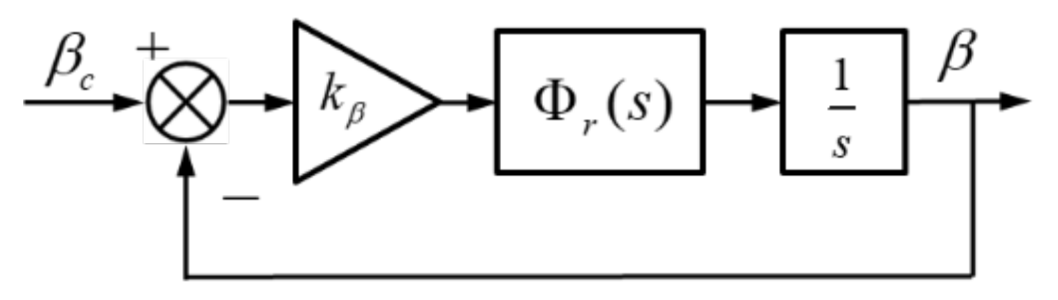
3.1.3. Sideslip Angle Control

Sideslip angle control adopts proportional control structure, and LADRC control is used for yaw angular rate loop. The control structure is as follows in Figure 6. Sideslip angle control law is designed as the following:

$$\begin{array}{c}\hfill \left\{\begin{array}{c}{\dot{\beta }}_c=k_{\beta }\left({\beta }_c-\beta \right)\hfill \\ r_c={\dot{\beta }}_c+\left(gsin\varphi cos\theta \right)/\phantom{\left(gsin\varphi cos\theta \right)V_g}{V}_g\hfill \end{array}\right.\end{array}$$

(21)

Similar to roll channel Equation (19), the yaw channel controller can be stated:

$$\begin{array}{c}\hfill {\delta }_r=\frac{k_r(r_c-r)-z_{r2}}{b_r}\end{array}$$

(22)

where $z_{r2}$ is the estimation of total disturbance by ESO, $k_r$ is the yaw angular rate control bandwidth, and $b_r$ is the yaw control efficiency varying with dynamic pressure.

The corresponding ESO is the following:

$$\begin{array}{c}\hfill \left\{\begin{array}{c}{\dot{z}}_{r1}=z_{r2}+{\beta }_{r1}(r-z_{r1})+b_r{\delta }_r\hfill \\ {\dot{z}}_{r2}={\beta }_{r2}(r-z_{r1})\hfill \end{array}\right.\end{array}$$

(23)

where ${\beta }_{r1}$ and ${\beta }_{r2}$ are ESO gain of yaw second order, and $z_{r1}$ and $z_{r2}$ are the estimation of yaw angle rate r.

3.1.4. The Design of Soft and Hard Cross-Connection

Increasing the soft and hard cross-connection is helpful to reduce the coupling effect between the three channels. Coupling exists in the lateral-to-vertical, lateral-to-directional, and directional-to-vertical relationships.

The design principle of hard cross-connection is to assign the virtual total efficiency to ailerons and AMT according, and its control law is:

$$\begin{array}{c}\hfill {\delta }_a=k_{dr2da}{\delta }_r\end{array}$$

(24)

$$\begin{array}{c}\hfill {\delta }_r=k_{da2dr}{\delta }_a\end{array}$$

(25)

where $k_{dr2da}$ and $k_{d\mathrm{a}2dr}$ are the hard cross-connection gain.

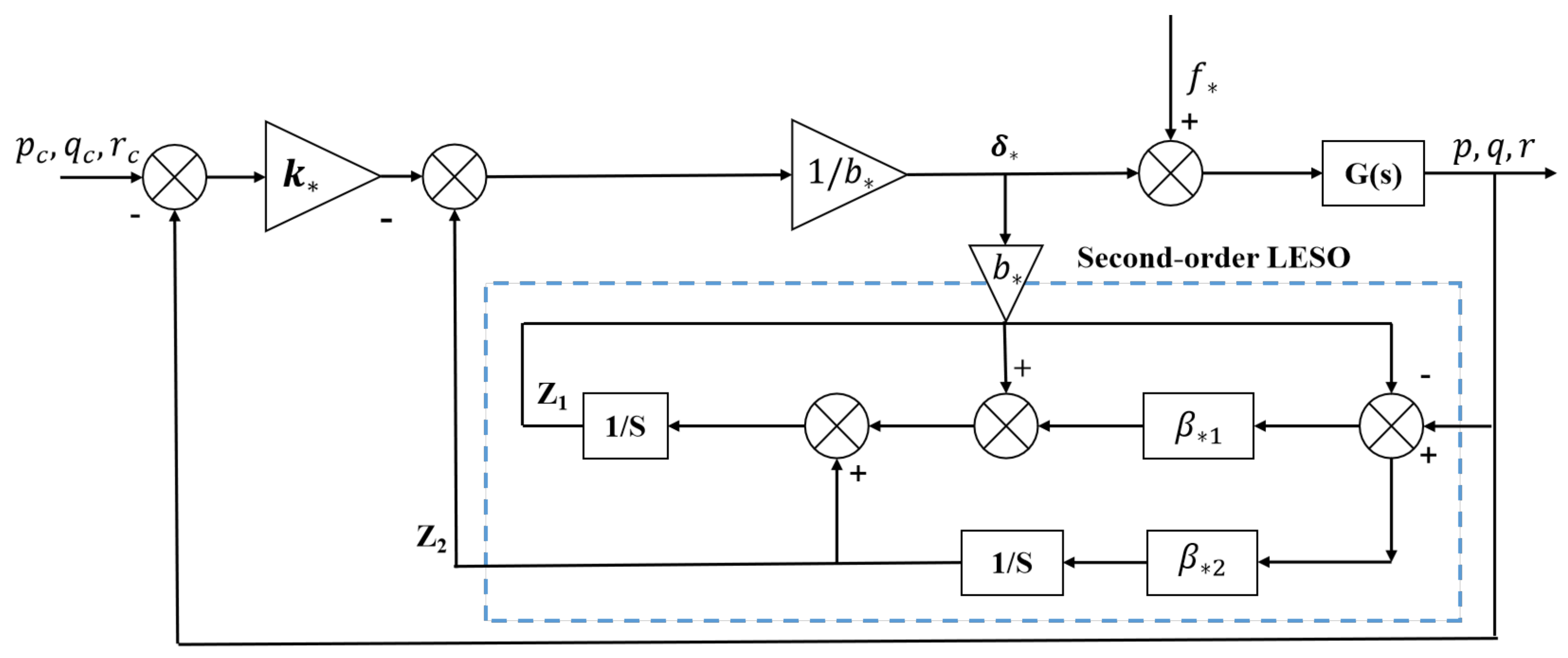
3.2. Linear Extended State Observer

3.2.1. Proof of LESO Convergence

The LESO observer is shown as follows:

$$\begin{array}{c}\hfill \left\{\begin{array}{c}{e}_r=\widehat{r}-r\hfill \\ \dot{\widehat{r}}={\widehat{f}}_r-{\beta }_{r1}{e}_r+b_r{\delta }_r\hfill \\ {\dot{\widehat{f}}}_r=-{\beta }_{r2}{e}_r\hfill \end{array}\right.\end{array}$$

(26)

where ${\beta }_{r1}$ and ${\beta }_{r2}$ are 2n-leso parameters; $\widehat{r}$ and ${\widehat{f}}_r$ are estimates of r and $f_r$ respectively; and $b_r$ is the yaw control efficiency.

Setting ${\dot{f}}_r=h_r$, and combining with Equation (26), we get:

$$\begin{array}{c}\hfill \left\{\begin{array}{c}\dot{r}-\dot{\widehat{r}}=f_r-{\widehat{f}}_r-{\beta }_{r1}\left(r-\widehat{r}\right)\hfill \\ f_r-{\dot{\widehat{f}}}_r=h_r-{\beta }_{r2}\left(r-\widehat{r}\right)\hfill \end{array}\right.\end{array}$$

(27)

Rewriting this as a matrix:

$$\begin{array}{c}\hfill {\dot{X}}_r-{\dot{\widehat{X}}}_r=\left(A-L\right)\left(X_r-{\widehat{X}}_r\right)+B_2{h}_r\end{array}$$

(28)

where $X_r={[r,f_r]}^T$, ${\widehat{X}}_r={[\widehat{r},{\widehat{f}}_r]}^T$; Matrix A, L, and $B_2$ are expressed as follows:

$$\begin{array}{c}\hfill A=\left[\begin{array}{cc}0& 1\\ 0& 0\end{array}\right],L=\left[\begin{array}{cc}{\beta }_{r1}& 0\\ {\beta }_{r2}& 0\end{array}\right],B_2={\left[\begin{array}{cc}0& 1\end{array}\right]}^{\mathrm{T}}\end{array}$$

(29)

when the matrix $A-L$ is Hurwitz, the estimation error $X_r-{\widehat{X}}_r$ tends to zero. Then, the roots of the characteristic equation should have negative real parts. The characteristic equation is expressed as follows:

$$\begin{array}{c}\hfill \left|\left.\lambda {\mathrm{I}}_2-(A-L)\right|\right.={\lambda }^2+{\beta }_{r1}\lambda +{\beta }_{r2}=\prod _{i=2}^2\left(\lambda +{\lambda }_i\right)\end{array}$$

(30)

where ${\lambda }_i$ is a constant.

Theorem 1.

It is assumed that the total disturbance $f_r$ and its derivatives $h_r$ are bounded, that is $\left|f_r\right|\le \xi$ and $\left|h_r\right|\le \overline{\xi }$, where ξ and $\overline{\xi }$ are positive real numbers. When ${\lambda }_i$ are positive numbers, there is always LESO so that the estimation error is bounded.

According to Theorem 1, the convergence conditions of 1, 2 N-leso are: all ${\lambda }_i$ are positive numbers. When ${\beta }_{r1}=2{\omega }_0$ and ${\beta }_{r2}={\omega }_0^2$, Equation (30) can be rewritten as:

$$\begin{array}{c}\hfill {\lambda }^2+{\beta }_{r1}\lambda +{\beta }_{r2}={\left(\lambda +{\omega }_0\right)}^2\end{array}$$

(31)

where, ${\omega }_0$ is also known as the LESO bandwidth and ${\omega }_0>0$.

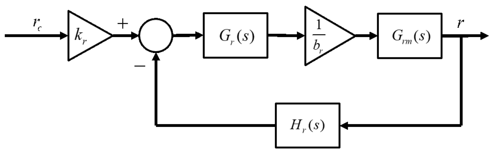
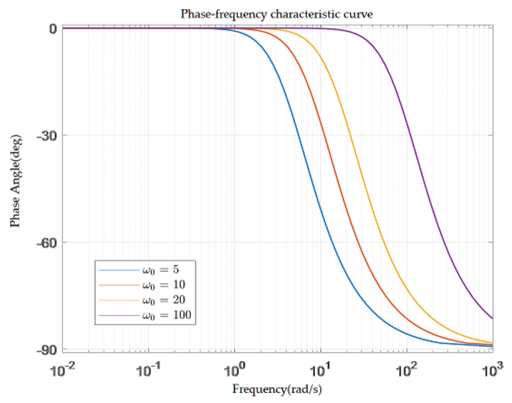
3.2.2. The Setting of LESO Bandwidth

The effect of LESO bandwidth ${\omega }_0$ on system performance is analyzed [22,23]. Since LESO is a nonlinear function, the observer performance can be analyzed in the frequency domain. Taking sideslip angle channel as an example, the control law can be simplified:

$$\begin{array}{c}\hfill \left\{\begin{array}{c}{r}_c=k_{\beta }\left({\beta }_c-\beta \right)\hfill \\ {\delta }_r=\frac{k_r\left(r_c-r\right)-f_r}{b_r}\hfill \end{array}\right.\end{array}$$

(32)

Firstly, the loop-opening transfer function is established. According to Equation (32), 2N-LESO can be rewritten as:

$$\begin{array}{c}\hfill \left\{\begin{array}{c}\widehat{r}s={\widehat{f}}_r-{\beta }_{r1}\left(\widehat{r}-r\right)+b_r{\delta }_r\hfill \\ {\widehat{f}}_{r}s=-{\beta }_{r2}(\widehat{r}-r)\hfill \end{array}\right.\end{array}$$

(33)

where s is the domain of the transfer function.

Its corresponding transfer function is the following:

$$\begin{array}{c}\hfill \widehat{r}=\frac{{\beta }_{r1}s+{\beta }_{r2}}{s^2+{\beta }_{r1}s+{\beta }_{r2}}r+\frac{b_{r}s}{s^2+{\beta }_{r1}s+{\beta }_{r2}}{\delta }_r\end{array}$$

(34)

$$\begin{array}{c}\hfill {\widehat{f}}_r=\frac{{\beta }_{r2}s}{s^2+{\beta }_{r1}s+{\beta }_{r2}}r-\frac{{\beta }_{r2}{b}_r}{s^2+{\beta }_{r1}s+{\beta }_{r2}}{\delta }_r\end{array}$$

(35)

Substitute Equation (35) into Equation (32) to obtain:

$$\begin{array}{c}\hfill {\delta }_r=\frac{1}{b_r}\frac{s^2+{\beta }_{r1}s+{\beta }_{r2}}{s^2+{\beta }_{r1}s}\left[k_r{r}_c-\frac{k_r{s}^2+\left(k_r{\beta }_{r1}+{\beta }_{r2}\right)s+k_r{\beta }_{r2}}{s^2+{\beta }_{r1}s+{\beta }_{r2}}r\right]\end{array}$$

(36)

Assuming that the effector is ideal, ${\delta }_{rc}={\delta }_r$; the equivalent form of yaw angular rate control is shown in Figure 8,

Where

$$\begin{array}{cc}\hfill & G_r\left(s\right)=\frac{s^2+{\beta }_{r1}s+{\beta }_{r2}}{s^2+{\beta }_{r1}s}\hfill \end{array}$$

(37)

$$\begin{array}{cc}\hfill & H_r\left(s\right)=\frac{k_r{s}^2+(k_r{\beta }_{r1}+{\beta }_{r2})s+k_r{\beta }_{r2}}{s^2+{\beta }_{r1}s+{\beta }_{r2}}\hfill \end{array}$$

(38)

where $G_{rm}\left(s\right)$ is the transfer function from ${\delta }_r$ to r. Combining Equations (37) and (38), the closed-loop transfer function of the system can be obtained as follows:

$$\begin{array}{c}\hfill {\Phi }_r\left(s\right)=\frac{k_r{G}_r\left(s\right)G_{rm}\left(s\right)}{H_r\left(s\right)G_r\left(s\right)G_{rm}\left(s\right)+b_r}\end{array}$$

(39)

The structure of the yaw angular rate loop control structure is shown in Figure 9.

According to Figure 9, the open-loop transfer function of sideslip angle control system can be obtained:

$$\begin{array}{c}\hfill G_{\beta }\left(s\right)=k_{\beta }{\Phi }_r\left(s\right)\frac{1}{s}\end{array}$$

(40)

According to the open-loop transfer function of sideslip angle and yaw angular rate loop, the state points in Table 1 were selected to analyze the influence of LESO bandwidth value. Taking the state point of 11 km and 0.7 Ma to conduct ESO bandwidth sensitivity analysis, and settings ${\beta }_{r1}=2{\omega }_0$ and ${\beta }_{r2}={\omega }_0^2$, $k_{\beta }=1$ and $k_r=4$, the Bode diagram can be drawn when LESO bandwidth values ${\omega }_0$ are 5, 10, 20, and 30, respectively:

It can be seen from Figure 10 and Figure 11 that, the larger ESO bandwidth ${\omega }_0$, the larger the open-loop cutoff frequency at the effector, thus, reducing the phase angle margin. Figure 11 shows that the response performance of sideslip angle is less affected by bandwidth.

Secondly, the observer bandwidth is also limited by the sensor measurement bandwidth. The transfer function of sensor measurement noise $n_r$ is the following:

$$\begin{array}{c}\hfill \frac{\widehat{r}}{n_r}=\frac{{\beta }_{r1}s+{\beta }_{r2}}{s^2+{\beta }_{r1}s+{\beta }_{r2}}\end{array}$$

(41)

When the observer bandwidth ${\omega }_0$ value is 5, 10, 20, and 100 [21], its amplitude–frequency characteristic curve is shown in Figure 12. Therefore, the larger the bandwidth value ${\omega }_0$, the larger the high-frequency gain, and the observer is more sensitive to measurement noise. The phase frequency characteristic curve is shown in Figure 13. The larger the bandwidth value ${\omega }_0$, the larger the amplitude margin of the phase angle in the high frequency band, and the worse the observer’s suppression of the measured noise. In addition, the value of ${\omega }_0$ is also limited by the calculation frequency of the autopilot, which will cause the jitter of the observed value when it increases to a certain extent.

In practical application, the value of ${\omega }_0$ should be within the acceptable range of noise influence, and the larger value should be taken without causing the jitter of the observed value. Verification from a large number of semi-physical experiments shows that when the calculated step size of the control law is 5 ms, the value of ${\omega }_0$ will be in the range of 10–30.

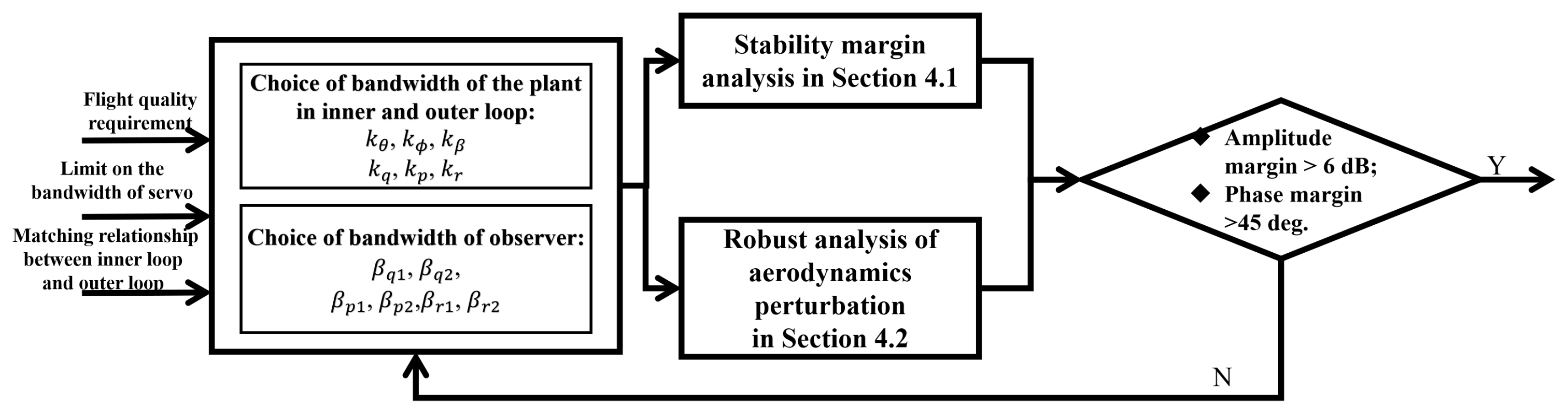
3.2.3. Control Law Tuning Rule

In practical engineering, LESO bandwidth selection is limited by sensor noise and control law cutoff frequency, so it can not be infinite [19,22]. If the ESO estimation error convergence is not fast enough, such that the damping or overshoot of closed-loop performance does not meet the requirements of the index, the controller and ESO gains should be adjusted again. Meanwhile, the control law gain should be further adjusted by fully combining the time domain response and frequency domain response. The selection of bandwidth should consider the matching relationship between the internal and external loop, the bandwidth of the effector, the flight quality requirements of the aircraft, the control ability of the control mechanism, the stability margin of the controller, etc. According to the time scale separation criterion, it is required that the bandwidth of the inner loop is large enough in comparison with the outer loop, and the bandwidth of the effector is large enough in comparison with the inner loop.

The gains setting rule of the cascaded ADRC attitude control is shown in Figure 14, and the specific steps are as follows:

Step 1:

According to the timing separation principle [14], select $k_q$ as 1/5–1/3 of the effector bandwidth. Select $k_{\theta }$ as 1/5 to 1/3 of $k_q$;

Step 2:

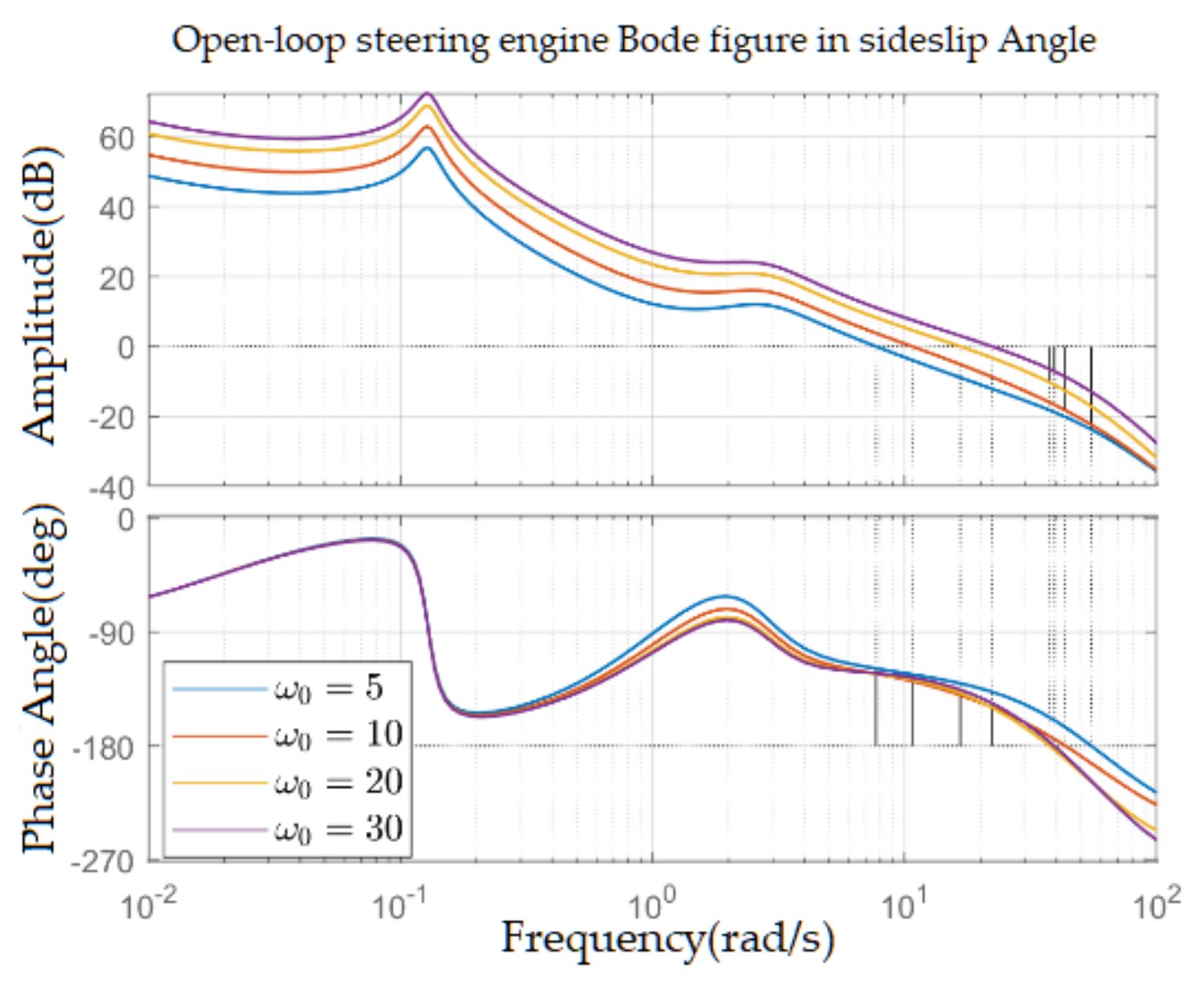
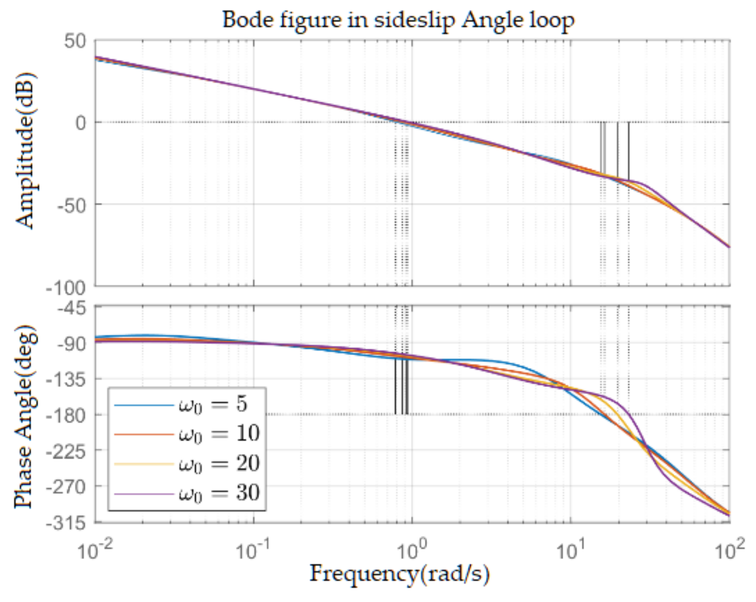
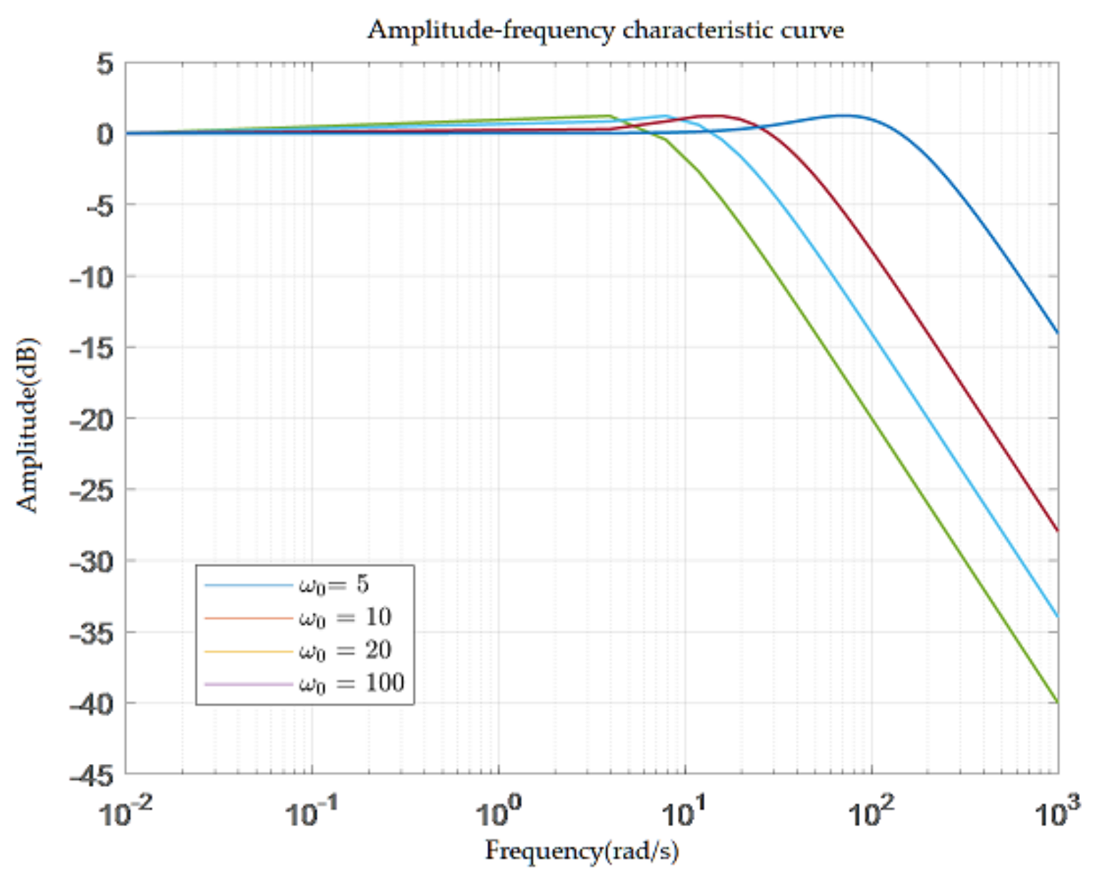
LESO bandwidth should be selected according to the cutoff frequency of the control loop. The selection range of ${\omega }_0$ is generally between 5 and 20, and the selected bandwidth should not cause the ESO oscillation.

Step 3:

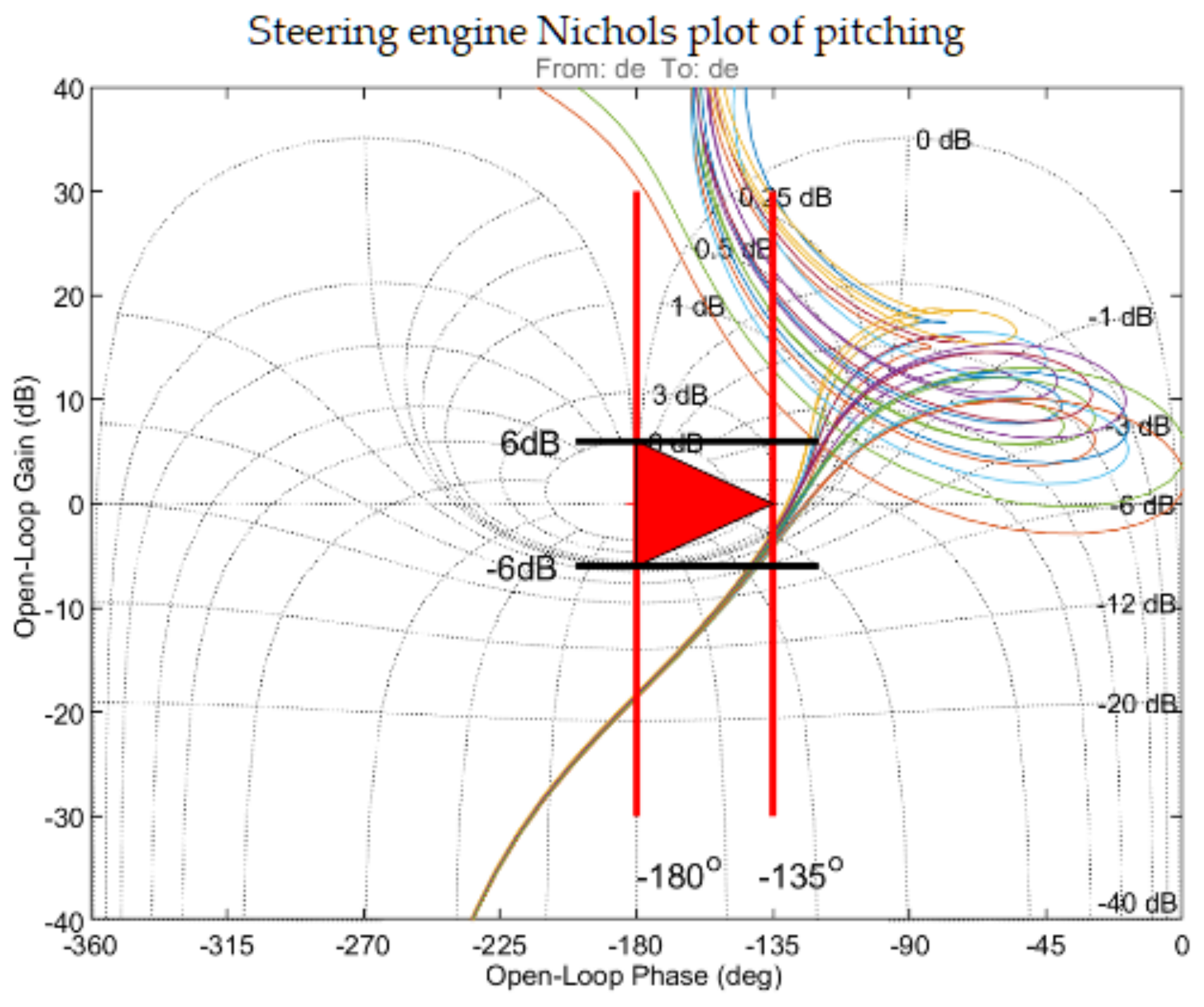
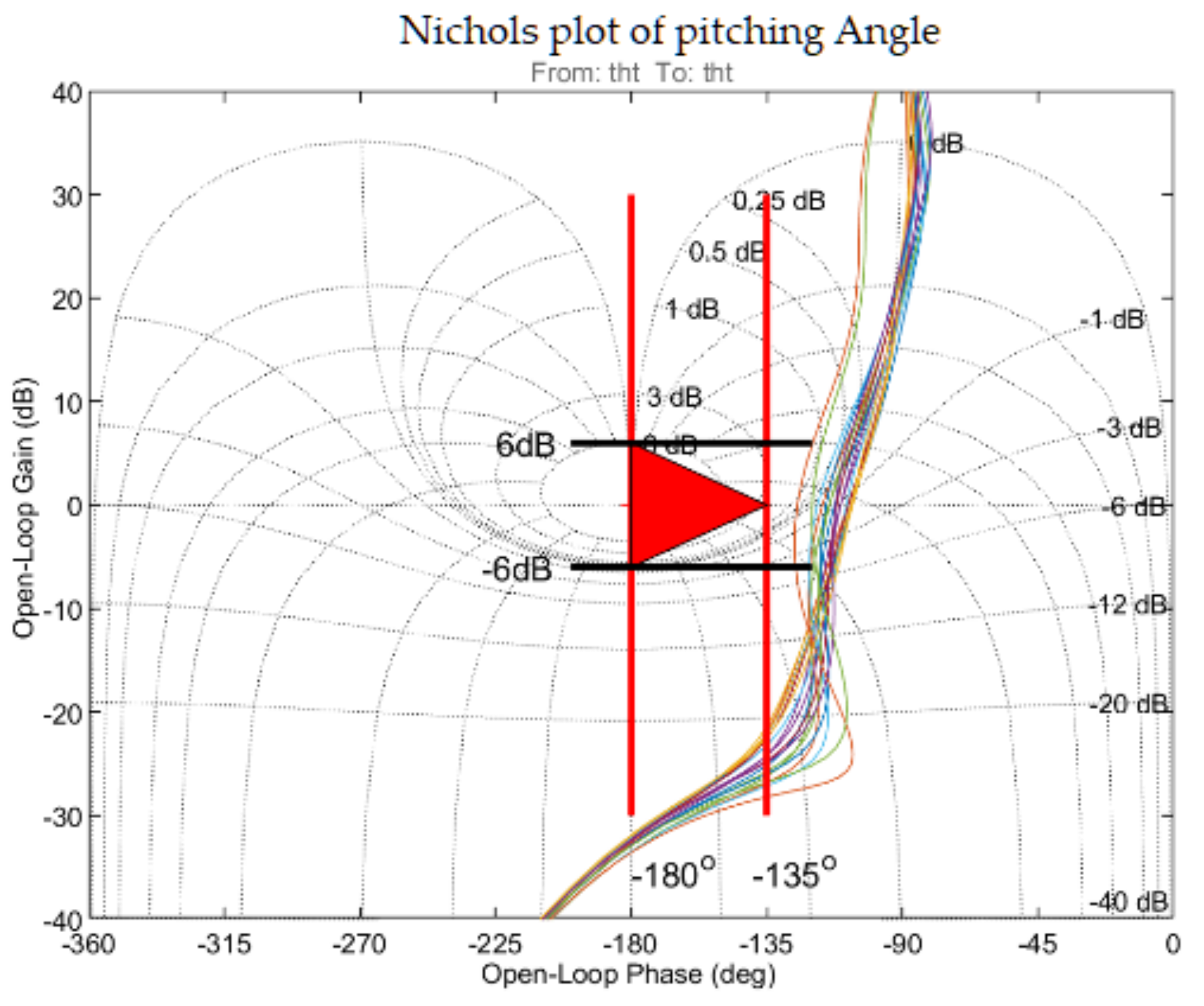
The stable index of amplitude margin and phase angle margin is used to judge whether the controller meets the frequency requirements, and the time-domain response is used to judge whether the system meets the dynamic performance requirements. If it meets the index requirements, the setting ends; otherwise, the next step is carried out.

Step 4:

Adjust the control law gain, $k_{\theta }$, by Nichols diagram or time-domain response curve and return to Step 3.

4. Flight Test Analysis and Verification

4.1. Inner Loop Verification

Taking the longitudinal channel as an example, the status points in Table 1, Table 2 and Table 3 were selected to design the frequency domain of the inner loop. Meanwhile, the sensor data transmission delay was set as 0.0375 ms, and the elevator was modeled as a second-order dynamic system with the bandwidth at 50 rad/s. A nominal verification test was conducted to obtain the bode diagram of open loop at the pitching and elevator, respectively, as shown in Figure 15 and Figure 16. The nominal design satisfies the phase and amplitude margin above 45 deg and 6 dB. In engineering design, the dynamic performance robustness of closed-loop control system can be measured by the phase margin: the smaller the change of phase margin and corresponding intercept frequency, the stronger the dynamic performance robustness of closed-loop system. It can be seen from Figure 15 and Figure 16 that the cutoff frequency is consistent in 55 perturbation states, which indicates that the dynamic performance of the system under the LADRC framework is very robust. It can efficiently deal with flight control problems in a width velocity domain, especially the large variation range of static stability margin with rocket fuel consumption. Step response curves of the small disturbance model corresponding to these 55 perturbation states are shown in Figure 17. It can be seen that the dynamic quality of each state is not only excellent, but also that the step dynamic of all perturbation states are basically the same, which reflects LADRC’s strong dynamic robustness.

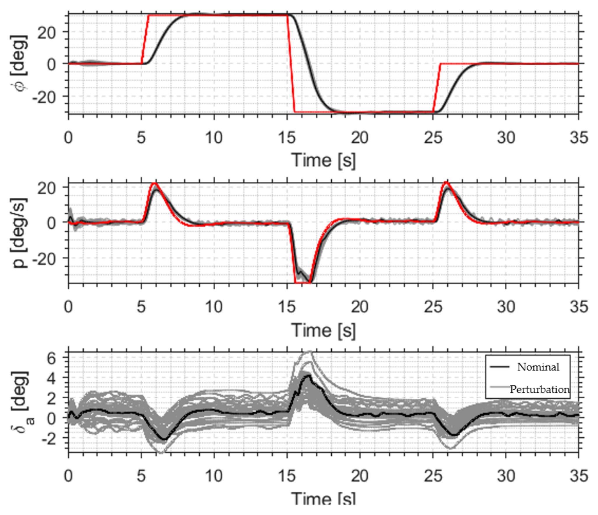
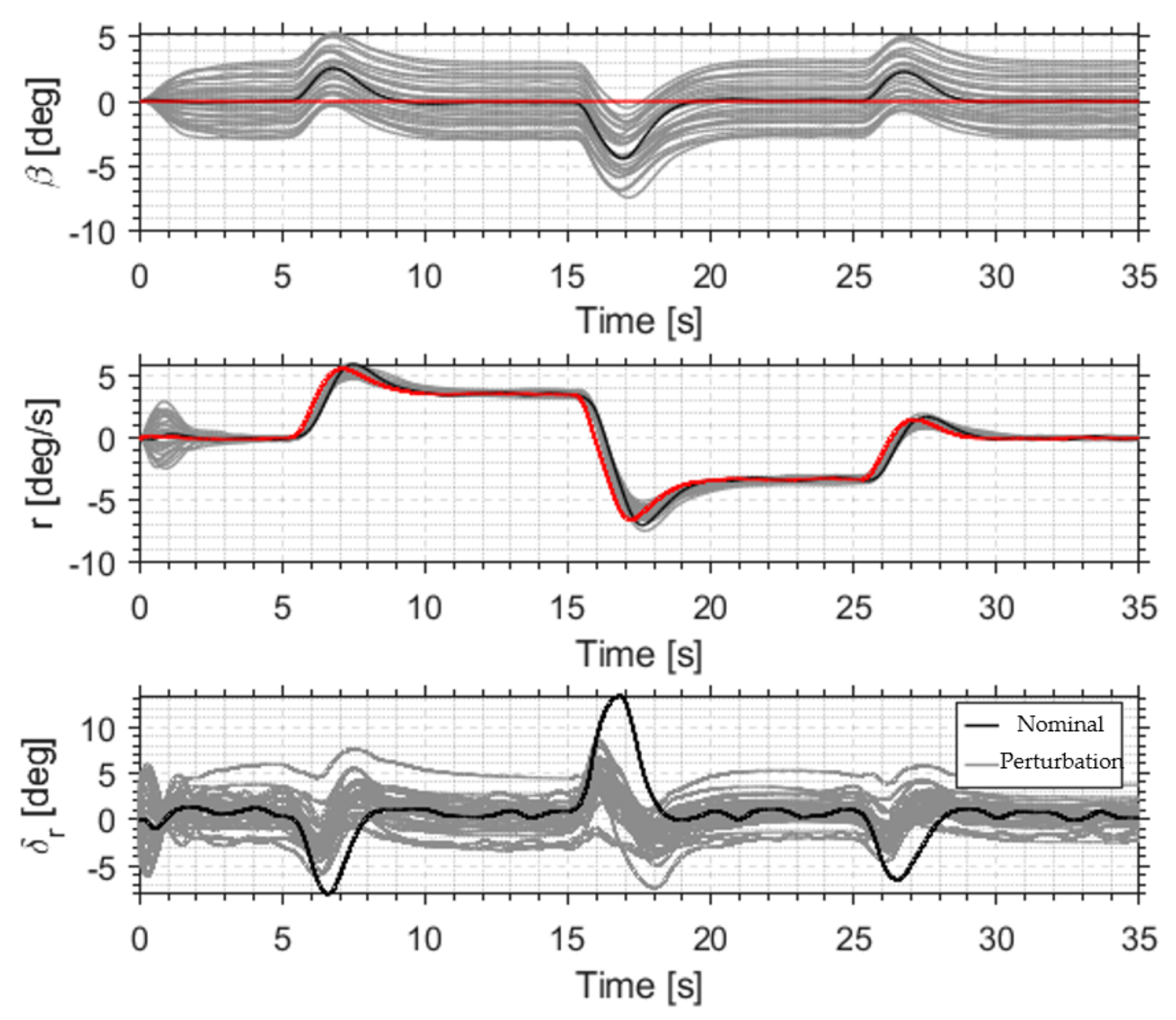
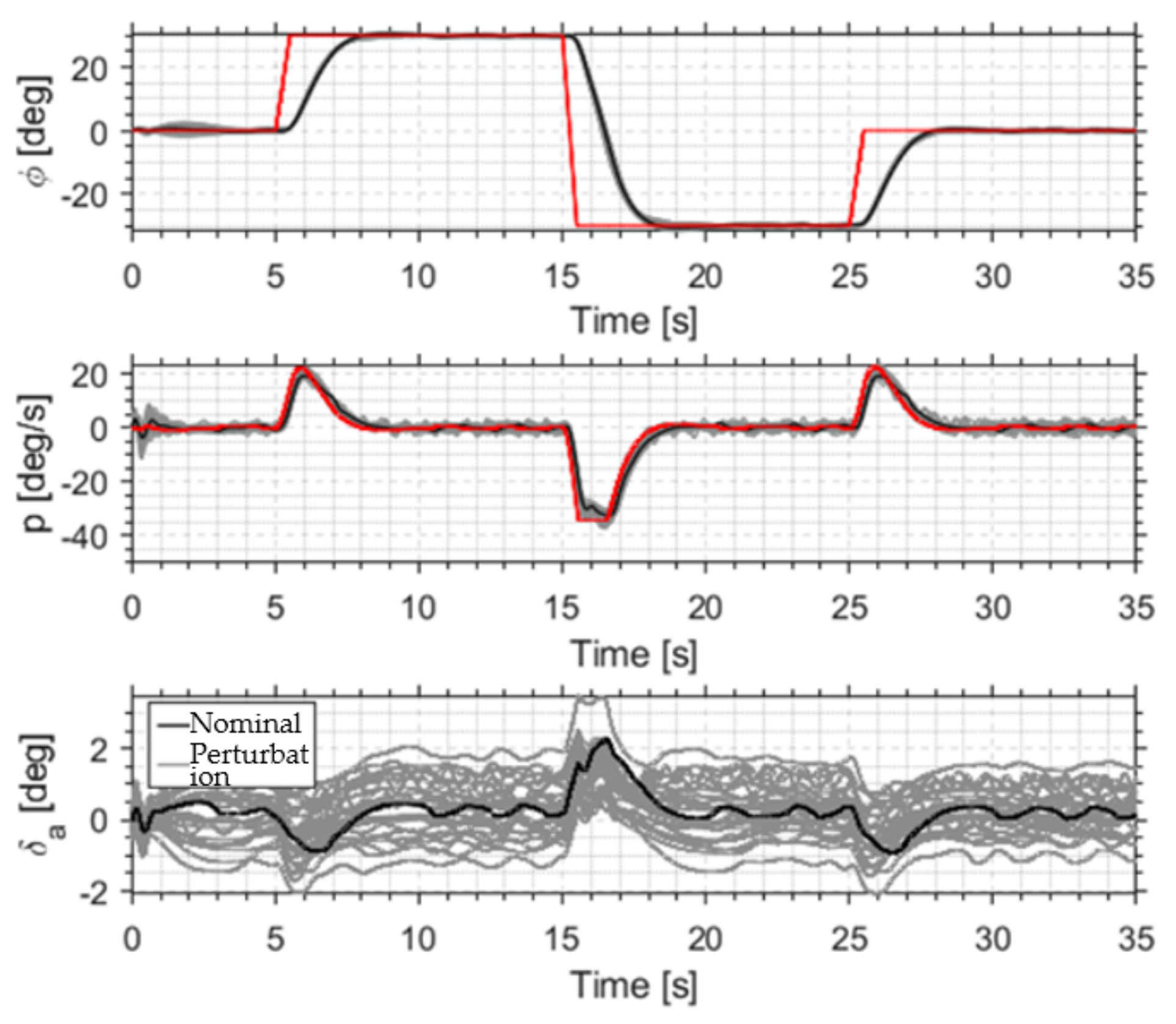
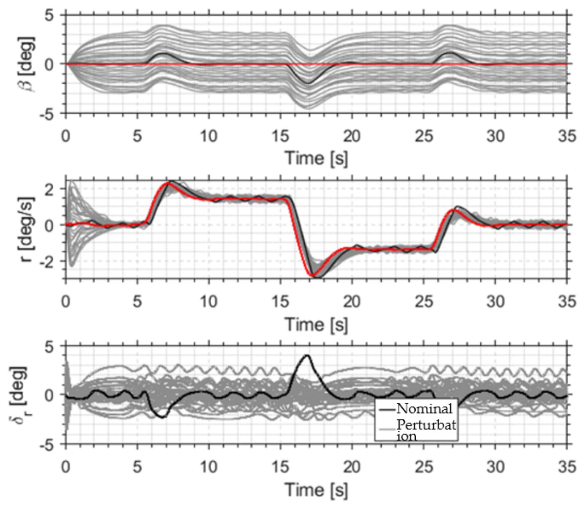
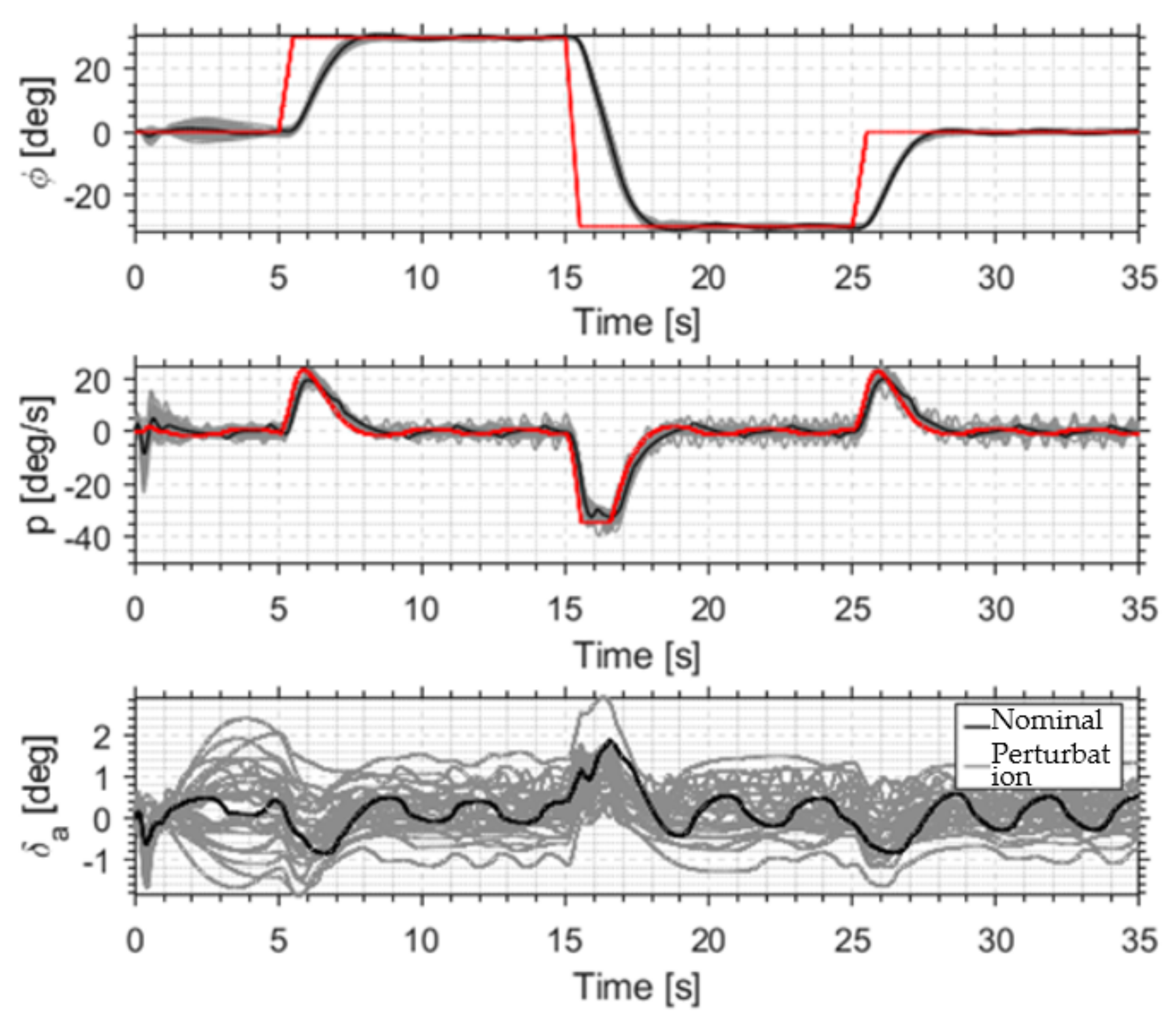
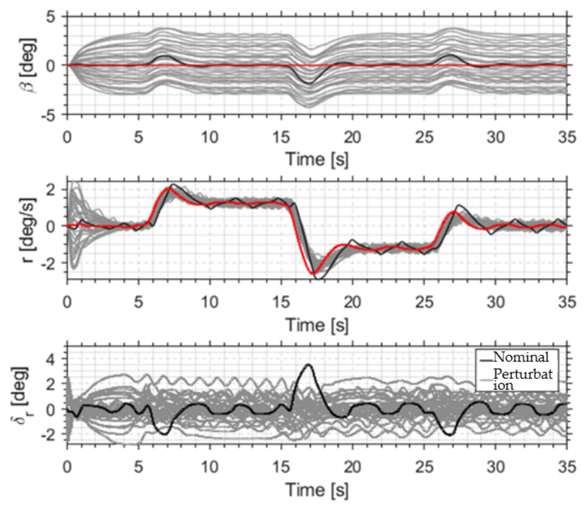
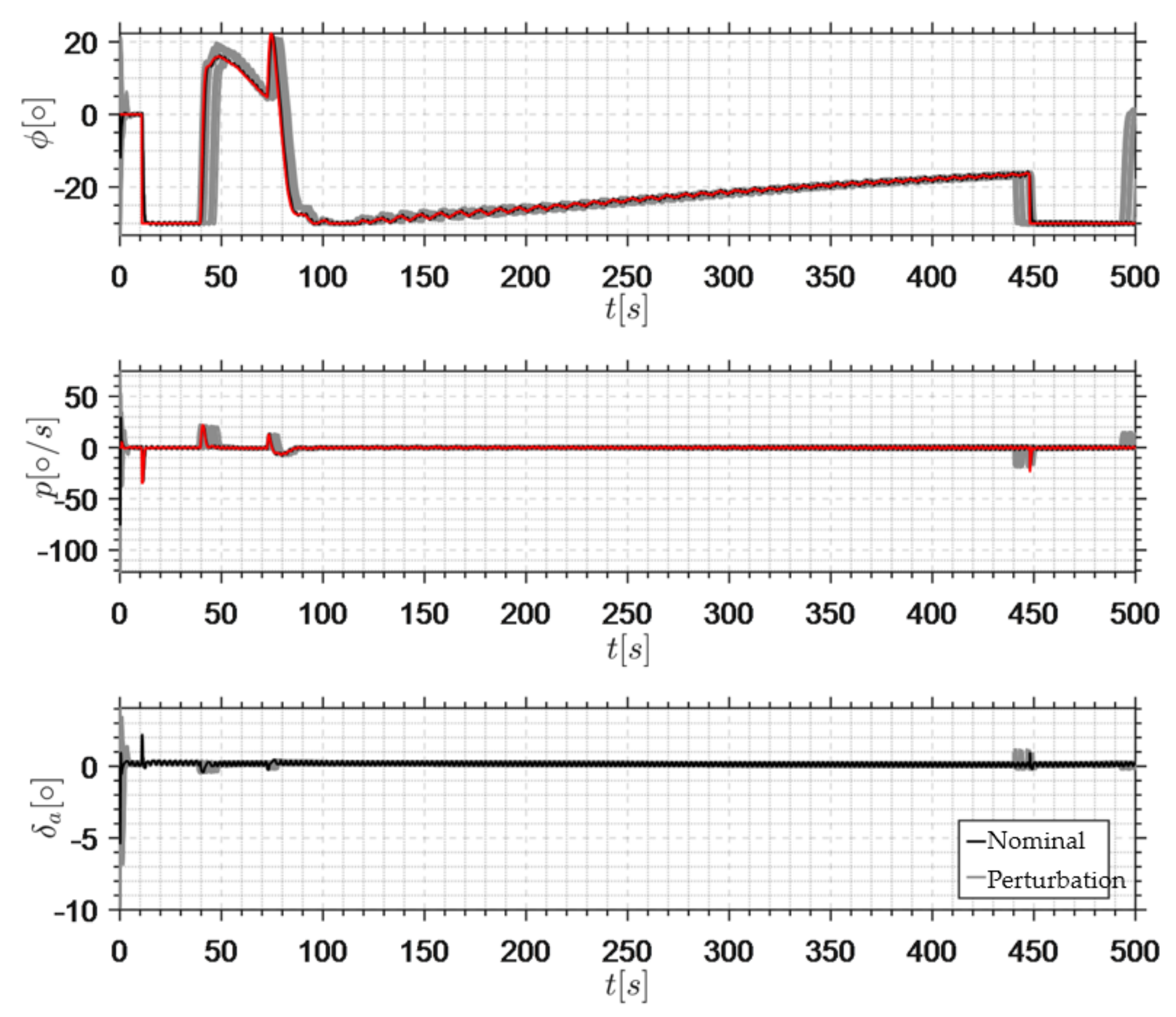
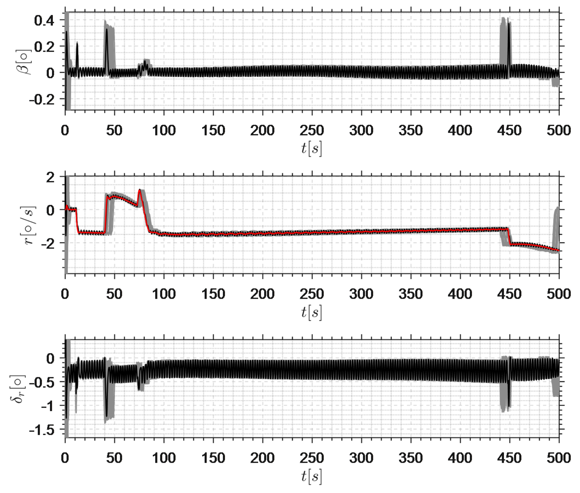
4.2. Perturbation Simulation of Inner Loop Maneuver

Although wind tunnels can in general provide high-quality aerodynamic parameters, a discrepancy between the simulation and real model caused by the experimental equipment and Reynolds number would exist. It was necessary to use the parameter perturbation approach to facilitate a robust verification. Six-degree-of-freedom (6-DOF) dynamics perturbation simulations for robust verification are carried out. The simulation of roll maneuver is conducted at the state points in Table 1, Table 2 and Table 3. The input instructions of roll maneuver are shown in

Table 4. Input instructions for roll maneuver.

Instructions	Simulation Time (Unit: S)
	0	5	5.5	15	15.5	25	25.5	30
Roll angle instruction	0	0	30°	30°	−30°	−30°	0	0
Pitch angle instruction	The pitch angle is the trim angle of attack
Side-slip angle instruction	0

.

The maneuver perturbation range is shown in

Table 5. Parameter perturbation simulation of supersonic task.

Parameter	Uncertainty	Parameter	Uncertainty
rotational inertia	±10%	Derivative of static stability	±20%
Pneumatic rudder control derivative	±20%	Side-slip measurement deviation	±3°
Deviation of center of gravity	±1 cm	Deviation of aircraft flight status at drop time	±5%
Sonic deflection	±15%	Dynamic pressure deflection	±15%
Pitch control derivative deviation	±20%	Pitch damping derivative deviation	±80%
Pitch static stability derivative deviation	±20%	Lift control derivative deviation	±20%
Pitch lift damping derivative deviation	±50%	Lift line slope deviation	±20%
Derivative deviation of side force	±20%	Lateral force control derivative deviation	±20%
Derivative deviation of roll angle velocity side force	±50%	Yaw angular velocity lateral force derivative deviation	±20%
Roll moment static stability derivative deviation	±20%	Aileron control cross derivative deviation	±20%
Roll moment control derivative deviation	±20%	Intercross dynamic derivative deviation	±80%
Rudder control cross derivative deviation	±20%	Yaw damping derivative deviation	±80%
Roll damping derivative deviation	±80%	Aileron rudder surface clearance	0.3°
Intercross dynamic derivative deviation	±80%	Clearance of elevator rudder surface	0.3°
Deviation of static stability derivative of yaw moment	±10%	Clearance of rudder surface	0.3°
Yaw moment control derivative deviation	±30%

. In addition, the Monte-Carlo simulation curves of design points (altitude 1 km, Mach number 0.2), (altitude 9 km, Mach number 0.7), and (altitude 12 km, Mach number 1.2) are shown from Figure 18, Figure 19, Figure 20, Figure 21, Figure 22 and Figure 23. The corresponding test results were obtained by randomly generating 100 combination cases. In Table 5, the LESO-compensated triaxial decoupling control method of roll/pitch/sideslip ensures excellent attitude dynamic quality. In the Monte-Carlo simulation [24], the rising time of the pitch angle is about 2.6 s and remains consistent under model parameter perturbations, which indicates that the designed control law has high quality robustness.

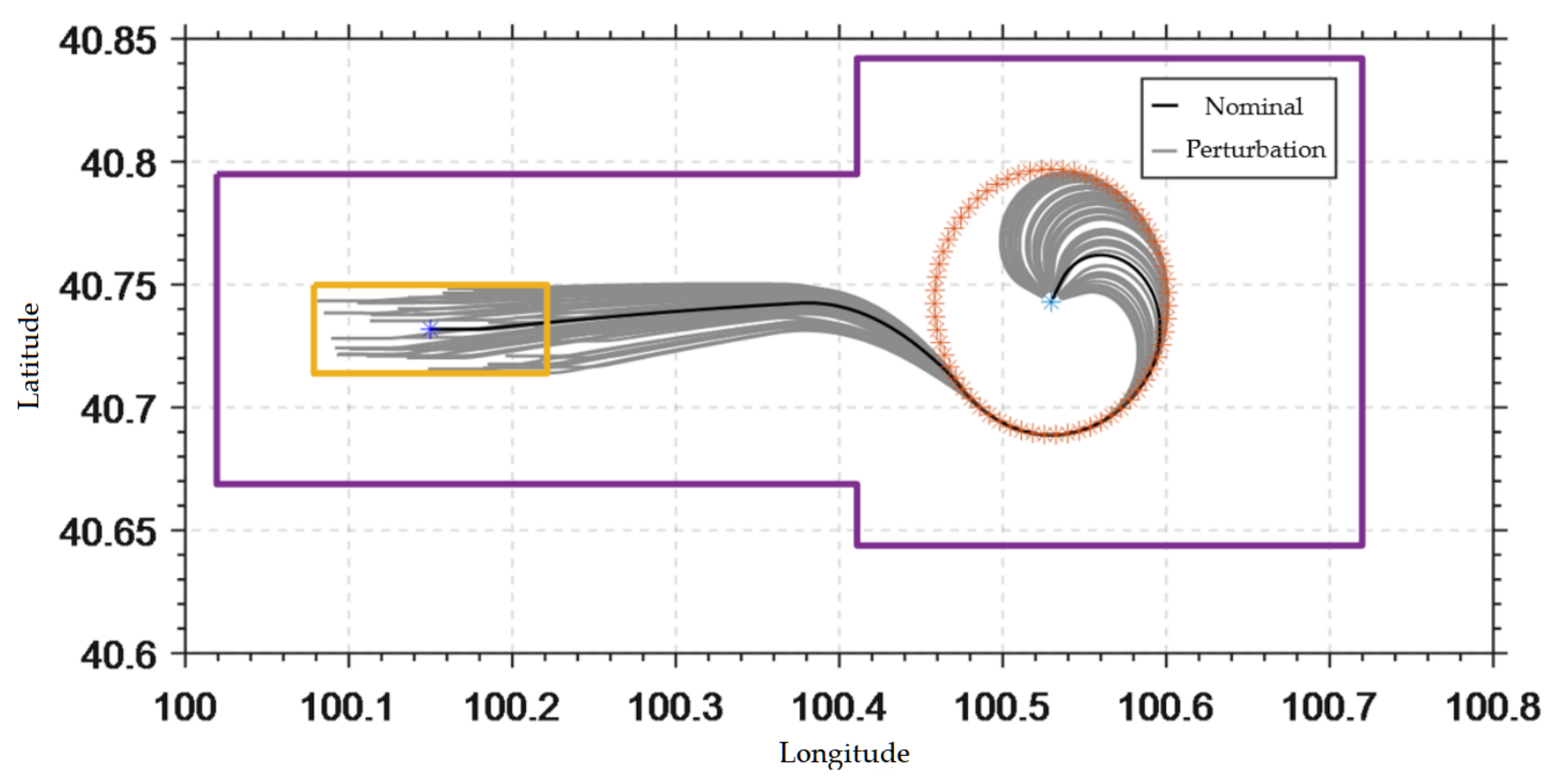
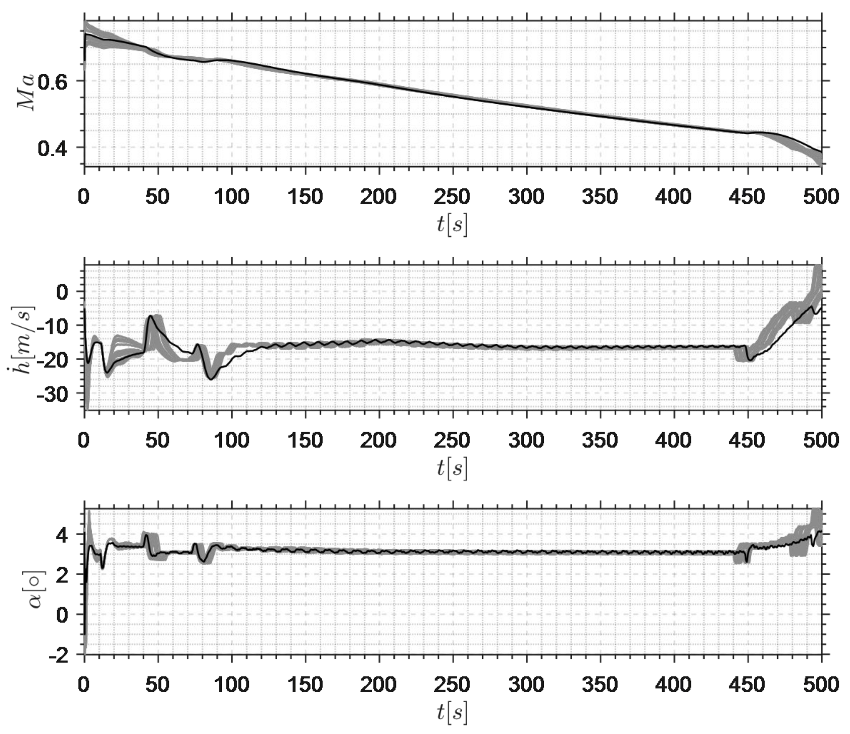
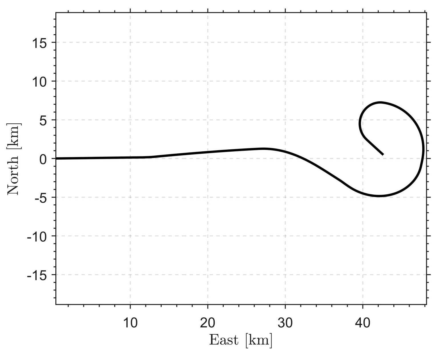
4.3. Simulation Validation

In the full mission simulation, the flight control strategy should have double sets of guidance logic for successful and unsuccessful rocket ignition; the guidance logic for powered flight section and unpowered return section is as follows.

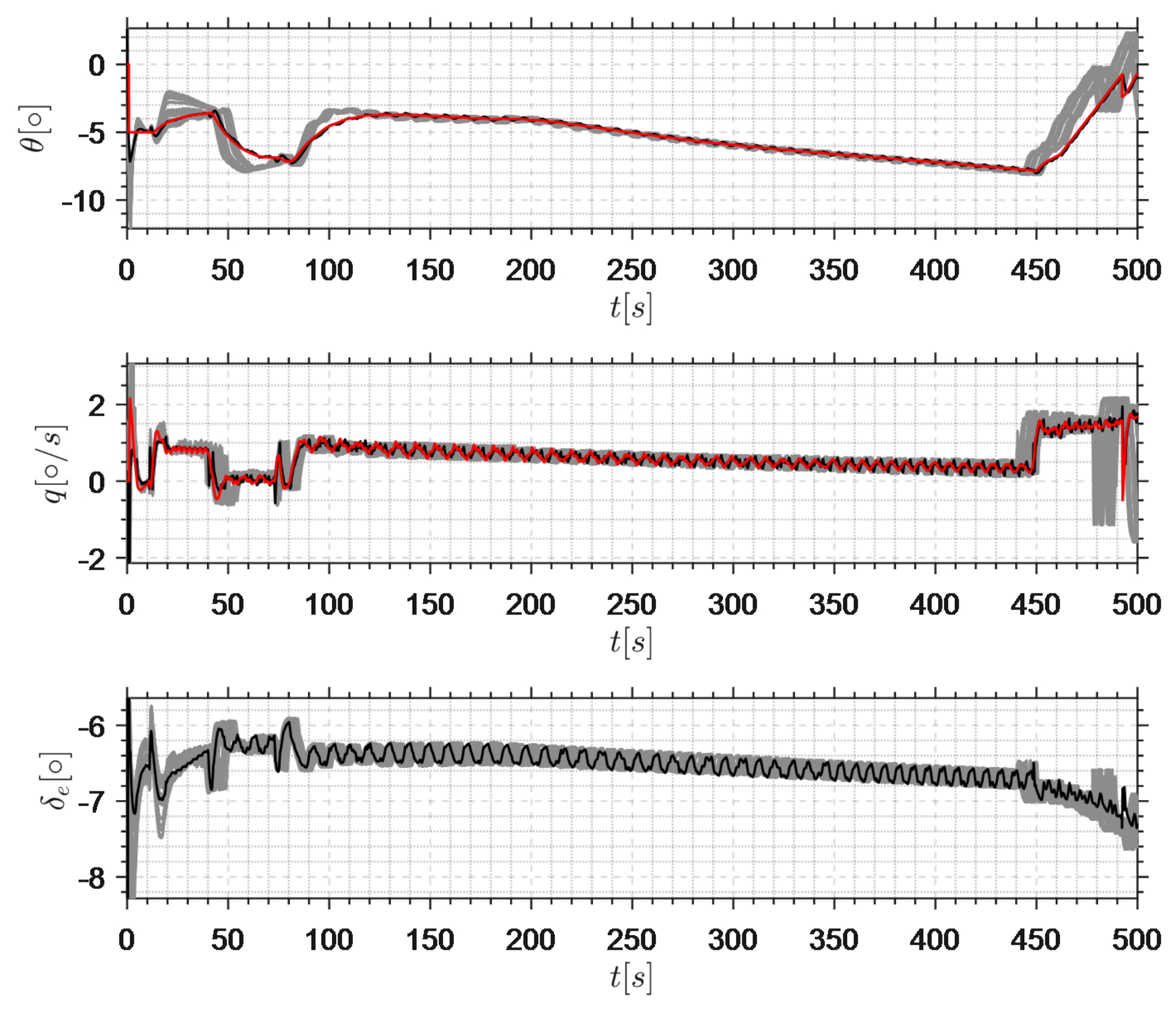
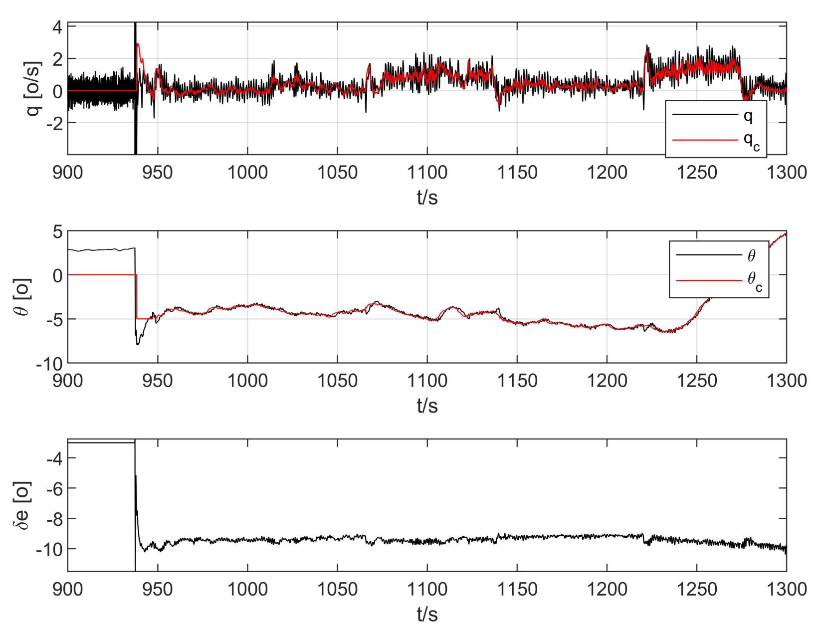
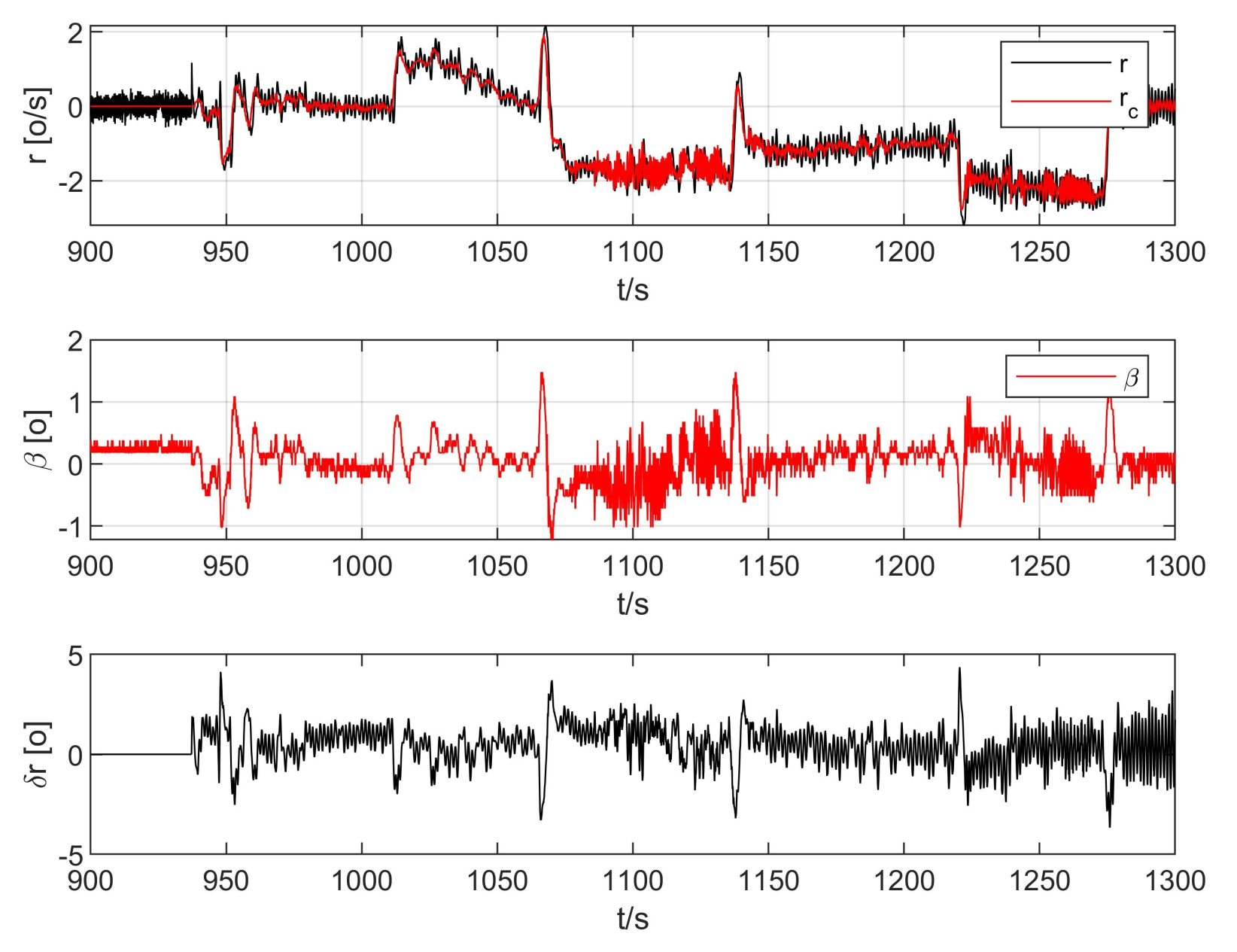
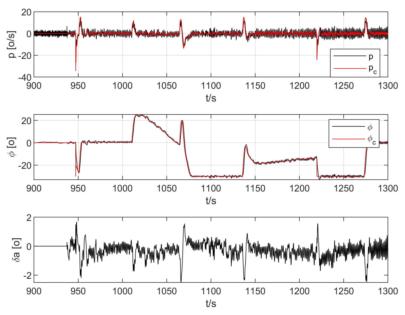
4.3.1. Powered Return Flight

The guidance logic of the airborne release is as follows:

• Longitudinal control pitch angle is −5° (balanced sliding performance);
• Laterally control the roll angle rate to 0°/s in the first second of entering the delivery section. Then, control the roll angle to 0°;
• Longitudinally control the yaw angular rate to 0°/s in the first second of entering the launching section. Then, control the sideslip angle to 0°.

Enter a powered flight section when the following conditions are simultaneously satisfied:

• The current flight path is a powered flight path and enters the launching section for more than 10 s. The roll angle is less than 5°, the pitch angle deviation is less than 5°, and the sideslip angle is less than 5°;

Enter the unpowered return section when one of the following conditions is satisfied:

• The current mission is an unpowered mission and enters the launching section for more than 10 s;
• The current mission is a powered mission and enters the launching section for more than 12 s;

4.3.2. Unpowered Return Flight

In the no-power return section, the longitudinal surface speed was set at 450 km/h, and the lateral approach and entry into the adjustment circle (radius 5 km) were carried out for no-power slide. When the altitude is less than 3.5 km, the energy ratio is calculated. The recovery section is entered when one of the following conditions is met:

• Energy ratio is less than 1.2;
• Height less than 2.5 km.

4.3.3. The Recovery Period

In the recovery section, the laterally guided aircraft is heading to the recovery point, the roll angle limit is 30°, the indicator speed of the longitudinal guided aircraft approaches 350 km/h (indicator speed instruction is adjusted with the waiting flight distance), and the recovery action is performed when one of the following conditions is met:

• The distance is less than 400 m;
• Altitude is less than 1850 m;
• Airspeed is lower than 320 km/h.

The recovery action is the following: after the unmanned aerial vehicle (UAVs) is level, give level instruction 3 s after judging table speed; when the speed is less than 320 km/h, send open umbrella instruction; hair open umbrella instructions are sent after 15 s of open air warehouse; send instructions to open air warehouse 2 s of the rudder surface after zero; send the balloon inflated instruction detected after landing impact (5 g); send umbrella instruction; make a complete recovery.

Now, only the perturbation simulation of flight mission with unsuccessful launch rocket ignition is given. The range of aerodynamic pull and airborne drop separation pull is shown in Table 5. The carrier aircraft was randomly put into the 4 km × 12 km drop area. The wind interference volume was selected as the (1-cos) pulse collision wind and turbulence defined on the body axis, and the west wind of 50 m/s was superimposed at an altitude of 11 km. The corresponding test results were obtained by randomly generating 100 combined cases, as shown in Figure 24, Figure 25, Figure 26, Figure 27 and Figure 28.

The purple wire box in Figure 24 is the no-fly zone, the yellow wire box is the initial drop zone, the red circle is the energy dissipation circle, and the corresponding dotted and black lines are the perturbation and nominal route. The LADRC three-channel decoupling control can guarantee the stability of the attitude. At the same time, in the Monte-Carlo simulation, the narrow envelope of multiple states and high trajectory coincidence indicate the dynamic quality robustness of the designed control system.

4.4. Real-World Validation

Only subsonic real-world flight results were presented. The ICE aircraft was released at a speed of Mach 0.8 and an altitude of 11,000 m. The proposed SISO cascaded ESO-based controller was chosen as the flight control law. A large number of Monte-Carlo simulations were conducted before the real-world flight. Throughout the flight, the bandwidth parameters of ESO were fixed, with the exception of b0, which was scheduled according to Mach number. A free release mission scenario is presented in Figure 29. The attitude tracking performance is shown in Figure 30, Figure 31 and Figure 32. At the initial release phase, the maximum drop pitch angular rate reaches 60°/s. Correspondingly, the maximum pitch angle reaches -8° and the maximum roll angle is 20°. The sideslip angle keeps within 2°. It can be seen that the attitude changes dramatically within a very short in the release phase. Then, the ICE aircraft is guidanced into the energy dissipation circle (radius 5 km). During the mission scenario, the sideslip angle and lateral–directional decoupling control was achieved. As shown in Figure 30, Figure 31 and Figure 32, the bank angle, pitch angle, and sideslip angle were tracked without any steady errors or overshoot, illustrating the precise tracking performance of the roll pitch and yaw angular rate, respectively.

5. Conclusions

This paper mainly studies the disturbance rejection control strategy for a supersonic tailless aircraft. The results are as follows: firstly, the longitudinal stability $\frac{d{C}_m}{d{C}_L}$ varies from −3% to 24% throughout the mission, which poses a challenge to the control law design. Through the Weissman criterion diagram, at a high angle of attack ($\alpha >10°$) of supersonic speed, the aircraft has a large lateral deviation characteristic. Then, the cascaded ADRC attitude control law is designed. Moreover, the timescale-separation turning principle complying with flight quality specification is introduced to realize control gains tuning. Finally, the flight test mission is simulated under nominal conditions, model parameter perturbation, and wind disturbance. The results show that the dynamic performance of the plant under LADRC framework is exceedingly robust and that the designed control law has high quality robustness. The real-world experiment is conducted to verify the effectiveness of the proposed control framework.

References

1. Kroo, I. Aerodynamic concepts for future aircraft. In Proceedings of the 30th Fluid Dynamics Conference, Norfolk, VA, USA, 28 June–1 July 1999. [Google Scholar]
2. Roman, D. Aerodynamic design challenges of the blended-wing-body subsonic transport. In Proceedings of the 18th Applied Aerodynamics Conference, Denver, CO, USA, 14–17 August 2000. [Google Scholar]
3. He, Z.; Hu, J.; Wang, Y.; Cong, J.; Han, L.; Su, M. Sample entropy based prescribed performance control for tailless aircraft. ISA Trans. 2022, 131, 349–366. [Google Scholar] [CrossRef] [PubMed]
4. Rostami, M.; Bardin, J.; Neufeld, D.; Chung, J. A Multidisciplinary Possibilistic Approach to Size the Empennage of Multi-Engine Propeller-Driven Light Aircraft. Aerospace 2022, 9, 160. [Google Scholar] [CrossRef]
5. Zhou, Z.; Huang, J. Hybrid Deflection of Spoiler Influencing Radar Cross-Section of Tailless Fighter. Sensors 2021, 21, 8459. [Google Scholar] [CrossRef] [PubMed]
6. Liu, Z.; Luo, L.; Zhang, B. An Aerodynamic Design Method to Improve the High-Speed Performance of a Low-Aspect-Ratio Tailless Aircraft. Appl. Sci. 2021, 11, 1555. [Google Scholar] [CrossRef]
7. Nie, B.; Liu, Z.; Guo, T.; Fan, L.; Ma, H.; Sename, O. Design and Validation of Disturbance Rejection Dynamic Inverse Control for a Tailless Aircraft in Wind Tunnel. Appl. Sci. 2021, 11, 1407. [Google Scholar] [CrossRef]
8. Liu, L.; Tian, B. Comprehensive Engineering Frequency Domain Analysis and Vibration Suppression of Flexible Aircraft Based on Active Disturbance Rejection Controller. Sensors 2022, 22, 6207. [Google Scholar] [CrossRef] [PubMed]
9. Deng, Z.; Bing, F.; Guo, Z.; Wu, L. Rope-Hook Recovery Controller Designed for a Flying-Wing UAV. Aerospace 2021, 8, 384. [Google Scholar] [CrossRef]
10. Zhang, Q.; Wei, Y.; Li, X. Quadrotor Attitude Control by Fractional-Order Fuzzy Particle Swarm Optimization-Based Active Disturbance Rejection Control. Appl. Sci. 2021, 11, 11583. [Google Scholar] [CrossRef]
11. Huang, L.; Pei, H. Design of Yaw Controller for a Small Unmanned Helicopter Based on Improved ADRC. Guid. Navig. Control 2021, 1, 2140001. [Google Scholar] [CrossRef]
12. Shen, S.; Xu, J. Adaptive neural network-based active disturbance rejection flight control of an unmanned helicopter. Aerosp. Sci. Technol. 2021, 119, 107062. [Google Scholar] [CrossRef]
13. Stevens, B.L.; Lewis, F.L.; Johnson, E.N. Aircraft Control and Simulation: Dynamics, Controls Design, and Autonomous Systems; John Wiley and Sons: Hoboken, NJ, USA, 2015. [Google Scholar]
14. MILF-8785C; Military Specification Flying Qualities of Piloted Airplanes. United States Air Force: Washington, DC, USA, 1991.
15. Wang, Z.; Li, J.; Duan, D. Manipulation strategy of tilt quad rotor based on active disturbance rejection control. Proc. Inst. Mech. Eng. Part G J. Aerosp. Eng. 2020, 234, 573–584. [Google Scholar] [CrossRef]
16. Song, C.; Wei, C.; Yang, F.; Cui, N. High-order sliding mode-based fixed-time active disturbance rejection control for quadrotor attitude system. Electronics 2018, 7, 357. [Google Scholar] [CrossRef] [Green Version]
17. Han, J. Active disturbance rejection controller and its applications. Control Decis. 1998, 13, 19–23. [Google Scholar]
18. Guerrero-Castellanos, J.F.; Durand, S.; Munoz-Hernandez, G.A.; Marchand, N.; Romeo, L.L.G.; Linares-Flores, J.; Mino-Aguilar, G.; Guerrero-Sánchez, W.F. Bounded Attitude Control with Active Disturbance Rejection Capabilities for Multirotor UAVs. Appl. Sci. 2021, 11, 5960. [Google Scholar] [CrossRef]
19. Zhuang, H.; Sun, Q.; Chen, Z.; Zeng, X. Back-stepping Active Disturbance Rejection Control for Attitude Control of Aircraft Systems Based on Extended State Observer. Int. J. Control Autom. Syst. 2021, 19, 2134–2149. [Google Scholar] [CrossRef]
20. Mei, D.; Yu, Z.Q. Active disturbance rejection control strategy for airborne radar stabilization platform based on cascade extended state observer. Assem. Autom. 2020, 40, 613–624. [Google Scholar] [CrossRef]
21. Gao, Z. Scaling and bandwidth-parameterization based controller tuning. In Proceedings of the American Control Conference, Minneapolis, MN, USA, 14–16 June 2006; Volume 6. [Google Scholar]
22. Kong, S.; Sun, J.; Qiu, C.; Wu, Z.; Yu, J. Extended State Observer-Based Controller With Model Predictive Governor for 3-D Trajectory Tracking of Underactuated Underwater Vehicles. IEEE Trans. Ind. Inform. 2021, 17, 6114–6124. [Google Scholar] [CrossRef]
23. Luo, S.; Sun, Q.; Sun, M.; Tan, P.; Wu, W.; Sun, H.; Chen, Z. On decoupling trajectory tracking control of unmanned powered parafoil using ADRC-based coupling analysis and dynamic feedforward compensation. Nonlinear Dyn. 2018, 92, 1619–1635. [Google Scholar] [CrossRef]
24. Olsson, A.M.J.; Sandberg, G.E. Latin hypercube sampling for stochastic fifinite element analysis. J. Eng. Mech. 2002, 128, 121–125. [Google Scholar]
Figure 1. The mission is divided into four phases: (a) the launching separation phase; (b) the powered flight phase; (c) the gliding phase; (d) the recovery phase.
Aerospace 10 00198 g001
Figure 2. ICE aircraft flight envelope and nominal path: Map the flight trajectory to the height-mach profile so that we can select the design point.
Aerospace 10 00198 g002
Figure 3. The configuration of ICE aircraft control surface.
Aerospace 10 00198 g003
Figure 4. Longitudinal static stability along the flight trajectory.
Aerospace 10 00198 g004
Figure 5. The diagram of Weissman criterion. Area A is the no-deviation area. Area B is the slight deviation area. Area C is a moderate deviation area. Area D is strong deviation divergence area. Area E is the moderate yaw divergence area. Area F is the strong divergence area.
Aerospace 10 00198 g005
Figure 6. Complete control architecture. Cascaded ESO-based control schemes to handle the control stabilization.
Aerospace 10 00198 g006
Figure 7. Complete EOS-based control architecture. Note that b (for p , q , r ) describes control efficiency related parameter. β 1 and β 2 (for p , q , r ) are ESO ralated parmeters. δ (for a , e , r ) is the actuator command. k (for p , q , r ) defines low-speed outer loop parameter. f (for p , q , r ) is lumped disturbance of angular rate loop.
Aerospace 10 00198 g007
Figure 8. The structure of yaw angular rate loop control.
Aerospace 10 00198 g008
Figure 9. The structure of yaw angular rate loop control.
Aerospace 10 00198 g009
Figure 10. Open-loop Bode diagram at elevator of sideslip angle control loop.
Aerospace 10 00198 g010
Figure 11. Loop Bode diagram of sideslip angle control loop.
Aerospace 10 00198 g011
Figure 12. Measurement of noise amplitude-frequency.
Aerospace 10 00198 g012
Figure 13. Measurementof noise phase frequency.
Aerospace 10 00198 g013
Figure 14. The flow of control law gain.
Aerospace 10 00198 g014
Figure 15. The Nichols diagram of pitch rate loop.
Aerospace 10 00198 g015
Figure 16. The Nichols diagram of pitch rate loop breaking at elevator.
Aerospace 10 00198 g016
Figure 17. Step response of pitch channel.
Aerospace 10 00198 g017
Figure 18. Perturbation simulation of the roll channel at 1 km altitude and 0.2 Mach number.
Aerospace 10 00198 g018
Figure 19. Perturbation simulation of the directional channel at 1 km altitude and 0.2 Mach number.
Aerospace 10 00198 g019
Figure 20. Perturbation simulation of the roll channel at 9 km altitude and 0.7 Mach number.
Aerospace 10 00198 g020
Figure 21. Perturbation simulation of the roll channel at 9 km altitude and 0.7 Mach number.
Aerospace 10 00198 g021
Figure 22. Perturbation simulation of rolling channel at 12 km altitude and 1.2 Mach number.
Aerospace 10 00198 g022
Figure 23. Perturbation simulation of rolling channel at 12 km altitude and 1.2 Mach number.
Aerospace 10 00198 g023
Figure 24. Perturbation simulation of lateral position during the mission.
Aerospace 10 00198 g024
Figure 25. Perturbation simulation of pitch channel during the gliding phase.
Aerospace 10 00198 g025
Figure 26. Perturbation simulation of unpowered return rolling channel.
Aerospace 10 00198 g026
Figure 27. Perturbation simulation of yaw channel during flight mission.
Aerospace 10 00198 g027
Figure 28. Perturbation simulation of height channel during flight mission.
Aerospace 10 00198 g028
Figure 29. Flight trajectory of the flight mission.
Aerospace 10 00198 g029
Figure 30. Flight test data. Command and response value of the pitch channel.
Aerospace 10 00198 g030
Figure 31. Flight test data. Command and response value of the yaw channel.
Aerospace 10 00198 g031
Figure 32. Flight test data. Command and response value of the roll channel.
Aerospace 10 00198 g032