Attitude Dynamics of Spinning Magnetic LEO/VLEO Satellites

Abstract

With the growing popularity of small satellites, the interaction with the air in low and especially in very low Earth orbits becomes a significant resource for passive angular stabilisation. However, the possibility of spin motion remains a considerable challenge for missions involving aerodynamically stabilised satellites. The goal of this paper was to investigate the attitude motion of arbitrarily spinning satellites in LEO and VLEO under the action of aerodynamic, gravitational, and magnetic torques, taking into account the aerodynamic damping. Using an umbrella-shaped deployable satellite as an example, the study demonstrated that both regular and chaotic attitude regimes are possible in the attitude motion. The occurrence of chaos was verified by means of Poincaré sections. The results revealed that, to prevent chaotic motion, active attitude control and reliable deployment techniques for aerodynamically stabilised satellites are needed.

1. Introduction

If a satellite is in LEO or very low Earth orbit (VLEO) (typically characterised by altitudes of 80–450 km), its interaction with the atmosphere needs to be taken into account [1,2,3,4]. Aerodynamic torque resulting from this interaction can be used for angular stabilisation. Passive aerodynamic stabilisation is the simplest, since it does not require any power supply. This type of stabilisation has been studied since the late 1950s [5,6,7,8,9]. Currently, with the growing popularity of small satellites, which are more sensitive to the interaction with the air, the number of missions using partial or total aerodynamic stabilisation has increased substantially. Current research in this field is focused on atmosphere-breathing electric propulsion systems [10,11]; satellite shape optimisation and drag reduction [12,13,14]; using aerodynamic forces for formation flying control [15,16]; and creating variable shapes in order to change satellite equilibrium positions [17]. Another popular topic related to aerodynamic stabilisation is the design of re-entry capsules [18,19,20,21,22] and their systems [23].

In the general case, aerodynamically stabilised satellites may spin relative to an orbiting reference frame. A recent in-orbit test [19] of an inflatable satellite showed that this spinning may be caused by distortion of the aeroshell after its deployment. Regardless of the cause of spinning, the joint action of the environmental and gyroscopic torques produces several equilibrium angular positions, which can be either stable or unstable. The classical papers by Meirovitch, Wallace, and Frik [6], regarding spatial attitude motion, dealt only with two environmental torques, namely gravitational and aerodynamic, both depending only on the satellite’s orientation. More recent studies have considered other possible perturbations, such as orbit eccentricity [24], resisting medium [25,26], inertial torques due to elastic elements [27,28,29,30], and magnetic [31,32,33] and damping aerodynamic torques [2,30,33], demonstrating that, in the presence of unstable equilibrium positions, these perturbations may lead to chaos. Most of these papers, aimed at studying chaos in the attitude motion, were focused on the limiting case of planar pitch motion or did not simultaneously take into account magnetic and aerodynamic torques.

The goal of this paper was thus to investigate the attitude motion of arbitrarily spinning satellites in LEO and VLEO under the action of aerodynamic, gravitational, and magnetic torques, taking into account the aerodynamic damping. In order to achieve this goal, the unperturbed and perturbed motions are defined, the equations of motion were derived, the equilibrium positions were found, and a case study dealing with a deployable LEO/VLEO satellite was considered.

The paper has the following structure. In Section 2, the problem of satellite attitude motion under several environmental torques is formulated and the expressions for the torques and their potential functions are considered. Section 3 presents the definitions of the unperturbed and perturbed motions and the derivation of the equations of motion. In addition, the equilibrium positions for the unperturbed motion are found by analysing the dynamic potential. Section 4 is devoted to the case study of the attitude motion of a deployable satellite in LEO and VLEO. Finally, the conclusions are given in Section 5.

2. Problem Statement

The attitude motion of the satellite is considered under the following assumptions:

• The orbit of the satellite remains circular.
• The atmosphere is not rotating.
• The density and temperature of the incident air stream are chosen using the Jacchia–Bowman 2008 Atmosphere Model [34].
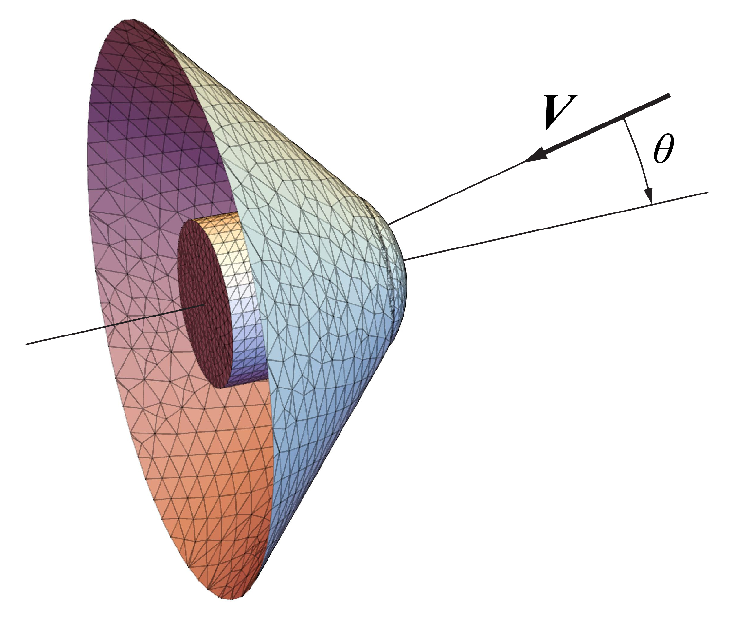
• The satellite is shaped as a body of revolution.
• The centre of mass of the satellite lies on its axis of symmetry.
• The transverse moments of inertia of the satellite are equal to each other.

The last two assumptions define the inertia matrix of the satellite:

$$J=\left(\begin{array}{ccc}A& 0& 0\\ 0& C& 0\\ 0& 0& C\end{array}\right)$$

(1)

where A is the longitudinal moment of inertia, i.e., about the axis of symmetry of the satellite, and C is the moment of inertia about the axes perpendicular to the axis of symmetry.

2.1. Coordinate Systems

The following coordinate systems or reference frames, denoted using a convenient notation proposed in [35], are used:

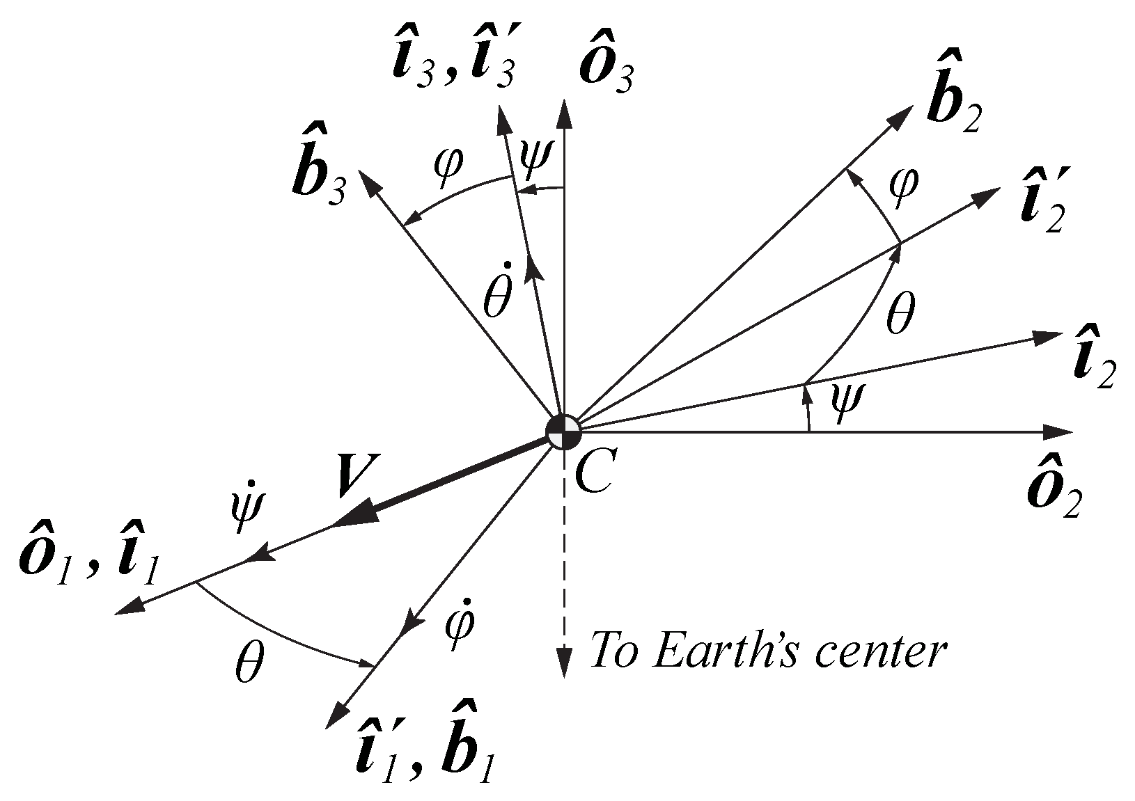
• The orbital frame O is defined through an orthonormal right-hand set of unit vectors ${\widehat{\mathit{o}}}_k$, $k=1,2,3$ with an origin at the satellite’s centre of mass (Figure 1). The ${\widehat{\mathit{o}}}_1$ vector is tangential to the orbit in the flight direction, the ${\widehat{\mathit{o}}}_3$ vector is directed along the radius vector from the centre of the Earth to the centre of mass of the satellite.
• The body-fixed frame B is defined through a set ${\widehat{\mathit{b}}}_k$. These vectors coincide with the satellite’s principal axes of inertia, and the ${\widehat{\mathit{b}}}_1$ vector lies along the axis of symmetry. The orientation of ${\widehat{\mathit{b}}}_k$ relative to ${\widehat{\mathit{o}}}_k$ is described by a symmetric $(1,3,1)$ set of Euler angles corresponding to three successive positive rotations: first about Axis 1 by the precession angle $\psi$, then about Axis 3 by the nutation angle $\theta$ (angle of attack), $0\le \theta \le \pi$, and finally, about Axis 1 by the spin angle $\phi$, as is shown in Figure 1. The transformation matrix $\mathsf{\Theta }$ between O and B is defined by

  $${\mathit{v}}^B=\mathsf{\Theta }{\mathit{v}}^O$$

  (2)

  where

  $$\mathsf{\Theta }=\left(\begin{array}{ccc}c\theta & c\psi s\theta & s\theta s\theta \\ -c\phi s\theta & c\theta c\phi c\psi -s\phi s\psi & c\psi s\phi +c\theta c\phi s\psi \\ s\theta s\phi & -c\theta c\psi s\phi -c\phi s\psi & c\phi c\psi -c\theta s\phi s\psi \end{array}\right),$$

  (3)
  $c\theta =cos\theta$, $s\theta =sin\theta$, etc.
• The intermediate coordinate frames I and $I^{\prime }$ are defined through unit vector sets ${\widehat{\mathit{i}}}_k$, ${{\widehat{\mathit{i}}}^{\prime }}_k$, respectively. The orientations of these frames relative to the orbital frame are determined by the above-mentioned rotations: a single rotation by the angle $\psi$ for the ${\widehat{\mathit{i}}}_k$ frame and two successive rotations by the angles $\psi$ and $\theta$ for the ${{\widehat{\mathit{i}}}^{\prime }}_k$ frame.

Note that the satellite’s attitude can be described not only by Euler angles, but also quaternions, Cayley–Klein parameters, etc. [35,36]. In this paper, Euler angles were used, since, in the authors’ opinion, they give the clearest physical picture of the considered problem.

2.2. Environmental Torques

The following environmental torques were considered: gravitational, magnetic, and aerodynamic, the last one consisting of restoring and damping torques. For the convenience of the analysis, it is useful to separate the conservative torques from non-conservative ones. Any torque $\mathit{M}$ acting on the body is conservative, if it depends only on the body’s orientation and its curl is equal to zero [8]:

$$\begin{array}{c}{\displaystyle \frac{\partial M_{\phi }}{\partial \theta }}-{\displaystyle \frac{\partial M_{\theta }}{\partial \phi }}=0,\hfill \\ {\displaystyle \frac{\partial M_{\psi }}{\partial \phi }}-{\displaystyle \frac{\partial M_{\phi }}{\partial \psi }}=0,\hfill \\ {\displaystyle \frac{\partial M_{\theta }}{\partial \psi }}-{\displaystyle \frac{\partial M_{\psi }}{\partial \theta }}=0\hfill \end{array}$$

(4)

where

$$\begin{array}{ccc}{M}_{\psi }={\left.\mathit{M}·{\widehat{\mathit{o}}}_1\right|}_{\theta =0,\phi =0},& M_{\theta }={\left.\mathit{M}·{\widehat{\mathit{i}}}_3\right|}_{\phi =0},& M_{\phi }=\mathit{M}·{{\widehat{\mathit{i}}}^{\prime }}_1.\end{array}$$

(5)

If a torque satisfies Condition (4), it has a potential function, which can be found as

$$V=-\underset{0}{\overset{\psi }{\int }}{M}_{\psi }d\psi -\underset{0}{\overset{\theta }{\int }}{M}_{\theta }d\theta -\underset{0}{\overset{\phi }{\int }}{M}_{\phi }d\phi .$$

(6)

Further in this subsection, we will derive, if possible, the potential functions for each of the environmental torques considered.

2.2.1. Gravitational Torque

The torque due to the gravity gradient is defined as [7]

$${\mathit{M}}_G=3{\mathsf{\Omega }}^2\left({\widehat{\mathit{o}}}_3\times J{\widehat{\mathit{o}}}_3\right)$$

(7)

where $\mathsf{\Omega }=\sqrt{{\mu }_G/R_0^3}$ is the mean motion, $R_0=R_e+h$ is the orbit radius, $R_e$ is the mean radius of the Earth, h is the orbital altitude, and ${\mu }_G$ is the gravitational parameter of the Earth. According to Equation (5), the projections of the vector ${\mathit{M}}_G$ on the (1,3,1) axes ${\widehat{\mathit{o}}}_1,{\widehat{\mathit{i}}}_3,{{\widehat{\mathit{i}}}^{\prime }}_1$ (Figure 1) are, respectively,

$$\begin{array}{c}{M}_{G_{\psi }}=0,\hfill \\ M_{G_{\theta }}={\displaystyle \frac{3}{2}}\left(C-A\right){\mathsf{\Omega }}^2{sin}^2\psi sin2\theta ,\hfill \\ M_{G_{\phi }}=0.\hfill \end{array}$$

(8)

The potential energy corresponding to the gravitational torque can be obtained by the substitution of Equation (8) into Equation (6). Using a well-known double-angle formula after the integration and omitting constant terms, we can write the potential energy in the form:

$$V_G=-\underset{0}{\overset{\theta }{\int }}{M}_{\theta }d\theta =-{\displaystyle \frac{3}{2}}\left(C-A\right){\mathsf{\Omega }}^2{sin}^2\theta {sin}^2\psi .$$

(9)

which, for the chosen Euler angles, is symmetric with respect to the angles $\theta$ and $\psi$.

2.2.2. Magnetic Torque

The magnetic torque acting on a satellite is [37]

$${\mathit{M}}_M=\mu \times \mathit{B}$$

(10)

where $\mu$ is the vector of the satellite’s own magnetic moment:

$$\mu ={\left(\begin{array}{c}{M}_1\\ M_2\\ M_3\end{array}\right)}^B=\mu {\left(\begin{array}{c}{\overline{M}}_1\\ {\overline{M}}_2\\ {\overline{M}}_3\end{array}\right)}^B,$$

(11)

${\overline{M}}_k=M_k/\mu$ are dimensionless components of the satellite’s own magnetic moment, $\mathit{B}$ is the Earth’s magnetic field, which is modelled as a field of a dipole placed in the centre of the Earth [7]:

$$\mathit{B}={\displaystyle \frac{{\mu }_0{\mu }_m}{4\pi R_0^3}}\left[3{\widehat{\mathit{o}}}_3\left({\mathit{k}}_e·{\widehat{\mathit{o}}}_3\right)-{\mathit{k}}_e\right]$$

(12)

where ${\mathit{k}}_e$ is the dipole direction assumed to be aligned with the Earth’s rotation axis, ${\mu }_0$ is the magnetic permeability of free space, and ${\mu }_m$ is the geomagnetic dipole moment. The magnetic field takes its simplest form if it is expressed in the orbital frame:

$$\mathit{B}={\displaystyle \frac{{\mu }_0{\mu }_m}{4\pi R_0^3}}{\left(\begin{array}{c}-cos\nu sini\\ -cosi\\ 2sinisin\nu \end{array}\right)}^O$$

(13)

In Equation (13), i is the orbital inclination and $\nu$ is the true anomaly:

$$\nu =\mathsf{\Omega }t.$$

(14)

Note, since the magnetic torque is time-dependent for non-equatorial orbits, it is not conservative in general and, thus, has no potential function.

2.2.3. Restoring Aerodynamic Torque

In this paper, the restoring aerodynamic torque is understood as a torque that depends only on the orientation of the body-fixed frame with respect to the flow vector. This orientation is described by two angles, namely the angle of attack $\theta$ and the spin angle $\phi$. Thus, the restoring aerodynamic torque is independent of the precession angle $\psi$. In this case, the conditions (4) for the torque to be conservative are as follows [8]:

$$M_{\psi }=const,$$

(15)

$${\displaystyle \frac{\partial M_{\phi }}{\partial \theta }}={\displaystyle \frac{\partial M_{\theta }}{\partial \phi }}.$$

(16)

For all bodies of revolution with the centre of mass lying on the axis of geometric symmetry, the aerodynamic restoring torque about the longitudinal symmetry axis is equal to zero, so Conditions (15) and (16) become

$$M_{\psi }=M_{\phi }=0,$$

(17)

$${\displaystyle \frac{\partial M_{\theta }}{\partial \phi }}=0.$$

(18)

Thus, for a body of revolution with the centre of mass on the axis of geometric symmetry, the restoring aerodynamic torque is fully described by the function $M_{\theta }=f\left(\theta \right)$. This function can be written in the following form:

$$M_{\theta }=c_r{\overline{M}}_{\theta }$$

(19)

where

$$c_r={\displaystyle \frac{\rho V^2}{2}}{A}_r{L}_r,$$

(20)

$V=\mathsf{\Omega }{R}_0$ is the orbital speed, $A_r$ is the reference area, $L_r$ is the reference length, and $\rho$ is the density of the atmosphere. The restoring aerodynamic torque coefficient ${\overline{M}}_{\theta }$ is a periodic odd function, so it can be approximated by a finite number of terms of a Fourier sine series:

$${\overline{M}}_{\theta }=\sum _{i=1}^n{b}_{i}sini\theta$$

(21)

where n is the number of harmonics. Substituting Equations (17), (19), and (21) into Equation (6), we obtain the potential energy corresponding to the restoring aerodynamic torque:

$$V_A=-\underset{0}{\overset{\theta }{\int }}{M}_{\theta }d\theta =c_r\sum _{i=1}^n{\displaystyle \frac{1}{i}}{b}_{i}cosi\theta .$$

(22)

2.2.4. Damping Aerodynamic Torque

The second component of the aerodynamic torque, which depends not only on the orientation of the body, but also on its angular velocity, is often called the damping torque. In the body-fixed frame B, it can be expressed as [38]

$${\mathit{M}}_d=c_d{\left(\begin{array}{c}{\overline{M}}_1^{{\omega }_1}{\omega }_1\\ {\overline{M}}_2^{{\omega }_2}{\omega }_2\\ {\overline{M}}_3^{{\omega }_3}{\omega }_3\end{array}\right)}^B$$

(23)

where

$$c_d={\displaystyle \frac{\rho V}{2}}{A}_r{L}_r^2,$$

(24)

where ${\overline{M}}_k^{{\omega }_k}={\overline{M}}_k^{{\omega }_k}(\theta ,\psi )$, $k=1,2,3$ are the damping torque coefficients associated with the projections ${\omega }_k$ of the angular velocity vector $\mathbf{\omega }$,

$$\mathbf{\omega }=\left(\begin{array}{c}{\omega }_1\\ {\omega }_2\\ {\omega }_3\end{array}\right)={\left(\begin{array}{c}\dot{\phi }+\dot{\psi }c\theta +\mathsf{\Omega }c\psi s\theta \\ \dot{\theta }s\phi -\dot{\psi }c\phi s\theta +\mathsf{\Omega }\left(c\theta c\phi c\psi -s\phi s\psi \right)\\ \dot{\theta }c\phi +\dot{\psi }s\theta s\phi -\mathsf{\Omega }\left(c\theta c\psi s\phi +s\psi c\phi \right)\end{array}\right)}^B$$

(25)

on the body axes ${\widehat{\mathit{b}}}_k$ [35]. The “longitudinal” damping torque coefficient ${\overline{M}}_1^{{\omega }_1}$ of a body of revolution is an even periodic function of the angle of attack alone, so it can be represented as a Fourier cosine series of a single variable. The “transverse” damping torque coefficients ${\overline{M}}_2^{{\omega }_2}$, ${\overline{M}}_3^{{\omega }_3}$ are even periodic functions of both the angle of attack $\theta$ and the spin angle $\phi$, so they need to be represented as 2D Fourier cosine series. Moreover, due to the axial symmetry of the body, ${\overline{M}}_3^{{\omega }_3}$ is equal to ${\overline{M}}_2^{{\omega }_2}$, calculated for $\phi$ increased or decreased by $\pi /2$. Bearing all these facts in mind, one can write the damping torque coefficients as

$$\begin{array}{c}{\overline{M}}_1^{{\omega }_1}\left(\theta \right)={\displaystyle \sum _{i=0}^m}{a}_{1,i}cosi\theta ,\hfill \\ {\overline{M}}_2^{{\omega }_2}(\theta ,\phi )={\displaystyle \sum _{i=0}^p}{\displaystyle \sum _{j=0}^r}{a}_{2,i,j}cosi\theta cosj\phi ,\hfill \\ {\overline{M}}_3^{{\omega }_3}(\theta ,\phi )={\displaystyle \sum _{i=0}^p}{\displaystyle \sum _{j=0}^r}{a}_{2,i,j}cosi\theta cosj(\phi +\pi /2)={\overline{M}}_2^{{\omega }_2}(\theta ,\phi +\pi /2)\hfill \end{array}$$

(26)

where m, p, and r are the numbers of harmonics. Note that, since, by virtue of Equation (23), the damping aerodynamic torque depends on the angular velocity of the satellite, it has no potential function.

3. Equations of Motion

The attitude motion of aerodynamically stabilised satellites may be treated using the general principles of the analytical mechanics of a rigid body rotating about its centre of mass [36,39,40]. The equations of motion of the satellite are first derived in standard dimensional form using the Euler angles $\psi$, $\theta$, and $\phi$ as generalised coordinates:

$$q={\left(\begin{array}{ccc}\theta & \psi & \phi \end{array}\right)}^T$$

(27)

considering $q_k$ as functions of time. Then, the equations are transformed into dimensionless form, using the true anomaly $\nu$ as the independent variable. This allows simplifying the expressions and investigating the behaviour of the system in an arbitrary space of parameters.

If some torques acting on the satellite are conservative, it is extremely useful for an intuitive analysis of possible satellite motions to define the perturbed and the unperturbed motions. The perturbed motion is defined as the attitude motion of the satellite under the action of all the environmental torques considered in the previous section. Then, the unperturbed motion is the motion of the satellite under the aerodynamic restoring torque and gravitational torque. Both of them are conservative, which justifies the choice of the Lagrangian approach for the derivation of the equations.

3.1. Unperturbed Motion

The kinetic energy of the satellite is

$$T={\displaystyle \frac{1}{2}}\left(A{{\omega }_1}^2+C({{\omega }_2}^2+{{\omega }_3}^2)\right).$$

(28)

After the substitution of the components of the vector $\mathbf{\omega }$, defined by Equation (25), Equation (28) takes the form:

$$T={\displaystyle \frac{1}{2}}A{\left(\dot{\phi }+\dot{\psi }c\theta +\mathsf{\Omega }c\psi s\theta \right)}^2+{\displaystyle \frac{1}{2}}C\left({\dot{\theta }}^2+{\left(\mathsf{\Omega }c\theta c\psi -\dot{\psi }s\theta \right)}^2-2\mathsf{\Omega }\dot{\theta }s\psi +{\mathsf{\Omega }}^2{s}^2\psi \right).$$

(29)

The potential energy is the sum of the gravitational and aerodynamic potential energies:

$$V=V_G+V_A$$

(30)

where $V_G$ and $V_A$ are defined by Equations (9) and (22), respectively. The Lagrangian of the system is

$$\begin{array}{c}L=T-V=\hfill \\ {\displaystyle \frac{1}{2}}A{\left(\dot{\phi }+\dot{\psi }c\theta +\mathsf{\Omega }c\psi s\theta \right)}^2+{\displaystyle \frac{1}{2}}C\left({\dot{\theta }}^2+{\left(\mathsf{\Omega }c\theta c\psi -\dot{\psi }s\theta \right)}^2-2\mathsf{\Omega }\dot{\theta }s\psi +{\mathsf{\Omega }}^2{s}^2\psi \right)-V(\theta ,\psi ).\hfill \end{array}$$

(31)

Since the generalised coordinate $\phi$ does not appear in the Lagrangian, the unperturbed motion has an integral in the form:

$$p_{\phi }=const$$

(32)

where

$$p_{\phi }={\displaystyle \frac{\partial L}{\partial \dot{\phi }}}=A\left(\dot{\phi }+\dot{\psi }c\theta +\mathsf{\Omega }c\psi s\theta \right).$$

(33)

Since the Lagrangian (31) is not an explicit function of time, the Hamiltonian of the system is also an integral of motion. It can be found as

$$\begin{array}{c}H={\displaystyle \sum _{k=1}^2}{\displaystyle \frac{\partial R}{\partial q_k}}{\dot{q}}_k-R=\hfill \\ {\displaystyle \frac{1}{2}}C\left({\dot{\theta }}^2+{\dot{\psi }}^2{s}^2\theta \right)-{\displaystyle \frac{1}{2}}C{\mathsf{\Omega }}^2\left(c^2\theta c^2\psi +s^2\psi \right)+{\displaystyle \frac{p_{\phi }^2}{2A}}-p_{\phi }\mathsf{\Omega }c\psi s\theta +V(\theta ,\psi )=const\hfill \end{array}$$

(34)

where R is the Routhian of the system:

$$R=L-p_{\phi }\dot{\phi }.$$

(35)

The general form of the equations of the unperturbed motion is

$$\begin{array}{c}{\displaystyle \frac{d}{dt}}{\displaystyle \frac{\partial R}{\partial {\dot{q}}_k}}-{\displaystyle \frac{\partial R}{\partial q_k}}=0,k=1,2,\hfill \\ {\dot{p}}_{\phi }=0.\hfill \end{array}$$

(36)

According to Equation (27), the first two of Equation (36) correspond to the non-cyclic coordinates $\psi$ and $\theta$, respectively, while the third of Equation (36) corresponds to the cyclic coordinate $\phi$. The equations of unperturbed motion in dimensionless form can be obtained by solving Equation (36) for ${\ddot{q}}_k$ and dividing both sides of each equation by $A{\mathsf{\Omega }}^2$:

$$\begin{array}{c}\gamma {\psi }^{″}=\left(4\gamma -3\right)s\psi c\psi +\beta \left({\theta }^{\prime }-s\psi \right)csc\theta -2\gamma {\theta }^{\prime }\left(c\psi +{\psi }^{\prime }cot\theta \right),\hfill \\ \gamma {\theta }^{″}=\alpha {\displaystyle \sum _{i=1}^n}{b}_{i}sini\theta +3\left(\gamma -1\right)s\theta c\theta s^2\psi +\left(\beta -\beta \gamma +\gamma {\phi }^{\prime }\right)\left(c\psi c\theta -{\psi }^{\prime }s\theta \right)+\gamma {\psi }^{\prime }c\psi ,\hfill \\ \gamma {\phi }^{″}=\left(\gamma -1\right)c\theta \left({\theta }^{\prime }c\psi -2s2\psi \right)+\gamma {\psi }^{\prime }s\theta \left({\theta }^{\prime }+s\psi \right)+cot\theta \left({\phi }^{\prime }\left(s\psi -{\theta }^{\prime }\right)+{\psi }^{\prime }c\theta \left(\left(2\gamma -1\right){\theta }^{\prime }+s\psi \right)\right)\hfill \end{array}$$

(37)

where ${\left(\right)}^{\prime }$ means differentiation with respect to the true anomaly, and $\alpha$, $\beta$, and $\gamma$:

$$\alpha ={\displaystyle \frac{A_{r}L\rho R_0^2}{2A}},$$

(38)

$$\beta ={\displaystyle \frac{p_{\phi }}{A\mathsf{\Omega }}}={\phi }^{\prime }+{\psi }^{\prime }cos\theta +sin\theta cos\psi ,$$

(39)

$$\gamma =C/A$$

(40)

are dimensionless quantities.

In order to analyse possible satellite motions, it is convenient to introduce the dynamic potential. Let us represent the Hamiltonian (34) in the following form, ignoring the constant term $p_{\phi }^2/2A$:

$$H=T^{*}+U=const.$$

(41)

In Equation (41), $T^{*}=\frac{1}{2}C\left({\dot{\theta }}^2+{\dot{\psi }}^2{sin}^2\theta \right)$ and U is the dynamic potential:

$$\begin{array}{c}U=V(\theta ,\psi )-p_{\phi }\mathsf{\Omega }c\psi s\theta -{\displaystyle \frac{1}{2}}C{\mathsf{\Omega }}^2\left(c^2\theta c^2\psi +s^2\psi \right).\hfill \end{array}$$

(42)

For the sake of simplicity, one can rewrite the dynamic potential in the dimensionless form:

$$\begin{array}{c}\overline{U}={\displaystyle \frac{U}{A{\mathsf{\Omega }}^2}}=\hfill \\ {\displaystyle \frac{3}{2}}(1-\gamma )s^2\theta s^2\psi +\alpha {\displaystyle \sum _{i=1}^n}{\displaystyle \frac{1}{i}}{b}_{i}cosi\theta -\beta s\theta c\psi -{\displaystyle \frac{1}{2}}\gamma \left(c^2\theta c^2\psi +s^2\psi \right).\hfill \end{array}$$

(43)

The dynamic equilibrium positions E of the satellite in its unperturbed motion characterised by ${\dot{q}}_k=0$, $k=1,2$ are the roots of the equations:

$${\left.\frac{\partial }{\partial q_k}\overline{U}\right|}_{atE}=0,k=1,2.$$

(44)

Equation (44) describes the following three groups of equilibrium positions.

Group $E_1$: $\psi =0$ and $\theta$ is the root of the equation:

$$\alpha {\overline{M}}_{\theta }-\beta cos\theta +\gamma sin\theta cos\theta =0.$$

(45)

Group $E_2$: $\psi =\pm \pi$ and $\theta$ is the root of the equation:

$$\alpha {\overline{M}}_{\theta }+\beta cos\theta +\gamma sin\theta cos\theta =0.$$

(46)

Group $E_3$: $\psi$ and $\theta$ are the roots of the system:

$$\begin{array}{c}\beta +(3-4\gamma )sin\theta cos\psi =0,\hfill \\ \alpha {\overline{M}}_{\theta }+3(\gamma -1)sin\theta cos\theta =0.\hfill \end{array}$$

(47)

The equilibrium is stable if $\overline{U}$ has a minimum at E and unstable if it has a maximum.

3.2. Perturbed Motion

The equations of motion for the perturbed system are

$${\displaystyle \frac{d}{dt}}{\displaystyle \frac{\partial L}{\partial {\dot{q}}_k}}-{\displaystyle \frac{\partial L}{\partial q_k}}=Q_k,k=1,2,3.$$

(48)

The generalised forces due to aerodynamic damping and magnetic torques can be found as

$$Q_k={\displaystyle \frac{\partial }{\partial {\dot{q}}_k}}\left[\left({\mathit{M}}_M+{\mathit{M}}_d\right)·\mathbf{\omega }\right]$$

(49)

where ${\mathit{M}}_M$, ${\mathit{M}}_d$, and $\mathbf{\omega }$ are defined by Equations (10), (23), and (25), respectively. The generalised forces (49) are given in their full form in Appendix A. The equations of perturbed motion in dimensionless form are

$$\begin{array}{c}\gamma {\psi }^{″}=\left(4\gamma -3\right)s\psi c\psi +\beta \left({\theta }^{\prime }-s\psi \right)csc\theta -2\gamma {\theta }^{\prime }\left(c\psi +{\psi }^{\prime }cot\theta \right)\hfill \\ +\delta f_2\left(\psi ,{\psi }^{\prime },\theta ,{\theta }^{\prime },\phi \right)+\epsilon g_2\left(\psi ,\theta ,\phi ,\nu \right),\hfill \\ \gamma {\theta }^{″}=\alpha {\displaystyle \sum _{i=1}^n}{b}_{i}sini\theta +3\left(\gamma -1\right)s\theta c\theta s^2\psi +\left(\beta -\beta \gamma +\gamma {\phi }^{\prime }\right)\left(c\psi c\theta -{\psi }^{\prime }s\theta \right)+\gamma {\psi }^{\prime }c\psi \hfill \\ +\delta f_1\left(\psi ,{\psi }^{\prime },\theta ,{\theta }^{\prime },\phi \right)+\epsilon g_1\left(\psi ,\theta ,\phi ,\nu \right),\hfill \\ \gamma {\phi }^{″}=\left(\gamma -1\right)c\theta \left({\theta }^{\prime }c\psi -2s2\psi \right)+\gamma {\psi }^{\prime }s\theta \left({\theta }^{\prime }+s\psi \right)+cot\theta \left({\phi }^{\prime }\left(s\psi -{\theta }^{\prime }\right)+{\psi }^{\prime }c\theta \left(\left(2\gamma -1\right){\theta }^{\prime }+s\psi \right)\right)\hfill \\ +\delta f_3\left(\psi ,{\psi }^{\prime },\theta ,{\theta }^{\prime },\phi ,{\phi }^{\prime }\right)+\epsilon g_3\left(\psi ,\theta ,\phi ,\nu \right)\hfill \end{array}$$

(50)

where $\delta$ and $\epsilon$ are dimensionless parameters:

$$\delta ={\displaystyle \frac{A_r{L}^2\rho R_0}{2A}},0<\delta \ll 1,$$

(51)

$$\epsilon =\frac{{\mu }_0{\mu }_m\mu }{4\pi A{\mu }_G}.$$

(52)

In Equation (50), the terms $\delta f_k$ and $\epsilon g_k$ represent perturbations due to the aerodynamic damping torque and magnetic torque, respectively. If $\delta =\epsilon \equiv 0$, Equation (50) transforms into the equations of unperturbed motion (37). It can be seen from Equation (52) that the dimensionless parameter $\epsilon$ depends on the satellite’s longitudinal moment of inertia and, by virtue of Equation (11), on the satellite’s own magnetic moment. In this paper, we assumed that the principal component of the magnetic dipole can be estimated in flight and cancelled using magnetopairs. The remaining magnetic torques, expressed by $\mu$ and ${\overline{M}}_k$, can thus be of the order of the other perturbations.

4. Case Study: Deployable Satellite

Consider a satellite similar to the one proposed in [21]. It consists of a cylindrical body, a hemispherical nose, and a deployable conic aerobrake. Further in this paper, we will refer to this satellite as the example satellite. Some of its parameters are summarised in

Table 1. Parameters of the example satellite.

Parameter	Value
Body length = Reference length $L_r$	0.3 m
Body radius r	0.15 m
Nose radius	0.2 m
Reference area $A_r=\pi r^2$	0.0707 ${\mathrm{m}}^2$
Aerobrake half-cone angle	45°
Aerobrake diameter	1.1 m
Longitudinal moment of inertia A	0.005 kg$·{\mathrm{m}}^2$
Transverse moment of inertia C	0.05 kg$·{\mathrm{m}}^2$
Longitudinal shift of the centre of mass from the body’s geometric centre	$-0.125$ m

. This paper deals only with the satellite’s final aerodynamic shape, i.e., after the deployment of the aerobrake (Figure 2).

Suppose that, during uneven deployment of the aerobrake, the satellite, for a certain amount of time, takes a skew shape for which $M_{\phi }\ne 0$. In this case, the interaction with the atmosphere will cause initial spin motion, which will remain after the deployment is completed, resulting in $M_{\phi }=0$. This scenario is quite possible, as confirmed by a similar situation with the re-Entry satellite with Gossamer aeroshell and GPS/Iridium (EGG) [19]. In order to numerically study the case, one needs first to determine the aerodynamic characteristics of the satellite, then find its equilibrium positions defined by Equations (45)–(47). The following subsections are devoted to these issues.

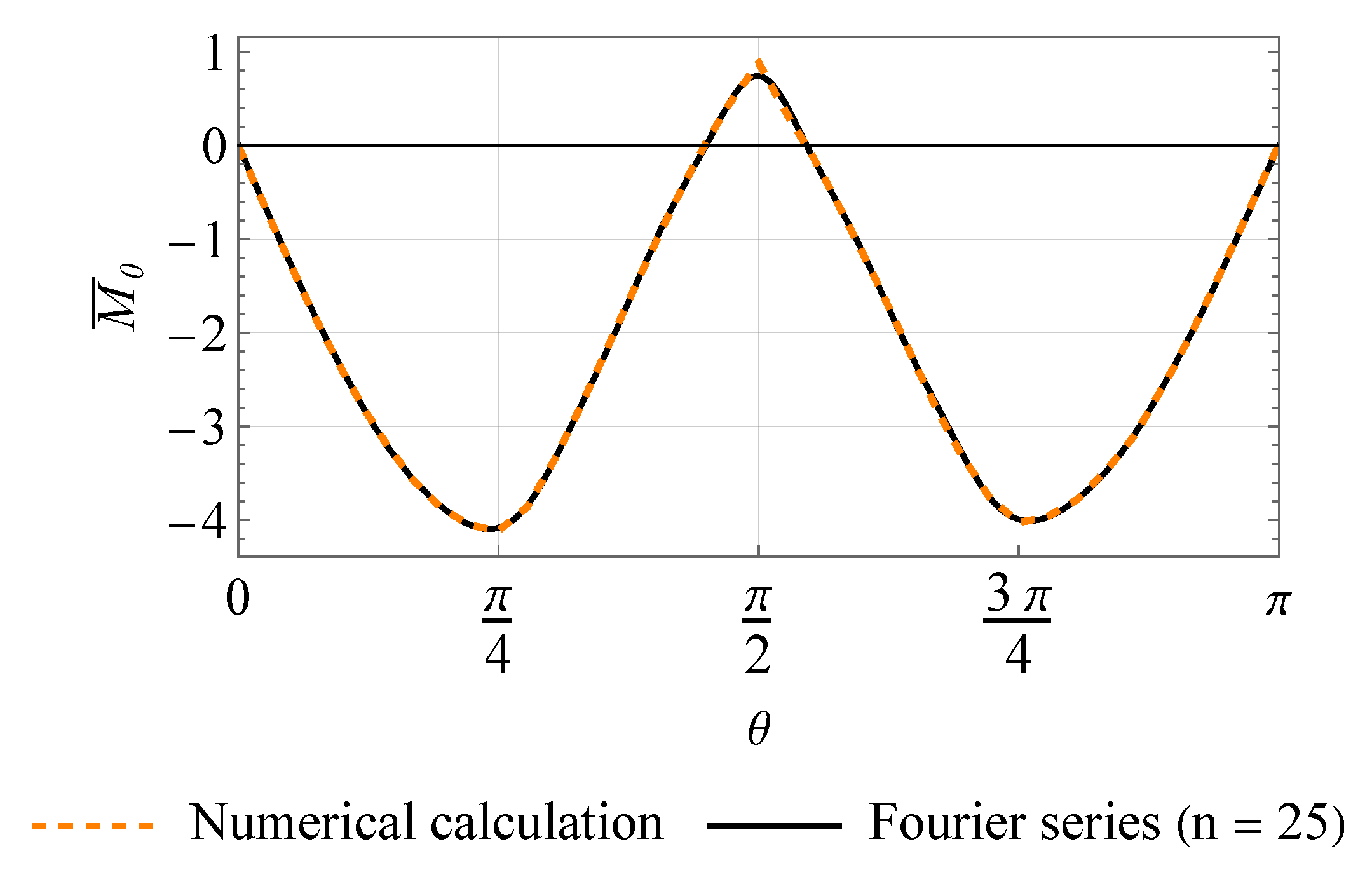
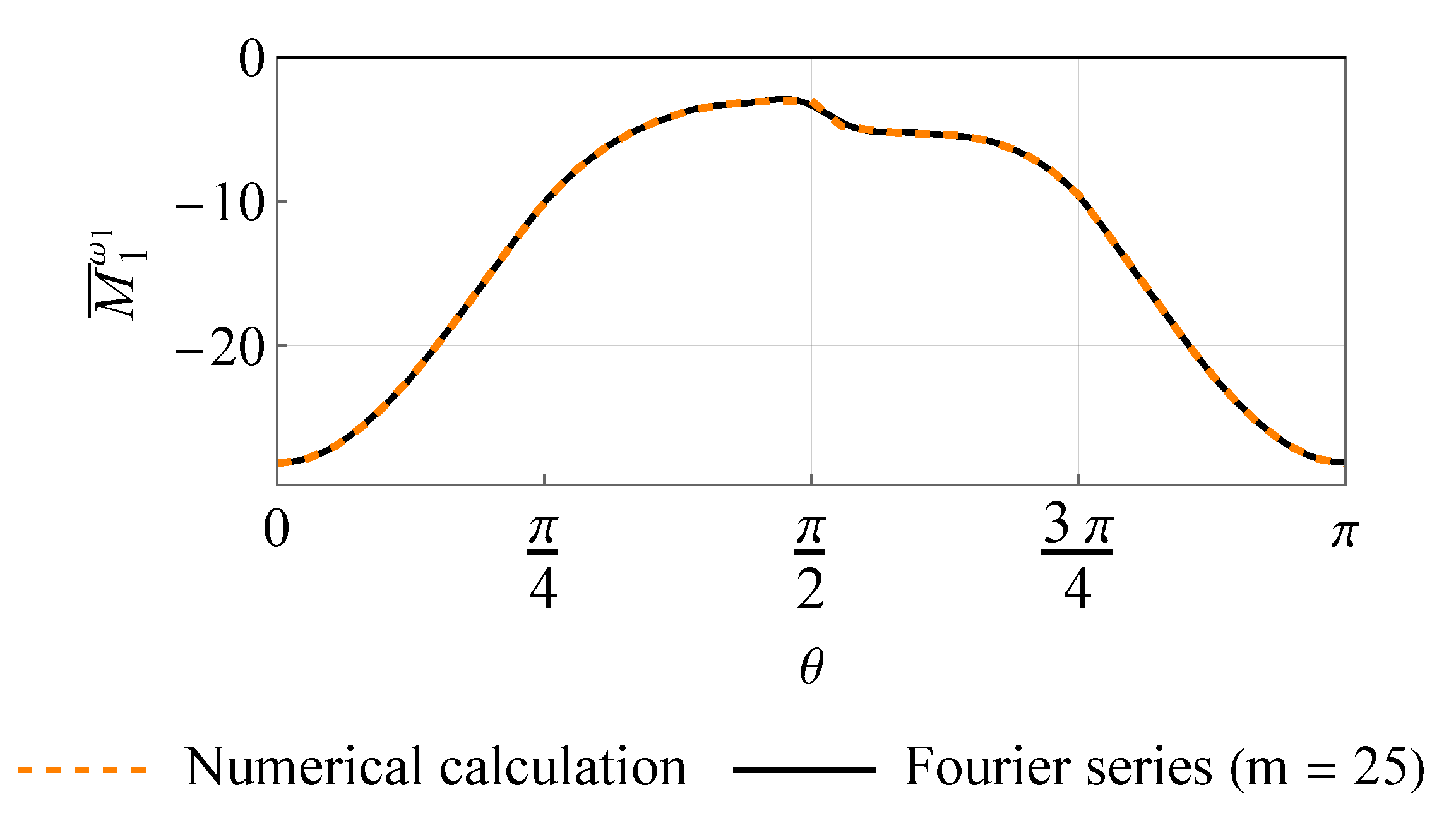
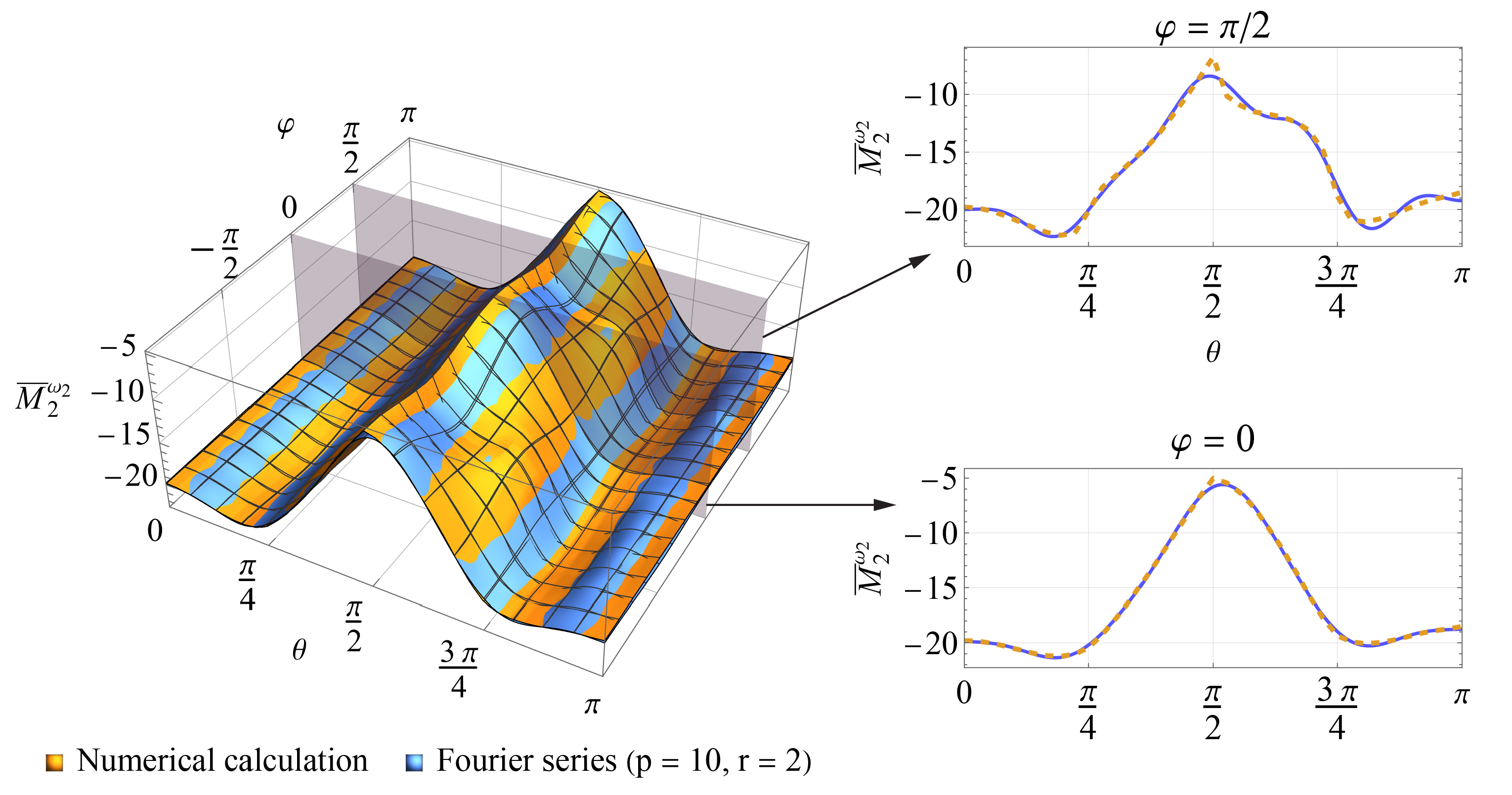
4.1. Aerodynamic Characteristics

The aerodynamic torque coefficients for the example satellite are calculated as follows [30]. Taking into account that, for a body with a reference length of about 1 m, the Knudsen number at altitudes above 130 km is larger than 10, which means that the flow is free molecular, then one can assume that the reflected air molecules’ speed distribution is Maxwellian and calculate the pressure and shear stress coefficients using the Schaaf and Chambre’s approach [41]. The numerical results were approximated by Fourier series according to Equations (21) and (26).

Figure 3 shows the calculated restoring aerodynamic torque coefficient and its Fourier series approximation (Equation (21)). It is worth noting that, in the vicinity of $\theta =\pi /2$, there exists a region where ${\overline{M}}_{\theta }$ is positive. In some cases, this could provoke instability. One of these cases will be studied below. Figure 4 and Figure 5 depict the coefficients ${\overline{M}}_1^{{\omega }_1}$ and ${\overline{M}}_2^{{\omega }_2}$ of the damping torque, respectively, as well as their 2D Fourier series approximation (Equation (26)). The plot for coefficient ${\overline{M}}_3^{{\omega }_3}$ is not shown, since it can easily be obtained by shifting the ${\overline{M}}_2^{{\omega }_2}$ surface by $\pi /2$ along the $\phi$ axis by virtue of the last of Equation (26). It can be seen in Figure 5 that, unlike the spin damping coefficient ${\overline{M}}_1^{{\omega }_1}$, the other two damping torque coefficients slightly vary with $\phi$. It is also interesting that the magnitudes of all damping torque coefficients for the considered shape are substantially higher when the angle of attack is small than when the symmetry axis of the satellite is nearly perpendicular to the flow. One may thus expect more intensive attitude motion damping when the satellite is close to its operational orientation.

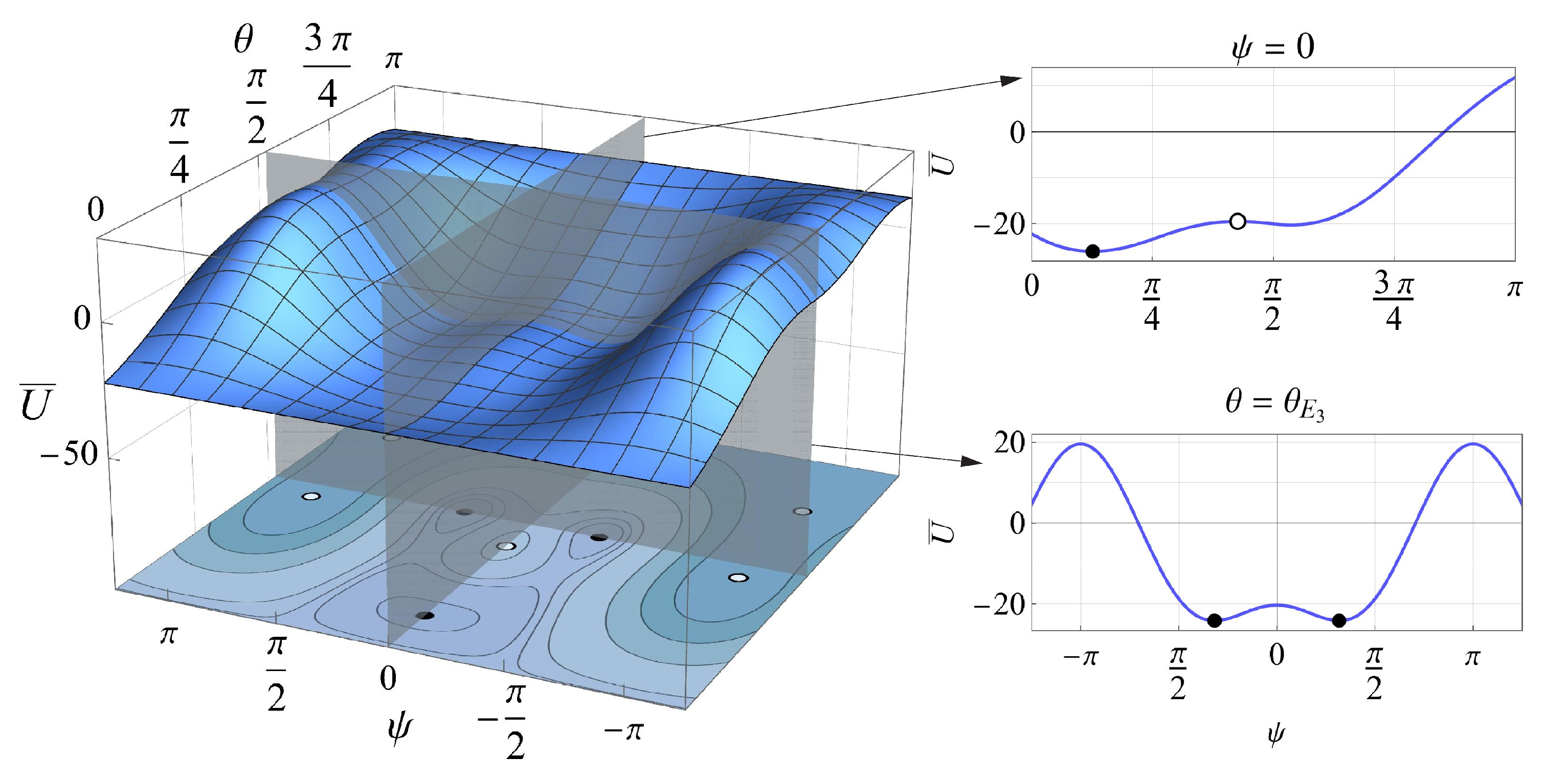
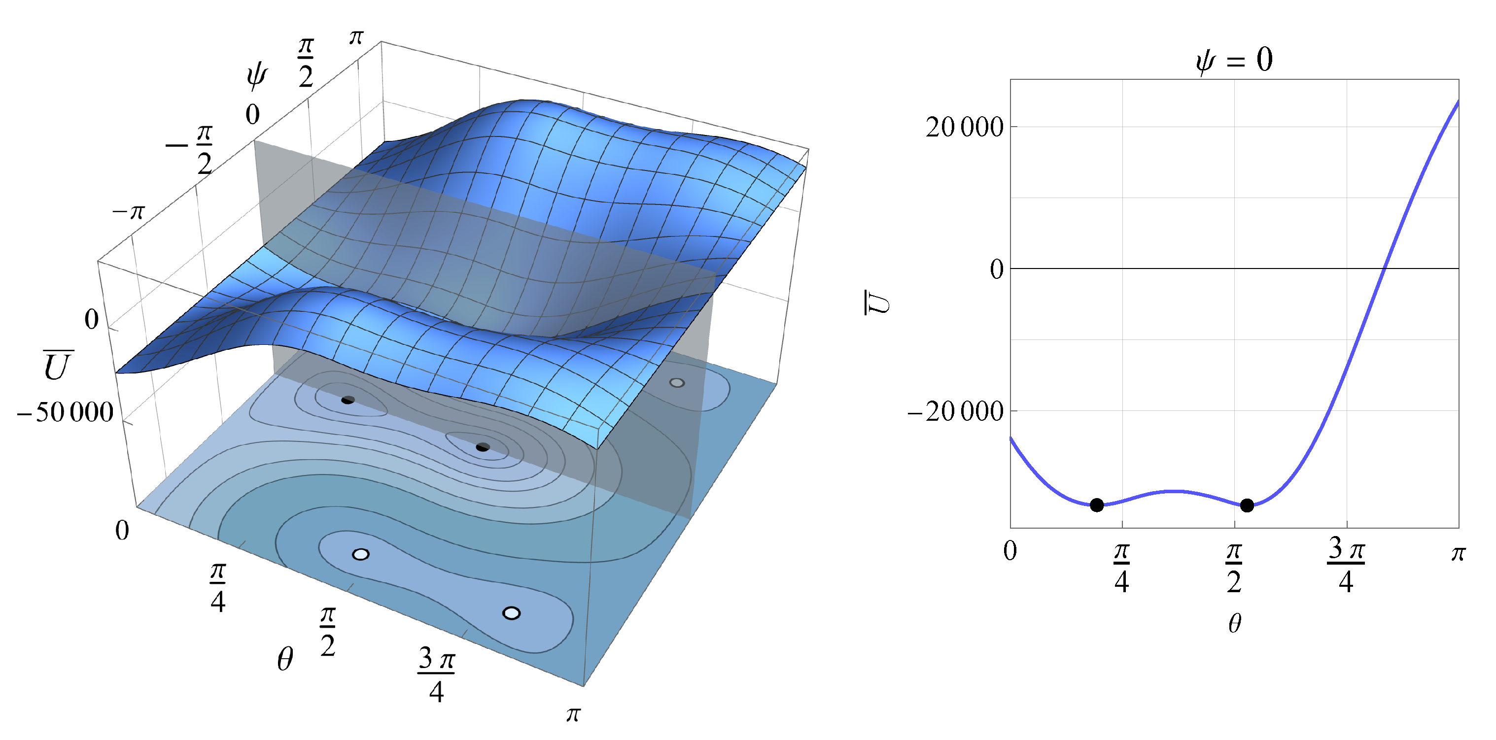
4.2. Dynamic Potential and Equilibrium Positions in Unperturbed Motion

The dimensionless dynamic potential $\overline{U}$ of the unperturbed motion (Equation (43)) is determined by some parameters of the satellite, which were chosen above, namely its shape, the moments of inertia, etc., as well as the initial value of the dimensionless conjugated momentum $\beta$ (Equation (39)) and the orbital altitude. Let us choose two orbital altitudes: 700 km (LEO) and 250 km (VLEO). At 700 km, the gravitational torque and aerodynamic restoring torque have roughly the same order of magnitude. In VLEO, the satellite’s interaction with the atmosphere is much stronger, so the aerodynamic restoring torque is much larger than the gravitational one. The initial conjugated momentum $\beta$ depends on the initial conditions and was chosen arbitrarily, in order to represent the shapes of the dynamic potential, which are typical for the problem under consideration.

Figure 6 and Figure 7 represent the dimensionless dynamic potential for the chosen altitudes as 3D surfaces and the corresponding contour plots. The latter can also be understood as phase portraits of the unperturbed system. The stable and unstable equilibrium positions of the satellite are marked with black and white dots, respectively. Figure 6 shows that, for $h=700$ km and $\beta =33,000$, the equilibrium positions from all three groups (Equations (45)–(47)) are present. The stable positions belong to Groups $E_1$ and $E_3$. In the case of $h=250$ km, $\beta =20$, illustrated by Figure 7, the situation is substantially different: only the positions from Groups $E_1$ and $E_2$ are present, and the stable ones belong to Group $E_1$.

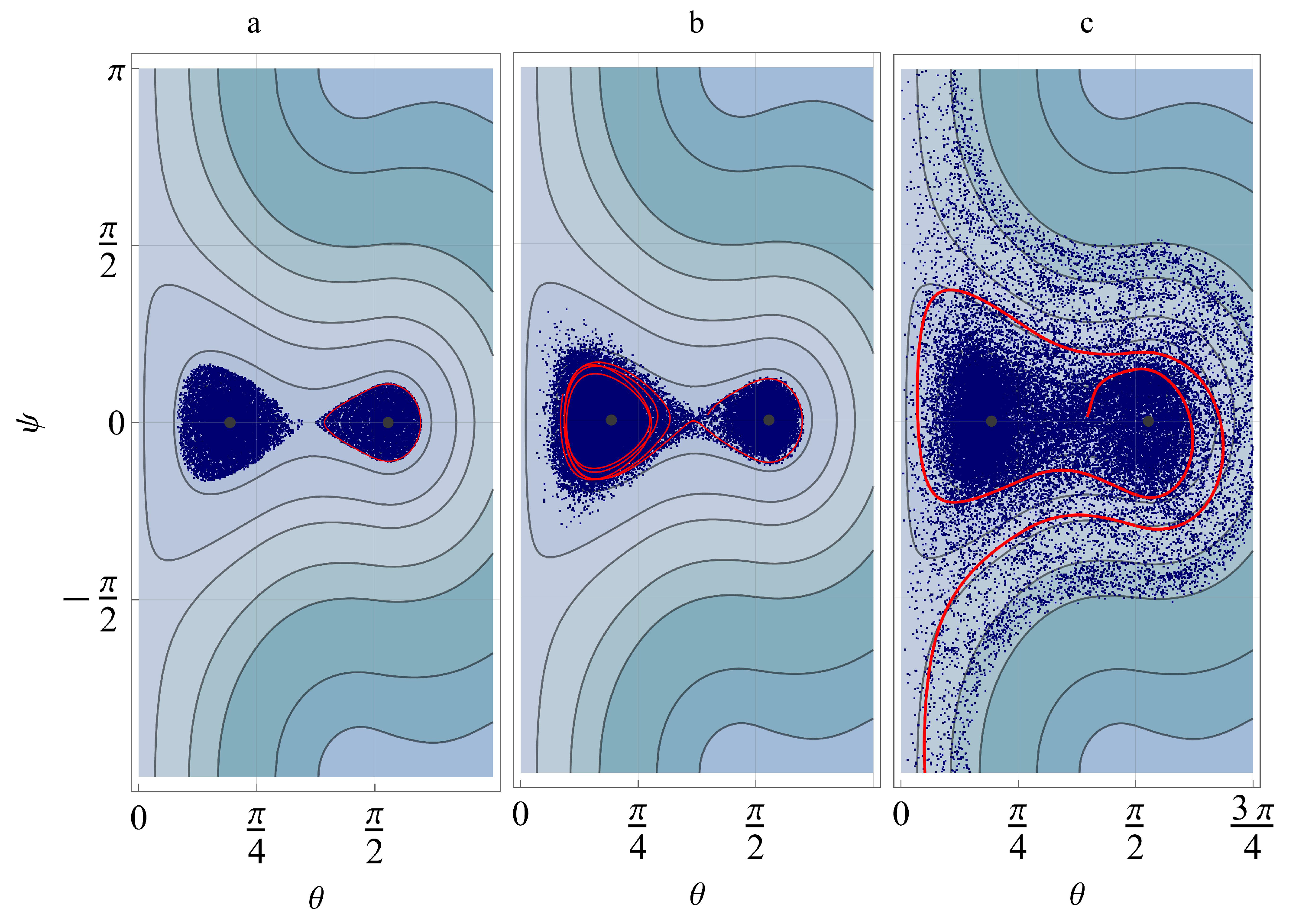
4.3. Simulations of Perturbed Motion

In order to illustrate different possible cases of the attitude motion of the example satellite, the Poincaré surfaces of the section were calculated via the numerical integration of the perturbed equations (Equation (50)) for several phase-space trajectories at two orbital altitudes chosen above. The components of the satellite’s own magnetic moment were taken equal to each other and to unity:

$${\overline{M}}_k=1,$$

(53)

$k=1,2,3$. The initial conditions were chosen in such a way that all trajectories at the same altitude had the same energy (Equation (41)). The simulations were performed for different absolute values of magnetic perturbation, which were determined by the dimensionless parameter $\epsilon$ (Equation (52)). For a better understanding of the influence of each torque acting on the example satellite, the orders of magnitude of the torques are given in

Table 2. Orders of magnitude of the torques acting on the example satellite.

h (km)	Order of Magnitude (N·m)
	Gravitational	Aerodynamic Restoring	Aerodynamic Damping	Magnetic
250	${10}^{-8}$	${10}^{-4}$	${10}^{-12}$	$\epsilon =580$:${10}^{-6}$	$\epsilon =3900$:${10}^{-5}$
700	${10}^{-8}$	${10}^{-7}$	${10}^{-15}$	$\epsilon =0.58$:${10}^{-9}$	$\epsilon =1.35$:${10}^{-8}$

.

Figure 8 and Figure 9 represent the Poincaré surfaces of the section projected onto the $(\theta ,\psi )$ plane, as well as several typical phase trajectories coloured in red. If its own magnetic moment is absent $(\epsilon =0)$, the Poincaré sections are consistent with the phase portrait of the unperturbed system, as shown in Figure 8a and Figure 9a, and all the section points corresponding to the chosen phase trajectories lie in the potential wells, i.e., the satellite oscillates in the vicinity of its stable equilibrium positions. Figure 8b and Figure 9b depict the Poincaré sections for rather weak magnetic perturbations. It can be seen that the system starts to demonstrate chaotic behaviour: the layers connecting different potential wells appear, and the phase trajectories that start in one well may go into another, though the satellite still oscillates near the same set of equilibrium positions, for which $-\pi /2\le \psi \le \pi /2$. In the case of stronger magnetic perturbations, the chaotic behaviour becomes more prominent, and full rotations about the precession axis are possible, as is clearly indicated by Figure 8c and Figure 9c, showing the Poincaré sections with the precession angle $\psi$ distributed in the interval from $-\pi$ to $\pi$.

Thus, the numerical simulations revealed the possibility of chaos in the attitude motion of aerodynamically stabilised spinning deployable satellites in the presence of magnetic perturbations. To cause the chaotic motion in VLEO, where the interaction with the air is stronger and the aerodynamic damping is significant, the magnitude of perturbations needs to be several orders higher than in LEO.

5. Conclusions

The attitude motion of arbitrarily spinning satellites in LEO and VLEO under the action of aerodynamic, gravitational, and magnetic torques was investigated, taking into account the aerodynamic damping. The separation of the equations of motion into the unperturbed and perturbation parts, proposed in the paper, facilitated an intuitive understanding of the satellite’s behaviour and allowed determining several regimes of angular oscillations corresponding to the wells of the dynamic potential surface. The numerical simulations showed that the magnetic perturbations may cause the chaotic attitude motion of the satellite, manifested in the transition between the potential wells. These results revealed the need for active attitude control to prevent chaotic motion in the case of unexpected spin motion, though this is challenging for small satellites due to their power limits. In this regard, another way of eliminating undesirable spin can be proposed, dealing with the design of reliable satellite deployment techniques, reducing the risk of resulting skew aerodynamic shapes.

The future work will focus on related problems not covered in this paper. In particular, it is interesting to control chaos using magnetorquers or movable aerodynamic surfaces in order to transform irregular attitude motions into periodic ones. Another area of research is to investigate the observed effects in a more general case, taking into account the perturbations caused by the evolution of orbital altitude or by the oscillations of flexible elements.

References

1. Nurre, G.S. Effects of aerodynamic torque on an asymmetric, gravity-stabilized satellite. J. Spacecr. Rocket. 1968, 5, 1046–1050. [Google Scholar] [CrossRef]
2. Beletskii, V.; Grushevskii, A. The evolution of the rotational motion of a satellite under the action of a dissipative aerodynamic moment. J. Appl. Math. Mech. 1994, 58, 11–19. [Google Scholar] [CrossRef]
3. Kuznetsova, E.Y.; Sazonov, V.; Chebukov, S.Y. Evolution of the satellite rapid rotation under the action of the gravitational and aerodynamic torques. Mech. Solids 2000, 35, 1–10. [Google Scholar]
4. Maslova, A.; Pirozhenko, A. Modeling of the aerodynamic moment acting upon a satellite. Cosm. Res. 2010, 48, 362–370. [Google Scholar] [CrossRef]
5. DeBra, D.B. The effect of aerodynamic forces on satellite attitude. J. Astronaut. Sci 1959, 6, 40–45. [Google Scholar]
6. Meirovitch, L.; Wallace, F., Jr. On the effect of aerodynamic and gravitational torques on the attitude stability of satellites. AIAA J. 1966, 4, 2196–2202. [Google Scholar] [CrossRef]
7. Beletskii, V.V. Motion of an Artificial Satellite about its Center of Mass; NASA TT F-429; NASA: Washington, DC, USA, 1966.
8. Frik, M.A. Attitude stability of satellites subjected to gravity gradient and aerodynamic torques. AIAA J. 1970, 8, 1780–1785. [Google Scholar] [CrossRef]
9. Pande, K.; Venkatachalam, R. On optimal aerodynamic attitude control of spacecraft. Acta Astronaut. 1979, 6, 1351–1359. [Google Scholar] [CrossRef]
10. Romano, F.; Espinosa-Orozco, J.; Pfeiffer, M.; Herdrich, G.; Crisp, N.; Roberts, P.; Holmes, B.; Edmondson, S.; Haigh, S.; Livadiotti, S.; et al. Intake design for an Atmosphere-Breathing Electric Propulsion System (ABEP). Acta Astronaut. 2021, 187, 225–235. [Google Scholar] [CrossRef]
11. Vaidya, S.; Traub, C.; Romano, F.; Herdrich, G.; Chan, Y.A.; Fasoulas, S.; Roberts, P.; Crisp, N.; Edmondson, S.; Haigh, S.; et al. Development and analysis of novel mission scenarios based on Atmosphere-Breathing Electric Propulsion (ABEP). CEAS Space J. 2022, 14, 689–706. [Google Scholar] [CrossRef]
12. Aslanov, V.; Sizov, D. 3U CubeSat aerodynamic design aimed to increase attitude stability and orbital lifetime. In Proceedings of the International Astronautical Congress, IAC, Naples, Italy, 12–14 October 2020. [Google Scholar]
13. Otsu, H. Aerodynamic Characteristics of Re-Entry Capsules with Hyperbolic Contours. Aerospace 2021, 8, 287. [Google Scholar] [CrossRef]
14. Jiang, Y.; Zhang, J.; Tian, P.; Liang, T.; Li, Z.; Wen, D. Aerodynamic drag analysis and reduction strategy for satellites in Very Low Earth Orbit. Aerosp. Sci. Technol. 2022, 132, 108077. [Google Scholar] [CrossRef]
15. Ivanov, D.; Monakhova, U.; Guerman, A.; Ovchinnikov, M. Decentralized Control of Nanosatellite Tetrahedral Formation Flying Using Aerodynamic Forces. Aerospace 2021, 8, 199. [Google Scholar] [CrossRef]
16. Traub, C.; Fasoulas, S.; Herdrich, G.H. A planning tool for optimal three-dimensional formation flight maneuvers of satellites in VLEO using aerodynamic lift and drag via yaw angle deviations. Acta Astronaut. 2022, 198, 135–151. [Google Scholar] [CrossRef]
17. Miyamoto, K.; Chujo, T.; Watanabe, K.; Matunaga, S. Attitude dynamics of satellites with variable shape mechanisms using atmospheric drag torque and gravity gradient torque. Acta Astronaut. 2023, 202, 625–636. [Google Scholar] [CrossRef]
18. Yamada, K.; Nagata, Y.; Abe, T.; Suzuki, K.; Imamura, O.; Akita, D. Suborbital reentry demonstration of inflatable flare-type thin-membrane aeroshell using a sounding rocket. J. Spacecr. Rocket. 2015, 52, 275–284. [Google Scholar] [CrossRef]
19. Berthet, M.; Yamada, K.; Nagata, Y.; Suzuki, K. Feasibility assessment of passive stabilisation for a nanosatellite with aeroshell deployed by orbit-attitude-aerodynamics simulation platform. Acta Astronaut. 2020, 173, 266–278. [Google Scholar] [CrossRef]
20. Alpert, H.; Miller, R.; Kazemba, C.; Swanson, G.; Cheatwood, F. LOFTID Heat Flux Gauge Calibration: What is Truth? In Proceedings of the International Planetary Probe Workshop, Hamelin, Germany, 19–23 April 2021. [Google Scholar]
21. Zuppardi, G.; Savino, R.; Mongelluzzo, G. Aero-thermo-dynamic analysis of a low ballistic coefficient deployable capsule in Earth re-entry. Acta Astronaut. 2016, 127, 593–602. [Google Scholar] [CrossRef] [Green Version]
22. Carná, S.R.; Bevilacqua, R. High fidelity model for the atmospheric re-entry of CubeSats equipped with the drag de-orbit device. Acta Astronaut. 2019, 156, 134–156. [Google Scholar] [CrossRef]
23. Balaraman, P.; Stephen Joseph Raj, V.; Sreehari, V.M. Static and Dynamic Analysis of Re-Entry Vehicle Nose Structures Made of Different Functionally Graded Materials. Aerospace 2022, 9, 812. [Google Scholar] [CrossRef]
24. Iñarrea, M.; Lanchares, V. Chaotic pitch motion of an asymmetric non-rigid spacecraft with viscous drag in circular orbit. Int. J. Non-Linear Mech. 2006, 41, 86–100. [Google Scholar] [CrossRef]
25. Akulenko, L.; Leshchenko, D.; Rachinskaya, A. Evolution of the satellite fast rotation due to the gravitational torque in a dragging medium. Mech. Solids 2008, 43, 173–184. [Google Scholar] [CrossRef]
26. Leshchenko, D.; Ershkov, S.; Kozachenko, T. Evolution of a heavy rigid body rotation under the action of unsteady restoring and perturbation torques. Nonlinear Dyn. 2021, 103, 1517–1528. [Google Scholar] [CrossRef]
27. Yue, B.Z. Study on the chaotic dynamics in attitude maneuver of liquid-filled flexible spacecraft. AIAA J. 2011, 49, 2090–2099. [Google Scholar] [CrossRef]
28. Chegini, M.; Sadati, H.; Salarieh, H. Chaos analysis in attitude dynamics of a flexible satellite. Nonlinear Dyn. 2018, 93, 1421–1438. [Google Scholar] [CrossRef]
29. Aslanov, V.S. Chaotic attitude dynamics of a LEO satellite with flexible panels. Acta Astronaut. 2021, 180, 538–544. [Google Scholar] [CrossRef]
30. Aslanov, V.S.; Sizov, D.A. Chaos in flexible CubeSat attitude motion due to aerodynamic instability. Acta Astronaut. 2021, 189, 310–320. [Google Scholar] [CrossRef]
31. Iñarrea, M. Chaos and its control in the pitch motion of an asymmetric magnetic spacecraft in polar elliptic orbit. Chaos Solitons Fractals 2009, 40, 1637–1652. [Google Scholar] [CrossRef]
32. Liu, Y.; Chen, L. Chaos in Spatial Attitude Motion of Spacecraft. In Chaos in Attitude Dynamics of Spacecraft; Springer: Berlin/Heidelberg, Germany, 2013; pp. 99–129. [Google Scholar]
33. Aslanov, V.S.; Sizov, D.A. Chaotic pitch motion of an aerodynamically stabilized magnetic satellite in polar orbits. Chaos Solitons Fractals 2022, 164, 112718. [Google Scholar] [CrossRef]
34. ISO 14222:2013; International Standard. Space Environment (Natural and Artificial)—Earth Upper Atmosphere. International Organization for Standardization: Geneva, Switzerland, 2013.
35. Schaub, H.; Junkins, J.L. Analytical Mechanics of Space Systems; AIAA: Reston, VA, USA, 2009. [Google Scholar]
36. Aslanov, V.S. Rigid Body Dynamics for Space Applications; Butterworth-Heinemann: Oxford, UK, 2017. [Google Scholar]
37. Shrivastava, S.; Modi, V. Satellite attitude dynamics and control in the presence of environmental torques-A brief survey. J. Guid. Control. Dyn. 1983, 6, 461–471. [Google Scholar] [CrossRef]
38. Gallais, P. Atmospheric Re-Entry Vehicle Mechanics; Springer Science & Business Media: Berlin/Heidelberg, Germany, 2007. [Google Scholar]
39. Chernousko, F.L.; Akulenko, L.D.; Leshchenko, D.D. Evolution of Motions of a Rigid Body about Its Center of Mass; Springer: Berlin/Heidelberg, Germany, 2017. [Google Scholar]
40. Leshchenko, D.; Ershkov, S.; Kozachenko, T. Rotations of a Rigid Body Close to the Lagrange Case under the Action of Nonstationary Perturbation Torque. J. Appl. Comput. Mech. 2022, 8, 1023–1031. [Google Scholar]
41. Schaaf, S.; Chambre, P. Flow of Rarefied Gases, High Speed Aerodynamics and Jet Propulsion. In Fundamentals of Gas Dynamics; Princeton University Press: Princeton, NJ, USA, 1958; Volume 3. [Google Scholar]
Figure 1. Coordinate frames and Euler angles.
Aerospace 10 00192 g001
Figure 2. Example satellite.
Aerospace 10 00192 g002
Figure 3. Restoring aerodynamic torque coefficient.
Aerospace 10 00192 g003
Figure 4. Coefficient M ¯ 1 ω 1 of the damping torque.
Aerospace 10 00192 g004
Figure 5. Coefficient M ¯ 2 ω 2 of the damping torque.
Aerospace 10 00192 g005
Figure 6. Dimensionless dynamic potential in LEO ( h = 700 km, β = 33 , 000 ). Black dots: stable equilibrium; white dots: unstable equilibrium.
Aerospace 10 00192 g006
Figure 7. Dimensionless dynamic potential in VLEO ( h = 250 km, β = 20 ). Black dots: stable equilibrium; white dots: unstable equilibrium.
Aerospace 10 00192 g007
Figure 8. Poincaré sections ( h = 250 km, β = 33,000 ); (a): ε = 0 , (b): ε = 580 , (c): ε = 3900 . Red lines: typical phase trajectories.
Aerospace 10 00192 g008
Figure 9. Poincaré sections ( h = 700 km, β = 20 ); (a): ε = 0 , (b): ε = 0.58 , (c): ε = 1.35 . Red lines: typical phase trajectories.
Aerospace 10 00192 g009