Evaluating Airfoil Mesh Quality with Transformer

Abstract

Mesh quality is a major factor affecting the structure of computational fluid dynamics (CFD) calculations. Traditional mesh quality evaluation is based on the geometric factors of the mesh cells and does not effectively take into account the defects caused by the integrity of the mesh. Ensuring the generated meshes are of sufficient quality for numerical simulation requires considerable intervention by CFD professionals. In this paper, a Transformer-based network for automatic mesh quality evaluation (Gridformer), which translates the mesh quality evaluation into an image classification problem, is proposed. By comparing different mesh features, we selected the three features that highly influence mesh quality, providing reliability and interpretability for feature extraction work. To validate the effectiveness of Gridformer, we conduct experiments on the NACA-Market dataset. The experimental results demonstrate that Gridformer can automatically identify mesh integrity quality defects and has advantages in computational efficiency and prediction accuracy compared to widely used neural networks. Furthermore, a complete workflow for automatic generation of high-quality meshes based on Gridformer was established to facilitate automated mesh generation. This workflow can produce a high-quality mesh with a low-quality mesh input through automatic evaluation and optimization cycles. The preliminary implementation of automated mesh generation proves the versatility of Gridformer.

1. Introduction

Computational fluid dynamics (CFD) has been continuously expanded from the initial field of aerospace to [1] architectural design [2], energy engineering [3], automotive engineering [4], food engineering [5], and the agricultural environment [6]. The complete CFD process is divided into three steps [7]: (1) the generation of the mesh; (2) the determination of the CFD control equations for the solution, and the numerical calculation method; and (3) the calculation and visualization of some parameters such as the velocity field, pressure field, and temperature field. Throughout the process, the work on mesh quality evaluation in the first step proved to determine the accuracy of the numerical simulations for the subsequent work [8]. Numerical simulations have proven critical for the design and manufacture of aircraft [9], so mesh quality evaluation is a very important part of the process. The shape of the mesh was found to have a significant effect in identifying the quality of the mesh in later studies. Many metrics were introduced to be added to the mesh quality evaluation criteria [10]. For example, length ratio, skew, shape, volume, Jacobian matrix, and other quality criteria. However, these quality criteria are flawed in that they only examine the geometry of individual mesh elements, ignoring the impact of the wholeness between meshes on the evaluation of mesh quality. Knupp [11] studied the relationship between the mesh quality metric, the truncation error, and the interpolation error. The results show that certain metrics are not related to the accuracy of the final calculation. They are mainly used to detect meshes with defects and to guide the generation and optimization of meshes. The above quality indicators only represent local features and not global features. To evaluate the overall quality of the mesh, CFD professionals with experience are required to frequently check and evaluate the current mesh quality and make timely adjustments. The whole process takes much time, resulting in high computational costs and low efficiency, which seriously hinder the development of automatic mesh generation technology.

Automated mesh generation is at the forefront of research in the field of mesh generation technology and has already achieved technological breakthroughs in certain areas. Hetmaniuk and Knupp [12] improved the mesh optimization algorithm for two-dimensional triangular surface meshes by swapping the edges and moving the nodes to optimize the objective function, reducing the error in the difference calculation. The unstructured appendage layer T-Rex algorithm was introduced by PointWise [13]; it is based on the cell fusion mesh processing technique to further optimize the mesh of the unstructured appendage layer, which brings powerful technical support for automatic mesh generation. These studies have largely solved the problem of automating mesh generation for CFD attachment layers, such as automatic control of mesh cell quality, optimization of the mesh, and reduction of errors in the calculation. Solving the above complex engineering problems has laid a good technical foundation for the fully automatic generation of high-quality meshes.

In addition to traditional goal-oriented optimization algorithms for mesh cells, machine learning methods have also been used to guide the generation of high-quality meshes. Keefe Huang et al. [14] presented a convolutional neural network trained based on massive data points to predict the optimal density of the mesh. Data for arbitrarily shaped 2D channels/mesh of wind-tunnel-like flow. The results of the network predictions are fed into any mesh generation and CFD partitioning tool to guide the generation of optimal density meshes, further promoting automated mesh generation. However, the process requires manual involvement for quality evaluation and cannot be applied to other meshes with poor-quality properties. For automated mesh generation, the biggest challenge remains the reliance on manual mesh quality evaluation.

With the breakthrough of deep-learning algorithms of neural networks and the rapid development of artificial intelligence in recent years, successful applications have been made to many labor-intensive problems constrained by a priori knowledge [15,16]. Complex features are constructed by discovering the relationship between inputs and outputs through simple neural network functions. The parameters of the model are finally optimized interactively by a gradient descent algorithm to autonomously discover the high-dimensional meaning behind the data. Deep learning is currently used in various fields, including computer vision, natural language processing, and reinforcement learning. The Transformer [17], which has been available since 2017, is designed for sequence modeling and transduction tasks. It is known for modeling long-term dependencies in data through attention mechanisms and is mostly used in the field of natural language processing (NLP). Starting in 2020, Transformer-type networks have been used in the CV field [18], achieving amazing results in image classification in particular. Although deep learning is used in many fields, it is rarely used in the field of quality assessment.

In the relevant research field, such as point cloud quality assessment (PCQA) and image quality assessment, some state-of-the-art techniques have shown promising results. Liu et al. [19] proposed a no-reference metric based on the sparse convolutional neural network ResSCNN for point cloud quality evaluation, which can achieve a high level of accuracy. Zhou et al. [20] proposed a generic, no-reference, objective point cloud quality metric based on Structure Guided Resampling (SGR) to automatically evaluate the visual quality of 3D point clouds. According to the combined effect of 3D geometric features and related attributes, geometric density features, color naturalness features, and angular consistency features are used to predict the perceived quality of distorted 3D point clouds. Lu et al. [21] created a Reinforced Transformer Network (RTN) by using Transformer’s MIL module in combination with their proposed Progressive Reinforcement learning-based Instance Discarding module. It is used for image quality evaluation to determine the local areas of final quality. You and Korhonen [22] proposed the use of a shallow Transformer encoder on top of a feature map extracted by convolutional neural networks for evaluating images of arbitrary resolution. These relevant studies provide insights in our study for solving the problem of mesh quality evaluation.

In the procedure of mesh quality evaluation, Zhang et al. [23] proposed three basic requirements for mesh quality: orthogonality, smoothness, and spacing distribution properties.

• Orthogonality means that the lines (faces) of the mesh are as orthogonal as possible.
• Smoothness means that the transition of the mesh in physical space should be slow and smooth, rather than abrupt and steep, otherwise rapid changes in the volume of the neighboring cells could lead to truncation errors.
• Spacing distribution characteristic refers to the fact that the continuous region is discretized so that the characteristic solutions of the flow (shear layer, separation region, surge, boundary layer, and mixing region) are directly related to the density and distribution of the nodes on the mesh.

Transformer that features Multi-Head Self-Attention (MSA), position encoding, and slide windows can learn the geometric properties of the mesh cells and establish global associations of all the meshes. Based on these characteristics, Transformer can identify the orthogonality of the mesh cells and also recognize the smoothness and spacing distribution characteristics between the integral meshes.

In summary, the traditional quality criteria based on the geometry of the mesh cells only check the quality of individual elements, represent only local features of the mesh, and require manual involvement, which is inefficient. According to Transformer’s efficient learning ability, an approach specifically suitable for mesh quality evaluation, i.e., Gridformer, is designed in this paper. Gridformer can be used to learn the properties of mesh quality. In contrast, evaluating mesh quality through Transformer takes into account not only the local features of the mesh but also defects caused by the integrity of the mesh. Most importantly, the method reduces the need for manual involvement, greatly improving the efficiency of high-quality mesh generation and laying the foundation for automated mesh generation. The NACA-Market [24] dataset is cited to demonstrate the validity of the Gridformer-based mesh quality evaluation method. Based on experiments that are compared with other commonly used neural networks on GPUs, the Gridformer achieves the highest accuracy and the lowest parameter overhead on the NACA-Market dataset. To better validate the practicality and robustness of Gridformer, a high-quality mesh generation workflow based on Gridformer was established. Experiments show that when Gridformer is combined with a mesh optimization algorithm, the initial poor quality of the mesh can be automatically improved during the workflow. The whole process requires almost no manual involvement.

2. Related Work

2.1. Traditional Mesh Quality Evaluation Criteria

CFD meshes can be divided into three types of computational meshes: structural, non-structural, and hybrid meshes. Directly defining a function to take the integral mesh input for evaluation is relatively difficult, usually using the quality criteria of the mesh cell. For two-dimensional mesh cells, there are only two metrics to focus on, shape and size. The two metrics can be combined to form a shape–size metric to detect distorted meshes. The two-dimensional meshes are mainly triangles and quadrilaterals, with quality metrics such as cell length, cell edge length ratio, internal angle size, and warp angle [25]. For 2D triangles, the main checks are cell length, aspect ratio, and twist angle. The aspect ratio metric on two-dimensional triangles [26] is as follows:

$$AR=\frac{L_{\max \left(L_0,L_1,L_2\right)}}{4\sqrt{3}S}$$

(1)

In Equation (1), $L_{max}$ is the longest side of the triangle length. $L_0,L_1,L_2$ are the length of the three sides of the triangle, and $S$ is the area of the triangle.

For 2D quadrilateral mesh metrics, including cell length, warp, aspect ratio, Jacobi ratio, and chord deviation. The two-dimensional quadrilateral aspect ratio metrics [26] are as follows:

$$AR=\max \left(\frac{\left|e_x\right|}{\left|e_y\right|},\frac{\left|e_y\right|}{\left|e_x\right|}\right),$$

(2)

where

$$\begin{gathered} e_x=\frac{1}{2}\left[\left(x_1-x_0\right)+\left(x_2-x_3\right)\right], \\ {e}_y=\frac{1}{2}\left[\left(x_3-x_0\right)+\left(x_2-x_1\right)\right] \end{gathered}$$

In Equation (2), $x_0$, $x_1$, $x_2$, and $x_3$ are the horizontal coordinates of the four points of the quadrilateral. The $AR$ takes values from 1.0 to ∞. When the mesh of cells is a square or diamond ($AR$ = 1), the mesh quality is best.

Skewness [27], as a metric of mesh distortion, is an angle measure that the mesh cell has relative to the angle of the ideal cell type. It determines how close a face or cell is to the ideal (equilateral or equiangular). It is calculated as follows:

$$\mathrm{skewness}=\max \left[\frac{{\theta }_{max}-{\theta }_e}{180-{\theta }_e},\frac{{\theta }_e-{\theta }_{min}}{{\theta }_e}\right]$$

(3)

In Equation (3), ${\theta }_{max}$ is the maximum internal angle of the unit or face. ${\theta }_{min}$ is the minimum internal angle of the unit or face. ${\theta }_e$ is the angle of the ideally shaped unit or face.

CAE software such as ICEM CFD [28] and PointWise [29] have suggested parametric modules for ensuring mesh quality delineation. For example, element quality is used not only to evaluate two-dimensional mesh cells but also extends to three-dimensional mesh cells. The definitions are as follows:

$${\mathit{Quality}}_{2D}=C\left(\frac{\mathit{area}}{\sum {\left({\mathit{EdgeLength}}_{2D}\right)}^2}\right)$$

(4)

$${\mathit{Quality}}_{3D}=C\left(\frac{\mathit{volume}}{\sqrt{\sum {\left({\mathit{EdgeLength}}_{3D}^2\right)}^3}}\right)$$

(5)

In Equations (4) and (5), $C$ is a constant that takes values according to the cell type. The area is the area of the 2D mesh cell. The volume is the volume of the 3D mesh cell. EdgeLength is the edge length of the mesh cell. In general, the mesh quality is best when Quality = 1. The mesh quality is worst when Quality = 0.

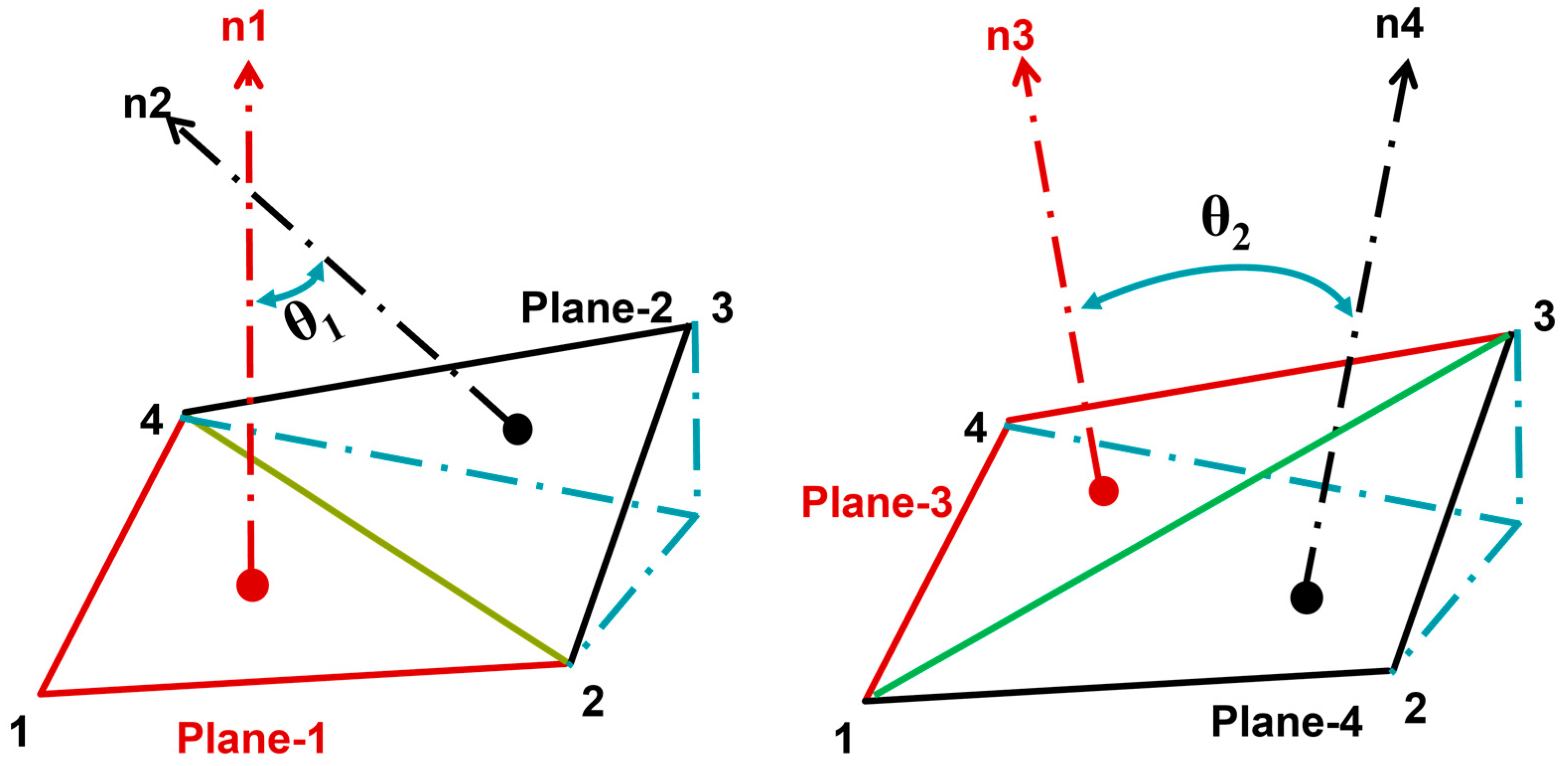
The ICEM CFD also offers a standard called warpage angle, which is defined as the angle between the normals of two (triangular) planes formed by dividing the quadrilateral elements along the diagonal. As shown in Figure 1 below, the largest of the two angles is the warpage angle with an ideal value = 0° (<5° to 10° is acceptable). The calculation is defined as follows:

2.2. Recent Advances in Mesh Quality Evaluation

In addition to traditional mesh quality criteria based on mesh cells, machine learning methods have also been used. For example, feature engineering is used to construct inputs to evaluate the mesh quality. The main method used in this category is the support vector machine [30], which is a linear model for solving classification and regression problems. Yildiz et al. [31] presented a support vector regression model to evaluate the mesh quality of 3D shapes. Specifically, the quality metric is specified by a priori knowledge about the geometric properties of the mesh cells, which is then fed into a support vector regression model to predict the quality. Sprave and Drescher [32] evaluated mesh quality using a data-driven approach. The work uses off-the-shelf machine-learning techniques, including random forests and feed-forward neural networks. However, these features rely on a priori knowledge extraction, do not compare the effects of different features on prediction results, and lack interpretability and reliability.

With the booming growth of data and upgrades in hardware such as GPUs, deep learning has been able to solve many labor-intensive problems. Neural networks can automatically extract potential high-level features from raw data through convolution and pooling, which is applied to computer vision tasks, such as image classification [33], target detection [34], and segmentation [35]. GridNet [24] is a CNN-based mesh quality evaluation model developed through the properties between 2D meshes and mesh data. First, the geometric attributes of the mesh elements are extracted using a priori knowledge as the input features of the model. Then, experiments with structured meshes are conducted to demonstrate the feasibility of neural networks for mesh quality evaluation. However, for feature extraction based only on a priori knowledge and without comparison with other mesh features, there is a lack of interpretability and reliability. The CNN-based GridNet model requires stacking the number of network layers to take into account the overall correlation between the data. As the number of network layers increases, the calculation amount increases, and the performance decreases.

Transformer is already very mature in the field of NLP and later proved its powerful expression and learning capabilities in engineering fields, including CV. Excellent results have been achieved in the areas of image classification [36], image enhancement [37], image generation [38], and pose estimation [39]. The structure of Transformer is shown in Figure 2 [17]. Using the full attention structure, the traditional encoder–decoder model, combined with the inherent model of CNN [40], is abandoned, and a broader receptive field is obtained. Firstly, Transformer has CNN’s ability to learn features automatically and efficiently from multilayer nonlinear transformations. Secondly, positional encoding through self-attention obtains the link between the data and data positions relationship. Finally, the information learned from different head parts is combined in the multi-head attention mechanism to increase computational efficiency. Based on these features, Transformer has a broader receptive field than CNN, focusing more on the connection of the local mesh and the quality of the integral mesh. It can identify the smoothness, orthogonality, and reasonable mesh spacing distribution more accurately and efficiently. During the mesh generation process, Transformer automatically learns data features through nonlinear transformations in multiple modules, eliminating the need for meshing engineers to manually design their features. Although Transformer is widely used in the image field, little research has been done on mesh quality evaluation.

In summary, the traditional mesh quality criteria do not pay much attention to the quality attributes such as smoothness and spacing distribution of the mesh as a whole. The CNN-based GridNet does not learn the positional relationship between meshes during the evaluation of mesh quality. Since the receptive field is not large enough, the feature learning between the entire mesh is not precise enough. More importantly, a certain amount of interpretability is not provided. In this paper, we design a Gridformer model applied to mesh quality evaluation. The best features are selected according to the influence of different features on the prediction results, providing interpretability and reliability for mesh quality evaluation. Experiments have shown that Gridformer accurately identifies mesh quality defect classes with minimal computational overhead and facilitates automated mesh generation.

3. Method

In this paper, mesh quality evaluation is defined as an image classification task. Image classification is an image processing method that distinguishes different classes of targets based on their respective different features reflected in the image information. In this study, the input mesh is regarded as an image, and the eight quality attributes of the mesh are considered as eight classes. A supervised learning approach is used to evaluate mesh quality, converting the mesh file to an image data input format recognized by the Gridformer model through a mesh pre-processing algorithm. After training, the mesh quality is predicted based on pre-defined classes.

3.1. Mesh Pre-Processing Algorithm

An airfoil mesh consists of a set of group point coordinates or mesh elements, but the Transformer requires the input in image data format. How to quantize mesh samples is a problem to be solved. The existing one-hot coding, Bayesian target coding, and other data representation methods may not represent the characteristics of the mesh.

The geometric properties of the mesh elements are used to extract the mesh features to simulate the three-channel input of the picture. This method converts the mesh data into the input matrix needed for training in three steps. 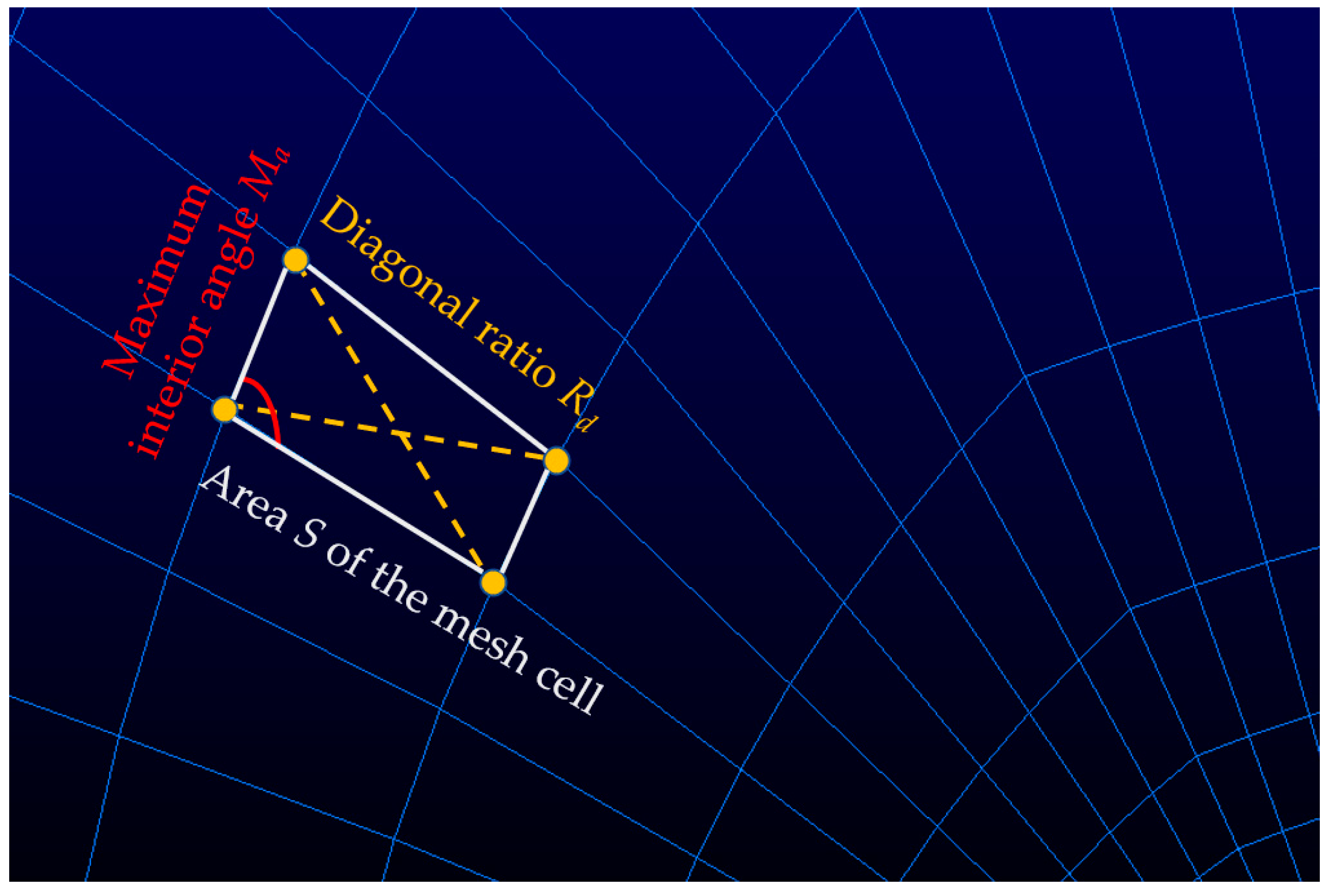In the first step, according to the geometric properties of the mesh, the length L_x, the length L_y, the length D_x of the diagonal, the length D_y of the diagonal, the diagonal ratio R_d, the ratio R_ls of the longest side to the shortest side, area S of the mesh cell, and the maximum interior angle M_a are extracted. In the second step, three properties are selected from the above to compose a three-channel matrix input to Gridformer for comparison experiments. For an intuitive understanding of the features selected in the first step, some features (the diagonal ratio R_d, area S of the mesh cell, maximum interior angle M_a) are showed in Figure 3. The first row corresponds to the features of the outermost elements of the airfoil mesh, and the last row corresponds to the features of the elements of the boundary layer of the airfoil mesh.

The comparative experiments on extracting the best mesh features in the third step provide interpretability and reliability for mesh quality evaluation to some extent. Since Gridformer has global modeling capabilities and possesses relative position encoding, it can efficiently obtain key information such as mesh smoothness and spacing distribution.

In the three-channel input matrix extracted, the difference in values between the three channels is too large. For example, the ratio value of the longest edge to the shortest edge is too far from the mesh cell area and the maximum interior angle of the mesh. Such an irregular data distribution tends to cause the loss descent curve to be more zigzag during the training process, which leads to a slow convergence rate. The normalization method allows the data to be mapped within a certain range, decreasing the effects caused by differences in values between the data. To enable accelerated convergence and enhance the model robustness, we applied Z-score normalization to the input matrix before training, which is defined as follows:

$$\mathrm{Z}=\frac{x-\overline{x}}{\mathsf{\sigma }}$$

(6)

In Equation (6), $\overline{x}$, $\mathsf{\sigma }$ are the mean and standard deviation of the original data $x$. By this normalization, the data values are normally distributed at a mean of 0 and a standard value of 1. Experiments show that prediction accuracy can be improved by normalization.

3.2. Network Structure

For learning large amounts of mesh data, the design of the network requires accuracy. During the mesh generation process, the results of the quality evaluation need to be fed back in time for tuning, so efficiency also needs to be ensured. Designing models that have a good balance between high accuracy and efficiency is challenging.

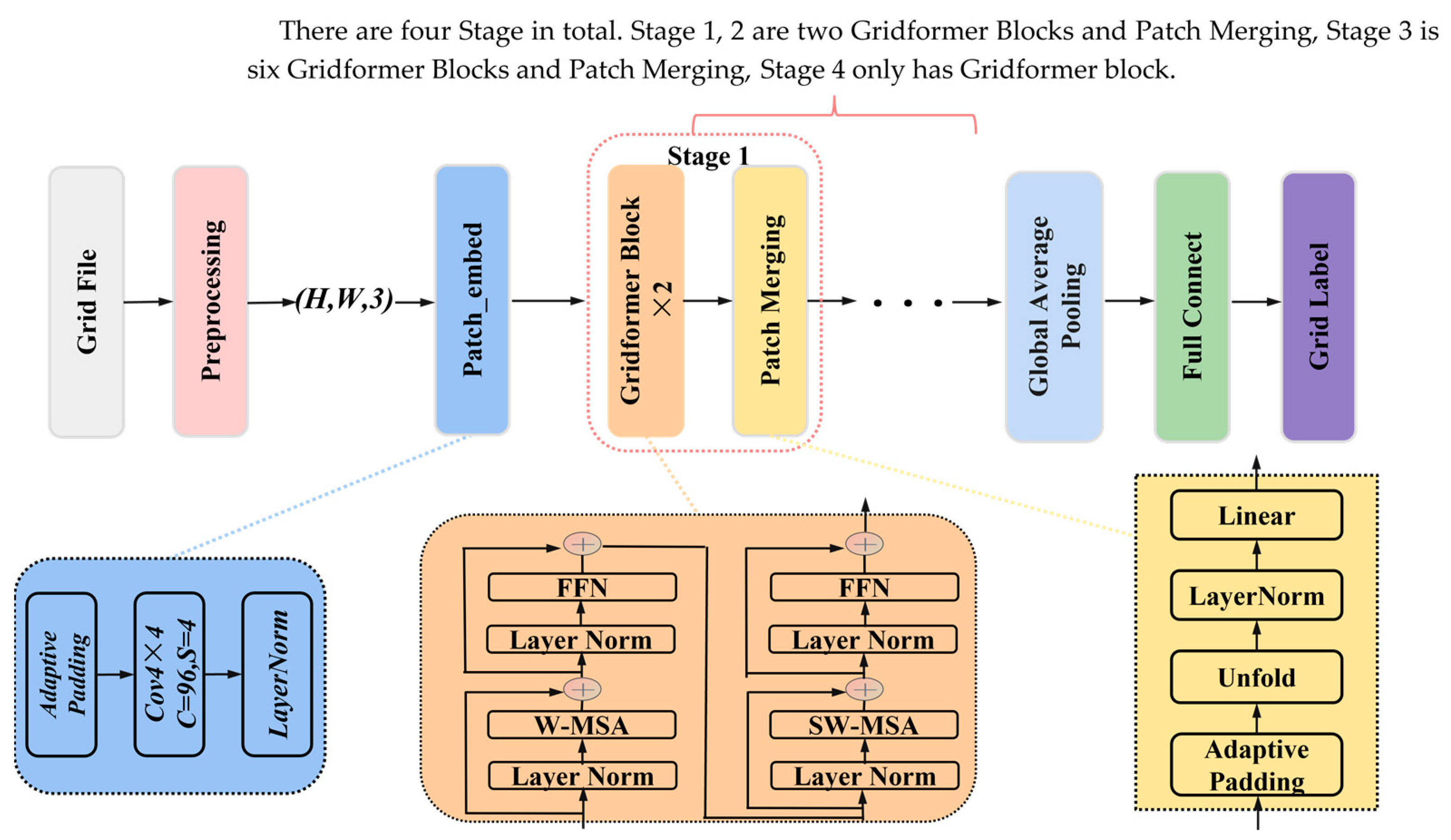
The NACA-Market dataset is designed with different sizes of airfoil meshes for generality. But the Transformer structure of the network requires a fixed size of input data. Gridformer can train different sizes with our designed algorithm, whose structure is shown in Figure 4.

Gridformer architecture mainly consists of Patch_embed, Gridformer Block, Patch Merging, and Full Connect to form a hierarchical structure to obtain feature maps of different sizes. It ultimately uses the Global Average Pooling and Full Connect layers to transform the data and output the mesh quality categories. The Patch_embed module is to divide the input data into a certain number of Patches and then maps each Patch onto a one-dimensional vector by linear mapping. The input data format token required by the model is implemented in principle by convolutional layers. As shown in Figure 4, the four stages are composed of Gridformer Block and Patch_Merging. These stages have different numbers of Gridformer Blocks, which are 2, 2, 6, and 2, respectively. Each Gridformer Block is composed of Layer Normalization (Layer Norm) [41], Windows Multi-Head Self-Attention (W-MSA) [42], Shifted Windows Multi-Head Self-Attention (SW-MSA) [42], and Feed Forward Network (FFN). W-MSA and SW-MSA are used in pairs in the module, where W-MSA reduces the calculation amount and SW-MSA enables the communication between adjacent windows as a way to extract multi-scale feature maps. FFN executes a linear transformation of the features, the main structure is shown in Figure 5, consisting of Linear, activation function GELU, and Dropout.

The Patch Merging module performs downsampling and consists of AdaptivePadding, Unfold, Layer Norm, and Linear, as shown in Figure 4. It is added in Stage 1, Stage 2, and Stage 3, in order to continuously enlarge the receptive field. It makes the network focus on the local features of the mesh while taking into account the global information of the mesh.

In summary, Gridformer first preprocesses and normalizes the mesh data into a 3D matrix for input into the network, and the 3D matrix is converted into a token data format by Patch_embed. Then, it uses four stage modules to obtain the nonlinear relationship between mesh features and their labels, with feature channels varying between 96 and 3072. Lastly, the extracted features are compressed using a Global Average Pooling layer and a Fully Connect layer into a 1 × 8 feature map, which is output as the prediction result of the mesh. Layer Norm and the activation function GELU in the module are used to accelerate the training of the model and prevent overfitting and gradient disappearance. In addition, relative position encoding is incorporated, and pre-trained weights provided in OpenMMlab [43] are used to improve the accuracy of the prediction.

3.3. Gridformer Block

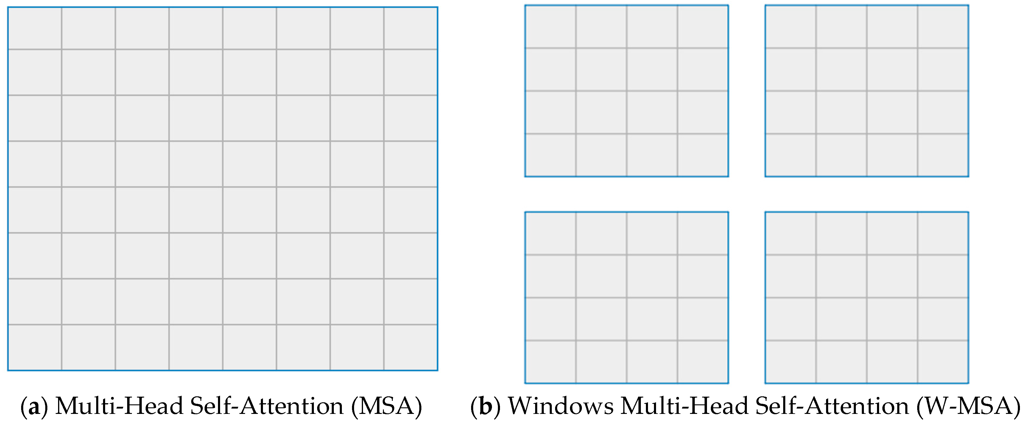
The standard Transformer structure performs a global self-attention calculation when classifying images, called MSA. Specifically, the relationship between one token and all other tokens is calculated, which results in a squared increase in the amount of computation. Moreover, since the structure cannot extract multi-scale features, it is less suitable for mesh quality evaluation. To evaluate the mesh quality more efficiently, feature maps of different sizes are extracted. The Gridformer Block module is built in this paper, which mainly consists of W-MSA and SW-MSA. W-MSA is based on the concept of the window, which can effectively reduce the calculation amount by calculating self-attention only within the window. As shown in Figure 6, a gray square represents the feature vector corresponding to a patch, and the whole graph is the feature map of the graph. Figure 6a shows that each token in the feature map needs to be computed with all other tokens during the MSA computation on self-attention. W-MSA in Figure 6b, the feature map is first divided into individual Windows according to M × M size; M is the size of each window. The self-attention is performed separately for each Windows internal. The formula for comparing the calculated quantities of the two is as follows:

$$\Omega \left(\mathrm{MSA}\right)=4hw{C}^2+2{\left(hw\right)}^2$$

(7)

$$\Omega \left(\mathrm{W}-\mathrm{MSA}\right)=4hw{C}^2+2M^{2}hwC$$

(8)

In Equations (7) and (8), $h$ and $w$ are the height and width of the feature map, respectively, which are usually large values. $C$ is the depth of the feature map. $M$ is the specified window size, the general size is 7. After introducing the W-MSA mechanism, the calculation amount is reduced by tens or even hundreds of times.

Figure 6. Multi-Head Self-Attention and Windows Multi-Head Self-Attention. (a) Self-attention is computed for the whole feature map, which is computationally intensive. (b) The whole feature map is divided into four windows, and the self-attention in each window is computed in parallel, reducing the calculation amount and improving the computational efficiency.

Figure 6. Multi-Head Self-Attention and Windows Multi-Head Self-Attention. (a) Self-attention is computed for the whole feature map, which is computationally intensive. (b) The whole feature map is divided into four windows, and the self-attention in each window is computed in parallel, reducing the calculation amount and improving the computational efficiency.

W-MSA solves the memory and calculation amount problems well. But each window computes its self-attention independently of the others, does not communicate with the others, and no longer has the ability to model globally. The SW-MSA mechanism was introduced to enable interaction between its windows. Comparing Figure 7a,b, the windows are shifted from four windows to nine windows, completing the communication of data between different windows. For example, the shaded portion of the window in Figure 7b is composed of shaded portions of the different windows in Figure 7a.

While solving the problem that information cannot interact between different windows, the windows are converted from four windows to nine windows after shifting. The size of the nine windows is not consistent, resulting in the inability to compute self-attention quickly, increasing the calculation amount. The elements between different windows are mixed after the sliding window. As the self-attention calculation requires interconnected elements, the evaluation of quality attributes such as smoothness, orthogonality, and spacing distribution cannot be conducted. The problem is solved by using a mask for self-attention calculation. As shown in Figure 7c, the slide-out window is shifted and transformed into four windows of the same size, then the region that should not do the self-attention calculation is masked. The principle is to subtract a relatively large number from the value of the matrix calculated from the region and take the value of 0 from softmax. Finally, the window is restored to Figure 7b to ensure that the original position information is not changed.

To obtain the connection of mesh adjacencies and to better assess the quality of the mesh, position coding is added. The existing position encoding methods consist of two types, namely absolute position encoding [33] and relative position encoding [38]. Absolute position encoding adds a position encoding for each patch, and relative position encoding adds a position encoding when doing the self-attention calculation. After comparison, the performance is significantly improved by using relative position encoding in Gridformer, which is calculated as follows:

$$Attention\left(Q,K,V\right)=SoftMax\left(Q{K}^T/\sqrt{d}+B\right)V$$

(9)

where

$$Q,K,V\in R^{M^2\times d},B\in R^{M^2\times M^2}$$

In Equation (9), Q, K, and V, respectively, represent the query matrix, key matrix, and value matrix, obtained by multiplying the input three-dimensional matrix by each of the three weight matrices. $d$ is the dimension of the query, key matrix. $M^2$ is the number of Patches in the window. $B$ is the relative position bias matrix, which is directly added to the attention matrix.

3.4. Dynamic Input Size

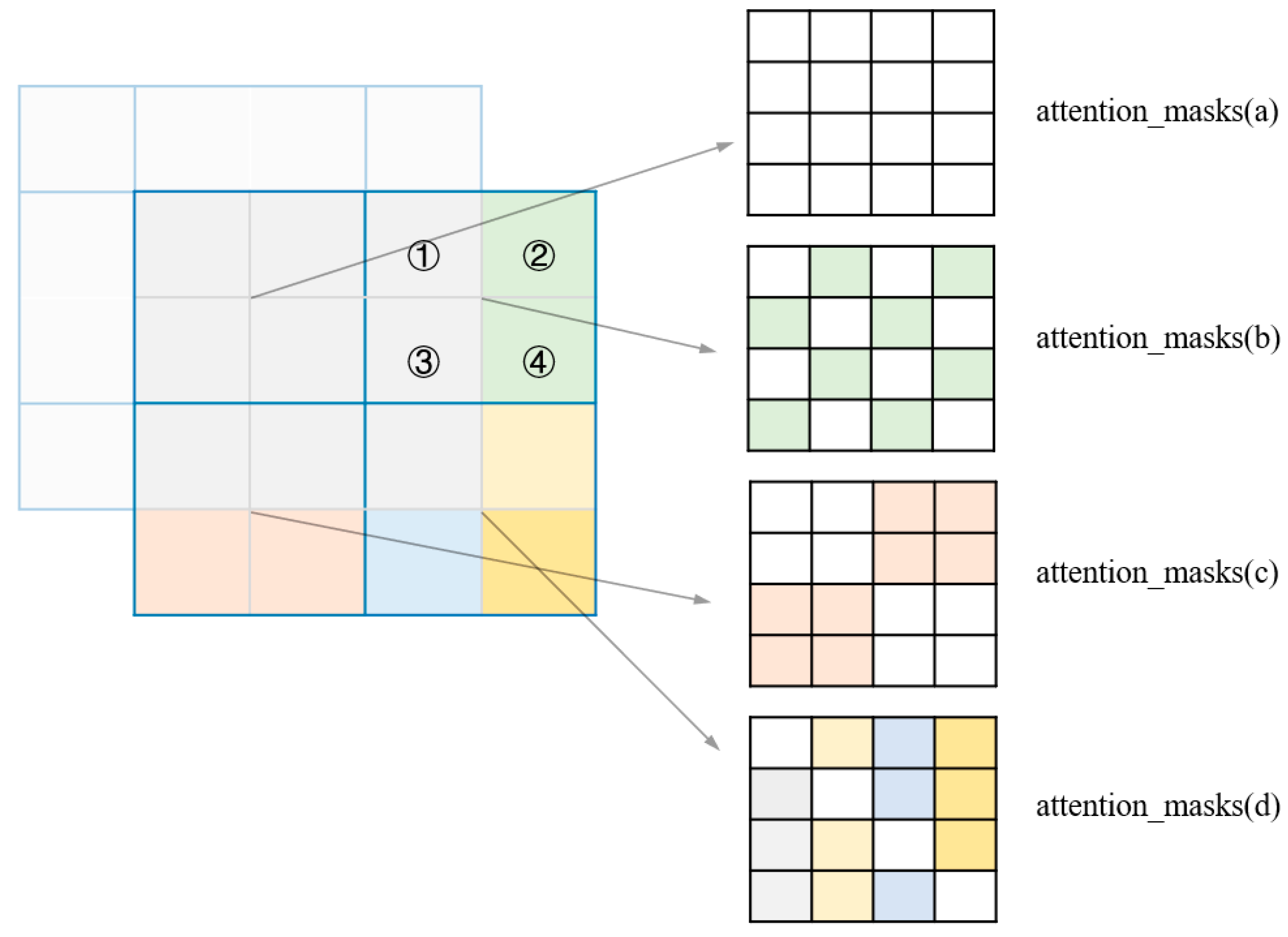
In networks for image classification, CNN structure-based networks usually do not need to specify the size of the input image. Transformer structure-based networks need to specify the input image size parameters during the building process. Since the relative position encoding confined to the inner window is used to match the window attention mechanism, when we change the size of the input image, it will not affect the relative position encoding inside the window. But the number of windows may be changed, involving the mask in the self-attention calculation in the SW-MSA mechanism. To easily understand how the mask is generated, we use the example of a smaller feature map (4 × 4) and a smaller window (2 × 2), as shown in Figure 8.

According to the mechanism of SW-MSA, the feature map was windowed, and nine windows were generated. After shifting the feature map and combining some of the windows, four windows of the same size were generated for the self-attention calculation. Each window in Figure 8 corresponds to a window combination case that requires a different mask to calculate attention. Taking “attention_masks(a)” as an example, the corresponding 4 × 4 feature window has only the first row and the first column in gray. When calculating the feature ①, only ① and ③ features are considered, and the features calculated between ② and ④ will be masked. The green part of the figure represents the eight masks being generated. As a result, how many masks need to be generated depends on how many windows are available after window splitting. The content of each mask relies on the form of the edge window combination within the corresponding window. To achieve dynamic input size, the problem that the mask is difficult to calculate when the size of the overall feature map and the number of windows change needs to be overcome. The algorithm is designed to dynamically generate the corresponding mask depending on the input image size during the forward propagation performed by Gridformer. The results demonstrate that the calculated amount using this method is reasonable and does not involve complex interpolation operations. The implementation of dynamic mesh size input makes Gridformer generic enough to be used to evaluate the quality of other mesh types.

4. Experiment

4.1. Data Preparation

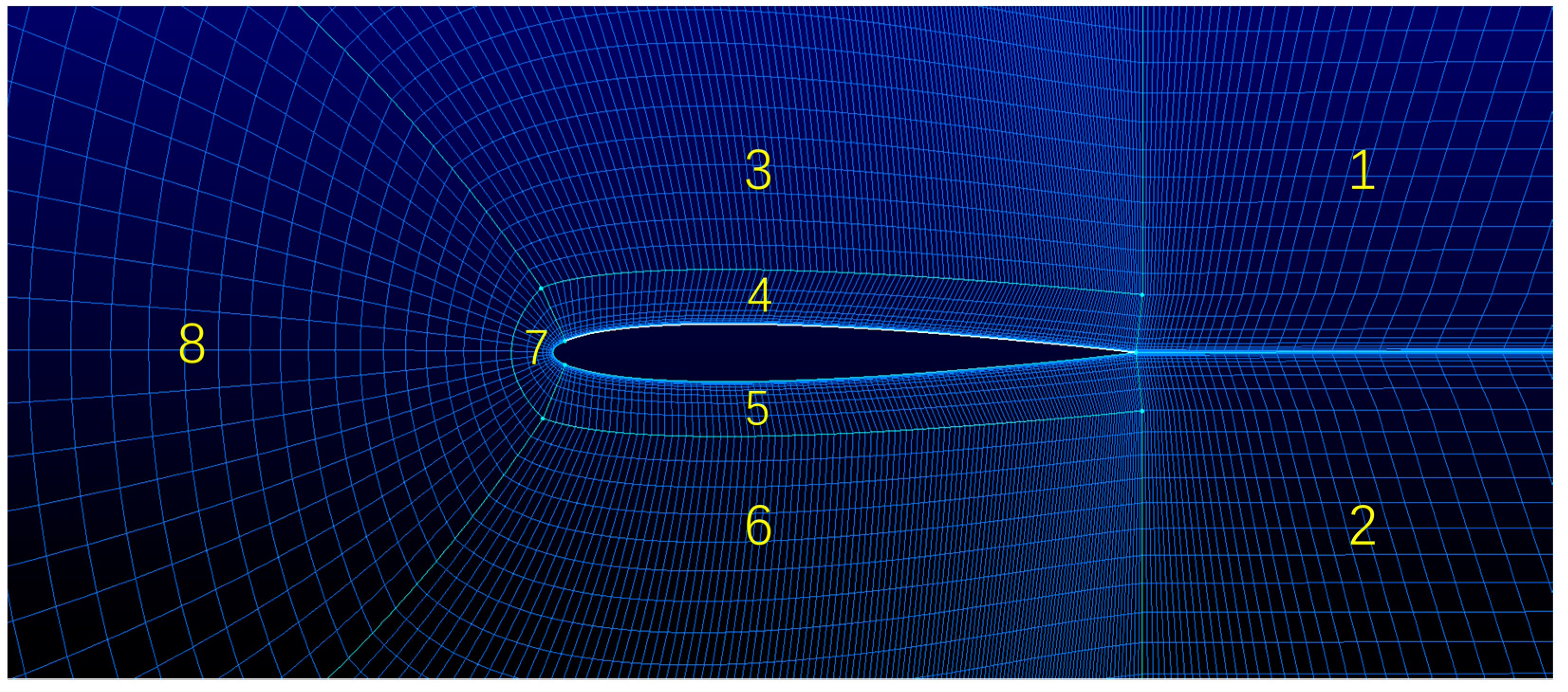
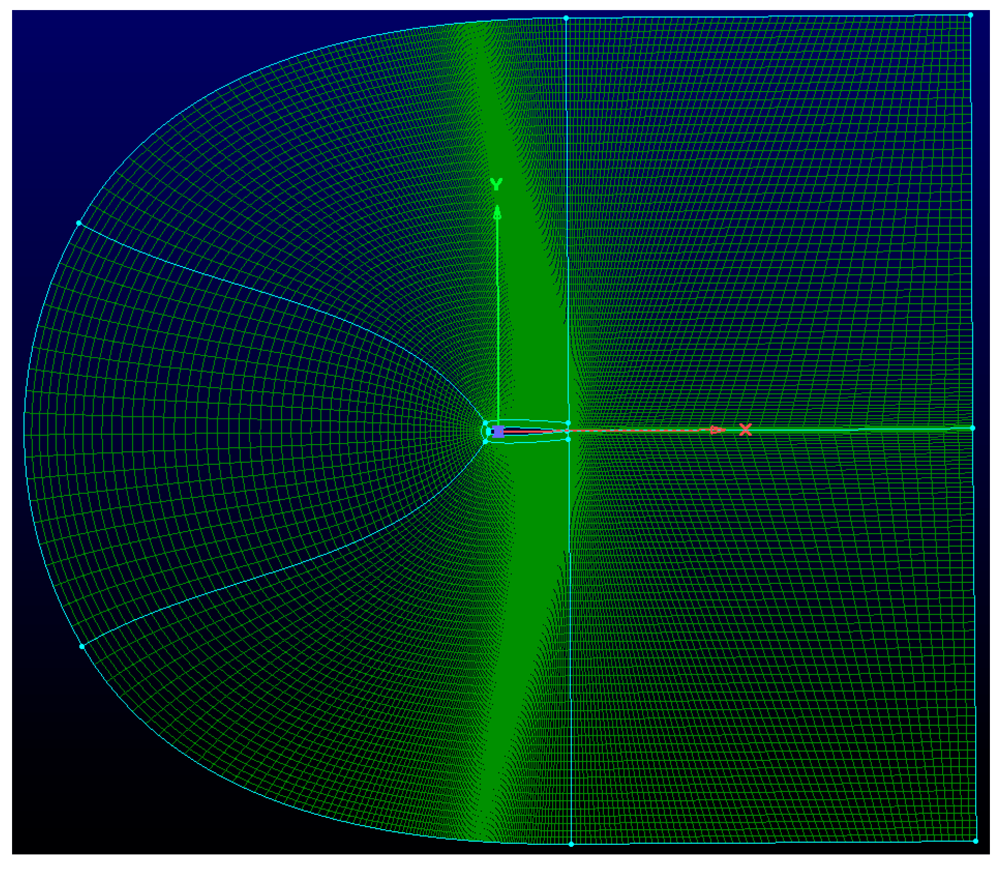
For Transformer-supervised training types of neural networks, large datasets with accurate labels are required for training to identify important features. In this section, an airfoil benchmark dataset NACA-Market is introduced to train the Gridformer. NACA-Market is a two-dimensional structured mesh dataset on NACA-0012 Airfoil for solving mesh quality evaluation problems. There are 10,240 airfoil meshes in total. An example of the geometric model with topology is shown in Figure 9. Since the airfoil mesh in NACA-Market is generated using eight regions, we divide it into eight faces.

For the generality of the dataset, the mesh data were set in different sizes. According to

Table 1. Different size meshes.

No.	Mesh Size	Number
1	80 × 380	1024
2	82 × 384	1024
3	84 × 388	1024
4	86 × 392	1024
5	88 × 396	1024
6	90 × 400	1024
7	92 × 404	1024
8	94 × 408	1024
9	96 × 412	1024
10	98 × 416	1024

[24], NACA-Market contains 10 sizes of airfoil meshes, ranging from 80 × 380 to 98 × 416, and each size contains 1024 meshes.

According to the criteria for a high-quality airfoil mesh, different areas of the mesh need to have proper orthogonality, smoothness, and spacing distribution. Based on these three properties, we manipulate a good mesh into eight different quality categories by modifying the points and lines. As listed in

Table 2. Different types of meshes.

Label	Name	Label	Name
1(W)	Well-shaped	5(P-OS)	Poor orthogonality and smoothness
2(P-O)	Poor orthogonality	6(P-OD)	Poor orthogonality and distribution
3(P-S)	Poor smoothness	7(P-SD)	Poor smoothness and distribution
4(P-D)	Poor distribution	8(P-OSD)	Poorly shaped

[24], it includes well-shaped, poor orthogonality, poor smoothness, poor density, poor orthogonality and smoothness, poor orthogonality and density, poor smoothness and density, and poorly shaped, each of which has 1280 sets of meshes.

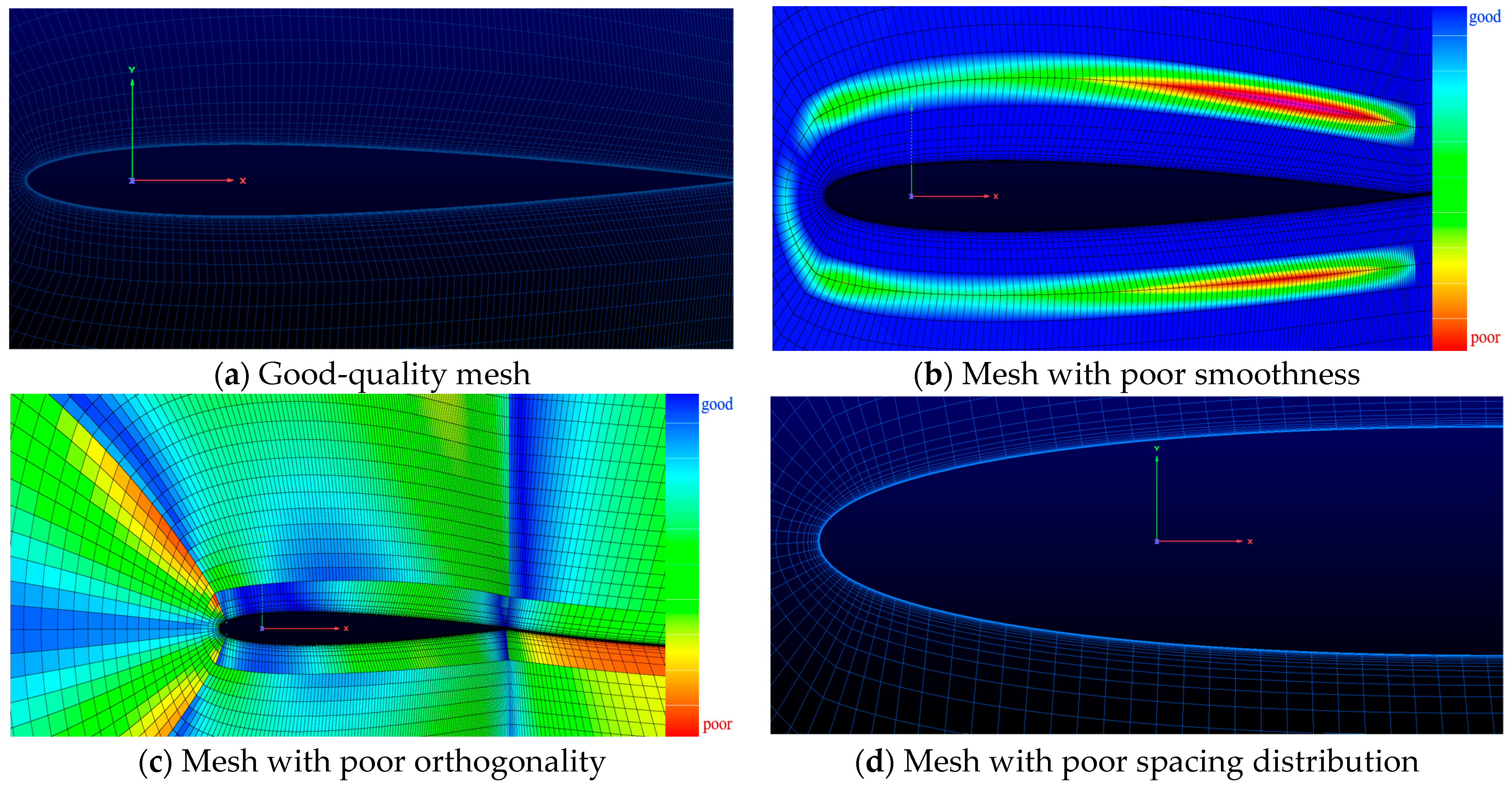
To more clearly distinguish between meshes of different quality, a sample of several meshes with poor quality properties is provided in Figure 10.

The purpose of refining the mesh classes is to provide clear guidelines for the mesh optimization process and to improve the mesh quality by corresponding algorithms. For example, meshes with poor orthogonality can be optimized using topological transformation or local transformation; meshes with poor smoothness can be optimized using mesh smoothing algorithms; and meshes with poor spacing distribution can be optimized using local refinement.

It is well known that the scale of the dataset affects the learning performance of the Transformer; thus, data augmentation is often used to expand the data volume. In this paper, we adopted mirror and randomflip to augment the dataset. Other commonly used approaches such as crop, lighting, cutmix, and mixup can destroy the data linkage of the mesh itself and are not suitable for application in mesh quality evaluation. The augmented dataset was divided into 80% and 20% for Gridformer training and testing, respectively.

4.2. Training Process

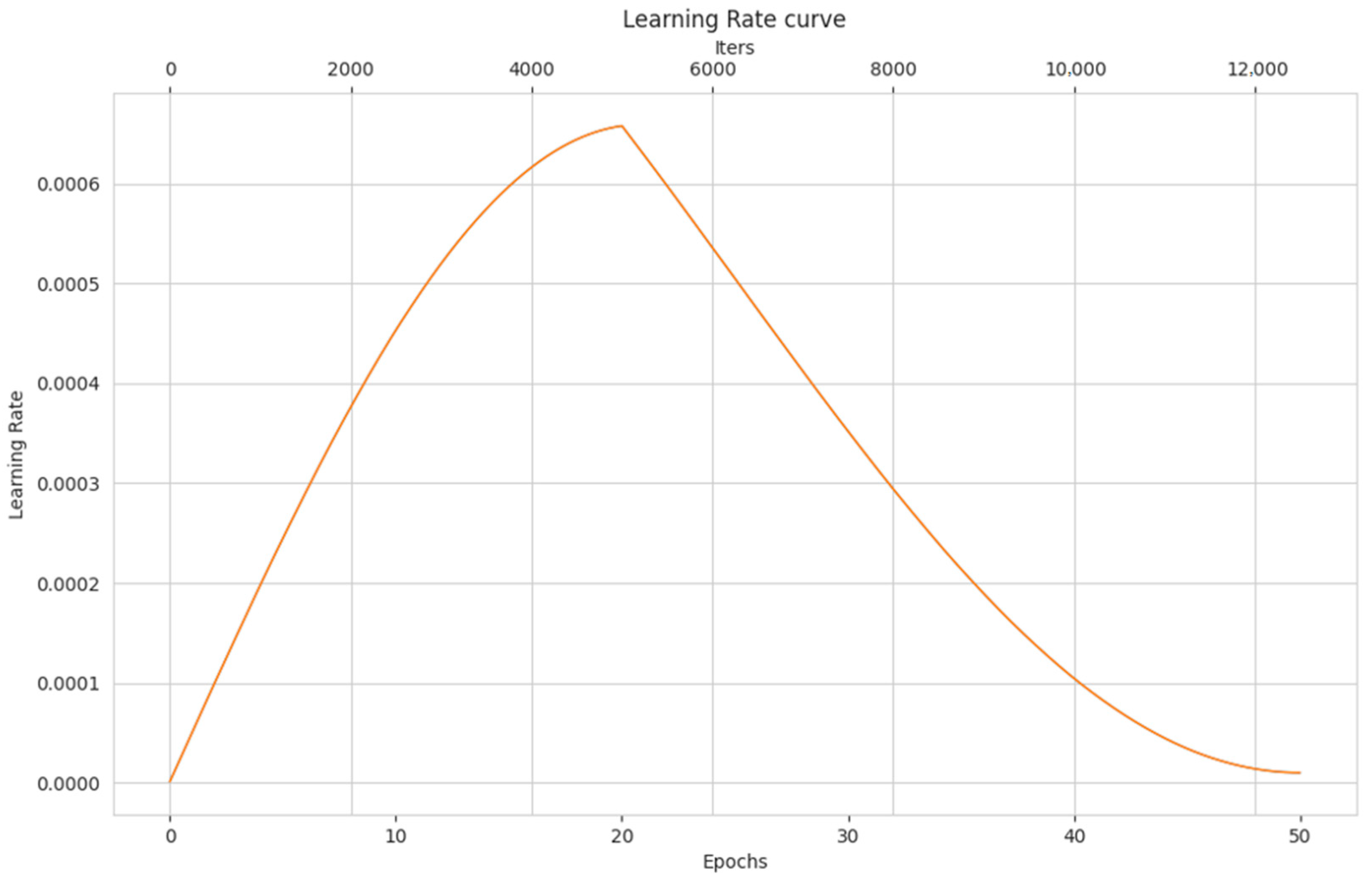
We chose the Adam WeightDecay (AdamW) [44] Optimizer to perform adaptive gradient descent optimization, which can improve the model generalization, accelerate gradient descent, and adaptively adjust the learning rate. The training was started with a learning rate of 0.001, a weight decay of 0.05, eps set to 10⁻⁸, and betas = (0.9, 0.999). Since the network is unstable at the beginning of training, setting a small learning rate directly may deteriorate the prediction results. The learning rate strategy of cosine annealing with warm_up was chosen to enhance the prediction accuracy. As shown in Figure 11, the learning rate increases linearly from a very small number to a preset learning rate and then decays according to the cosine function value. Label Smoothing Cross Entropy was used as the loss function. The batch size was set to 64, and the number of iterations was set to 50. A NVIDIA 3090 GPU was used to train the proposed network during the whole experiment.

In Section 3.1, we mentioned that to ensure the interpretability and reliability of the mesh feature extraction, five feature groups are composed based on the geometric properties of the mesh cells as shown in

Table 3. The weight percentage of features and the prediction results of feature groups.

No.	Feature Group	Proportion of Weight	Accuracy
1	(Lx, Ly, Ma)	(0.37, 0.36, 0.27)	94.93%
2	(Dx, Dy, Ma)	(0.226, 0.224, 0.45)	91.64%
3	(Rls, Rd, Ma)	(0.42, 0.27, 0.31)	93.22%
4	(Rls, S, Ma)	(0.33, 0.39, 0.28)	95.61%
5	(Rd, S, Ma)	(0.30, 0.37, 0.33)	93.71%

, including the length L_x, the length L_y, length D_x of the diagonal, length D_y of the diagonal, the diagonal ratio R_d, the ratio R_ls of the longest side to the shortest side, the area S of the mesh cell, and the maximum interior angle M_a of the mesh. Each feature group consists of different properties, with the aim of exploring the impact of different features on the prediction results and finding a feature group that best represents the mesh. Considering having angle information to discriminate orthogonality, we choose to keep the maximum interior angle. The feature group is used as a three-channel matrix for the input Gridformer. A weight parameter is added to each channel of the matrix, and the percentage value of each channel feature is viewed at the last layer of the Gridformer after training. For each type of mesh cell, Table 3 shows the weight percentage of the geometric features in the feature group.

The experimental results demonstrated that the weights of the diagonal lengths D_x and D_y and the diagonal ratio R_d are less than 0.3, which indicates a relatively low impact on the mesh quality evaluation. Instead, the weights of L_x, L_y, R_ls, and S are all above 0.3. In terms of accuracy comparison, Group 4 (ratio R_ls of longest to shortest edges, area S of the cell mesh, and maximum angle M_a) has the highest prediction accuracy of 95.61%. Group 2 has the lowest prediction accuracy of 91.64%. Therefore, in the subsequent experiments, the fourth feature group has been chosen as the input into the Gridformer.

4.3. Network Evaluation Results

In this section, we have conducted three sets of experiments. The first set of experiments is a comparison of the prediction results of Gridformer and GridNet for eight mesh quality categories. The purpose of the experiments is to verify that Gridformer based on Transformer is more suitable for mesh quality evaluation. The second set of experiments is a comparison of Gridformer with neural networks commonly used in deep learning. The purpose of the experiments is to verify the high accuracy and low overhead of Gridformer. The third set of experiments is a comparison of Gridformer with ICEM CFD based on the traditional quality metric to evaluate the mesh quality results. The purpose of the experiments is to verify the superiority of Gridformer.

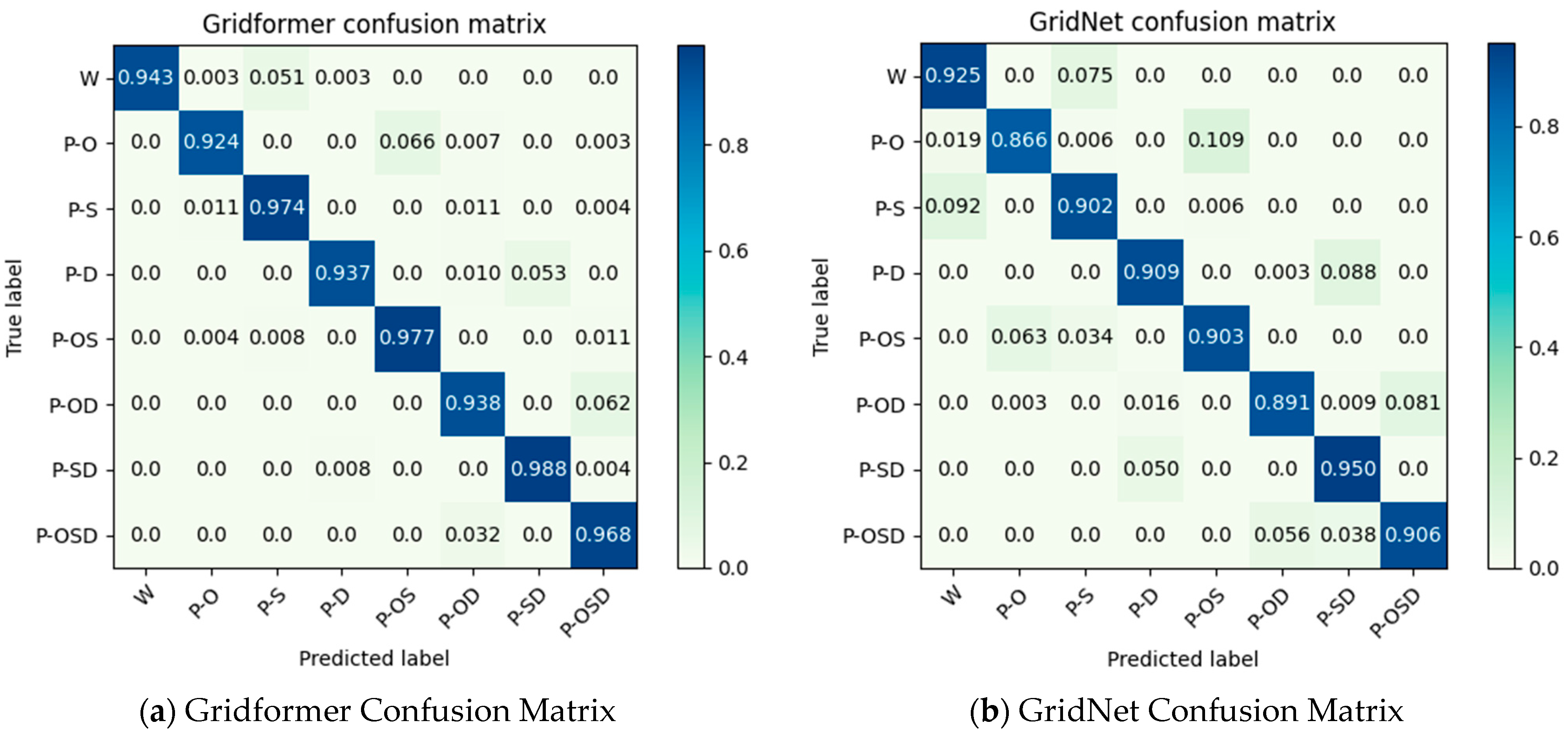
First, we evaluated the accuracy of the network on the NACA-Market dataset. To better analyze the accuracy between different quality categories, the confusion matrix of Gridformer and GridNet is given for comparison.

As shown in Figure 12, the prediction accuracy of Gridformer was above 92% for all categories. In particular, Gridformer significantly improved the accuracy of the P-OS and P-S categories by 7.4% and 7.2%, respectively, compared to GridNet. This shows that Gridformer is better at identifying the local features of the mesh. For the category P-SD, both Gridformer and GridNet achieved the highest prediction accuracy, 98.8% and 95%, respectively. This validates that Gridformer based on Transformer is more suitable for evaluating mesh integral features.

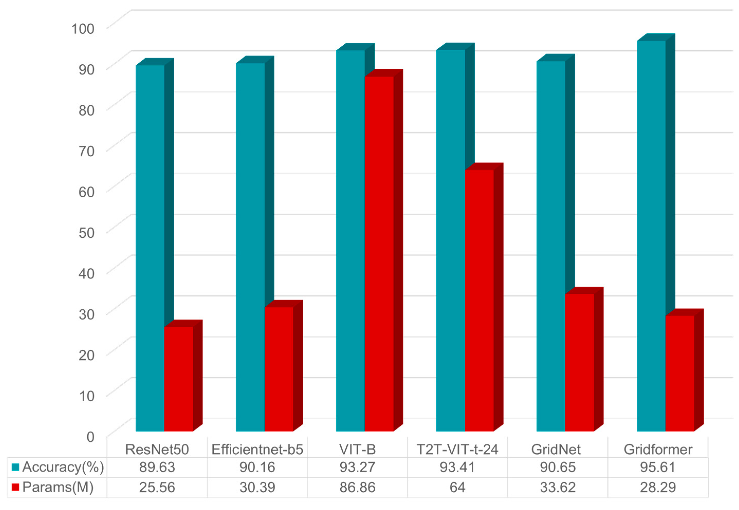
Second, we also trained several commonly used neural networks (ResNet [45], Efficientnet [46], VIT [36], T2T-VIT [47]) and GridNet for comparison with Gridformer. As shown in Figure 13, although the networks of the Transformer series all possess relatively good prediction results in terms of accuracy, GridNet, which is designed for mesh quality evaluation, has the advantages of low parameter overhead and high accuracy. The accuracy of Gridformer proposed in this paper achieves the highest prediction accuracy of 95.61% on NACA-Market compared to another commonly used neural network. There is an enhancement of 4.96% compared to GridNet. More importantly, the parameter overhead is only 28.29M, a 15.86% reduction compared to GridNet. The 95.61% accuracy and 28.29M parameter overhead prove the high accuracy and high efficiency of Gridformer. Specifically, Comparing the 200 iterations of GridNet training, Gridformer requires only 50 epochs. It dramatically reduces mesh quality evaluation time and provides timely prediction results for subsequent tuning work.

In an experimental environment with an NVIDIA 3090 GPU, an epoch took only 46.4 s. If, in a multi-GPU distributed training environment, the training time for mesh evaluation is further reduced, better interacting with tuning would greatly facilitate the development of mesh automation.

Finally, to verify that the proposed Gridformer model can accurately identify different mesh quality defects, we compare the results with those of the widely used ICEM CFD software’s quality evaluation based on traditional metrics for mesh geometry properties. The visualization of the results of the evaluation of two airfoil meshes with quality defects in the dataset is shown in Figure 14. Figure 14a shows that the traditional metric identifies regions of poor orthogonality and poor smoothing in the mesh sample. However, this traditional evaluation method may not accurately identify some meshes that have defects. In Figure 14b, the actual sample of meshes with poor spacing distribution is evaluated by the traditional quality metric as good quality meshes and no over-spacing of the mesh boundary layers is identified. Compared with traditional techniques, Gridformer is not only able to learn quality features related to mesh orthogonality and smoothness, but also to identify spacing distribution errors in the boundary layers. It demonstrates that Gridformer can provide an effective evaluation for mesh integrity quality.

After comparing the results with the traditional quality metric, it is confirmed that Gridformer can capture the potential errors of low-density meshes and correctly classify them into meshes with poor spacing distribution. Experiments demonstrate that the network is more reliable than traditional quality evaluation methods.

In summary, Gridformer can automate quality evaluation with high accuracy while reducing computational and storage overhead. The evaluation process not only considers the influence of geometric features on the mesh cells, and orthogonality, but also the properties between the integral mesh, smoothness, and spacing distribution. It also demonstrates better evaluation capabilities than the traditional mesh quality evaluation.

4.4. Analysis of the Hyperparameters

The adjustment of hyperparameters makes a critical contribution to the performance of the model by reducing computational overhead and improving accuracy. However, the training process requires manual debugging, which is time-consuming. In this paper, two hyper-parameters, the optimizer and the depth of the model, which have a large impact on the network performance, are discussed. In experiments, we fix other parameters, choose different optimizers, and change the depth of the network.

As shown in Figure 15, the loss of the AdamW optimizer decreases the fastest and converges gradually after 50 epochs of training, while the losses of the Stochastic Gradient Descent (SGD) and Nesterov Acceleration Gradient (NAG) optimizers decrease relatively more slowly.

Up through the end of 100 epochs,

Table 4. Comparison of accuracy of different optimizers.

Optimizers	Epoch50_Accuracy	Epoch100_Accuracy
SGD	88.63%	93.34%
NAG	91.25%	95.89%
AdamW	95.61%	95.61%

demonstrates that NAG achieves an accuracy of 95.89%, which is slightly higher than AdamW.

However, NAG requires manual tuning of the parameters to find the optimal learning rate, while AdamW can adaptively adjust the optimizer for the learning rate and is more generalized. Since mesh quality evaluation requires timely interaction, and generalization to other topologies is desired, the AdamW optimizer has been chosen for its faster convergence and better generalization capabilities.

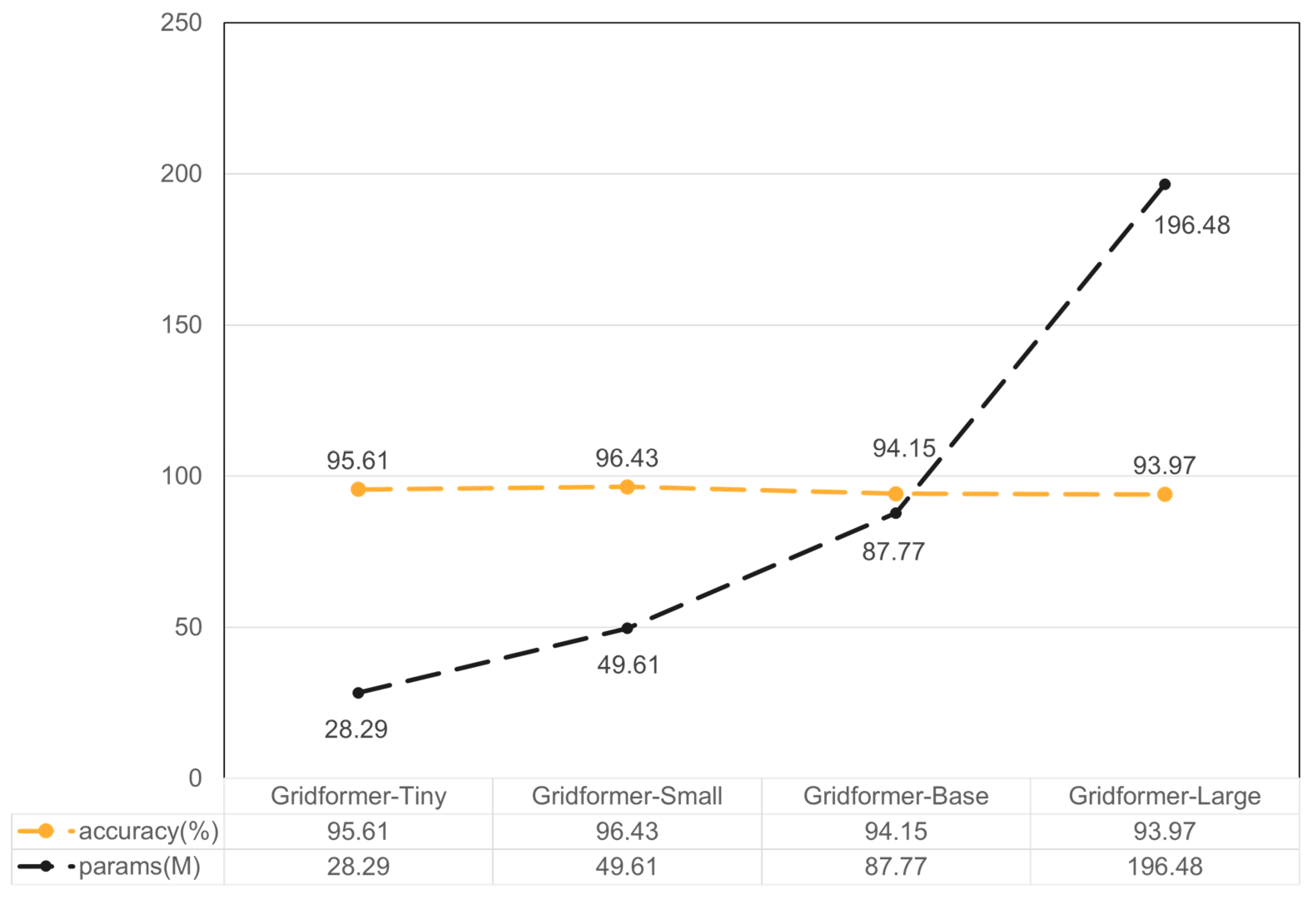
In addition, the depth of the network is changed by increasing Gridformer Block, the number of heads in the multi-head attention module, and the channel depth of the feature map in the experiment. Gridformer-Tiny takes 2, 2, 6, 2 Gridformer Blocks; Gridformer-Small, Gridformer-Base, and Gridformer-Large all take 2, 2, 18, 2 Gridformer Blocks. The initial number of heads is 2, 3, 4, and 6, and the initial channel depth is 96, 96, 128, 192, respectively. The experimental results are shown in Figure 16.

Although Gridformer-Small achieves the highest prediction accuracy of 96.43%, the parameter overhead increases with it. It is tuned for faster evaluation results to obtain a high-quality mesh. We choose Gridformer-Tiny, which has a lower parameter overhead, with an accuracy of 95.61%.

The above is a series of experiments on the performance of Gridformer. Specifically, we analyze the impact of Gridformer with different optimizers and different scale sizes on the comprehensive performance of the model. The results illustrate that Gridformer is an efficient and high-precision method for automatic mesh quality evaluation.

4.5. A Workflow for Generating High-Quality Meshes Based on Gridformer

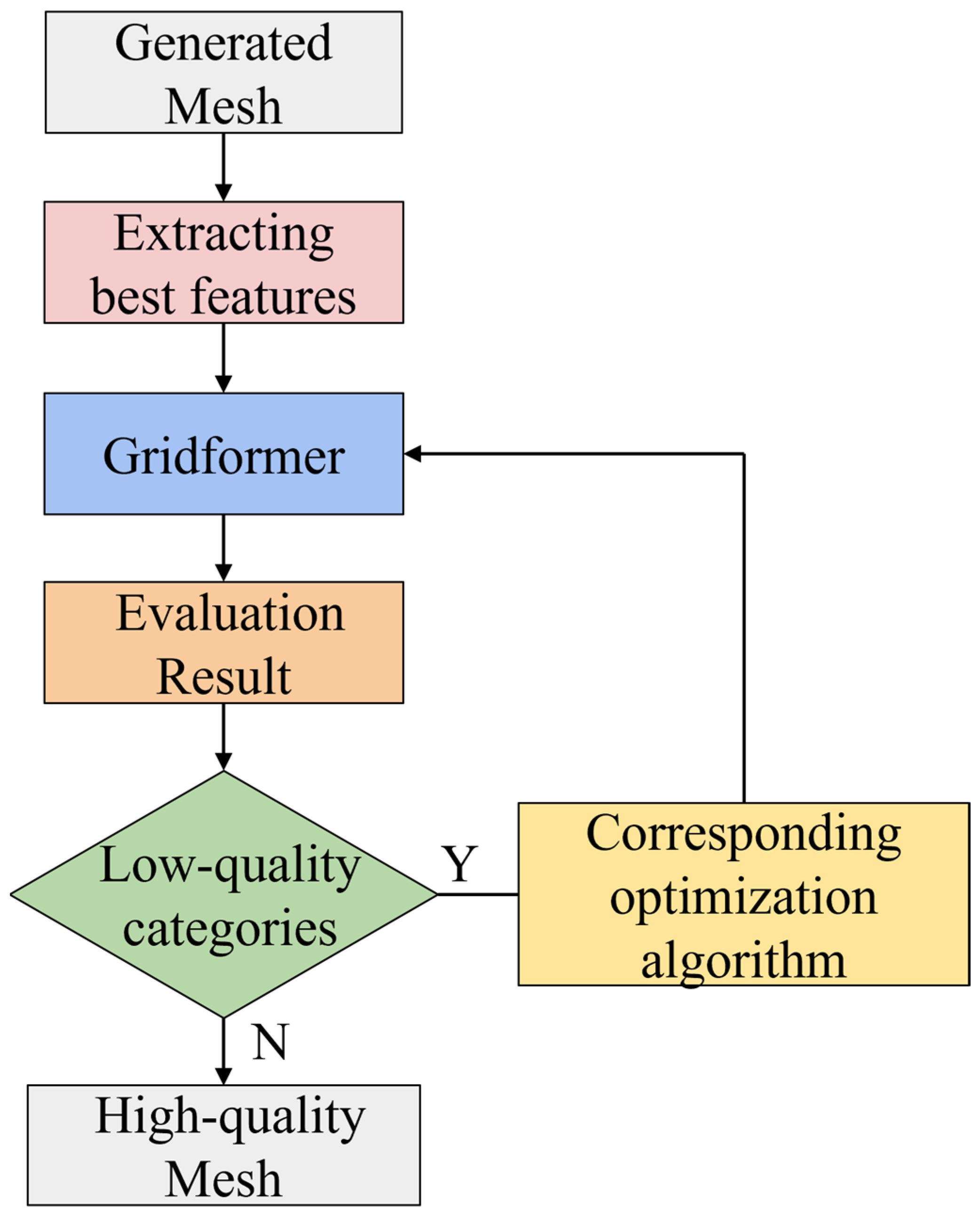
The quality of the mesh determines the accuracy of the numerical solution. Obtaining a high-quality mesh requires the frequent intervention of CFD professionals, including the selection of control parameters for the initial mesh partitioning, manual evaluation of mesh quality, and tuning. So, mesh quality evaluation is a highly specialized task. The biggest challenge that hinders the fully automated generation of high-quality meshes is the time-consuming and labor-intensive process of mesh quality evaluation. A Gridformer-based workflow for high-quality mesh generation is presented for this purpose (see Figure 17). Mainly, the trained Gridformer model is embedded into the process, and the high-quality mesh is generated fully automatically according to the quality categories predicted by the network combined with the corresponding mesh optimization algorithm.

The workflow for automating the generation of high-quality meshes is divided into a total of four steps: (1) generating the initial mesh; (2) extracting the best features by comparison; (3) output network evaluation quality categories, such as mesh smoothness, orthogonality, and spacing distribution; (4) the results of (3) combined with the corresponding mesh optimization algorithm for mesh tuning. The above process is repeated until the mesh quality is met to standard. The entire workflow can be generated–evaluated–tuned fully automatically without human involvement, improving the efficiency of mesh quality evaluation and reducing labor costs.

We detail the mesh optimization algorithm of the above step (4). A mesh with poor orthogonality can be optimized by topology transformation [48]. A mesh with poor smoothness can be optimized by a mesh smoothing algorithm [49]. A mesh with poor spacing distribution can be optimized by local refinement [50]. In addition, a corresponding evaluation and algorithm optimization can also be performed based on the mesh quality category that is set.

To verify the reliability and practicality of the workflow, the airfoil mesh from NACA-Market is inputted into Gridformer for automatic evaluation. A new mesh is generated after tuning according to the obtained mesh quality category and the corresponding optimization algorithm. Two approaches are taken to verify that the quality of the optimized mesh is enhanced: (1) re-evaluating it with Gridformer; (2) comparing the aerodynamic properties calculated with the theoretical values. The results show that the optimized mesh is re-evaluated as a high-quality mesh, and the aerodynamic properties are generally consistent with the theoretical values.

The low-quality airfoil meshes are significantly improved by the automatic evaluation and tuning with the participation of Gridformer. High-quality meshes generated automatically through the workflow are shown in Figure 18, which proves the utility of the workflow.

5. Conclusions

Mesh post-processing is a complex task that is usually performed by CFD professionals. The core of this task is mesh quality evaluation to ensure that the mesh is of sufficient quality to achieve accurate numerical simulations. Mesh quality evaluation has become a bottleneck for automatic mesh generation, as it is time-consuming and labor-intensive.

In this paper, Gridformer is designed to automate mesh quality evaluation by learning the quality properties between the mesh cells and the integral mesh. First, the degree of influence of different features on mesh quality evaluation was explored in the process, and the best three features are selected, including ratio R_ls of longest to shortest edges, area S of the cell mesh, and maximum angle M_a, which provide a degree of interpretability and reliability. Next, the neural networks commonly used in deep learning and the evaluation results of ICEM CFD are compared. Last, Gridformer is added to the high-quality mesh generation workflow. According to the results of mesh evaluation combined with the corresponding optimization algorithm, automated mesh generation is promoted. The experimental results demonstrate that Gridformer can identify mesh quality defects that cannot be identified by traditional mesh quality metrics. Gridformer outperforms other neural networks, achieving the highest prediction accuracy of 95.61% and the lowest computational overhead of 28.29 M.

Future work includes developing specific loss functions and performance measures in conjunction with the mesh itself, properties to better guide the training of the model and improve its performance. It is also hoped that during the training process, potential features representing the mesh will be discovered to contribute to common mesh quality criteria. In addition, the desired Gridformer-based high-quality mesh generation process can facilitate automated mesh generation.