A Proton Flux Prediction Method Based on an Attention Mechanism and Long Short-Term Memory Network

Abstract

Accurately predicting proton flux in the space radiation environment is crucial for satellite in-orbit management and space science research. This paper proposes a proton flux prediction method based on a hybrid neural network. This method is a predictive approach for measuring proton flux profiles via a satellite during its operation, including crossings through the SAA region. In the data preprocessing stage, a moving average wavelet transform was employed to retain the trend information of the original data and perform noise reduction. For the model design, the TPA-LSTM model was introduced, which combines the Temporal Pattern Attention mechanism with a Long Short-Term Memory network (LSTM). The model was trained and validated using 4,174,202 proton flux data points over a span of 12 months. The experimental results indicate that the prediction accuracy of the TPA-LSTM model is higher than that of the AP-8 model, with a logarithmic root mean square error (logRMSE) of 3.71 between predicted and actual values. In particular, an improved accuracy was observed when predicting values within the South Atlantic Anomaly (SAA) region, with a logRMSE of 3.09.

1. Introduction

When it comes to the safety and operational stability of satellite spacecraft, the significance of the space radiation environment cannot be underestimated. The radiation present in space, such as high-energy particles, solar storms, and cosmic rays, profoundly impacts various aspects of satellite spacecraft.

Numerous studies focused on assessing the impact of space radiation on satellite electronic components. For instance, as demonstrated by N Ya’acob et al.’s [1] research, high-energy particle impacts may result in Single-Event Effects (SEE) and Total Ionizing Dose (TID) in electronic elements. These events can lead to temporary or permanent malfunctions of electronic devices, subsequently affecting satellite performance and functionality. DJ Cochran et al. [2] extensively examined the sensitivity of various candidate spacecraft electronic components to Total Ionizing Dose and displacement damage.

In the context of investigating the impact of space radiation on satellite spacecraft, proton flux stands as a crucial component of space radiation that holds undeniable significance. Both its energy and quantity can exert notable effects on satellite electronic components, thereby influencing satellite performance and operational stability. Numerous scholars have conducted pertinent research in this realm. For instance, R Uzel et al. [3] explored the efficiency of localized shielding structures in capturing protons to meet reliability requirements. S Katz et al. [4] observed an elevated single-event upset rate in the low Earth orbit polar satellite Eros B as high-energy proton flux increased.

However, merely understanding variations in the radiation environment falls short; accurate predictions and warnings are equally crucial. The proton flux data during satellite operation represent a stable time series. Predicting this time series not only provides crucial data references for space science research but also offers vital insights for satellite operation and management, thereby preventing malfunctions and instability in high-radiation environments.

In this regard, a substantial amount of research has been devoted to exploring how to construct more accurate radiation environment prediction and warning methods. For instance, J Chen et al. [5] introduced an embedded approach for forecasting Solar Particle Events (SPE) and Single-Event Upset (SEU) rates. This approach enables prediction through the increase in SEU count rates one hour prior to the forthcoming flux changes and corresponding SPE events.

In the realm of space radiation environments, particularly in the prediction of proton flux, although machine learning methods offer a promising avenue, they also encounter a series of challenges. Firstly, the complexity of the data amplifies the difficulty of prediction tasks [6]. Secondly, the presence of various noises could disrupt predictive models, impacting the accuracy of forecasts [7]. Most significantly, the accuracy of predictive models stands as a key challenge [8].

In recent years, deep learning methods have made significant progress in handling time series data for this issue. These methods include Convolutional Neural Networks (CNN) [9,10,11], ARMA Neural Networks [12], and Long Short-Term Memory Networks (LSTM) [13,14,15], among others [16]. For instance, L Wei et al. [17] used a Long Short-Term Memory Network (LSTM) to develop a model for predicting daily > 2 MeV electron integral flux in geostationary orbit. Their model takes inputs such as geomagnetic and solar wind parameters, as well as the values of the >1 MeV electron integral flux itself over the past consecutive five days. Their experimental results indicated a substantial improvement in predictive efficiency using the LSTM model compared to some earlier models. The predictive efficiencies for the years 2008, 2009, and 2010 were 0.833, 0.896, and 0.911, respectively.

In the realm of deep learning, attention mechanisms stand as powerful tools [18,19]. These mechanisms allow models to focus on crucial time segments, enhancing accuracy in predicting future trends. In the field of space radiation environment prediction, the application of attention mechanisms is gaining traction. For instance, X Kong et al. [20] introduced a Time Convolutional Network model based on an attention mechanism (TCN-Attention) for predicting solar radiation. Their experimental results underscore the strong predictive performance of their proposed model, with a Nash-–Sutcliffe Efficiency coefficient (NSE) of 0.922.

Building upon the foundation of attention mechanisms, SY Shih et al. [21] introduced Temporal Pattern Attention (TPA), a technique with distinct advantages in time series prediction. TPA can be employed to identify pivotal time segments within proton flux time series which might correspond to specific intervals when satellites traverse certain spatial positions. By accentuating these key time segments, the model becomes more adept at capturing the changing patterns of radiation events, consequently enhancing predictive performance.

In the prediction of space radiation environments, the combination of wavelet transform and neural network models can yield excellent predictive results [22]. Data processed through wavelet transform can exhibit strong predictive performance in the realm of space radiation, enhancing the model’s accuracy in forecasting radiation events [23]. For instance, SS Sharifi et al. [24] employed Continuous Wavelet Transform (CWT) in conjunction with a Multi-Layer Perceptron Neural Network (MLPNN) to predict Solar Radiation (SR). The results showcased the outstanding predictive performance of the CWT-MLPNN approach, with the R2 coefficient increasing from 0.86 to 0.89 compared to using a standalone MLPNN.

This paper presents a hybrid neural network model for predicting proton flux profiles measured via a satellite during its operation, including crossings through the SAA region. The model integrates the data preprocessing, hybrid neural network prediction, and accuracy verification steps. The data are processed using moving average wavelet transform, and the model incorporates latitude and longitude features, along with a Temporal Pattern Attention (TPA) mechanism. For this paper, building upon the LSTM neural network, a hybrid neural network model was constructed, and our experimental results demonstrate that the TPA-LSTM model exhibits good predictive performance in forecasting proton flux profiles.

2. Methods

2.1. Overall Method and Evaluation Criteria

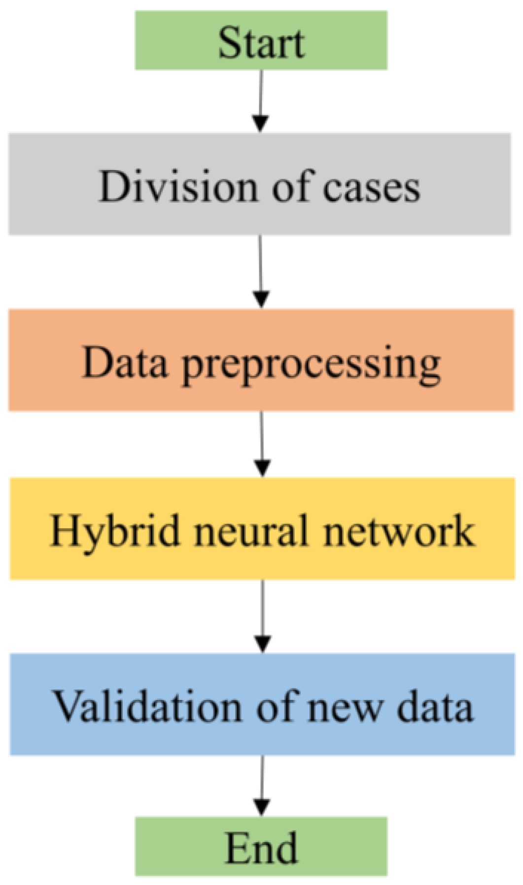
The objective of this study was to predict space radiation proton flux using a hybrid neural network model. The model integrates multiple techniques, as depicted in Figure 1, encompassing data preparation and data preprocessing, hybrid neural network prediction, and accuracy verification and discussion.

We initially divided the dataset into 26 cases, randomly selecting 15 for the training set while leaving the rest for validation. During the data preprocessing phase, we employed moving average wavelet transform, marking our first innovation. This involved calculating the trend component of the data using the moving average method and denoising and decomposing the data using wavelet analysis. Subsequently, we analyzed proton flux data and identified the South Atlantic Anomaly (SAA) region as an area of significant fluctuation. This became our entry point for introducing latitude and longitude features and attention mechanisms, our second innovation. Following this, we constructed a hybrid neural network model, encompassing two LSTM layers, a TPA layer, and a dropout layer. In this step, our third innovation was the adoption of the TPA-LSTM model. Finally, we designed a series of experiments to verify the model’s accuracy. We primarily focused on the model’s accuracy in predicting proton flux for all time steps, particularly emphasizing its accuracy in predicting within the SAA region. Through comparisons with other models, we demonstrated the TPA-LSTM model’s accuracy in forecasting space radiation proton flux and showcased its performance across various time series prediction tasks.

For this paper, we employed two evaluation metrics to assess the predictive performance of the model: logRMSE (Logarithm of Root Mean Squared Error) and logMAE (Logarithm of Mean Absolute Error). Given the substantial differences in magnitude between the proton flux data in this study, we used logRMSE and logMAE as evaluation metrics. logRMSE is calculated by computing the mean of the logarithmic differences between predicted values and observed values. This mitigates the impact of data magnitude differences, ensuring that errors at larger scales do not unduly influence the evaluation metrics. logMAE, on the other hand, first takes the logarithm of each prediction error and then calculates their averages. Logarithmic error can shift the focus of the evaluation process towards relative error rather than absolute error. The formulas for both metrics are as follows:

$$logRMSE=\ln (\sqrt{\frac{1}{n}\times {\displaystyle \sum _{i=1}^n{\left(y_i-{\widehat{y}}_i\right)}^2}})$$

(1)

$$logMAE=\ln (\frac{1}{n}\times {\displaystyle \sum _{i=1}^n\left|y_i-{\widehat{y}}_i\right|})$$

(2)

In Equations (1) and (2), $n$ is the number of samples, ${\widehat{y}}_i$ is the predicted value, $y_i$ is the actual value.

2.2. Data Preparation and Dataset Partition

The in-orbit satellite-measured proton flux data in this study were provided by Shanghai SastSpace Technology Co., Ltd. The energy range of high-energy protons was 100.00 MeV to 275.00 MeV. The satellite was identified as 52085, and its orbital elements are presented in

Table 1. Six orbital elements of the satellite 52085.

Element	Value
Semi-major axis	7395 km
Eccentricity	0.01°
Inclination	63.398°
Perigee argument	41.145°
RAAN	132.892°
Mean anomaly	319.739°
Orbital period	105.47 min

. The satellite employs Si detectors, with a shielding effect equivalent to 1 mm of Al. This study considers the measured proton flux data for this satellite from April 2022 to March 2023.

We partitioned the dataset into 26 distinct time periods, providing the time period number, start time, end time, and duration for each time period, and all time periods involve crossings through the SAA region, as outlined in Appendix A 

Table A1. Detailed information of time periods.

No.	Time Range	Duration (min)
1	2022/04/17 22:37–2022/04/18 12:09	671
2	2022/04/24 10:33–2022/04/25 11:07	1394
3	2022/05/07 09:30–2022/05/08 11:26	1405
4	2022/05/09 08:58–2022/05/10 10:58	1440
5	2022/08/11 08:28–2022/08/13 07:56	2867
6	2022/08/13 07:56–2022/08/15 07:24	2871
7	2022/08/15 07:24–2022/08/17 06:52	2877
8	2022/08/17 06:52–2022/08/19 06:20	2887
9	2022/08/19 06:20–2022/08/21 05:48	2891
10	2022/08/25 04:44–2022/08/27 04:11	2870
11	2022/08/27 04:11–2022/08/29 03:39	2870
12	2022/09/02 02:35–2022/09/04 02:03	2870
13	2022/09/04 02:03–2022/09/06 01:31	2877
14	2022/09/06 01:31–2022/09/08 00:59	2877
15	2022/09/17 01:33–2022/09/19 00:41	2877
16	2022/11/16 10:33–2022/11/18 10:00	2877
17	2022/11/18 10:00–2022/11/20 09:28	2668
18	2022/11/20 09:28–202211/22 08:56	2672
19	2022/11/22 08:56–2022/11/24 08:24	2672
20	2022/11/24 08:24–2022/11/26 07:52	2668
21	2022/12/02 23:51–2022/12/04 23:19	2668
22	2022/12/06 22:47–2022/12/08 22:15	2668
23	2022/12/18 19:34–2022/12/20 10:11	1757
24	2023/01/01 21:08–2023/01/03 20:36	2870
25	2023/02/16 12:46–2023/02/18 12:13	2877
26	2023/02/18 12:13–2023/02/20 06:22	2528

. Among the 26 cases, a subset of 15 cases were randomly selected for training purposes, while the remaining 11 were exclusively reserved for validation in each predictive iteration. To mitigate the influence of inherent randomness stemming from the selection of training and testing sets, along with the variability in parameter configuration, we conducted a minimum of 50 independent runs for each specific method to accurately portray their predictive accuracy. All evaluation metrics were derived from the predictive data generated by the validation set and compared against actual observations.

2.3. Data Preprocessing

During the data preprocessing stage, we employed the moving average wavelet denoising method. This process involves calculating the data’s trend component using the moving average technique, applying wavelet transformation for noise reduction, and selecting appropriate wavelet bases and decomposition levels. The result is a processed time series dataset. The processing procedure is illustrated in Figure 2.

In the data preprocessing process, we initially employed the moving average method to compute the trend component of the data. The moving average method is a commonly used smoothing technique that reduces noise and retains trend information by calculating the mean within a sliding window. By calculating the trend component, we can better grasp the overall trend of the data and reduce interference in subsequent analysis and modeling. The formula for the moving average method is as follows:

$$T_t=m/{\displaystyle \sum _{j=-k}^k{y}_{t+j}}$$

(3)

In the above equation, $y_t$ represents the time series data, $m=2k+1$, meaning that the trend at time t is derived by calculating the average of $y_t$ over the preceding and succeeding k cycles. This method is referred to as “m-MA”, denoting an m-order moving average. To achieve an even-order moving average, we performed two consecutive odd-order moving averages.

We proceeded with wavelet transformation, harnessing the potent capabilities of this signal processing tool. During the satellite’s operational phases, it may traverse specific zones, such as the South Atlantic Anomaly (SAA), or encounter space weather events like solar proton events, resulting in sudden magnitudes of proton flux data increase. Wavelet transformation facilitates the retention of these crucial data points while enabling a beneficial decomposition, thus aiding the learning process of neural networks. We adopted the minimax thresholding approach of wavelet transformation to establish the thresholds. Data points with trend values computed through the moving average method that surpass the threshold were designated as noise. Rooted in the distribution traits of wavelet coefficients, this method gauges noise by contrasting the amplitude of wavelet coefficients with the threshold. It constitutes a simple yet effective signal processing technique, proficiently eliminating noise while retaining vital information. The threshold is determined by an empirical formula:

$$\lambda =\left\{\begin{array}{c}0,N\le 32\\ 0.3936+0.1829\ln (N-2),N>32\end{array}\right\}$$

(4)

where N represents the length of the input sequence.

2.4. Long Short-Term Memory Network (LSTM)

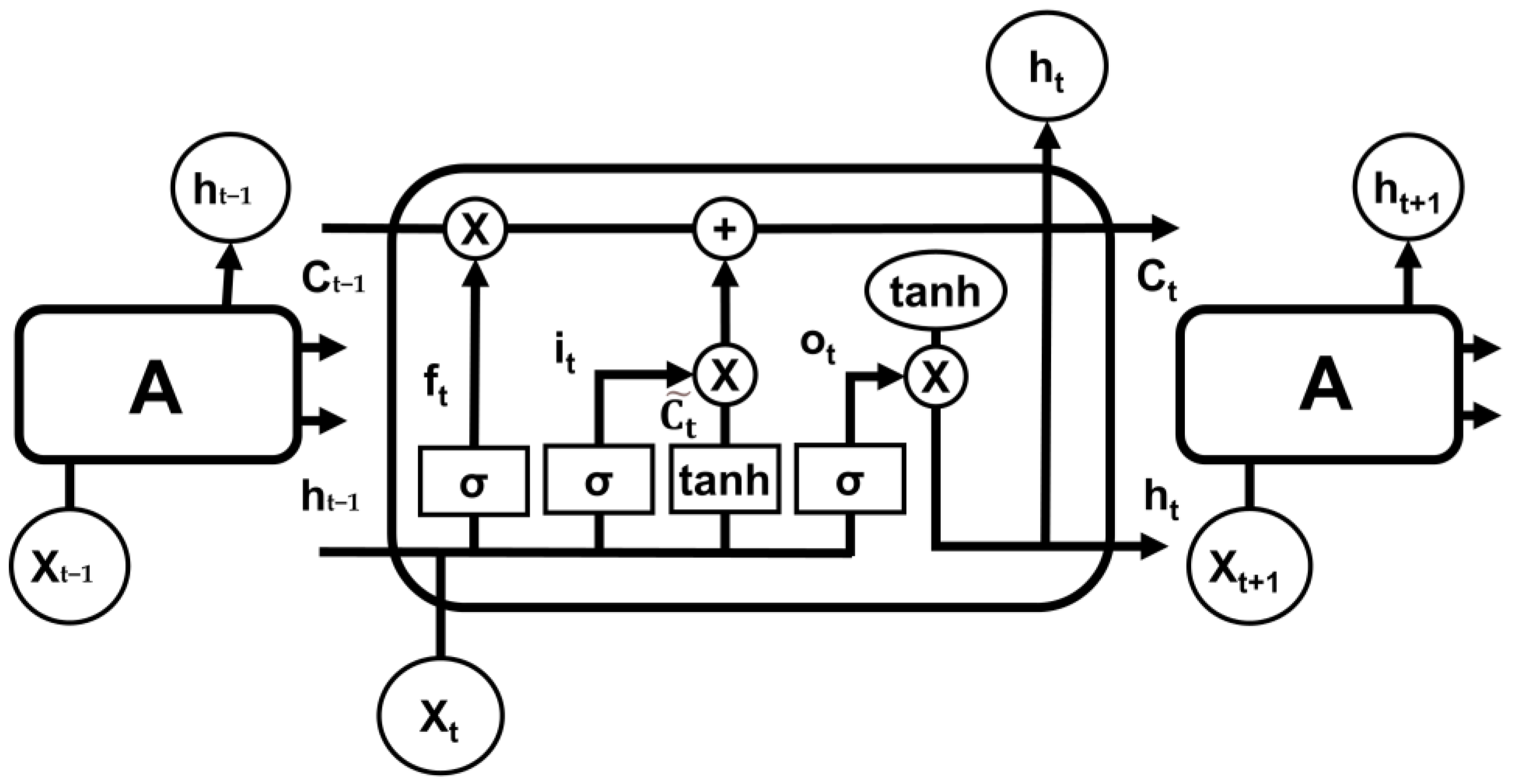
Long Short-Term Memory (LSTM) is a variant of the traditional Recurrent Neural Network (RNN). In handling longer time sequences, conventional RNNs often encounter issues with long-term dependencies, leading to the omission of information between distant time steps and subsequently causing performance degradation. LSTM, however, exhibits enhanced memory capabilities, allowing it to learn and capture long-term dependencies effectively, thereby facilitating more efficient information transmission within the time sequence. When dealing with time sequences, LSTM outperforms, enabling the model to better capture intricate relationships within time sequence data. This improvement in capturing complex associations heightens the accuracy and efficacy of time series modeling.

Figure 3 illustrates the structure of the LSTM model comprising three LSTM units, each denoted as Unit A. Within each LSTM layer, the neural units receive inputs from the current input $X_t$, the output $h_{t-1}$ of the preceding LSTM unit, and the cell state vector $C_{t-1}$ of the previous LSTM unit. Meanwhile, the output of the neural units encompasses the cell state vector $C_t$ of the current LSTM layer’s memory unit at time t, as well as the output $h_t$ of the current LSTM unit at time t.

The internal neural structure of the LSTM network is depicted in Figure 3. Each LSTM layer acts as a robust memory cell, regulating the flow and retention of information through a forget gate $f_t$, an input gate $i_t$, and an output gate $o_t$.

The forget gate plays a crucial role in LSTM, determining which information from the current time step input $X_t$ and the output $h_{t-1}$ of the previous LSTM unit should be retained and which should be forgotten. By passing through a sigmoid activation function, the forget gate outputs a value between 0 and 1. A value close to 1 indicates that the information will be retained, while a value close to 0 signifies that the information will be forgotten. This allows LSTM to selectively keep important information and discard less relevant details, effectively addressing long-term dependencies in time series and enhancing sequence modeling and prediction performance. The formula is as follows:

$$f_t=\sigma (W_f[X_t,h_{t-1}+b_f])$$

(5)

In Equation (5), $W_f$ is the weight of the forget gate, and $b_f$ is the offset of the forget gate.

The input gate in LSTM is utilized to update the cell state. Its calculation process is as follows: Firstly, the current input $X_t$ is passed through a sigmoid activation function, along with the output $h_{t-1}$ of the previous LSTM unit, to obtain the control value $i_t$. This control value’s output ranges from 0 to 1, where 0 signifies unimportant and 1 represents important. Subsequently, the current input $i_t$ and the output $h_{t-1}$ of the previous LSTM unit are put through a tanh function to generate a new state information $\tilde{C}$. The value of $\tilde{C}$ also lies between 0 and 1, representing the effective information of the current LSTM unit. The control value $i_t$ determines the degree to which the information in $\tilde{C}$ is integrated into the cell state $\tilde{C}$. Then, the previous cell state $C_{t-1}$ is updated to the new cell state $C_t$. Initially, the forget gate $f_t$ is multiplied by the previous cell state $C_{t-1}$, allowing for selective forgetting of certain information. Next, the input gate it is multiplied by $\tilde{C}$ to obtain the updated cell state vector $C_t$. This process achieves the selective updating of the cell state, efficiently transmitting vital information. The formulas are as follows:

$$i_t=\sigma (W_i[X_t,h_{t-1}+b_i])$$

(6)

$$\tilde{C}=\tan \mathrm{h}(W_c[X_t,h_{t-1}+b_c\left]\right)$$

(7)

$$C_t=f_t\times C_{t-1}+i_t\times \tilde{C}$$

(8)

In Equations (6) and (7), $W_i$ and $b_i$ are the weight and bias of the input gate; $W_c$ and $b_c$ are the weight and bias of the control unit.

The output gate, denoted as $o_t$, is employed to regulate the output $h_t$ of the current LSTM unit at the given time step. Initially, the extent of the output gate’s opening is computed using a sigmoid activation function, resulting in an output control value ranging between 0 and 1. Then, the new cell state $C_t$ obtained from the input gate is passed through the tanh function, producing an output between −1 and 1. Lastly, the output of the tanh function is multiplied by the output control value of the output gate to yield the final output $h_t$. This way, the output gate can flexibly determine which components of the cell state $C_t$ will influence the output $h_t$ at the current time step. The formulas are as follows:

$$o_t=\sigma (W_o[X_t,h_{t-1}+b_o])$$

(9)

$$h_t=o_t\times \tan (C_t)$$

(10)

In Equation (9), $W_o$ and $b_o$ are the weights and offsets of the output gate.

2.5. Temporal Pattern Attention (TPA)

Temporal Pattern Attention (TPA) is an advanced attention mechanism designed for capturing temporal dependencies and patterns in time series data. The model structure is illustrated in Figure 4. In this study, TPA demonstrates the capability to selectively focus on variations in latitude and longitude features during the South Atlantic Anomaly (SAA) region, which represents time periods of greater significance for changes in radiation proton flux. This adaptability enhances the model’s precision in predicting variations in radiation proton flux.

TPA is typically connected after an LSTM layer. Initially, the hidden state matrix $H=\left\{h_{t-w},h_{t-w-1},\mathrm{\dots }{h}_{t-1}\right\}$, where $w$ represents the sliding window length, is obtained from the LSTM layer’s output. Sequence features are extracted by performing convolutional operations using CNN filters $C=\left\{C_1,C_2,\mathrm{\dots }{C}_T\right\}$, with a total of T filters. The convolution operation between $H$ and $C$ results in the temporal pattern matrix $H^C$. The formula is as follows:

$$H_{i,j}^C={\displaystyle \sum _{l=1}^w{h}_{i,(t-w-1+l)}\times C_{j,T-w+l}}$$

(11)

where $H_{i,j}^C$ represents the result of the action of the $i$th row vector and the $j$th filter in the hidden state matrix.

Next, the similarity between time steps is calculated through a scoring function. In TPA, the attention mechanism employs a “Query-Key-Value” mechanism to compute attention weights. In this mechanism, Query is used to inquire about the relevance of specific time steps, Key is utilized to compute the similarity between different time steps, and Value encompasses the features of time steps. By employing a scoring function to compute the similarity between Query and Key, attention weights for each time step can be derived, thus achieving weighted aggregation across different time steps. In this context, the LSTM layer’s output $h_t$ serves as the Query, the temporal pattern matrix $H^C$ functions as the Key, the calculation of relevance between $h_t$ and $H^C$ is conducted, and normalization using the sigmoid function yields the attention weights ${\alpha }_i$. The formulas are as follows:

$$f(H_i^C,h_t)={\left(H_i^C\right)}^T{h}_t$$

(12)

$${\alpha }_i=\mathrm{sigmoid}(f(H_i^C,h_t\left)\right)$$

(13)

The third step involves weighted aggregation. Weighted aggregation refers to the process of computing the weighted sum of Values based on attention weights to obtain the final context vector $V_t$. Here, Value signifies the hidden state information of each time step, which corresponds to the temporal pattern matrix $H^C$. This weighted representation highlights significant time steps, thereby extracting crucial temporal patterns. The formula is as follows:

$$V_t={\displaystyle \sum _{i=1}^N{\alpha }_i{H}^C}$$

(14)

where $N$ is the length of the sequence.

Lastly, the weighted representation obtained from TPA, $V_t$, is integrated into further computations of the model. The influence of the context vector $V_t$ on the current output $h_t$ is incorporated into $h_t$, resulting in the ultimate output $h_t{}^{\prime }$. The formula is as follows:

$$h_t{}^{\prime }=W_h{h}_t+W_v{V}_t$$

(15)

where $W_h$ is the weight of the current output state, and $W_v$ is the weight of the context vector.

3. Results and Discussion

3.1. Moving Average Wavelet Transform

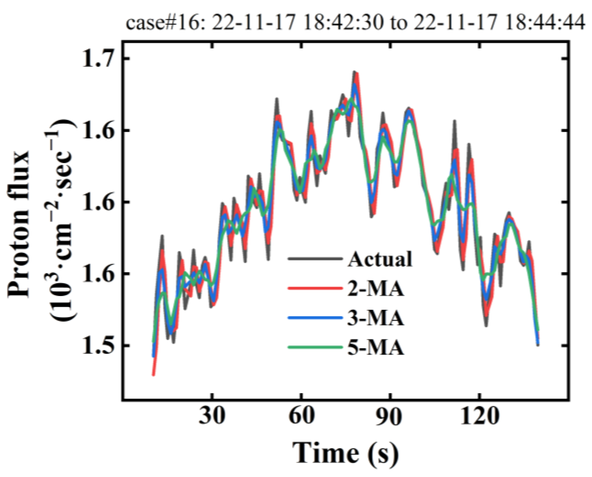
Firstly, we applied the moving average method to obtain the trend component of the original proton flux data. To select an appropriate moving average order, denoted as m, we experimented with different orders, including 2, 3, and 5. As observed from Figure 5, the trend component curve derived using the moving average method effectively captures the primary directional trend of the time series. As m increases, the moving average curve gradually approaches a smoother state due to larger m values, leading to more data smoothing. To better preserve the fluctuation pattern of the original curve, we opted for a smaller m value, specifically m = 2. This approach assists in accurately capturing the features of the time series data and ensuring that the trend component reflects the changing trends of the data.

The second step involves denoising the trend component. We experimented with five different wavelet bases: Haar, db2, db3, db4, and db5. Since excessive decomposition levels can result in the loss of some original signal information, a one-level decomposition was applied to all five wavelet bases.

Table 2. Evaluation criteria of different wavelet bases after wavelet transform.

Metrics/Basis	db2	db3	db4	db5	Haar
logRMSE	3.26	3.57	3.74	3.57	3.80
logMAE	1.63	2.09	2.09	1.64	2.10

displays the logRMSE and logMAE values after performing wavelet transformations using different wavelet bases. Upon comparison, it is evident that the db2 and db5 wavelet bases exhibit the best performance in terms of evaluation metrics, although the differences are not substantial. This indicates that these wavelet bases possess similar capabilities in denoising and capturing data trends. The strong correlation between the wavelet-transformed data and the original data highlights the ability of the transformed data to retain the fluctuations present in the original data.

By contrasting the processing outcomes of various wavelet bases, we obtained the results of the wavelet transformation, as depicted in Figure 6. Among these wavelet bases, we observed that excessively high levels of decomposition lead to information loss. For our dataset, employing the db2 wavelet base proved sufficient to achieve denoising effects while also retaining the essential fluctuation trends of the parent time series.

3.2. Data Analysis

Figure 7 illustrates the distribution of high proton flux values across all operating cases after data preprocessing, with latitude and longitude serving as identifiers. From the figure, it can be observed that the overall data predominantly occupies quadrants 1, 2, and 3, with the majority of data points located in quadrant 3, namely the longitude range of (−90, 0) and latitude range of (−60, 0). This distribution pattern can be attributed to the presence of the South Atlantic Anomaly (SAA) on Earth. The SAA’s geographic coordinates span from longitude (−100, 20) and latitude (−60, 10). Within this region, there is an abnormal increase in high-energy particle flux, leading to sudden spikes in the detected proton flux data. Consequently, it is evident that data points with high values within the SAA area significantly deviate from the normal data distribution, forming a relatively concentrated anomaly region.

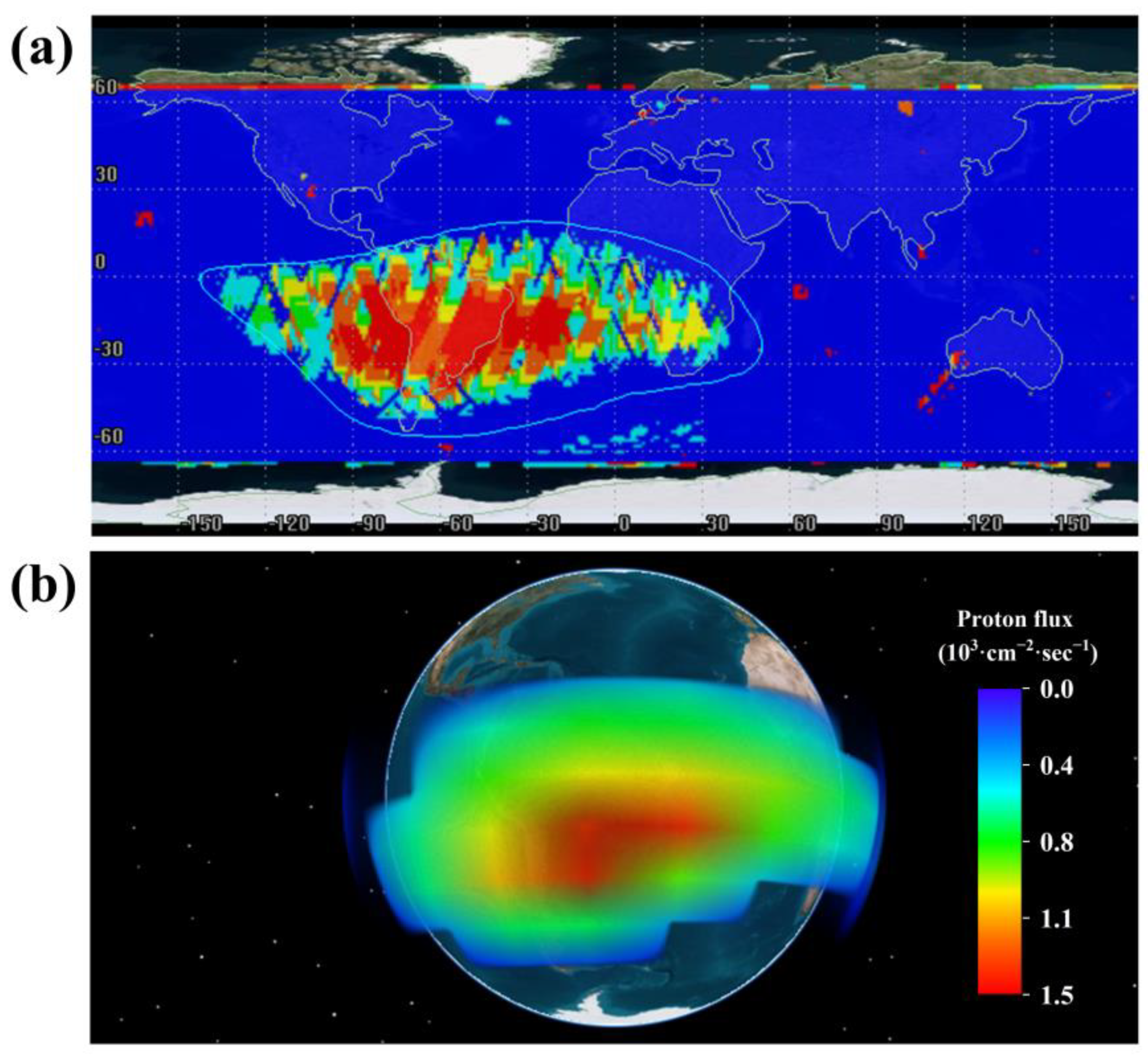
The data for Figure 8 were derived from proton flux data from all datasets, with Figure 8a representing the World map of proton flux, and Figure 8b representing the 3D-View of proton flux. The plotting of Figure 8 is based on proton flux data detected by the satellite as it passes through certain points. Through Figure 8, we can observe the spatiotemporal distribution characteristics of proton flux throughout the satellite’s entire operational period. We observed a concentrated burst of proton flux within the SAA region, while proton flux in other regions remains relatively stable. This observation aligns closely with our previous analysis of the spatiotemporal distribution of proton flux.

Building upon these findings, we have incorporated latitude and longitude features into our future proton flux predictions. Additionally, we have introduced the Temporal Pattern Attention (TPA) mechanism, focusing specifically on the impact of the SAA region. This approach aims to enhance the accuracy and reliability of proton flux profile forecasting.

3.3. Construction and Optimization of TPA-LSTM Neural Network

The hybrid neural network architecture of this study, as illustrated in Figure 9, follows a sequential arrangement: data input layer, LSTM layer, TPA layer, dropout layer, LSTM layer, and output layer. The data input layer takes longitude, latitude, and proton flux feature values as inputs into the network. The first LSTM layer captures temporal dependencies in the time series data, handling the time series data of proton flux feature values. Following the LSTM layer, the TPA layer is introduced and applied to the proton flux feature values. A dropout layer is added after the TPA layer to prevent overfitting. The second LSTM layer enhances the prediction accuracy of proton flux. Finally, an output layer is set up to perform predictions on the proton flux feature values.

In this neural network model, longitude and latitude feature values serve as additional inputs, providing extra contextual information within the LSTM layer. This aids the model in better comprehending time series data and enhancing predictive performance. Specifically, when longitude and latitude fall within the SAA range, the model focuses more on the predictive outcome for that period. Proton flux, serving as the primary feature input, furnishes the core data information to the model. It directly participates in predicting proton flux, thereby achieving more precise predictive outcomes.

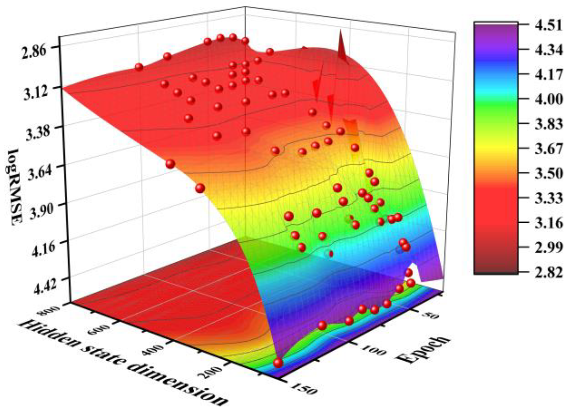
In the TPA-LSTM neural network model we employed, there are two crucial hyperparameters: hidden state dimensions and epochs. Properly configuring the number of hidden neurons can not only enhance predictive accuracy but also effectively prevent overfitting. To determine the appropriate hidden state dimensions, during the experimentation process, we initially utilized an empirical formula to obtain a rough range. The empirical formula is as follows:

$$N_h=N_s/(\alpha \ast (N_i+N_o\left)\right)$$

(16)

where $N_s$ is the number of samples in the training set, $N_i$ is the hidden state dimension of the input layer, $N_o$ is the hidden state dimension of the output layer, and $\alpha$ is an arbitrary value variable that can be taken by itself, usually 2–10.

For our neural network model, the training dataset size for each case was approximately 80,000 samples, while the hidden state dimensions for both the input and output layers were set to 16. Through calculations, we determined that the approximate range for the hidden state dimensions should be between 250 and 1200. During the tuning process, we experimented within this range to obtain the optimal hidden state dimensions.

The number of epochs, as one of the hyperparameters, also has a significant impact on the predictive results of the neural network. Insufficient epochs can lead to the underfitting of the model, while too many epochs can result in overfitting.

Figure 10 illustrates the impact of hidden state dimensions and epochs on the logRMSE value. With 40 epochs and a hidden state dimension of 800, the predicted logRMSE value reaches 3.00. This set of hyperparameters strikes a suitable balance between prediction accuracy and computational cost.

3.4. Experiments and Analysis

Figure 11 depicts a comparison of proton flux predictions among the TPA-LSTM model and the AP-8 model (model version: solar maximum, threshold flux for exposure: 1 cm²/s). The AP-8 model is primarily used to describe electron and proton fluxes between low Earth orbit (LEO) and the Earth’s atmosphere. It provides important parameters for characterizing these particle flows, such as flux and energy spectrum distribution [25]. 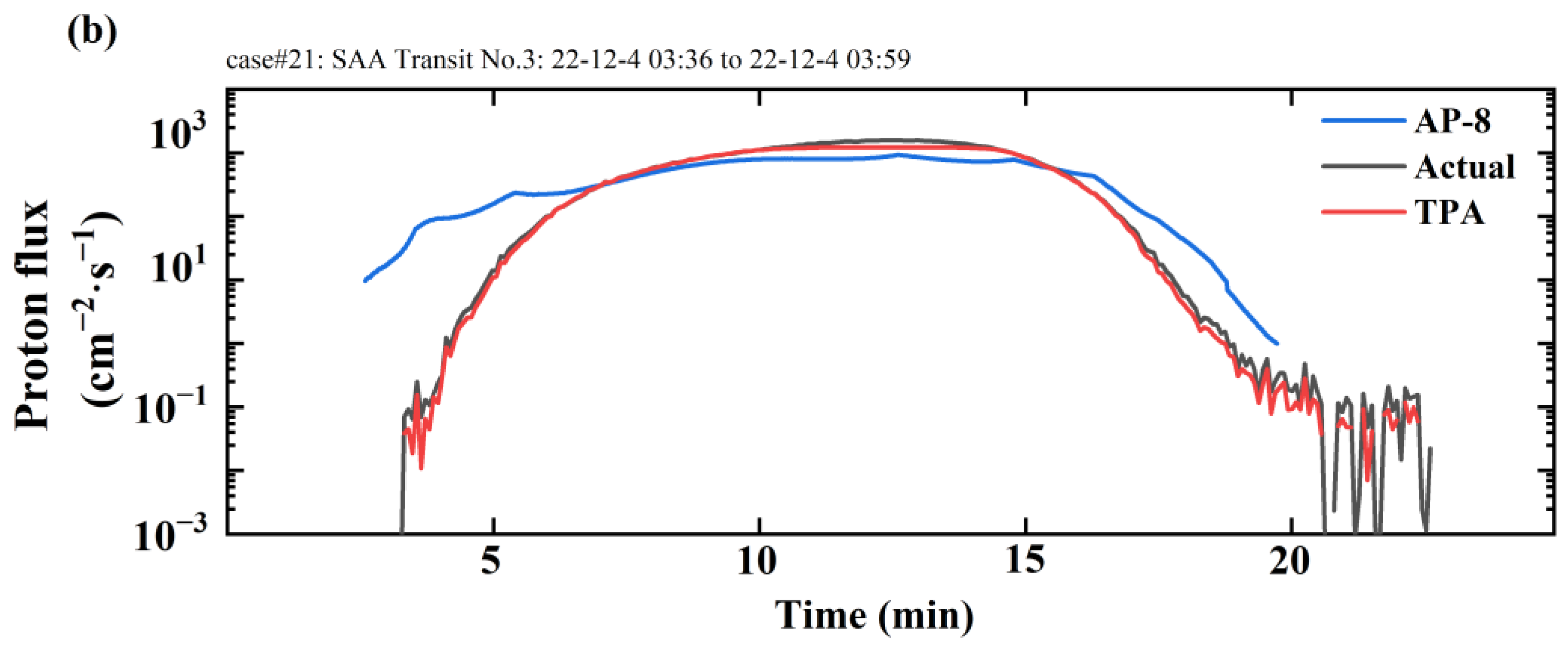Figure 11a represents the prediction scenario for case#21, which includes 16 peaks, each of them caused by the satellite transiting the SAA region. Appendix A 

Table A2. SAA transit times of case#21.

No.	Entrance Time	Exit Time	Duration (min)
1	2022/12/04 00:04	2022/12/04 00:24	19.6
2	2022/12/04 01:49	2022/12/04 02:11	21.6
3	2022/12/04 03:36	2022/12/04 03:59	22.4
4	2022/12/04 05:24	2022/12/04 05:46	22.1
5	2022/12/04 07:10	2022/12/04 07:32	22.3
6	2022/12/04 07:55	2022/12/04 07:59	3.2
7	2022/12/04 08:54	2022/12/04 09:08	13.1
8	2022/12/04 09:39	2022/12/04 09:51	11.9
9	2022/12/04 10:39	2022/12/04 10:46	6.8
10	2022/12/04 11:20	2022/12/04 11:40	19.4
11	2022/12/04 13:04	2022/12/04 13:27	22.9
12	2022/12/04 14:50	2022/12/04 15:13	22.1
13	2022/12/04 16:39	2022/12/04 16:56	16.4
14	2022/12/04 18:31	2022/12/04 18:40	8.9
15	2022/12/04 20:21	2022/12/04 20:25	3.4
16	2022/12/04 21:13	2022/12/04 21:26	13.0
17	2022/12/04 22:56	2022/12/04 23:15	18.4

provides detailed information on the satellite transits through the SAA region, including the entrance time, exit time, and duration of each crossing. Figure 11b depicts the prediction scenario for the third peak within Figure 11a.

To mitigate the influence of prediction randomness, we conducted a minimum of 50 runs for each model across various scenarios, and the average logRMSE and logMAE values are listed in

Table 3. Evaluation criteria of prediction results of different models.

Metrics/Model	TPA-LSTM	AP-8
logRMSE	3.71	4.19
logMAE	2.25	3.26

. From the results listed in Table 3, the following conclusions can be drawn: All two models exhibit commendable performance, with the TPA-LSTM model demonstrating the highest proficiency, achieving a logRMSE of 3.71. Notably, the TPA-LSTM model outperforms the AP-8 model in terms of predictive accuracy, boasting an approximately 2.03 higher logRMSE compared to the AP-8 model.

When focusing on the South Atlantic Anomaly (SAA) region, the predictive performance of the AP-8 model experiences a decline, while the TPA-LSTM model’s predictive performance is enhanced. As shown in

Table 4. Evaluation criteria of prediction results of different models in SAA.

Metrics/Model	TPA-LSTM	AP-8
logRMSE	3.09	5.74
logMAE	1.12	5.30

, the TPA-LSTM model’s logRMSE value decreases by 0.62, and the logMAE value decreases by 1.13 in the SAA region. The TPA-LSTM model demonstrates good predictive capability for proton flux in the SAA region, meeting the expected performance criteria. However, the AP-8 model exhibits poorer predictive performance in the SAA region. Its logRMSE value increases by 1.55, reaching 4.19, and its logMAE value increases by 2.04. This predictive performance falls short of our requirements for proton flux forecasting. The application of TPA distinguishes our model from the AP-8 model, and our model exhibits enhanced predictive performance in the South Atlantic Anomaly (SAA) region.

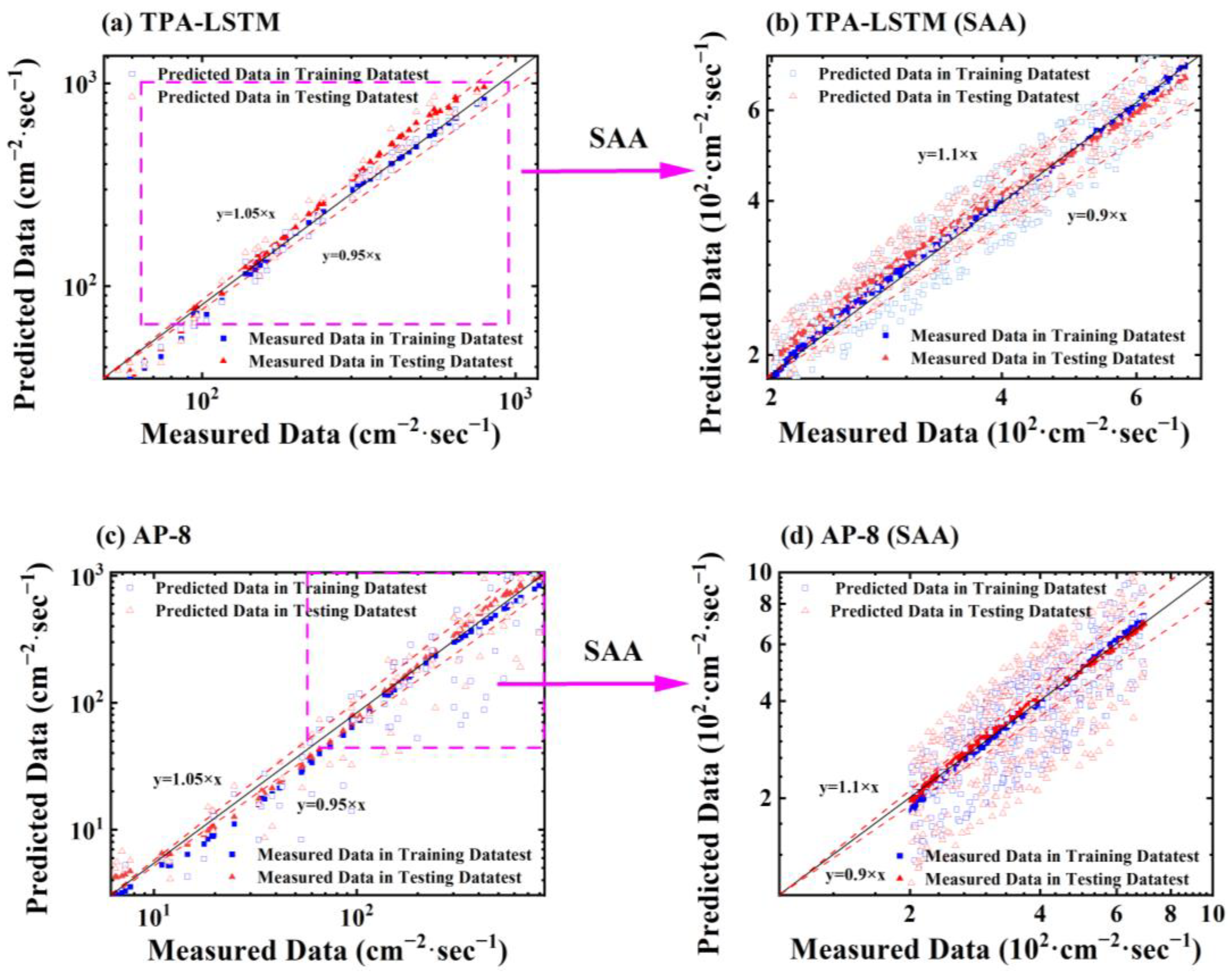
Figure 12 presents scatter plots of predicted values versus actual values for 26 cases for both the TPA-LSTM model and the AP-8 model. Figure 12a,c show scatter plots of predicted versus actual values for the entire time series for the TPA-LSTM model and AP-8 model, respectively, with the red line indicating a 5% error range. Figure 12b,d depict scatter plots of predicted versus actual values for the SAA region for the TPA-LSTM model and AP-8 model, respectively, with the red line indicating a 10% error range. By comparing the two models, we can clearly see that the data points from the TPA-LSTM model are more tightly distributed within the confidence region, both for the entire time series and within the SAA region. These two confidence regions encompass the majority of data points, showcasing how our predictive model accurately captures the variations in proton flux in the vast majority of cases. By examining Figure 12a, we can further observe that in regions with low proton flux intensity (typically, low-intensity proton flux is mostly found in non-SAA regions), the distribution of predicted points is more scattered. Conversely, in regions with high proton flux intensity, the distribution of predicted points is more clustered. This further validates our model’s grasp of spatial characteristics, leading to better predictive performance in the SAA region. Although a few data points lie outside the confidence region, overall, our predictive outcomes exhibit a high level of accuracy across the entire time series.

Additionally, in the error distribution plot within the SAA region, we can observe that the data points are more scattered compared to the entire time series. However, the majority of data points from the TPA-LSTM model still fall within the confidence region, indicating that our predictive model maintains a high level of accuracy even within this challenging zone. However, we acknowledge the greater challenge posed by predicting within the SAA region. Hence, in our future research, a heightened focus on optimizing predictions within the SAA region will be imperative to further enhance the model’s performance in this critical area.

In general, the results obtained through multiple runs and averaging indicate that the TPA-LSTM model demonstrates a high level of stability and accuracy in predicting proton flux. This model utilizes the TPA mechanism and LSTM architecture to capture the time- dependence of proton flux profiles measured during satellite operation more comprehensively and with heightened sensitivity, particularly within the SAA region. This sensitivity proves beneficial for enhancing the precision of proton flux predictions. However, it is important to note that forecasting within the SAA region remains a challenging task, necessitating further refinement and optimization to meet higher predictive demands.

4. Conclusions

This paper explores the use of a novel hybrid neural network model named TPA-LSTM for predicting proton flux profiles along a specific satellite orbit mentioned in the article. We applied the moving average wavelet transform method to preprocess the proton flux data. Subsequently, leveraging insights from the analysis of proton flux data, we introduced latitude and longitude features, along with the TPA attention mechanism, to enhance the focus on proton flux variations within the South Atlantic Anomaly (SAA) region. Finally, the TPA-LSTM hybrid neural network model was designed and trained and validated using proton flux data during the operational period of the specified satellite orbit. This model demonstrates higher accuracy in predicting proton flux compared to the AP-8 model. The key findings of this study are as follows:

• The moving average wavelet transform method demonstrates effective data preprocessing performance, proficiently retaining trend information while also effectively denoising the original dataset.
• The hybrid neural network model presented in this paper demonstrates a high level of predictive performance, with an average logRMSE of 3.4. Even in the case of the lowest predictive performance, the logRMSE still reaches 3.71.
• The neural network model, enhanced with latitude and longitude features and the TPA mechanism, demonstrates improved accuracy in capturing crucial time intervals influenced by latitude and longitude features within the SAA region. This enhancement effectively boosts the predictive performance of proton flux, with an average logRMSE of 3.09 for the SAA region.

Hence, the TPA-LSTM neural network model demonstrates a high level of accuracy in the field of predicting radiation proton flux. The implementation of the TPA attention mechanism allows for the comprehensive utilization of spatiotemporal features. Our approach can provide valuable assistance in space science research, such as the prediction of solar proton events. However, it is important to note that predicting space weather events requires not only a focus on particle flux data but also on features such as solar activity, magnetic field status, and more, and this is one of our future research directions.