Abstract
In this research, we introduce a deep-learning-based framework designed for the prediction of transonic flow through a linear cascade utilizing large-scale point-cloud data. In our experimental cases, the predictions demonstrate a nearly four-fold speed improvement compared to traditional CFD calculations while maintaining a commendable level of accuracy. Taking advantage of a multilayer graph structure, the framework can extract both global and local information from the cascade flow field simultaneously and present prediction over unstructured data. In line with the results obtained from the test datasets, we conducted an in-depth analysis of the geometric attributes of the cascades reconstructed using our framework, considering adjustments made to the geometric information of the point cloud. We fine-tuned the input using 1603 data points and quantified the contribution of each point. The outcomes reveal that variations in the suction side of the cascade have a significantly more substantial influence on the field results compared to the pressure side and explain the way graph neural networks work for cascade flow-field prediction, enhancing the comprehension of graph-based flow-field prediction among developers and proves the potential of graph neural networks in flow-field prediction on large-scale point clouds and design.
1. Introduction
For engine-fan cascades, localized complex flows in the flow field, such as shocks and wake, are the main sources of fan aerodynamic losses [1,2,3,4]. Studies [5,6] have shown that, especially in transonic and supersonic flow regimes, there is a significant increase in losses, with shock losses dominating the overall losses in the linear cascade. Inadequate design can lead to the generation of shocks and shock wave/boundary layer interaction [7], consequently resulting in energy dissipation and decreased efficiency. Wake losses also constitute a principal contributor to losses in transonic blades [8,9]. Concurrently, wake exerts an influence on the flow field within the downstream blade row passage [3], therefore impacting the aerodynamic performance of the fan. Thus, a fine design of the cascade profile is required to improve the fan efficiency. During the design process, deep learning is commonly used to construct surrogate models to quickly predict the flow field [10,11], while exploring the relationship between cascade geometry and flow losses can guide the design. Therefore, the development of a framework that allows for an in-depth understanding of flow-field characterization and flow-field prediction results can serve well both to fulfill the design process requirements for fast, low-cost flow-field prediction and to further guide subsequent design.
Multiple methods have been proposed for fast flow-field prediction, of which convolutional neural network (CNN) is frequently employed in the prediction of flow around airfoil profiles due to the potent nonlinear mapping [12,13,14] and feature extraction [15,16,17,18] capabilities. Sekar et al. [19] performed training on a set of airfoils based on deep CNN and deep Multilayer Perceptron, where CNN was employed for parameterization, while a deep MLP network was used to predict the flow field around the airfoil, achieving great prediction accuracy in flow field prediction. The research demonstrated the excellent feature extraction capabilities of CNN, which effectively extracted airfoil features and fitted the airfoil. Meanwhile, the use of the deep MLP network avoided the decrease in accuracy in fitting the airfoil boundary in traditional image-to-image-regression scenarios. Hui et al. [20] developed a CNN-based model to predict the pressure distribution over an airfoil. The proposed model achieved a mean squared error of less than 2% for test cases. Wu et al. [21] proposed a CNN-DCNN model, tested the influence of training parameters, and quantified the feature extraction capabilities of the presented model. Despite CNN demonstrating excellent predictive performance, precision, and the ability to capture inherent flow characteristics, particularly in the context of airfoil flow-field prediction, the capability of CNN in handling unstructured flow-field data remains suboptimal, particularly in practical applications with irregular flow path structure [22,23].
Due to the intricate flow patterns around three-dimensional turbine blades, researchers have introduced linear cascade testing to approximate blade performance, which extracts a specific cross-sectional blade profile from an overall blade and unfolds the profile circumferentially to create a linear structure [24]. Within the linear structure, profiles are arranged linearly to simulate the motion of annular blades in the flow field. For numerical simulations of airfoils, the equations are typically solved over the entire surface of the airfoil. In contrast, numerical simulations for flow over cascades are often conducted within one single flow path of the linear cascade, as illustrated in Figure 1, where the upper boundary in numerical simulation corresponds to the pressure side of the cascade, and the lower boundary corresponds to the suction side, forming a linear cascade through periodic configuration. Standard 2D-image-to-2D image-regression scenarios based on CNN commonly handle images in the regular shape of (height, width, depth), as the filters are fixed. However, for the irregular flow field depicted in Figure 1, conventional CNN-based methods may not be well-suited, as ordinary CNN approaches are constrained in generalizing to unstructured data because of the challenge of selecting a fixed convolution kernel that can effectively accommodate the various grid sizes, shapes, and irregular boundaries.

Figure 1.
Linear cascade single flow path schematic diagram.
Graph Convolutional Network (GCN) can directly extract spatial features from topological graphs, showcasing superior adaptability and flexibility in swiftly generating flow fields, especially for flow over irregular geometries. Figure 2 illustrates the transonic cascade Mach number field employed in this paper for flow-field prediction, in which the grid-based model outperforms the CNN-based model, which is limited to pixelation at a globally consistent resolution, in identifying details in the flow field over the cascade. It also indicates that, in the case of transonic cascades, the complex flow patterns and irregular flow path structure may result in the loss of crucial flow-field information in CNN-based field prediction.
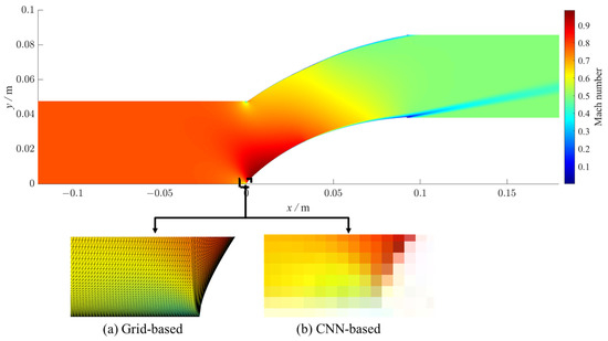
Figure 2.
Identifications of the details in the flow field over the cascade based on different models.
Moreover, GCN effectively captures both topological structures [25] and flow features [26]. Additionally, GCN leverages sparse matrices for computation, enabling the handling of larger matrices and accommodating extensive discrete flow-field points. Meanwhile, convolutional networks aggregate features from neighboring nodes, optimizing the utilization of topological information between these nodes [27]. Consequently, GCN finds application in the realm of flow-field reconstruction. Economon et al. [28] combined traditional GCN with CFD simulations, which significantly accelerated prediction speed. To address non-Euclidean flow problems, Wang et al. [29] integrated GCN with traditional numerical solvers and proposed the FlowGCN solver, which significantly speeded up the convergence of the entire program and secured accurate predictions. Peng et al. [26] proposed a data-driven flow prediction framework, GraphSAGE, based on the basic architecture of GCN. This framework learned potential features by sampling and aggregating features from the local neighborhoods of vertices, demonstrating good adaptability to non-uniformly distributed grid data. Furthermore, taking advantage of the use of sparse matrices in graph neural networks, GCN can effectively process and predict large-scale flow fields. Strönisch et al. [30] found out that GCN could predict flow fields over NACA airfoils and handle a large number of flow-field data points, which benefited the computational runtime by providing initial flow distributions for CFD. However, current research mainly focuses on cases such as airfoil and cylinder flow, with less emphasis on studies related to turbine blade cascades. Given that transonic/supersonic blade cascade flow fields are more complex and involve shock waves, multiple flow interactions [31,32], resulting in spatial non-uniformity and temporal non-stationarity in the flow field, it is essential to establish a prediction framework with higher-resolution flow-field data to improve predictions of the characteristics of turbine blade cascade flow.
Furthermore, despite the significant progress made by GCN in predicting fluid fields, there is still a need for further research on elucidating how GCN predicts these fluid fields. Presently, various methods for interpreting graph neural networks (GNNs) have been developed. Ying et al. [33] analyzed the impact of node features and the linking process of node information aggregation on model predictions and proposed GNNExplainer, which identified crucial subgraph structures and node features within GNN predictions, demonstrating a general and model-agnostic property. SubgraphX [34] focused on the substructures of the graph, interpreting GNN by exploring and identifying significant subgraphs. GNN Prediction Interpreter (GPI) [35] studied the correlation between node features and GNN predictions and elucidated the impact of node features on GNN predictions. Although explanations for graph neural networks have primarily focused on important subgraph structures and node features [27,36,37], explanations for fluid field regression tasks are yet to be fully developed.
Currently, some studies represent the flow field with geometric points and aerodynamic information [38], effectively avoiding the impact of pixelation on data accuracy and the high costs associated with increasing flow-field resolution [22]. Kashefi et al. [39] proposed a novel deep-learning framework for predicting steady incompressible flow on multiple sets of irregular geometries based on PointNet and tested the effectiveness of the PIPN in the case of incompressible flows and thermal fields. To reduce the computational cost of numerical simulations, Xiong et al. [40] designed a point-cloud deep neural network based on the PointNet architecture and established a mapping between the spatial position of the ONERA M6 wing and CFD calculation values to predict the aerodynamic characteristics of the three-dimensional geometry. The results indicate that the computational cost can be reduced by approximately 23% under comparable predictive accuracy. However, while existing point-cloud-based techniques have been evaluated in many flow scenarios, little study has been done on engine flow fields.
Based on the aforementioned research, this work constructs prediction models in the form of graphs based on GCN since CNN primarily collects characteristics from two-dimensional images, whereas the data structures of cascade flow fields are often more complicated. Grid resolution should be enhanced to capture flow features in blade cascades. This method allows for the prediction of flow fields on large-scale, non-uniform grids while maintaining the benefits of feature extraction. We deliver a point-cloud and GCN-based deep-learning architecture in this research. This framework aims to predict the turbulent viscosity and pressure fields around the fan cascade flow. It employs the model based on GCN to extract geometric information and deliver aerodynamic information at different positions in the flow field from point-cloud inputs with up to 295,035 points. This work first generates 1000 distinct cascade samples with varying disturbances, using the Hicks–Henne parameterization approach, which are then subjected to CFD simulations and data processing to generate point-cloud data as the dataset. Model parameters based on GCN are adjusted to provide predictions for the pressure and turbulent viscosity fields. Subsequently, we conducted an in-depth analysis of the specific understanding mechanism of the model based on graph encoding methods concerning the flow field. The key characteristics of this work are as follows:
- A novel framework has been devised to predict flow fields over the cascade, combining GCN with point clouds to enhance prediction accuracy;
- This innovative framework facilitates swift and precise predictions across an extensive grid containing 295,035 flow-field points, ensuring large-scale flow-field analysis efficiency;
- A detailed investigation has been conducted to unravel the underlying mechanisms of GCN in the context of flow-field prediction, shedding light on its intricate understanding and application.
The paper is structured as follows: Section 2 explains the cascade geometry generation and numerical simulation, Section 3 introduces the structure of the framework and implementation of deep learning, Section 4 presents the results, followed by a discussion of the findings and limitations of the current approach in Section 5, while Section 6 provides the conclusions.
2. Numerical Methods and Dataset Generation
2.1. Cascade Geometry Generation
The subject in the research is a specific type of linear cascade profile. In this study, the Hicks–Henne bump function is applied as the parameterization method, through which the linear superposition of the perturbation function and the midrib analytic function characterize the cascade profile. The expression for this function is:
where and stands for the suction side and pressure side of the cascade; and represents the y-coordinates on the suction and pressure sides of the original cascade; x represents the location of the mean aerodynamic chord, which ranges from 0 to 1; i stands for the sequence number of the design variable; n represents the number of the shape function; stands for the weight of the i-th shape function, which determines the thickness distribution. is the shape function, which can be expressed as:
where w represents the width of the bump; and stands for the location of the bump.
In this paper, the perturbation on the suction and pressure sides of the cascade is generated based on the Hicks–Henne function. Three perturbation points on each surface are positioned at relative chord lengths of 0.05, 0.4, and 0.7, with mean values corresponding to the original profile data at these relative chord positions and a variance of 0.0577. To ensure a uniform distribution of geometric parameter samples, the Latin Hypercube Sampling (LHS) method is employed for selecting specific parameter values. Moreover, a constraint has been enforced to guarantee that the thickness variations at each profile point do not surpass 10% of the initial thickness. This constraint has led to the creation of 1000 profile shapes, as depicted in Figure 3.
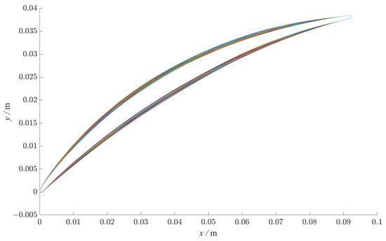
Figure 3.
The geometry of the 1000 generated cascades.
2.2. CFD Simulation and Dataset Generation
For the generated 1000 geometric shapes, the computational domain is divided as shown in Figure 4, which calculates a single flow channel of the periodic flow field with a Reynolds number of approximately 1.9 × 10⁶. The grid over the blade surface is controlled as y+ ≈ 1/2, with the size on the order of 10−6 m. Over the surface of the cascade, 1603 grid points are set, and the far-field length is nearly four times the length of the cascade.

Figure 4.
Grids of outline and magnified details at dense grids.
As illustrated in Figure 1, the flow channel is divided into three parts: the leading-edge inlet channel, the cascade passage, and the trailing-edge outlet channel. The lengths of the inlet and outlet channels are each extended by 1 chord length beyond the leading and trailing edges of the profile. For the leading-edge inlet and outlet channels, periodic boundary conditions are applied to the upper and lower parts. Inlet and outlet boundaries are set as pressure boundaries, with inlet total pressure of 119,950 Pa, total inlet temperature of 293 K, outlet static pressure of 101,325 Pa, total temperature of 293 K, turbulence intensity of 0.2%, and turbulent viscosity ratio of 10. The no-slip boundary condition is set at the surface.
During the simulation, Reynolds-Averaged Navier–Stokes (RANS) and the transition SST four-equation model [41] are selected. RANS equations can be described as:
Additionally, an implicit solution and the second-order upwind scheme for the solution format are chosen. Grid independence verification is conducted, and the numerical results are presented in Table 1, which demonstrates that when the total number of grids increases to 170 K, the relative change rate of the total pressure loss coefficient η and the inlet static pressure Pst decreases to within 0.4%, meeting the grid independence requirements. To accurately predict the cascade flow field based on GCN, a grid number of 295,035 is ultimately selected for the subsequent optimization database construction, as the results are basically unchanged with the increase of the grid numbers.

Table 1.
Grid Independence of the linear cascade.
Numerical simulations are performed over 1000 generated cases to generate an array containing flow-field information, including the coordinates of each grid vertices, along with corresponding static pressure and turbulent viscosity, stored in the form of point clouds. Each case consists of a point cloud of size 295,035. The dataset split ratio for training, testing, and validation sets is 8:1:1.
3. Deep-Learning GCN-Based Framework and Model Training
3.1. The Structure of the Framework
To process discrete data representations of the output flow field, they need to be transformed into graph form. A graph is defined as G = (V, E), where V represents the set of 295,035 nodes and E represents the set of edges. In this research, each node corresponds to a discrete grid point in the flow field, and the eigenvector comprises coordinates and aerodynamic parameters. Edges are formed by connecting points on the surface of the cascade with various grid points in the flow field and their relative relations. The generated graph comprises multiple subgraphs, with each subgraph depicted as illustrated in Figure 5. In this representation, node 0 represents the original nodes, the light brown nodes 1,2,3 represent the neighborhood, corresponding to the 3 spatial neighbors in the grids and 1603 points on the profile surface, and the green nodes 4,5,6,7,8 represent the indirect neighborhood. In addition, a global node containing the Mach number and the direction of the stream is added to the graph and fully connected with each node to guarantee the model generalization. The edge is defined as the relationship between the original node and its neighbors, with each node having a total of 1606 edges.

Figure 5.
The generation and the structure of the input graph of the model.
The pressure and turbulent viscosity values for each grid point in the flow field are calculated using weighted propagation based on the eigenvectors of each node. The message-passing scheme can be expressed mathematically as follows:
where h stands for the embedding of the nodes, v and u are the index of the node, N(v) is the neighbor nodes of node v, k represents the number of the layer, is the activation function, Wk and Bk stands for the calculating matrix, and AGG stands for the generalized aggregation function. In this study, aggregation and update functions can be expressed as:
Through the aggregation function, it becomes evident that the process considers not just the number of nodes adjacent to a given node but also the number of neighbors that those adjacent nodes have. The process involves computing a weighted sum of the target node and all its nearby nodes. This also indicates that GCN is effective in handling non-Euclidean discrete data from the flow field [42].
In the study, the point cloud is fed into the model displayed in Figure 6 after undergoing the preprocessing steps detailed above to create a graph. The pressure and turbulent viscosity properties of each node make up the output. In the particular process, 3 GCN layers are employed as previous research has demonstrated that stacking convolutional layers is advantageous for feature extraction in the model [43]. Moreover, a smoothing layer is added at the end to perform averaging on the output graph and create a continuous flow field [44]. ReLU activation is implemented after the first two convolutional layers. The loss function is then used to train the hyperparameters of the model using the output from the smoothing layer and the last convolutional layer.
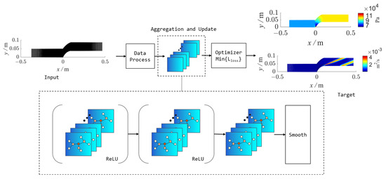
Figure 6.
The framework for the cascade flow-field prediction.
It has been proved that normalization helps speed up the convergence results [45]. Additionally, there is a significant difference in the magnitudes of the two output fields in the data structure presented in this paper, which may lead to the oscillation of the loss. As a result, each field, including the inputs and outputs, is normalized separately using the maximum-minimum scaling method.
3.2. Training
The choice of the loss function has a significant impact on the prediction results in regression problems [46], like flow-field prediction. In such cases, various loss functions, such as mean squared error (MSE), mean absolute error (MAE), Log-Cosh loss function, and Huber loss function, are commonly used. The research conducted separate tests on these four types of loss functions to compare their effectiveness. Training becomes unfeasible when gradient explosion problems arise from unstable convergence of loss functions defined by MSE. There is no discernible difference in the problem solution when the learning rate is changed. For turbulent viscosity field data, the difference between the wake area data and other sections is substantial, and since they are influenced by the data themselves, there may be a continual accumulation and amplification of prediction errors, resulting in gradient explosion. Analogously, there is a gradient issue during training and a notable oscillation issue during the convergence phase for the Log-Cosh loss function. When MAE is used as the loss function, the gradient is consistent for all prediction sites, and the convergence is sluggish. The consistent gradient problem can be avoided by dynamically modifying the learning rate to decrease with an increase in iteration. For the Huber loss function, of utmost importance is the adjustment of the hyperparameters δ, which can be written as:
When comparing different loss functions in machine learning models, the Huber loss function is more robust than MSE and faster in convergence than MAE as it reduces the gradient around the minimum value. After training and adjusting the hyperparameters with δ set to 1.35, Figure 7 displays the predicted results using MAE with dynamic learning rate and Huber loss function as loss functions, respectively. To display the prediction fields more clearly, a periodic operation is performed on the contours, which displays three flow channels simultaneously. The figure shows that the predicted results for the pressure field are satisfactory, while for the turbulent viscosity field, the predicted results using MAE as the loss function are significantly worse than those using the Huber loss function despite the application of dynamic decreasing learning rate. When dealing with high-turbulent-viscosity regions, the model based on the MAE loss function does not achieve the desired prediction effect and shows incomplete learning, while the model based on the Huber loss function has a stronger learning ability for these regions. Therefore, this article recommends using the Huber loss function for subsequent research, which is defined as Equation (9) with the variable of pressure and turbulent viscosity on each node.
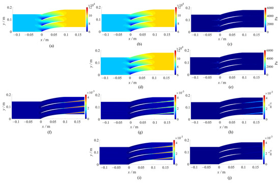
Figure 7.
Flow-field prediction based on the models utilizing MAE and Huber loss function as loss functions, respectively. (a,f) are the reference pressure field and turbulent viscosity field based on the CFD solution. (b,c,g,h) are the predicted flow fields and absolute error using MAE as the loss function. (d,e,i,j) are the predicted flow fields and absolute errors based on the Huber loss function.
Once the loss function has been determined, the hyperparameters of the batch of nodes, such as the learning rate, convolutional kernel size, and number of convolutional layers, should be adjusted. However, adjusting all parameters for large-scale learning of the entire flow field can be time-consuming. To address this issue, a grid search method can be used to construct a graph in the highly characteristic high-turbulent-viscosity region of the flow field shown in Figure 8, where incomplete learning occurs frequently and performs automatic hyperparameter tuning. In the grid search method, a grid containing all possible values is created for the selected adjusted parameters. Each iteration attempts its combination in a certain order and records the prediction performance, ultimately returning the model with the best performance. This article conducts a grid search on several parameter values such as learning rate, epoch, batch size, dropout rate, and the dimensionality of the output space and optimizer and chooses the hyperparameters with the highest prediction accuracy. Among the hyperparameters, the set can be expressed as follows: learning rate, epoch {100, 200, 500, 1000}, batch size {10, 50, 100, 500}, dropout rate {0.1, 0.2, 0.3, 0.4}, the dimensionality of the output space {64, 32, 16, 8, 4}, and optimizer {Adam, SGD}.

Figure 8.
The area where grid search works and the diagram of the grid search method.
After testing, the following hyperparameters yield the best performance: learning rate = 0.01, epoch =1000, batch size = 50, dropout rate = 0.2, the dimensionality of the output space = 16, 8, 2, respectively, and the optimizer chooses Adam. After the initial two convolutional layers, a ReLU activation function is added to improve the network’s ability to express nonlinear features and predict fields more accurately. Additionally, a smoothing layer is included after the last convolution layer to maintain the continuity of the flow field.
Training has been conducted on the dataset based on the determined hyperparameters and the model as described. Figure 9 illustrates the convergence of the model. After multiple epochs of training iterations, both the training and validation sets have tended to converge, indicating the effectiveness of the training. The convergence level of the validation set is also guaranteed to be within an acceptable range, which ensures that the trained model accurately predicts the flow field.
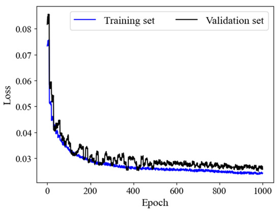
Figure 9.
The loss value for the model with the given hyperparameters on each epoch.
4. Results
4.1. Fields Prediction Performance
Different cases are considered to study the prediction results of the framework described in the second section, in which the leading-edge point of the cascade is located at the origin. The results are presented in the form of point clouds. To make the predicted results more comprehensible, contours are used to display the predicted pressure and turbulent viscosity fields. Figure 10 shows the flow-field prediction results, and Figure 11 presents the ratio of predicted values to CFD values for each point in the flow field, demonstrating their deviation from the y = x line. The figure indicates that the main structural and physical features in the flow field are successfully captured, while the areas with significant errors are mainly concentrated at the edges in pressure fields and high-turbulent-viscosity areas, which can be shown in Figure 11 that the predicted errors are concentrated in the low-pressure and high-turbulent-viscosity regions. In the pressure field, the pressure gradient at the leading edge of the cascade is much larger than that in the rest of the flow field, where the contour edges cannot be clearly displayed in the prediction and show larger errors in pressure field prediction, while the remaining parts exhibiting high prediction accuracy, including the high-pressure areas that appear at the suction side in certain cases. The low turbulent viscosity area on the surface of the cascade and the high-turbulent-viscosity feature at the trailing edge guarantee an accurate representation of the features of the cascade in the turbulent viscosity field prediction. Although predictions of the high-turbulent-viscosity region at the trailing edge and the prediction of the high-turbulent-viscosity region at the front edge are not adequate, both are still within an acceptable range, profiting from the combination of GCN and point cloud, which enables the framework to predict dominant regions under high resolution without increasing global resolution. Overall, the accuracy of the entire pressure field prediction is over 99%, while the turbulent viscosity field is more than 96%, as indicated in Figure 11, with the prediction speed of 87 s, converging four times faster than nearly 8 min in CFD.
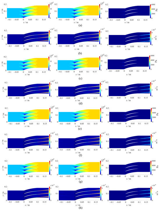
Figure 10.
Flow prediction based on a set model over different geometry. (a,c,e,g), respectively, display the CFD (left) and predicted pressure fields (middle), along with the absolute errors (right) for different geometries. (b,d,f,h), respectively, display the CFD (left) and predicted turbulent viscosity fields (middle), along with the absolute errors (right) for different geometries.
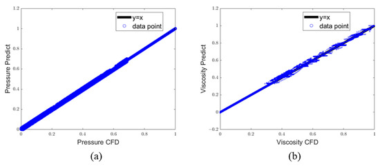
Figure 11.
Comparison of predicted fields and CFD fields value. (a,b) sequentially display the results of the pressure field and turbulent viscosity field.
An additional flow-field prediction model is CNN-based. To maintain a roughly consistent total number of points, the resolution of the flow-field images input to the CNN is set to 1000 × 500. The comparative results are illustrated in Figure 12. Due to resolution limitations, the CNN-based model exhibits poorer performance in identifying high-gradient boundaries within the flow field. In contrast, the GCN-based model is not affected by resolution constraints and can accurately predict pressure values in low-pressure regions. However, it shows suboptimal performance in predicting turbulent viscosity fields in regions with sparse nodes.
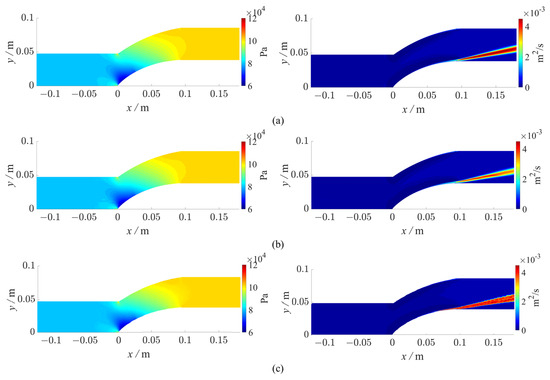
Figure 12.
Comparison of CFD fields, GCN-based predicted fields, and CNN-based predicted fields. (a–c) sequentially display the results of CFD, GCN-based model and CNN-based model.
4.2. Prediction of the Trained Model on Cascade with Different Nodes Selection Approach
In general, researchers interpret models by explaining the importance of specific indicators [47,48]. If the removal of a certain node significantly changes the prediction results, that node is considered important. To investigate which part of the cascade is more crucial in predicting cascade flow fields based on graph neural networks, global points are created for the 1603 points constituting the initial data cascade surface throughout the graph generation stage. This allows the framework to learn the characteristics of different flow channels. The flow field is projected, and the cascade surface points are rearranged. By removing different intervals of nodes, this process aims to analyze the features of the output flow field based on GCN predictions and understand the contribution of the cascade surface points to the flow field. As observed in the prediction results in Section 4.1, the predictions for the inlet and outlet of this flow field tend to converge, with a particular emphasis on the leading edge of the cascade and cascade wake. Consequently, additional research on the construction of the two regions, including information on 5797 and 1223 nodes sequentially, is conducted.
The selection of nodes is achieved by removing surface points with different intervals. To be specific, global nodes are removed from 1603 global points on the suction side and pressure side at intervals of 2 to 10, which sorts sequentially from the trailing edge to the leading edge. The predicted pressure and turbulent viscosity fields are compared with the originally predicted result in the regions of the cascade leading edge and the wake areas. For quantitative comparison, the new prediction values and the original values are weighted and take ratio, defined as contribution, which is expressed as:
where y is pressure or turbulent viscosity. The results are shown in Figure 13. After removing the intervals, the predicted pressure field at the leading edge remains the same as the original values. Meanwhile, there is no significant change in the predicted contribution values between the global points of each interval removed. The prediction results of global nodes removed at the same interval for the turbulent viscosity field in the wake region are shown in Figure 13b. Although there is a certain degree of change compared to the pressure field prediction as the interval increases, it is still minor. The study also investigated the effect of removing lower-order global points on the predicted flow field, which indicates that removing one or two nodes has almost no impact on the outcomes.
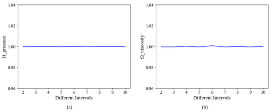
Figure 13.
The contribution based on prediction over the cascade leading edge and wake regions with different intervals of global nodes removed. (a,b) represents the results of the pressure and turbulent viscosity field, respectively.
The output of convolutional layers has been analyzed to learn additional information regarding the learning pattern of convolutional networks. In the selected area, the prediction over various starting locations of interval 10 is explored. The output ratios of the first and second convolution layers at various starting positions concerning the original convolution output are displayed in Figure 14. As per the results, removing nodes with the same interval but different starting points only causes slight changes in the prediction, as shown in Figure 14. The consistency of the findings remains nearly the same after the first layer of convolution output, demonstrating the GCN learning pattern on data processing in flow-field prediction. When the advertisement matrix and features are multiplied, the features of the nodes neighboring the certificate nodes are included, along with the aggregation of features over global nodes. As a result, the results provided in Figure 13 display a change interval without appreciable deviations from the anticipated outcomes.
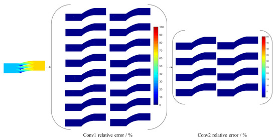
Figure 14.
The outcomes of the first and second convolution layers with different starting points.
4.3. Explanation of Graph Embedding Approach Based on the Framework
The convolution processing procedure on the flow-field data is displayed in Section 4.2. Further feature analysis is carried out on different parts with sequential 20, 50, 100, and 200 nodes removed, as shown in Figure 15, to investigate the impact of specific learning techniques of the GCN-based framework on the flow channel properties of cascades.
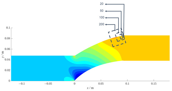
Figure 15.
Diagram of parts with 20, 50, 100, and 200 nodes.
Figure 16 illustrates the technique of the continuous 20, 50, 100, and 200 nodes on the cascade surface that affect the estimated pressure field in comparison to the initial predicted fields. As can be seen from Figure 15, points on the suction side have a considerable impact on the prediction results when consecutive nodes are excluded. On the other hand, the flow field is less affected by the pressure side channel properties that the trained model learns.
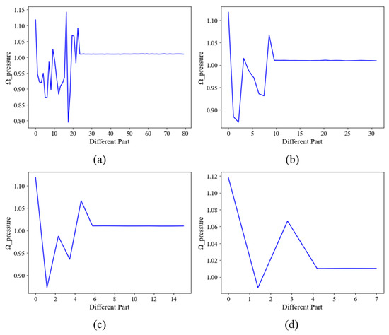
Figure 16.
The contribution based on prediction over the cascade leading edge with continuous steps of global nodes removed, where (a–d) represent the results with steps 20, 50, 100, and 200.
When the interval size is set to 10 instead of the corresponding step, a similar prediction trend is shown in Figure 17, indicating that the weight of nodes near the cascade surface learned by the framework to the prediction of the flow field is almost consistent.
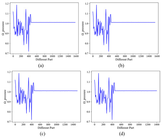
Figure 17.
The contribution shown in the same intervals based on prediction over the cascade leading edge with continuous steps of global nodes removed, where (a–d) represent the results with steps 20, 50, 100, and 200.
Figure 18 illustrates the impact of various cascade surface points on the wake region. In comparison to the suction side, the changes caused by the pressure side are much more subtle. The trailing edge of the suction side is most of the component contributing to the field, in which a substantially greater impact on the wake than the pressure field is observed. Additionally, it demonstrates agreement with the pressure field prediction for the prediction weights with the same interval.
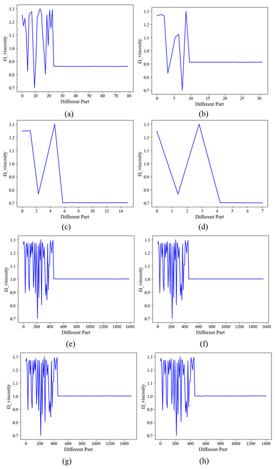
Figure 18.
The contribution based on prediction over the wake region with continuous steps of global nodes removed, where (a–d) represents the results with steps 20, 50, 100, and 200, while (e–h) stands for the plotting intervals of 10 with different steps.
5. Discussion and Limitations
The pressure and turbulent viscosity flow field along the cascade can be predicted with over 99% and 96% prediction accuracy with the proposed framework, respectively. The outcomes demonstrate that the framework is capable of handling large-scale point-cloud inputs and graph structures based on this, accurately capturing the characteristic structure of the fan cascade flow and predicting the pressure and wake turbulent viscosity regions at the leading edge of the cascade. According to the learning of partial flow fields in grid search and the final flow-field prediction results, the most distinctive portions of the flow field can be chosen for learning, negating the necessity to solve the full flow field as in CFD. Especially for engine flow situations, where the flow field shows more complexity, this framework is more flexible and does not require costly global resolution refinement due to partial flow characteristics.
Nevertheless, there are certain limitations of this framework for flow-field prediction as well, such as the relatively poor prediction precision for wave zones. The sparse grid in this area is most likely responsible for the inaccurate turbulent viscosity prediction, as the framework demonstrates an improved comprehension of features in the relatively dense part of the nodes, while surrounding nodes in the relatively sparse portion of the grid have relatively lower feature values, making it susceptible to the influence of neighboring nodes during the learning process. Simultaneously, additional investigation is required about the extrapolation of alternative operational conditions. It has been proven through learning that global nodes with smaller magnitudes do not substantially affect the outcomes of the trained model. Consequently, more research is required to confirm the efficacy of the global points defined in the framework, with the features of the Mach number and the inlet angle of attack.
The purpose of this study is to elucidate the mechanism of the flow path feature learning process utilizing the GCN-based framework. To accomplish the goal, nodes with various positional characteristics are removed from the graph, and the resulting variations in prediction outcomes are noted, serving as the foundation for the GCN explanation. The results gathered show that in the GCN-based model, learning global node features requires the feature addition of neighboring nodes. As a result, for fewer global node inputs with evenly distributed positional information, the model remains producing outputs with great precision. The nodes at the trailing edge of the cascade suction side have a substantial impact on the turbulent viscosity field prediction by the framework, as demonstrated by the findings of a study on the influence of global nodes with non-uniform distribution position features on flow-field prediction results. Despite having a negligible effect on the turbulent viscosity field, the suction side also influences the pressure field prediction to some extent. When predicting the turbulent viscosity field at a thickness of 10% and loading requirements for a certain cascade, the pressure side has a lesser influence, where the impact on the field prediction is negligible.
This study has exclusively focused on the investigation of 2D profiles, necessitating an extension to encompass the analysis of blades. Meanwhile, the existing data are derived from solving RANS equations. For future investigations, higher precision data will be pursued through the implementation of more advanced techniques such as large eddy simulation (LES) or direct numerical simulation (DNS). Additionally, in the computational setup of this paper, including a subgraph to reconsider the effects of the neighboring nodes will lead to an increase in computational costs. Utilizing graph summarization methods, such as graph compression or graph feature extraction (e.g., using techniques like autoencoders), during the preprocessing stage may effectively reduce computational costs [49], which compresses large-scale graph data into a more concise form, reducing redundancy and enabling a more effective analysis and understanding of large-scale graph data.
6. Conclusions
Our study proposes a deep-learning framework that utilizes point clouds and GCN to accurately predict the flow field of cascades. The method involves converting CFD grid data into point-cloud data and the detailed data conversion method of feeding the point cloud into a GCN-based model, as well as fine-tuning the network hyperparameters and training process. Utilizing the framework, we can predict the flow field and employ the trained model to help explain the GCN interpretation of the cascade flow field, thus enhancing the understanding of the flow-field features.
Based on the results gathered, the proposed framework is capable of effectively predicting the flow situation in the cascade, establishing a mapping of flow-field position information and aerodynamic information, and efficiently processing large-scale point-cloud data. Meanwhile, it provides valuable data support for learning local flow characteristics instead of solving the entire flow field as in CFD simulations. For the given graph as the input of the model, results suggest that the trailing-edge point of the cascade is the crucial part that significantly impacts the important feature points of the cascade, which should be considered to be important input global nodes.
In addition, the loss function and hyperparameters of the framework are also tested. The outcomes suggest that the selection of loss function significantly affects the convergence of flow-field prediction. It is still necessary to enhance the generalization capacity of the existing loss function, which does not incorporate the constraints of the N-S equation. The introduction of the physics-informed neural network (PINN) may improve the model performance and effectively utilize the gradient information in graph neural network calculations [50,51,52]. In the future, the prediction and generalization performance of the model will be further improved by introducing N-S equation constraints, thus improving the interpretability of the model, and optimizing design will be developed based on the learned cascade flow channel characteristics.
Author Contributions
Conceptualization, G.S., J.F. and M.Z.; Methodology, G.S., X.L. and L.W.; Software, X.L. and C.W.; Validation, X.L.; Formal Analysis, X.L. and L.W.; Investigation, X.L.; Resources, G.S. and X.L.; Data Curation, X.L.; Writing – Original Draft Preparation, X.L. and L.W.; Writing—Review & Editing, G.S., X.L., L.W., C.W., J.F. and M.Z. All authors have read and agreed to the published version of the manuscript.
Funding
This research received no external funding.
Data Availability Statement
The data presented in this study are available on request from the corresponding author.
Conflicts of Interest
The authors declare no conflict of interest.
References
- Bloch, G.S.; Copenhaver, W.W.; O’Brien, W.F. A Shock Loss Model for Supersonic Compressor Cascades. J. Turbomach. 1999, 121, 28–35. [Google Scholar] [CrossRef]
- Kusters, B.; Schreiber, H. Compressor cascade flow with strong shock-wave/boundary-layer interaction. AIAA J. 1998, 36, 2072–2078. [Google Scholar] [CrossRef]
- Lengani, D.; Simoni, D.; Ubaldi, M.; Zunino, P.; Bertini, F.; Michelassi, V. Accurate Estimation of Profile Losses and Analysis of Loss Generation Mechanisms in a Turbine Cascade. J. Turbomach. 2017, 139, 121007. [Google Scholar] [CrossRef]
- Hammer, F.; Sandham, N.D.; Sandberg, R.D. The Influence of Different Wake Profiles on Losses in a Low Pressure Turbine Cascade. Int. J. Turbomach. Propuls. Power 2018, 3, 10. [Google Scholar] [CrossRef]
- Li, S.-M.; Chu, T.-L.; Yoo, Y.-S.; Ng, W.F. Transonic and Low Supersonic Flow Losses of Two Steam Turbine Blades at Large Incidences. J. Fluids Eng. 2005, 126, 966–975. [Google Scholar] [CrossRef]
- Wang, Z.; Chang, J.; Li, Y.; Kong, C. Investigation of shock wave control by suction in a supersonic cascade. Aerosp. Sci. Technol. 2021, 108, 106382. [Google Scholar] [CrossRef]
- Schreiber, H.A.; Starken, H. An Investigation of a Strong Shock-Wave Turbulent Boundary Layer Interaction in a Supersonic Compressor Cascade. J. Turbomach. 1992, 114, 494–503. [Google Scholar] [CrossRef]
- Xu, L.; Denton, J.D. The Base Pressure and Loss of a Family of Four Turbine Blades. J. Turbomach. 1988, 110, 9–17. [Google Scholar] [CrossRef]
- Denton, J.D.; Xu, L. The Trailing Edge Loss of Transonic Turbine Blades. J. Turbomach. 1990, 112, 277–285. [Google Scholar] [CrossRef]
- Wu, H.; Liu, X.; An, W.; Chen, S.; Lyu, H. A deep learning approach for efficiently and accurately evaluating the flow field of supercritical airfoils. Comput. Fluids 2020, 198, 104393. [Google Scholar] [CrossRef]
- Rabault, J.; Ren, F.; Zhang, W.; Tang, H.; Xu, H. Deep reinforcement learning in fluid mechanics: A promising method for both active flow control and shape optimization. J. Hydrodyn. 2020, 32, 234–246. [Google Scholar] [CrossRef]
- Murata, T.; Fukami, K.; Fukagata, K. Nonlinear mode decomposition with convolutional neural networks for fluid dynamics. J. Fluid Mech. 2020, 882, A13. [Google Scholar] [CrossRef]
- Fukami, K.; Nakamura, T.; Fukagata, K. Convolutional neural network based hierarchical autoencoder for nonlinear mode decomposition of fluid field data. Phys. Fluids 2020, 32, 095110. [Google Scholar] [CrossRef]
- Han, R.; Wang, Y.; Zhang, Y.; Chen, G. A novel spatial-temporal prediction method for unsteady wake flows based on hybrid deep neural network. Phys. Fluids 2019, 31, 127101. [Google Scholar] [CrossRef]
- Chen, T.; Chu, Q.; Tan, Z.; Liu, B.; Yu, N. BAUENet: Boundary-Aware Uncertainty Enhanced Network for Infrared Small Target Detection. In Proceedings of the ICASSP 2023–2023 IEEE International Conference on Acoustics, Speech and Signal Processing (ICASSP), Rhodes Island, Greece, 4–10 June 2023; pp. 1–5. [Google Scholar]
- Berenjkoub, M.; Chen, G.; Günther, T. Vortex boundary identification using convolutional neural network. In Proceedings of the 2020 IEEE Visualization Conference (VIS), Virtual, 25–30 October 2020; pp. 261–265. [Google Scholar]
- Jogin, M.; Mohana; Madhulika, M.S.; Divya, G.D.; Meghana, R.K.; Apoorva, S. Feature Extraction using Convolution Neural Networks (CNN) and Deep Learning. In Proceedings of the 2018 3rd IEEE International Conference on Recent Trends in Electronics, Information & Communication Technology (RTEICT), Bangalore, India, 18–19 May 2018; pp. 2319–2323. [Google Scholar]
- Li, Y.; Chang, J.; Kong, C.; Wang, Z. Flow field reconstruction and prediction of the supersonic cascade channel based on a symmetry neural network under complex and variable conditions. AIP Adv. 2020, 10, 065116. [Google Scholar] [CrossRef]
- Sekar, V.; Jiang, Q.; Shu, C.; Khoo, B.C. Fast flow field prediction over airfoils using deep learning approach. Phys. Fluids 2019, 31, 057103. [Google Scholar] [CrossRef]
- Hui, X.; Bai, J.; Wang, H.; Zhang, Y. Fast pressure distribution prediction of airfoils using deep learning. Aerosp. Sci. Technol. 2020, 105, 105949. [Google Scholar] [CrossRef]
- Wu, M.-Y.; Wu, Y.; Yuan, X.-Y.; Chen, Z.-H.; Wu, W.-T.; Aubry, N. Fast prediction of flow field around airfoils based on deep convolutional neural network. Appl. Sci. 2022, 12, 12075. [Google Scholar] [CrossRef]
- Kashefi, A.; Rempe, D.; Guibas, L.J. A point-cloud deep learning framework for prediction of fluid flow fields on irregular geometries. Phys. Fluids 2021, 33, 027104. [Google Scholar] [CrossRef]
- Bhatnagar, S.; Afshar, Y.; Pan, S.; Duraisamy, K.; Kaushik, S. Prediction of aerodynamic flow fields using convolutional neural networks. Comput. Mech. 2019, 64, 525–545. [Google Scholar] [CrossRef]
- Gui, X.; Teng, J.; Liu, B. Compressor Aerothermodynamics and Its Applications in Aircraft Engines; Shanghai Jiao Tong University Press: Shanghai, China, 2014; pp. 21–26. [Google Scholar]
- Shen, Y.; Fu, H.; Du, Z.; Chen, X.; Burnaev, E.; Zorin, D.; Zhou, K.; Zheng, Y. GCN-Denoiser: Mesh Denoising with Graph Convolutional Networks. ACM Trans. Graph. 2022, 41, 8. [Google Scholar] [CrossRef]
- Peng, J.-Z.; Wang, Y.-Z.; Chen, S.; Chen, Z.-H.; Wu, W.-T.; Aubry, N. Grid adaptive reduced-order model of fluid flow based on graph convolutional neural network. Phys. Fluids 2022, 34, 087121. [Google Scholar] [CrossRef]
- Li, X.; Saúde, J. Explain graph neural networks to understand weighted graph features in node classification. In Proceedings of the International Cross-Domain Conference for Machine Learning and Knowledge Extraction, Dublin, Ireland, 25–28 August 2020; pp. 57–76. [Google Scholar]
- Belbute-Peres, F.D.A.; Economon, T.; Kolter, Z. Combining differentiable PDE solvers and graph neural networks for fluid flow prediction. In Proceedings of the International Conference on Machine Learning, Virtual, 13–18 July 2020; pp. 2402–2411. [Google Scholar]
- Wang, X.; Xu, C.; Gao, X.; Li, W.; Zhu, D. Research on the Role of Hybrid Mesh Warm-up in Flow Prediction Based on Deep Learning. In Proceedings of the 2021 5th International Conference on Electronic Information Technology and Computer Engineering, Xiamen, China, 22–24 October 2021; pp. 752–759. [Google Scholar]
- Strönisch, S.; Meyer, M.; Lehmann, C. Flow field prediction on large variable sized 2D point clouds with graph convolution. In Proceedings of the Platform for Advanced Scientific Computing Conference, Basel, Switzerland, 27–29 June 2022; pp. 1–10. [Google Scholar]
- Du, J.; Lin, F.; Chen, J.; Nie, C.; Biela, C. Flow Structures in the Tip Region for a Transonic Compressor Rotor. J. Turbomach. 2013, 135, 031012. [Google Scholar] [CrossRef]
- Lepicovsky, J. Investigation of flow separation in a transonic-fan linear cascade using visualization methods. Exp. Fluids 2008, 44, 939–949. [Google Scholar] [CrossRef][Green Version]
- Ying, R.; Bourgeois, D.; You, J.; Zitnik, M.; Leskovec, J. GNNExplainer: Generating Explanations for Graph Neural Networks. Adv. Neural Inf. Process. Syst. 2019, 32, 9240–9251. [Google Scholar] [PubMed]
- Yuan, H.; Yu, H.; Wang, J.; Li, K.; Ji, S. On Explainability of Graph Neural Networks via Subgraph Explorations. In Proceedings of the 38th International Conference on Machine Learning, Proceedings of Machine Learning Research, Virtual, 18–24 July 2021; pp. 12241–12252. [Google Scholar]
- Li, Q.; Zhang, Z.; Diao, B.; Xu, Y.; Li, C. Towards Understanding the Effect of Node Features on the Predictions of Graph Neural Networks. In Proceedings of the International Conference on Artificial Neural Networks, Bristol, UK, 6–9 September 2022; Springer Nature: Cham, Switzerland, 2022; pp. 706–718. [Google Scholar]
- Luo, D.; Cheng, W.; Xu, D.; Yu, W.; Zong, B.; Chen, H.; Zhang, X. Parameterized explainer for graph neural network. Adv. Neural Inf. Process. Syst. 2020, 33, 19620–19631. [Google Scholar]
- Yuan, H.; Tang, J.; Hu, X.; Ji, S. Xgnn: Towards model-level explanations of graph neural networks. In Proceedings of the 26th ACM SIGKDD International Conference on Knowledge Discovery & Data Mining, Virtual, 6–10 July 2020; pp. 430–438. [Google Scholar]
- Shen, Y.; Huang, W.; Wang, Z.-g.; Xu, D.-f.; Liu, C.-Y. A deep learning framework for aerodynamic pressure prediction on general three-dimensional configurations. Phys. Fluids 2023, 35, 107111. [Google Scholar] [CrossRef]
- Kashefi, A.; Mukerji, T. Physics-informed PointNet: A deep learning solver for steady-state incompressible flows and thermal fields on multiple sets of irregular geometries. J. Comput. Phys. 2022, 468, 111510. [Google Scholar] [CrossRef]
- Xiong, F.; Zhang, L.; Xiao, H.; Chengkun, R. A point cloud deep neural network metamodel method for aerodynamic prediction. Chin. J. Aeronaut. 2023, 36, 92–103. [Google Scholar] [CrossRef]
- Menter, F.R.; Langtry, R.B.; Likki, S.R.; Suzen, Y.B.; Huang, P.G.; Völker, S. A Correlation-Based Transition Model Using Local Variables—Part I: Model Formulation. J. Turbomach. 2004, 128, 413–422. [Google Scholar] [CrossRef]
- Asif, N.A.; Sarker, Y.; Chakrabortty, R.K.; Ryan, M.J.; Ahamed, M.H.; Saha, D.K.; Badal, F.R.; Das, S.K.; Ali, M.F.; Moyeen, S.I. Graph neural network: A comprehensive review on non-euclidean space. IEEE Access 2021, 9, 60588–60606. [Google Scholar] [CrossRef]
- Otsuzuki, T.; Hayashi, H.; Zheng, Y.; Uchida, S. Regularized pooling. In Artificial Neural Networks and Machine Learning–ICANN 2020, Proceedings of the 29th International Conference on Artificial Neural Networks, Bratislava, Slovakia, 15–18 September 2020, Proceedings, Part II 29; Springer International Publishing: Cham, Switzerland, 2020; pp. 241–254. [Google Scholar]
- Huang, G.; Liu, Z.; Van Der Maaten, L.; Weinberger, K.Q. Densely connected convolutional networks. In Proceedings of the IEEE Conference on Computer Vision and Pattern Recognition, Honolulu, HI, USA, 21–26 July 2017; pp. 4700–4708. [Google Scholar]
- Zhou, K.; Dong, Y.; Wang, K.; Lee, W.S.; Hooi, B.; Xu, H.; Feng, J. Understanding and resolving performance degradation in deep graph convolutional networks. In Proceedings of the 30th ACM International Conference on Information & Knowledge Management, Virtual, 1–5 November 2021; pp. 2728–2737. [Google Scholar]
- Wang, Q.; Ma, Y.; Zhao, K.; Tian, Y. A comprehensive survey of loss functions in machine learning. Ann. Data Sci. 2020, 9, 187–212. [Google Scholar] [CrossRef]
- Zhang, Y.; Tiňo, P.; Leonardis, A.; Tang, K. A survey on neural network interpretability. IEEE Trans. Emerg. Top. Comput. Intell. 2021, 5, 726–742. [Google Scholar] [CrossRef]
- Bau, D.; Zhu, J.-Y.; Strobelt, H.; Lapedriza, A.; Zhou, B.; Torralba, A. Understanding the role of individual units in a deep neural network. Proc. Natl. Acad. Sci. USA 2020, 117, 30071–30078. [Google Scholar] [CrossRef]
- Neshatfar, S.; Magner, A.; Sekeh, S.Y. Promise and Limitations of Supervised Optimal Transport-Based Graph Summarization via Information Theoretic Measures. IEEE Access 2023, 11, 87533–87542. [Google Scholar] [CrossRef]
- Mishra, S.; Molinaro, R. Estimates on the generalization error of physics-informed neural networks for approximating PDEs. IMA J. Numer. Anal. 2023, 43, 1–43. [Google Scholar] [CrossRef]
- Rao, C.; Sun, H.; Liu, Y. Physics-informed deep learning for incompressible laminar flows. Theor. Appl. Mech. Lett. 2020, 10, 207–212. [Google Scholar] [CrossRef]
- Tangsali, K.M. Aerodynamic Flow Field Prediction across Geometric and Physical-Fluidic Variations Using Data-Driven and Physics Informed Deep Learning Models. Master’s Thesis, Texas A&M University, College Station, TX, USA, 2020. [Google Scholar]
Disclaimer/Publisher’s Note: The statements, opinions and data contained in all publications are solely those of the individual author(s) and contributor(s) and not of MDPI and/or the editor(s). MDPI and/or the editor(s) disclaim responsibility for any injury to people or property resulting from any ideas, methods, instructions or products referred to in the content. |
© 2023 by the authors. Licensee MDPI, Basel, Switzerland. This article is an open access article distributed under the terms and conditions of the Creative Commons Attribution (CC BY) license (https://creativecommons.org/licenses/by/4.0/).