
Computational Investigation of the Water Droplet Effects on Shapes of Ice on Airfoils

 , , ,
, , ,
Abstract
1. Introduction
2. Materials and Methods
2.1. Main Model Equations and the Numerical Solution Method
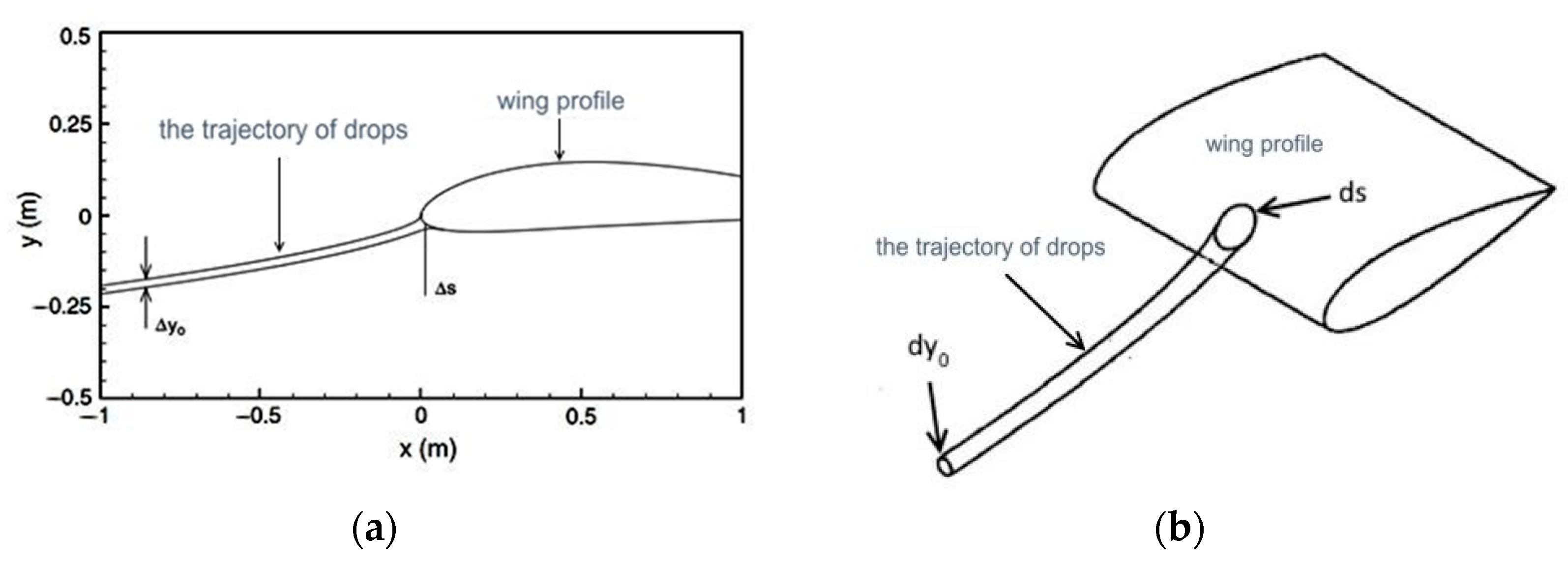
2.2. The Motion of Liquid Droplets as a Continuum in a Gas Dynamic Flow
- All droplets are spherical, with no deformations and breakups of droplets.
- Droplets do not collide with each other, and coalescence/fragmentation of droplets does not take place.
- The effects conditioned by viscous forces are ignored.
- The drag and gravity forces act on droplets.
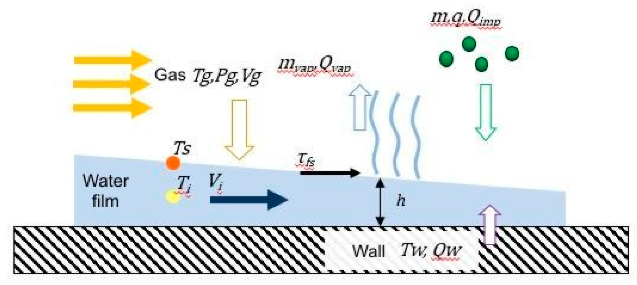
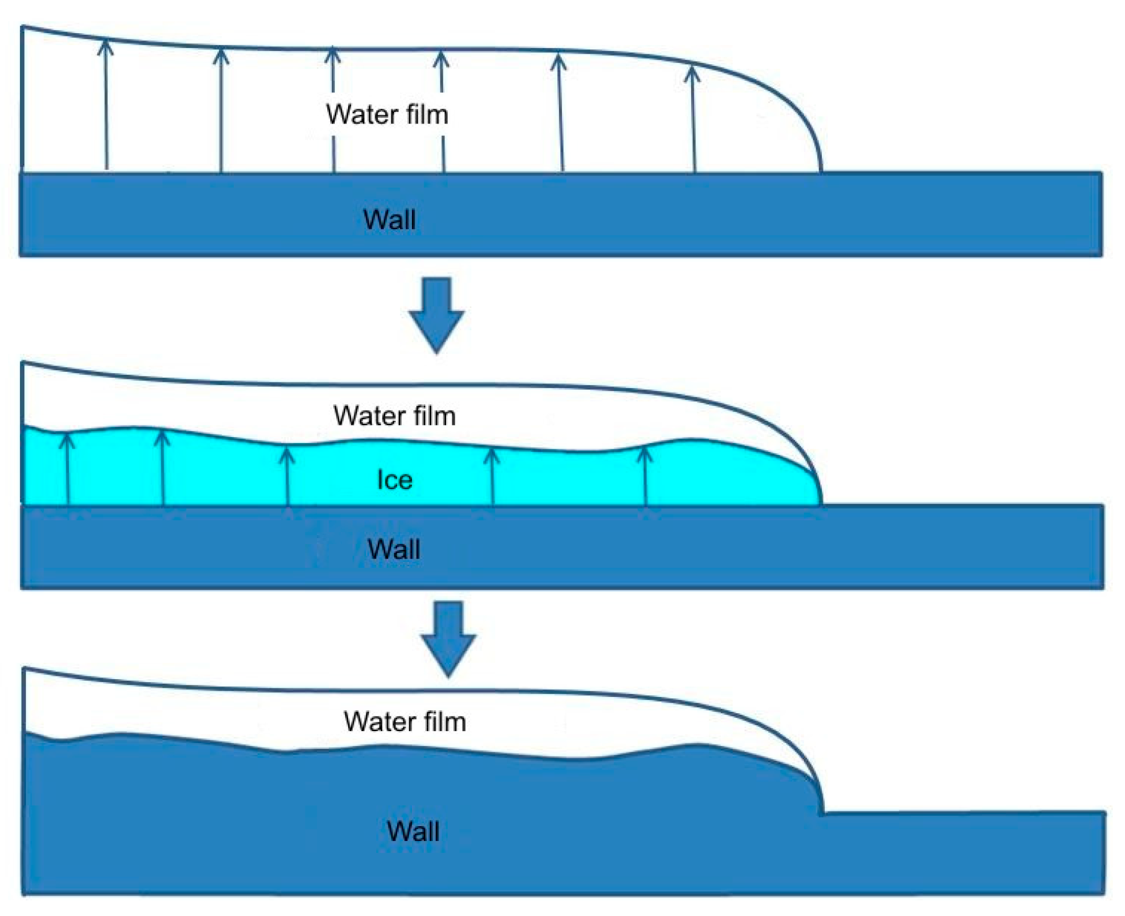
2.3. Calculation of Film Flows on Solid Surfaces
- there is no dissolved air in the liquid film;
- any air–water reaction is not taken into account;
- friction forces are the main driving factors for a liquid film;
- all properties are permanent inside the control volume of interest.
- -
- ice is a heat insulator (), and heat is not transferred between the wall and liquid film;
- -
- there is no heat transfer between neighboring control volumes, and the energy exchange between them is due to the convective heat transfer only;
- -
- a radiative heat flux is considered negligibly small, and its effect is significant, if only the simulation of anti-icing systems is performed ().
2.4. Geometry of the Motion of the Model Surface Faces
3. Results
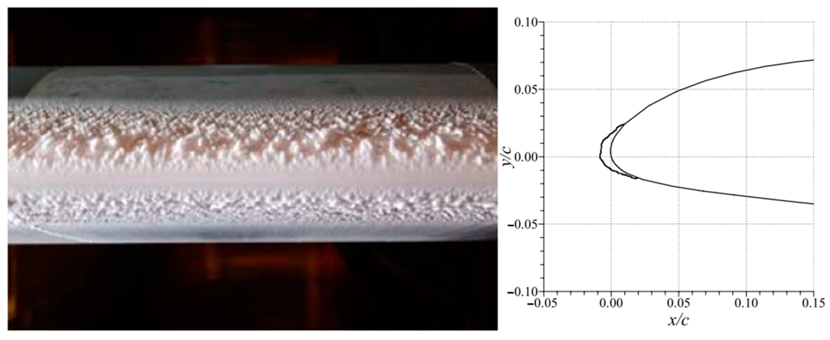
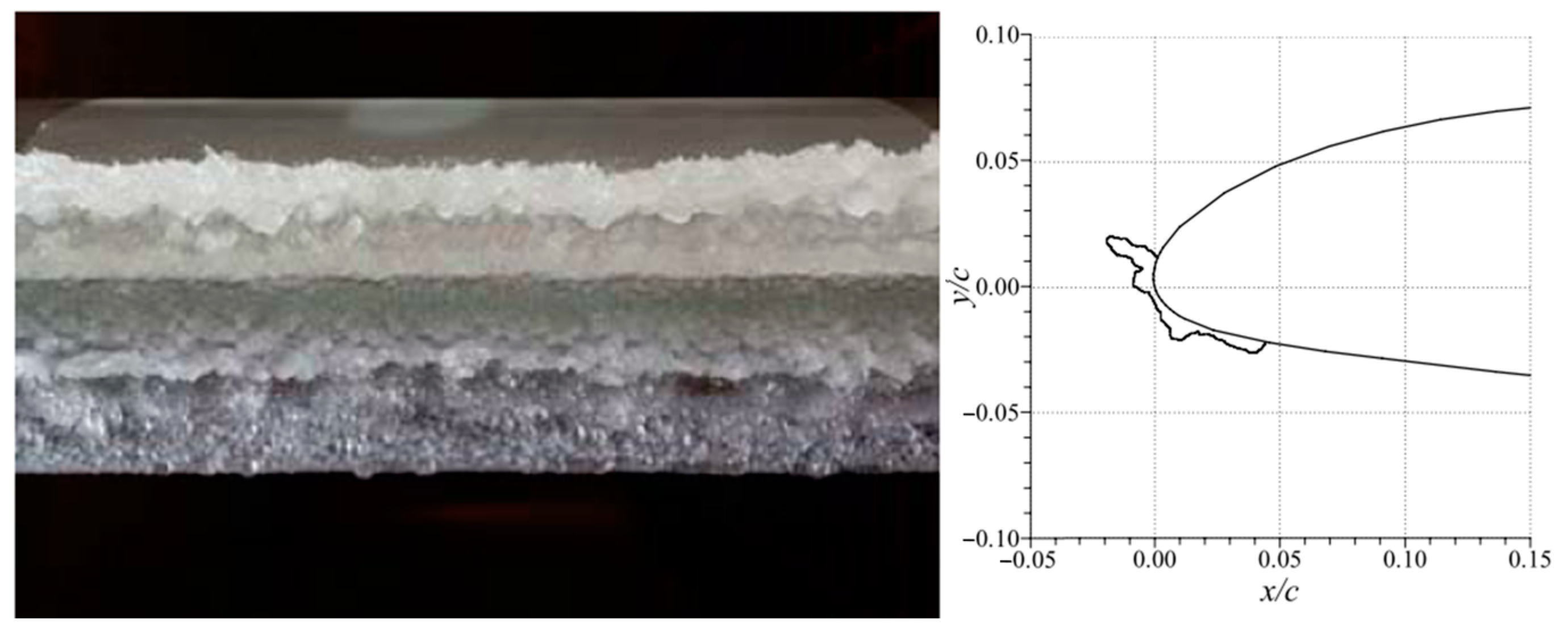
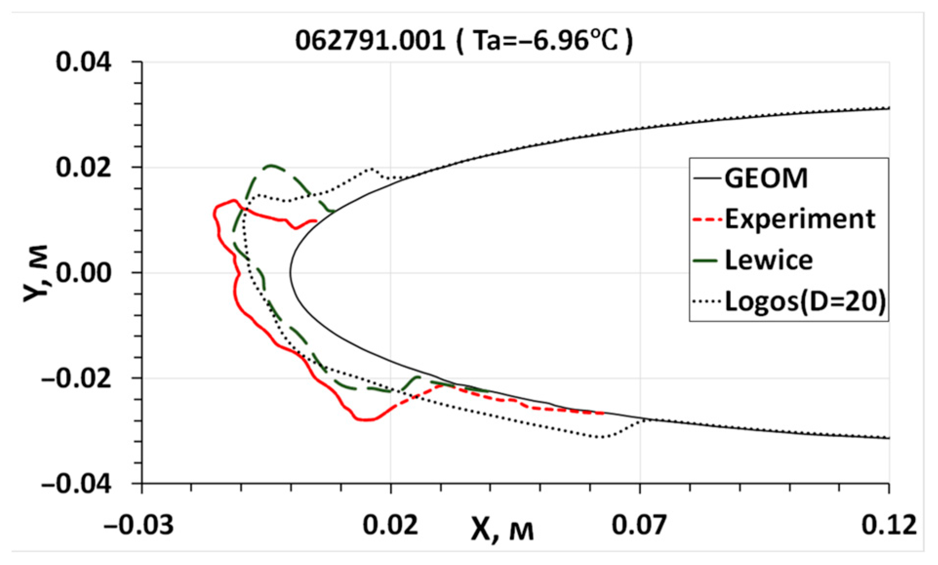
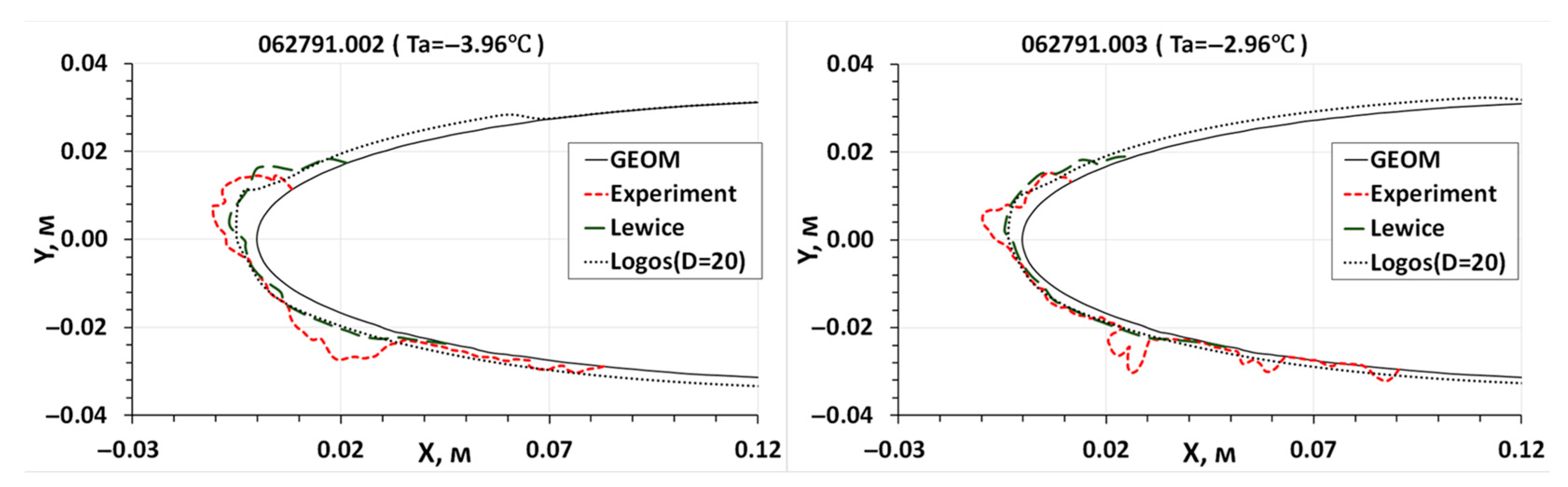
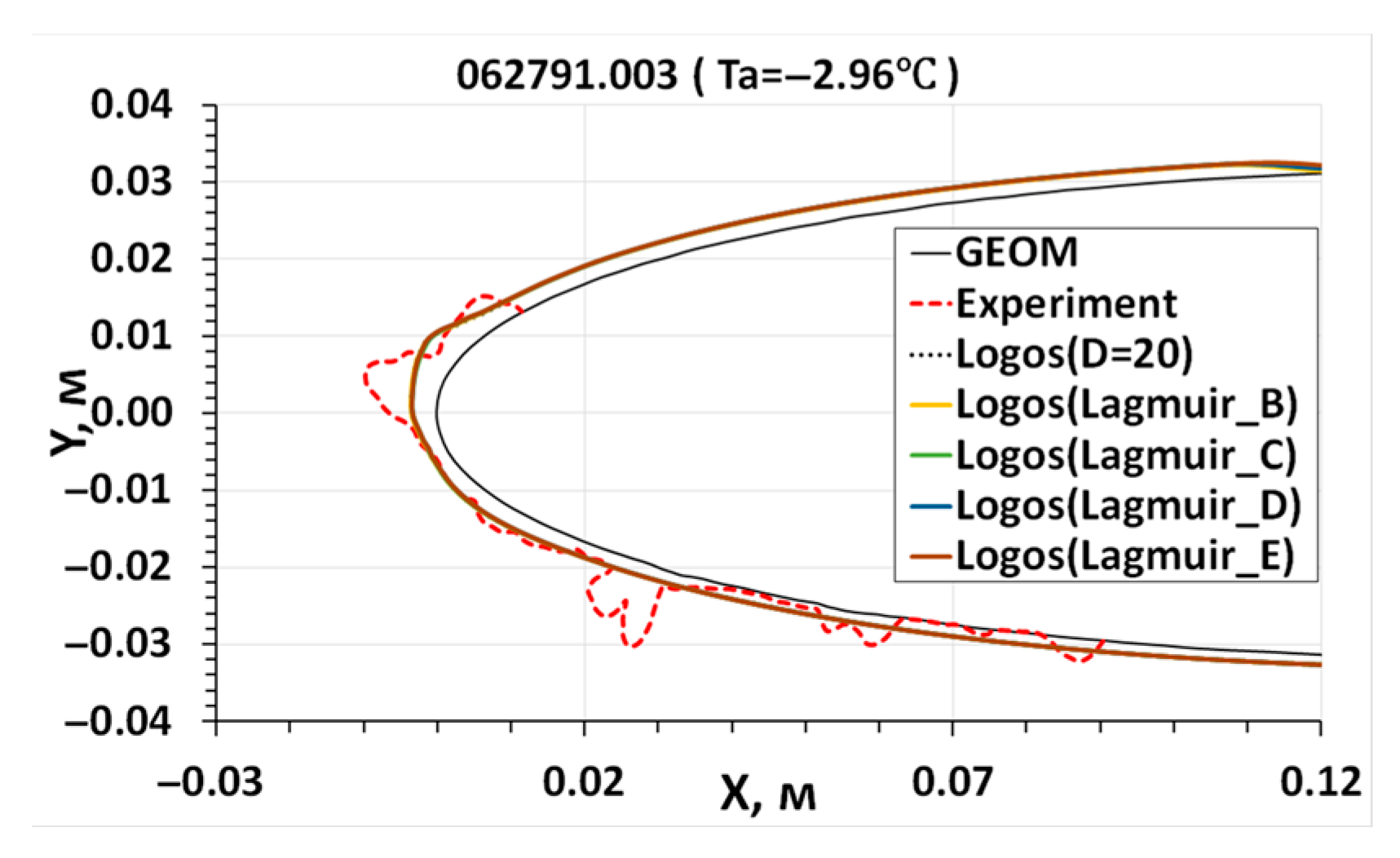
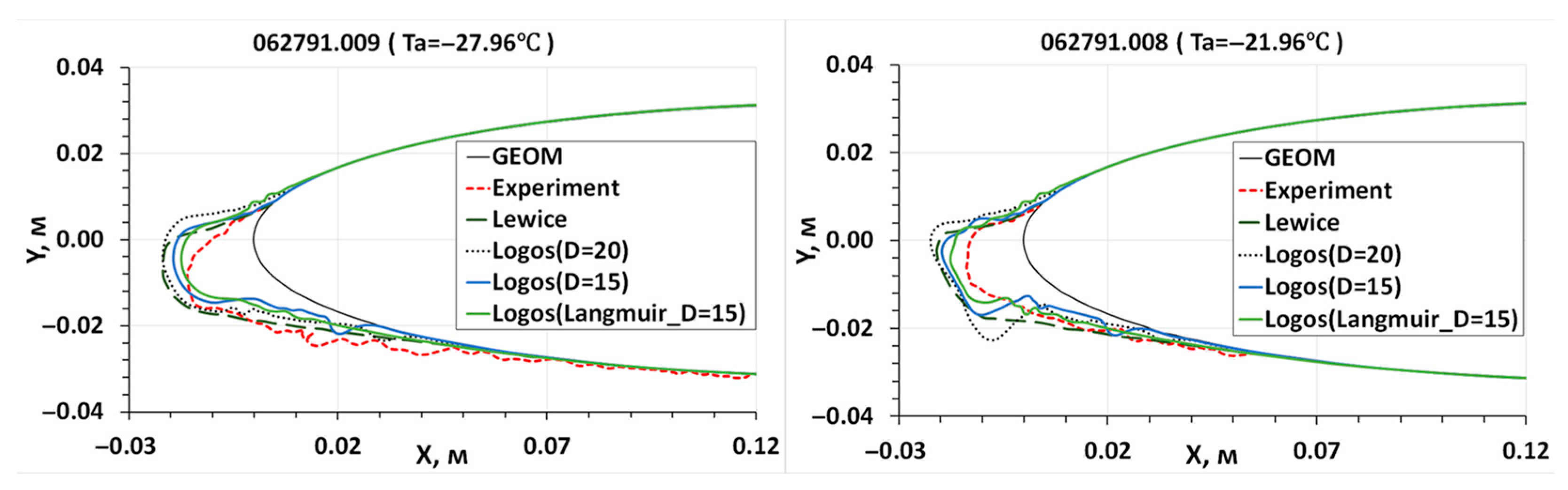
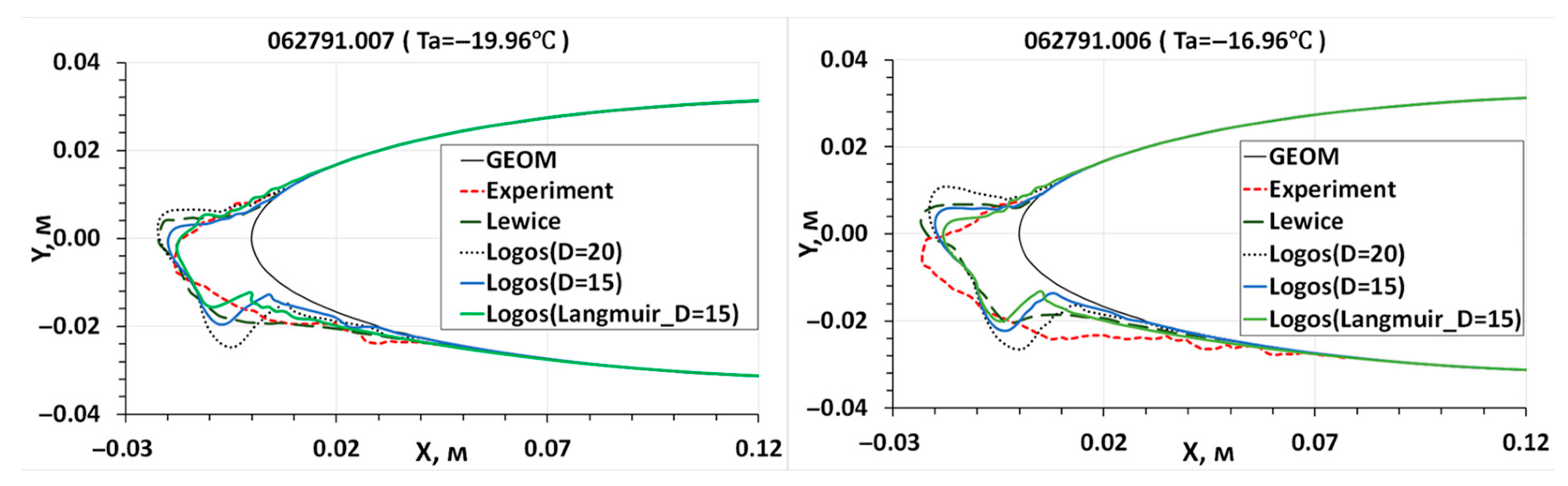
3.1. Ice Accretion Model Validation
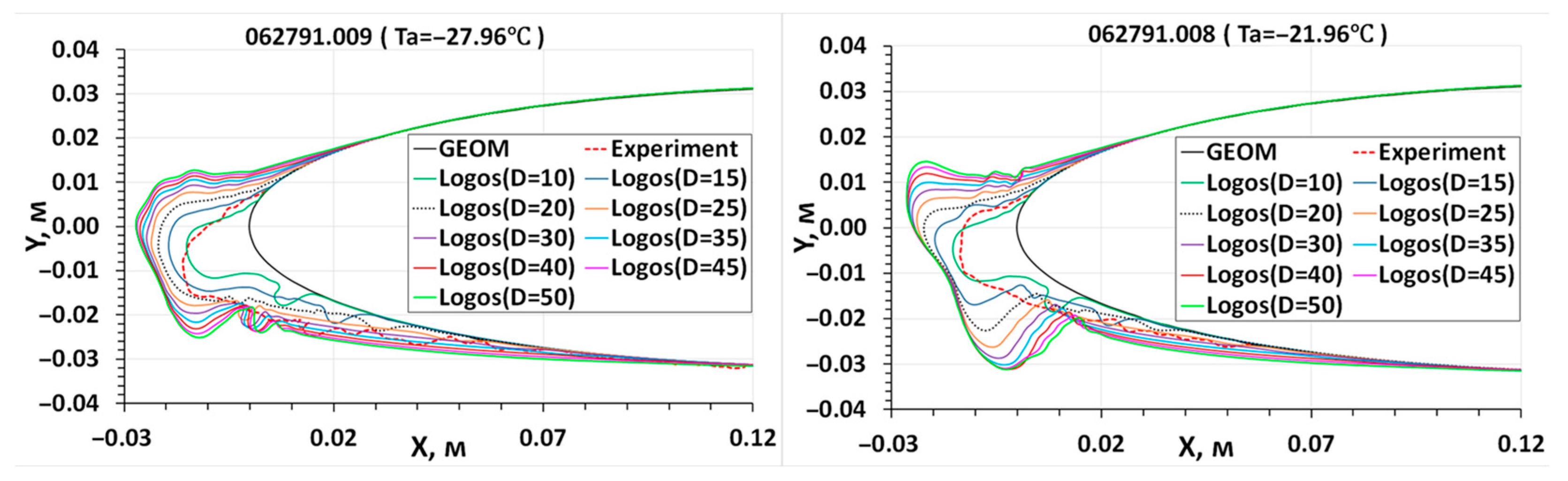
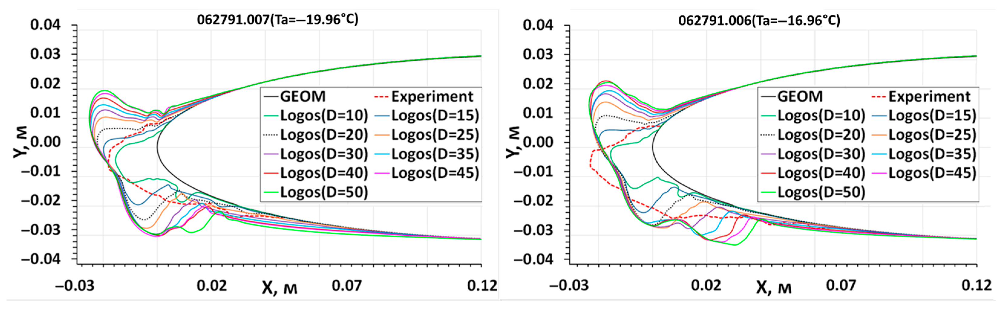
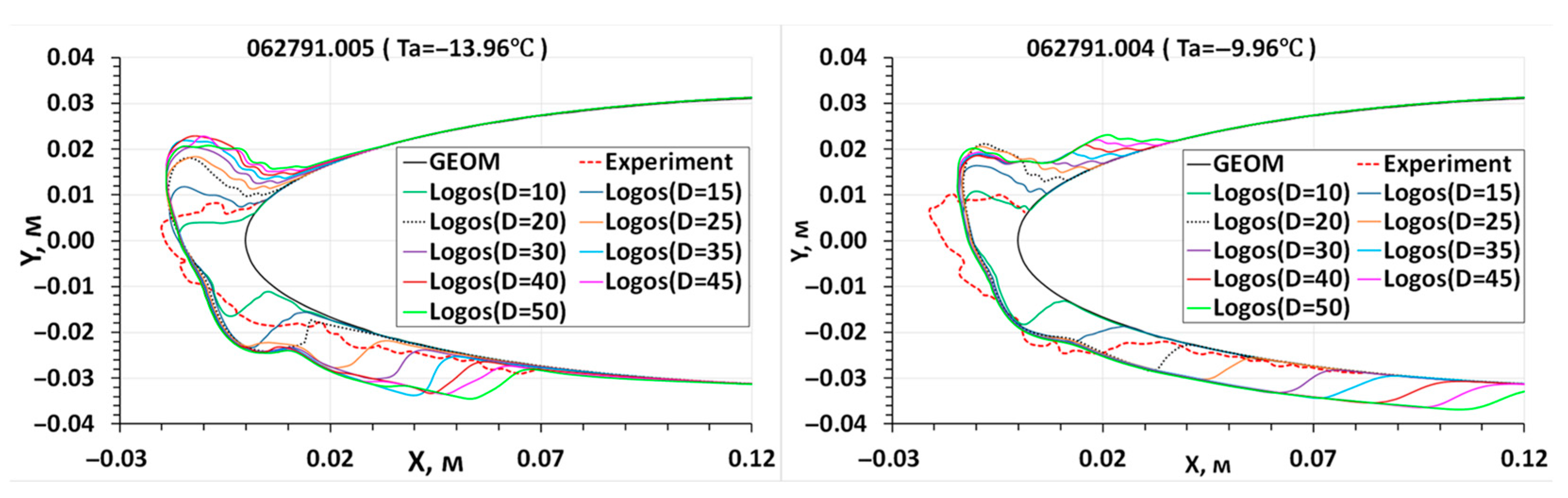
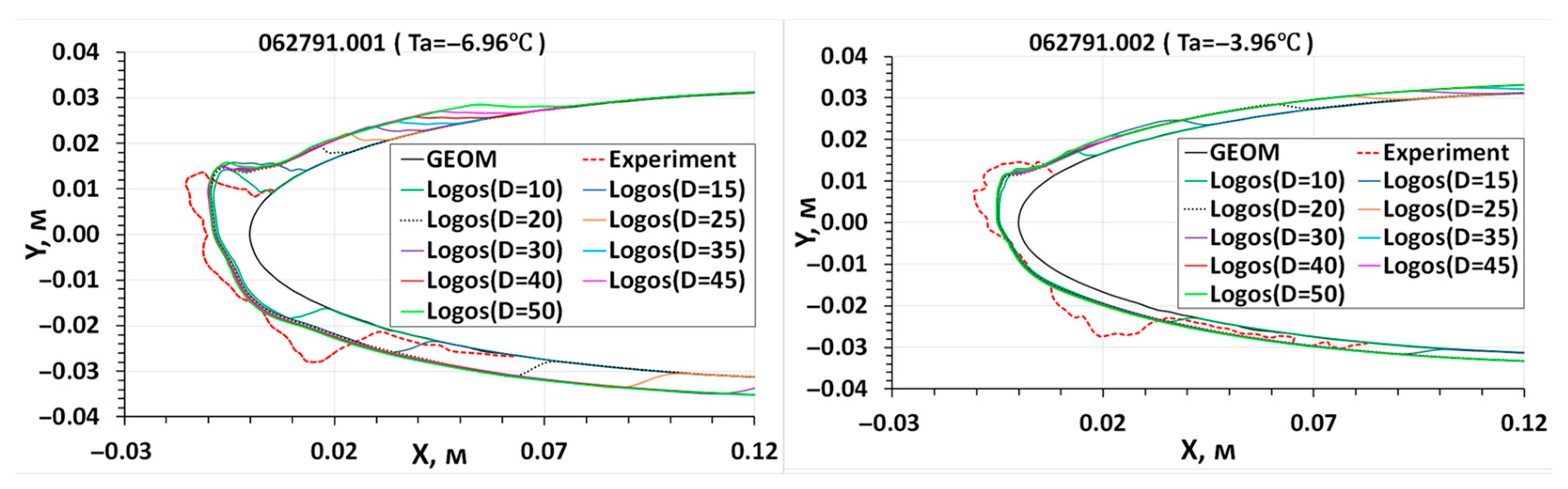
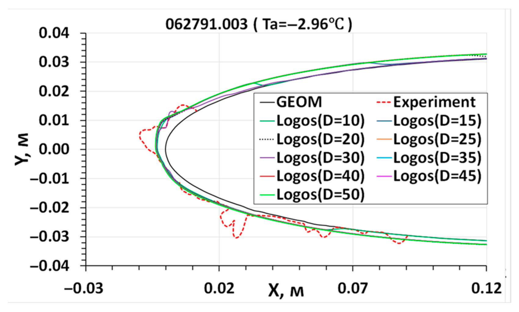
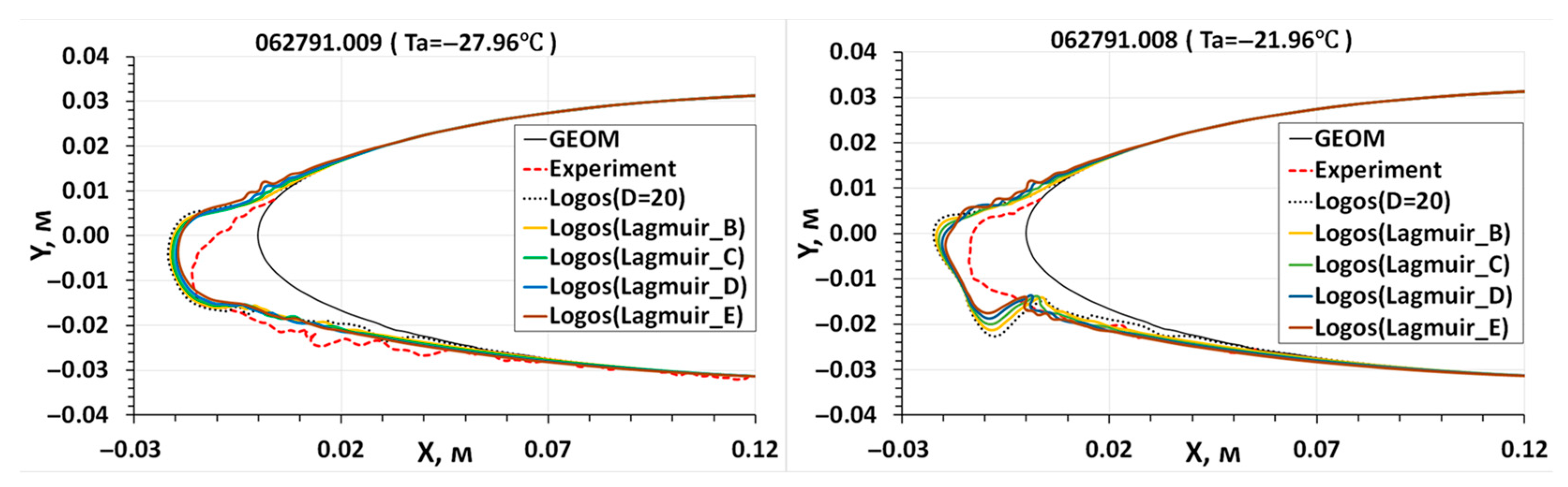
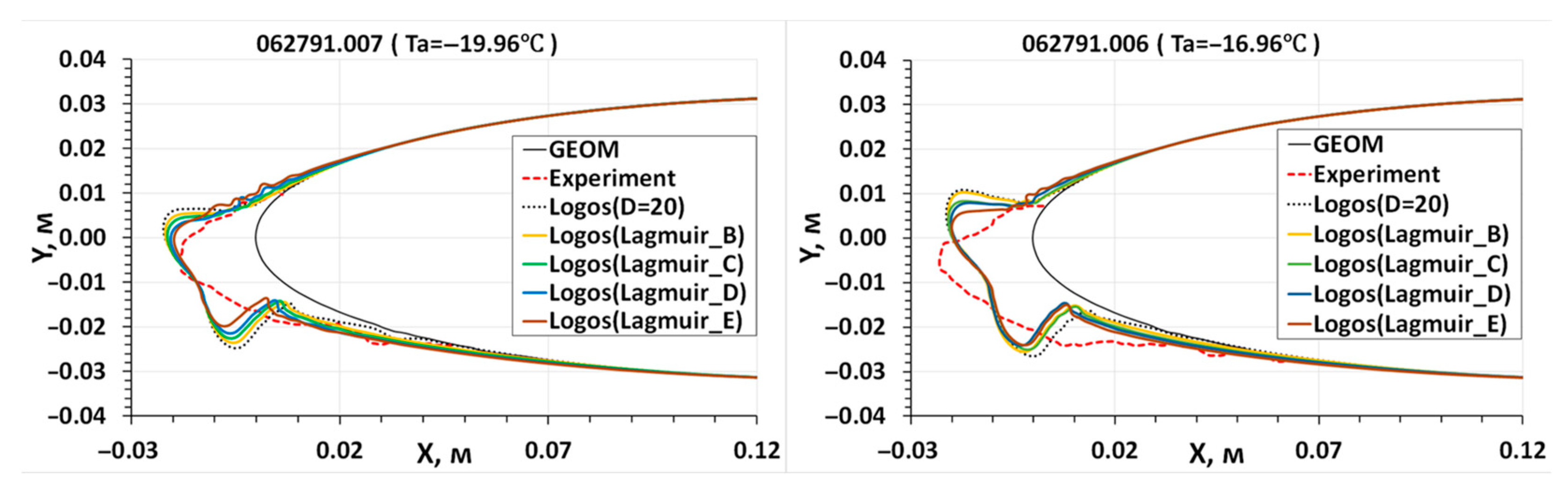
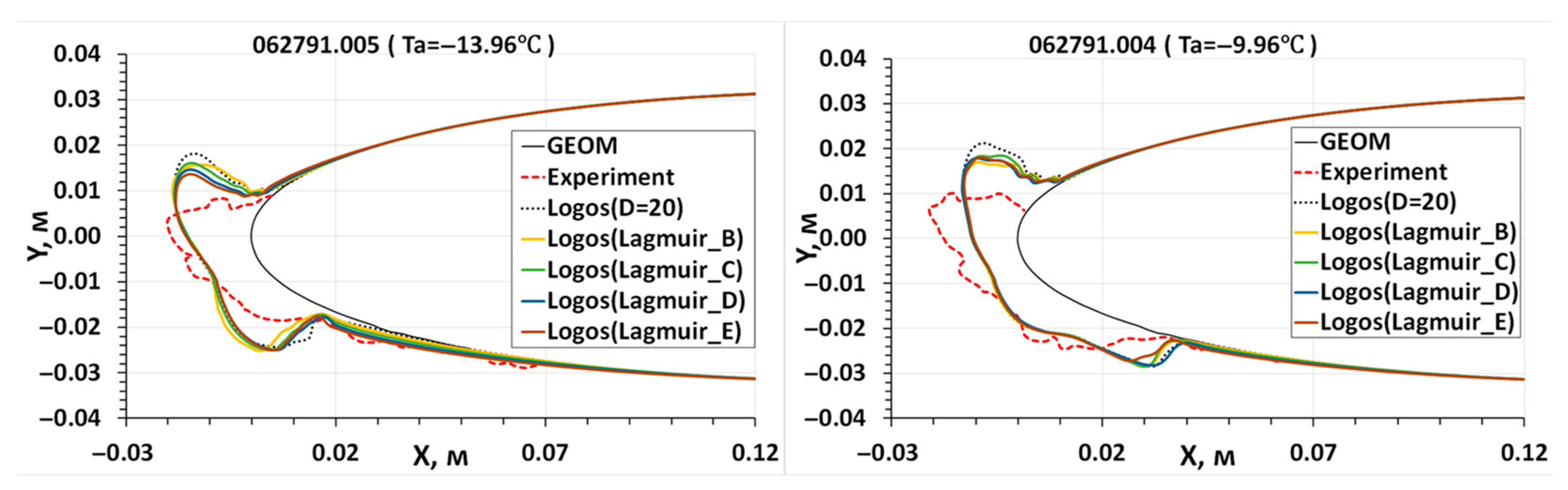
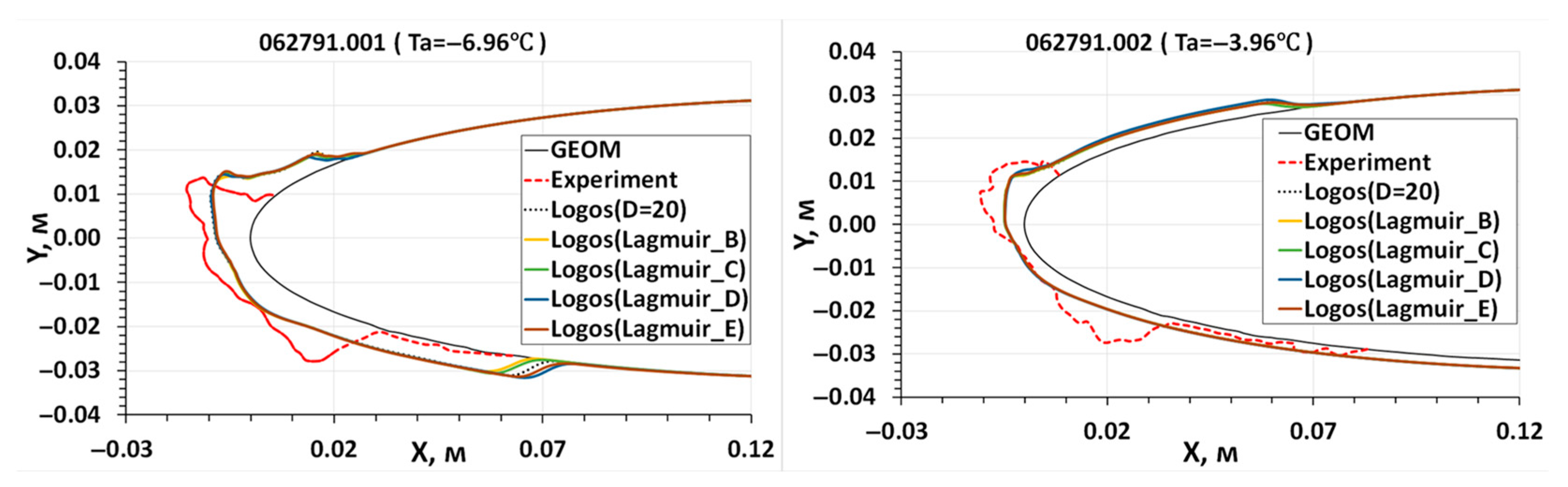
3.2. Studying the Droplet Diameter Effect on Icing
4. Conclusions
- turbulence and roughness of the iced surface of a 3D airfoil on its aerodynamic characteristics;
- the spread water film separation from the surface under the influence of the incoming flow;
- splashing of water droplets impinging on a solid surface and later frozen on the surface.
Author Contributions
Funding
Data Availability Statement
Conflicts of Interest
References
- Kozelkov, A.S.; Pogosyan, M.A.; Strelets, D.Y.; Tarasova, N.V. Application of mathematical modeling to solve the emergency water landing task in the interests of passenger aircraft certification. Aerosp. Syst. 2021, 4, 75–89. [Google Scholar] [CrossRef]
- Kind, R.J.; Potapczuk, M.G.; Feo, A.; Golia, C.; Shah, A.D. Experimental and computational simulation of in-flight icing phenomena. Prog. Aerosp. Sci. 1998, 34, 257–345. [Google Scholar] [CrossRef]
- Lynch, F.T.; Khodadoust, A. Effects of ice accretions on aircraft aerodynamics. Prog. Aerosp. Sci. 2001, 37, 669–767. [Google Scholar] [CrossRef]
- Cao, Y.H.; Tan, W.Y.; Wu, Z.L. Aircraft icing: An ongoing threat to aviation safety. Aerosp. Sci. Technol. 2018, 75, 353–385. [Google Scholar] [CrossRef]
- Myers, T.G.; Charpin, J.P.F. A mathematical model for atmospheric ice accretion and water flow on a cold surface. Int. J. Heat Mass Transf. 2004, 47, 5483–5500. [Google Scholar] [CrossRef]
- Kong, W.; Liu, H. A theory on the icing evolution of supercooled water near solid substrate. Int. J. Heat Mass Transf. 2015, 91, 1217–1236. [Google Scholar] [CrossRef]
- Cao, Y.; Huang, J.; Yin, J. Numerical simulation of three dimensional ice accreation on an aircraft wing. Int. J. Heat Mass Transf. 2016, 92, 34–54. [Google Scholar] [CrossRef]
- Ruff, G.A.; Berkowitz, B.M. Users Manual for the Improved NASA Lewis Ice Accretion Code LEWICE 1.6; NASA-CR-198355 1990.
- Bourgault, Y.; Beaugendre, H.; Habashi, W.G. Development of a Shallow-Water Icing Model in FENSAP-ICE. J. Aircr. 2000, 37, 640–646. [Google Scholar] [CrossRef]
- Hedde, T.; Guffond, D. ONERA Three-Dimensional Icing Model. AIAA J. 1995, 33, 1038–1045. [Google Scholar] [CrossRef]
- RIuliano, T.E.; Brandi, V.; Mingione, G.; de Nicola, C. Water impingement prediction on multi-element airfoils by means of Eulerian and Lagrangian approach with viscous and inviscid air flow. In Proceedings of the 44th AIAA Aerospace Sciences Meeting and Exhibit, Reno, NV, USA, 9–12 January 2006; p. 1270. [Google Scholar]
- Gent, R.W. TRAJICE2—A Combined Water Droplet Trajectory and Ice Accretion Prediction Program for Aerofoils. RAE TR 90054. 1990. Available online: https://ntrs.nasa.gov/api/citations/19970023937/downloads/19970023937.pdf (accessed on 24 March 2023).
- Han, Y. Theoretical and Experimental Study of Scaling Methods for Rotor Blade Ice Accretion Testing. Doctoral Dissertation, The Pennsylvania State University, State College, PA, USA, August 2011. [Google Scholar] [CrossRef]
- Federal Aviation Regulations. Part 25 Airworthness Standards: Transport Category Airplanes, 3rd ed.; with amendments 1–7. JSC «AVIAIZDAT»; 2014. Available online: https://www.ecfr.gov/current/title-14/chapter-I/subchapter-C/part-25 (accessed on 24 March 2023).
- FAA. Federal Aviation Regulation, Part 29 (FAR 29), «Airworthiness Standarts:Transport Category Rotorcraft», Appendix C, (Code of Federal Regulations, Title 14, Chapter 1, Part 29, Appendix C), Superintendent of Documents; Government Printing Office: Washington, DC, USA, 1994; p. 20402.
- Honsek, R.; Habashi, W.G. FENSAP-ICE: Eulerian Modeling of Droplet Impingement in the SLD Regime of Aircraft Icing. In Proceedings of the 44th AIAA Aerospace Sciences Meeting and Exhibit, Reno, NV, USA, 9–12 January 2006. [Google Scholar]
- Honsek, R.; Habashi, W.G.; Aub’e, M.S. Eulerian Modeling of In-Flight Icing Due to Supercooled Large Droplets. J. Aircr. 2008, 45, 1290–1296. [Google Scholar] [CrossRef]
- Rocco, E.T.; Han, Y.; Palacios, J. Super-cooled Large Droplet Ice Accretion Reproduction and Scaling Law Validation. In Proceedings of the 8th AIAA Atmospheric and Space Environments Conference, AIAA Aviation, Washington, DC, USA, 13–17 June 2016. [Google Scholar]
- Wright, W.; Potapczuk, M. Semi-Empirical Modelling of SLD Physics. In Proceedings of the 42nd AIAA Aerospace Sciences Meeting and Exhibit, Reno, NV, USA, 20 January 2004. [Google Scholar]
- Bilodeau, D.; Habashi, W.G.; Fossati, M. Numerical Modeling of Supercooled Large Droplets Re-impingement. In Proceedings of the 21st Annual Conference of the CFD Society of Canada, Sherbrooke, QC, Canada, 6 May 2013. [Google Scholar]
- Jung, S.K.; Kim, J.H. Numerical Model for Eulerian Droplet Impingement in Supercooled Large Droplet Conditions. In Proceedings of the 51st AIAA Aerospace Sciences Meeting including the New Horizons Forum and Aerospace Exposition, Grapevine, TX, USA, 7–10 January 2013. AIAA-2013-0244. [Google Scholar]
- Bragg, M.B.; Broeren, A.P.; Addy, H.E.; Potapczuk, M.G.; Guffond, D.; Montreuil, E. Airfoil Ice-Accretion Aerodynamics Simulation, AIAA–2007–0085. In Proceedings of the 45th Aerospace Sciences Meeting and Exhibit sponsored by the American Institute of Aeronautics and Astronautics, Reno, NV, USA, 1–8 January 2007. [Google Scholar]
- Alekseyenko, S.V.; Prykhodko, A.A. Numerical simulation of icing on a cylinder and an airfoil: Model review and computational results. TsAGI Sci. J. 2013, XLIV, 25–57. [Google Scholar] [CrossRef]
- Amelyushkin, I.A. Study of Two-Phase Flows in Application to Icing Problems and Aerophysical Experiment. Ph.D. Thesis, Central Aerohydrodynamic Institute (TsAGI), Moscow, Russia, 2014. [Google Scholar]
- Galanov, N.G.; Sarazov, A.V.; Zhuchkov, R.N.; Kozelkov, A.S. Application of various ice accretion simulation approaches in the LOGOS software package. In Proceedings of the Journal of Physics: Conference Series, Volume 2099, International Conference «Marchuk Scientific Readings 2021» (MSR-2021), Novosibirsk, Russia, 4–8 October 2021; p. 012029. [Google Scholar] [CrossRef]
- Fletcher, C. Computational Techniques for Fluid Dynamics; Springer: Berlin/Heidelberg, Germany, 1988; Volume 2. [Google Scholar]
- Landau, L.D.; Lifshits, E.M. Theoretical physics. In Hydrodynamics; Nauka: Moscow, Russia, 1988; Volume VI. [Google Scholar]
- Loitsyanskii, L.G. Mechanics of Liquids and Gases; Nauka: Moscow, Russia, 1979. [Google Scholar]
- Kovenya, V.M.; Babintsev, P.V. Application of splitting algorithms in the method of finite volumes for numerical solution of the Navier–Stokes equations. J. Appl. Industr. Math. 2018, 12, 479–491. [Google Scholar] [CrossRef]
- Kovenya, V.M. Splitting algorithms for numerical solution of Navier–Stokes equations in fluid dynamics problems. Prikl. Mekh. Tekh. Fiz. 2021, 62, 48–59. [Google Scholar]
- Kim, J.W.; Dennis, P.G.; Sankar, L.N.; Kreeger, R.E. Ice Accretion Modeling using an Eulerian Approach for Droplet Impingement. In Proceedings of the 51st AIAA Aerospace Sciences Meeting including the New Horizons Forum and Aerospace Exposition, Grapevine, TX, USA, 7–10 January 2013. [Google Scholar]
- Norde, E. Eulerian Method for Ice Crystal Icing in Turbofan Engines. Ph.D. Thesis, University of Twente, Enschede, The Netherlands, 2017. [Google Scholar] [CrossRef]
- Luke, E.; Collins, E.; Blades, E. A fast mesh deformation method using explicit interpolation. J. Comp. Phys. 2012, 231, 586–601. [Google Scholar] [CrossRef]
- Kozelkov, A.S.; Struchkov, A.V.; Strelets, D.Y. Two Methods to Improve the Efficiency of Supersonic Flow Simulation on Unstructured Grids. Fluids 2022, 7, 136. [Google Scholar] [CrossRef]
- Struchkov, A.V.; Kozelkov, A.S.; Zhuchkov, R.N.; Volkov, K.N.; Strelets, D.Y. Implementation of Flux Limiters in Simulation of External Aerodynamic Problems on Unstructured Meshes. Fluids 2023, 8, 31. [Google Scholar] [CrossRef]
- Korotkov, A.; Kozelkov, A. Three-dimensional numerical simulations of fluid dynamics problems on grids with nonconforming interfaces. Sib. Electron. Math. Rep. 2022, 19, 1038–1053. [Google Scholar] [CrossRef]
- Kozelkov, A.; Kurkin, A.; Kurulin, V.; Plygunova, K.; Krutyakova, O. Validation of the LOGOS Software Package Methods for the Numerical Simulation of Cavitational Flows. Fluids 2023, 8, 104. [Google Scholar] [CrossRef]
- Oran, E.; Boris, J. Numerical Simulation of Reactive Flow; Cambridge University Press: Cambridge, UK, 2001. [Google Scholar]
- Schlichting, G. Theory of the Boundary Layer; Nauka: Moscow, Russia, 1974; 712p. [Google Scholar]
- Menter, F.R. Zonal two–equation k–w turbulence models for aerodynamic flows. In Proceedings of the 23rd Fluid Dynamics, Plasmadynamics, and Lasers Conference, Orlando, FL, USA, 6–9 July 1993; p. 2906. [Google Scholar]
- Garbaruk, A.V.; Strelets, M.K.; Travin, A.K.; Shur, M.L. Modern Approaches to Simulation of Turbulence; St. Petersburg Polytechnic University: Saint Petersburg, Russia, 2016. Available online: https://scholar.google.com/citations?view_op=view_citation&hl=ru&user=RegAS60AAAAJ&citation_for_view=RegAS60AAAAJ:dTyEYWd-f8wC (accessed on 24 March 2023).
- Ferziger, J.H.; Peric, M. Computational Methods for Fluid Dynamics, 3rd ed.; Springer: Berlin/Heidelberg, Germany, 2002. [Google Scholar]
- Smirnov, E.M.; Zaitsev, D.K. Finite volume method as applied to hydro- and gas dynamics and heat transfer problems in complex geometry domains. St. Petersburg Polytech. Univ. J. 2004, 2, 70–81. [Google Scholar]
- Soloveychik, Y.G.; Royak, M.E.; Persova, M.G. The Finite Element Method for Scalar and Vector Problems; NSTU: Novosibirsk, Russia, 2007; ISBN 978-5-7782-0749. [Google Scholar]
- Ozgen, S.; Canibek, M. Ice accretion simulation on multi-element airfoils using extended Messinger model. Heat Mass Transfer. 2008, 45, 305–322. [Google Scholar] [CrossRef]
- Hedde, T. Modelisation Tridimensionnelle des Depots de Givre sur les Voilures D’aeronefs. Ph.D. Thesis, Universite Blaise-Pascal, Clermont-Ferrand II, France, 1992. [Google Scholar]
- Messinger, B.L. Equilibrium temperature of an unheated icing surface as a function of airspeed. J. Aeronaut Sci. 1953, 20, 29–42. [Google Scholar] [CrossRef]
- Jiao, X. Face offsetting: A unified approach for explicit moving interfaces. J. Comp. Phys. 2007, 220, 612–625. [Google Scholar] [CrossRef]
- Koshelev, K.B.; Melnikova, V.G.; Strizhak, S.V. Development of iceFoam solver to simulate the icing process. Proc. ISP RAS J. 2020, 32, 217–234. [Google Scholar] [CrossRef] [PubMed]
- Uyttersprot, L. Inverse Distance Weighting Mesh Deformation. A Robust and Efficient Method for Unstructured Meshes. Master’s Thesis, Delft University of Technology Department of Aerodynamics, Brussels, Belgium, 12 February 2014; p. 177. [Google Scholar]
- Ice accretion simulation // AGARD-AR-344.—1997. p. 280.
- Radenac, E. Validation of a 3D ice accretion tool on swept wings of the SUNSET2 program, AIAA Aviation. In Proceedings of the 8th AIAA Atmospheric and Space Environments Conference, Washington, DC, USA, 13–17 June 2016. [Google Scholar]
- Wright, B.W.; Rutkowski, A. Validation Results for LEWICE 2.0, NASA/CR--1999-208690. 1999. Available online: https://ntrs.nasa.gov/api/citations/19990021235/downloads/19990021235.pdf (accessed on 24 March 2023).
- Yugulis, K.; Chase, D.; McCrink, M. Ice Accretion Analysis for the Development of the HeatCoat TM Electrothermal Ice Protection System. In Proceedings of the AIAA AVIATION 2020 Forum, Virtual Event, 15–19 June 2020. [Google Scholar] [CrossRef]
- Shin, J.; Bond, T. Experimental and Computational Ice Shapes and Resulting Drag Increace for a NACA0012 Airfol. In Proceedings of the 5th Symposium on Numerical and Physical Aspects of Aerodynamic Flows Sponsored, California State University, Long Beach, CA, USA, 13-16 January 1992. NASA/TM-105743. [Google Scholar]
- Heinrich, A.; Ross, R.; Zumwalt, G.; Provorse, J.; Padmanabhan, V.; Thompson, J.; Riley, J. Aircraft Icing Handbook; Federal Aviation Administration: Wichita, KS, USA, 1991.
- Langmuir, I.; Blodgett, K. A Mathematical Investigation of Water Droplet Trajectories; Army Air Forces Technical Report 5418; Army Air Forces Headquarters, Air Technical Service Command, University of Illinois at Urbana-Champaign: Champaign, IL, USA, 1946. [Google Scholar]
- Finstad, K.J. Numerical and Experimental Studies of Rime Ice Accretion on Cylinders and Airfoils. Ph.D. Thesis, University of Alberta, Edmonton, AB, Canada, 1986. [Google Scholar] [CrossRef]
- Sokolov, P.; Virk, M.S. Droplet Distribution Spectrum Effects on Dry Ice Growth on Cylinders. Cold Reg. Sci. Technol. 2019, 160, 80–88. [Google Scholar] [CrossRef]


| Case No. | Experiment No. | ||
|---|---|---|---|
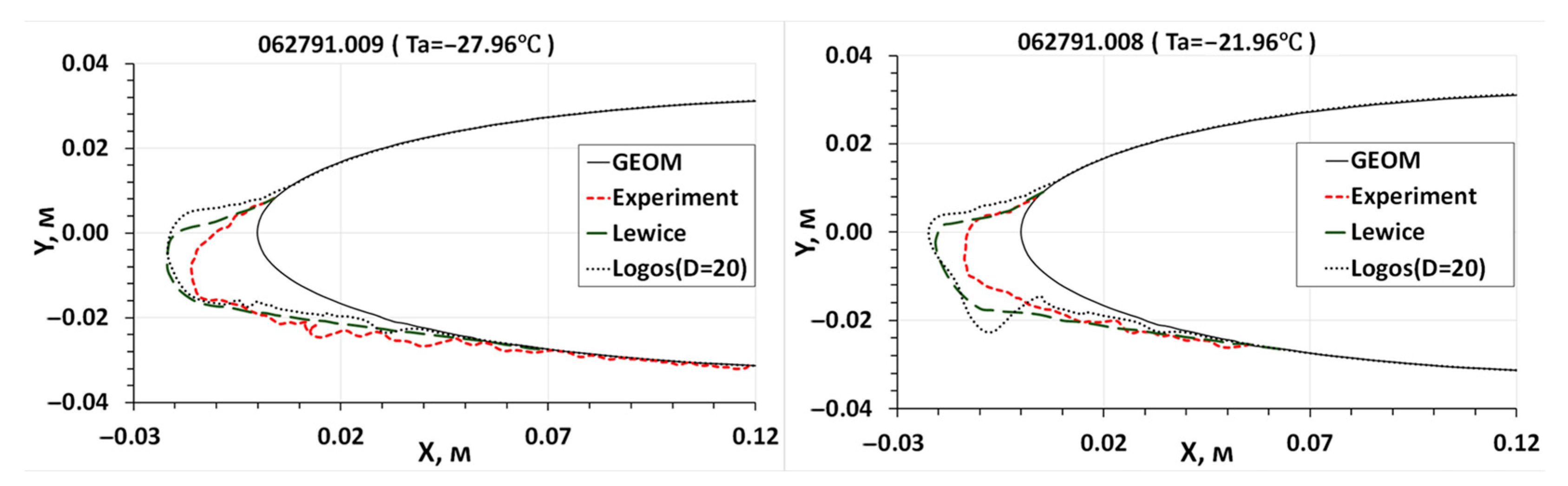
| 1 | 062791.009 | −27.96 | −26.28 |
| 2 | 062791.008 | −21.96 | −20.28 |
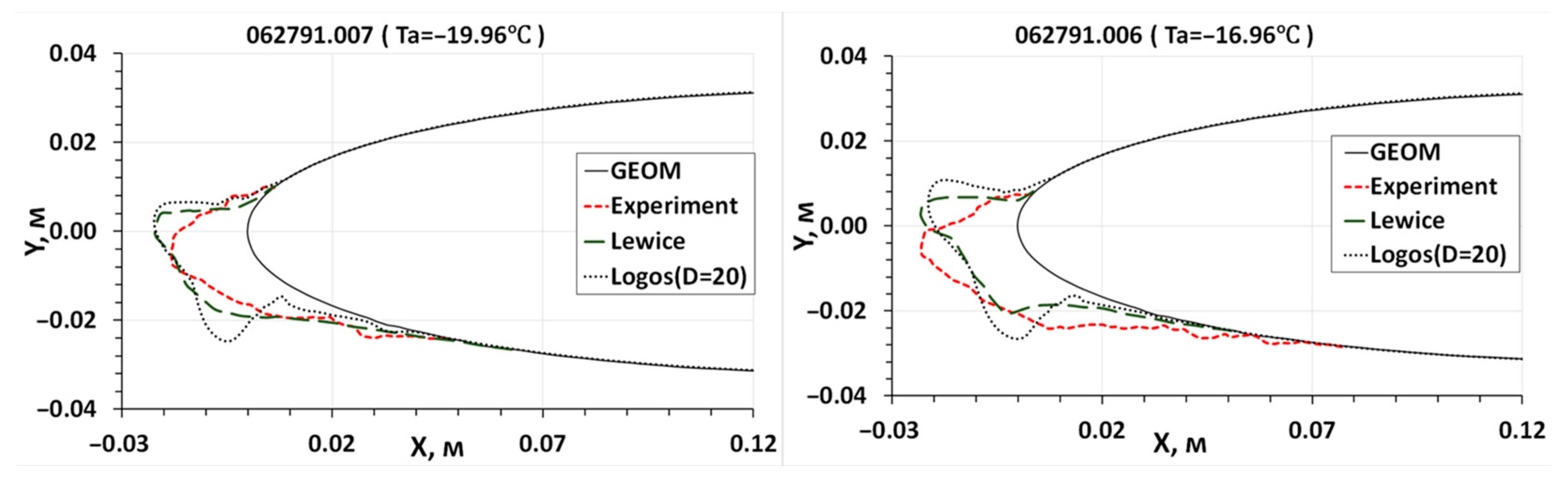
| 3 | 062791.007 | −19.96 | −18.28 |
| 4 | 062791.006 | −16.96 | −15.28 |
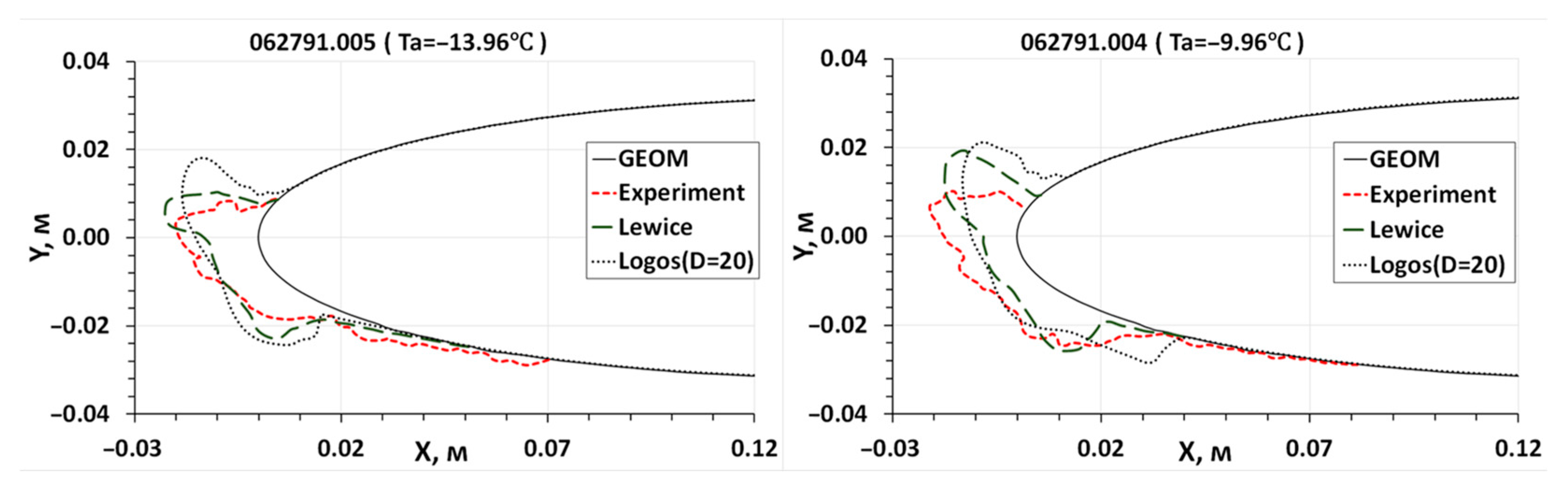
| 5 | 062791.005 | −13.96 | −12.28 |
| 6 | 062791.004 | −9.96 | −8.28 |
| 7 | 062791.001 | −6.96 | −5.28 |
| 8 | 062791.002 | −3.96 | −2.28 |
| 9 | 062791.003 | −2.96 | −1.28 |
| Airfoil Name | Chord, m | V, m/s | P, Pa | α,° | LWC, kg/m3 | MVD, m | Icing Time, min |
|---|---|---|---|---|---|---|---|
| NACA0012 | 0.5334 | 58.1 | 90,760 | 3.5 | 1.3 × 10³ | 20 × 106 | 8 |
| LWC Fraction | A | B | C | D | E | F | G | H | J |
|---|---|---|---|---|---|---|---|---|---|
| 0.05 | 1.00 | 0.56 | 0.42 | 0.31 | 0.23 | 0.18 | 0.13 | 0.10 | 0.06 |
| 0.1 | 1.00 | 0.72 | 0.61 | 0.52 | 0.44 | 0.37 | 0.32 | 0.27 | 0.19 |
| 0.2 | 1.00 | 0.84 | 0.77 | 0.71 | 0.65 | 0.59 | 0.54 | 0.50 | 0.42 |
| 0.3 | 1.00 | 1.00 | 1.00 | 1.00 | 1.00 | 1.00 | 1.00 | 1.00 | 1.00 |
| 0.2 | 1.00 | 1.17 | 1.26 | 1.37 | 1.48 | 1.60 | 1.73 | 1.88 | 2.20 |
| 0.1 | 1.00 | 1.32 | 1.51 | 1.74 | 2.00 | 2.30 | 2.64 | 3.03 | 4.00 |
| 0.05 | 1.00 | 1.49 | 1.81 | 2.22 | 2.71 | 3.31 | 4.04 | 4.93 | 7.34 |
Disclaimer/Publisher’s Note: The statements, opinions and data contained in all publications are solely those of the individual author(s) and contributor(s) and not of MDPI and/or the editor(s). MDPI and/or the editor(s) disclaim responsibility for any injury to people or property resulting from any ideas, methods, instructions or products referred to in the content. |
© 2023 by the authors. Licensee MDPI, Basel, Switzerland. This article is an open access article distributed under the terms and conditions of the Creative Commons Attribution (CC BY) license (https://creativecommons.org/licenses/by/4.0/).
Share and Cite
Kozelkov, A.; Galanov, N.; Semenov, I.; Zhuchkov, R.; Strelets, D. Computational Investigation of the Water Droplet Effects on Shapes of Ice on Airfoils. Aerospace 2023, 10, 906. https://doi.org/10.3390/aerospace10100906
Kozelkov A, Galanov N, Semenov I, Zhuchkov R, Strelets D. Computational Investigation of the Water Droplet Effects on Shapes of Ice on Airfoils. Aerospace. 2023; 10(10):906. https://doi.org/10.3390/aerospace10100906
Chicago/Turabian StyleKozelkov, Andrey, Nikolay Galanov, Ilya Semenov, Roman Zhuchkov, and Dmitry Strelets. 2023. "Computational Investigation of the Water Droplet Effects on Shapes of Ice on Airfoils" Aerospace 10, no. 10: 906. https://doi.org/10.3390/aerospace10100906
APA StyleKozelkov, A., Galanov, N., Semenov, I., Zhuchkov, R., & Strelets, D. (2023). Computational Investigation of the Water Droplet Effects on Shapes of Ice on Airfoils. Aerospace, 10(10), 906. https://doi.org/10.3390/aerospace10100906