Abstract
This paper provides a new method to nonlinear control theory, which is developed from the eigenvalue assignment method. The main purpose of this method is to locate the pointwise eigenvalues of the linear-like structure built by freezing the nonlinear systems at a given time instant in a desired disk region. Since the control requirements for the transient response characteristics are the major constraints on the selection of the disk centre and radius, two different update algorithms are also developed to reshape the disk region by changing the disk centre and radius at each time step. The effectiveness of the proposed methods is tested in both simulations and experiments. A validated three-DOF laboratory helicopter is used for experiments.
1. Introduction
The Eigenvalue assignment method (EAM) is frequently used in control applications to accomplish control objectives since it allows designers to alter the stability and transient response characteristics in a desired way [1,2,3,4]. Undoubtedly, this ability of the EAM arises from the way they can relocate the closed-loop system eigenvalues to some prescribed positions or regions. To achieve this aim, two EAMs were developed, namely, the exact pole placement (EPP) and regional eigenvalue assignment (rEA).
The EPP method has been developed to precisely locate the eigenvalues of the closed-loop system at the desired locations on the left side of the complex plane and then keep these eigenvalues there throughout the entire process. As is well known, all control methods possess their own disadvantages. The most distinct disadvantage of the EPP method is the excessive control effort required to ensure that the locations of the closed-loop eigenvalues are unchanged. Additionally, this strict constraint on the eigenvalue locations also reduces the design flexibility. Therefore, many researchers have developed different rEAs, aiming specifically to locate the closed-loop eigenvalues in user-defined regions rather than at some fixed locations. This approach provides more flexibility than other methods [5,6].
One of the most important considerations in rEA is the selection of the region shape and location because they have a great effect on the system response and control effort. In the literature, previous studies have developed different bounded or unbounded regions formed as a disc, sector, ellipse, etc., for the linear systems [5,6,7,8]. The disc or circular region is one of the most used bounded regions in rEA [9,10,11,12]. The disc parameters, namely the disc centre and radius, can be determined, considering the control requirements for the stability margin and the maximum overshoot [13]. Since the eigenvalues are only allowed to locate in a circular region on the left half of the complex plane, the system responses can be shaped as required. The desired system response can be produced by either shifting the centre of the disc with a fixed radius or by changing the radius of the disc with a fixed centre. In these studies, a fixed region has been selected.
Another important issue in the rEA is to derive a control law, enabling the closed-loop system eigenvalues to be located within a defined region. The Linear Matrix Inequality (LMI) method is one of the most frequently used methods in rEA. Ling [14] used the LMI method to control a MIMO system. The algorithm was tested in simulations and the results showed that the desired performance was achieved. Another LMI approach was used to design a controller for a power system [15]. A guaranteed-cost reliable controller with a regional pole placement method was designed to tackle with the cases where the actuators were faulty. Besides providing the guaranteed cost, the designed fault-tolerant controller was able to shape the transient response successfully according to the design criteria defined in terms of damping ratio, settling time and stability. Wisniewski et al. proposed a regional pole placement based approach to ensure the minimum damping factors for discrete-time systems by placing the eigenvalues in some non-convex regions. The experimental and simulation results showed that the method had created a reasonable balance between the mathematical approximation accuracy and computational complexity [16]. In another approach, the LMI method was used to allocate the partial eigenvalues of a linear time-invariant system in three different regions, i.e., strip, sector and disc, instead of the entire system’s eigenvalues [17]. Then, a set of simulation studies were performed to examine the effectiveness of the approach, and the results showed that the partial eigenvalue allocation was successfully performed with a reliable accuracy. Although the LMI-based rEA method has been tested both in simulation and experimental studies, these studies have been limited to linear systems, and the fixed regions have been considered.
The rEA using the LMI method is generally used for linear systems. However, some approaches developed for nonlinear systems are also available in the literature. Baker et al. have designed a robust feedback controller by using the rEA solved by LMI approach to deal with Lipschitz-type nonlinearities in continuous-time systems [18]. In this study, three different design procedure were established. In the first case, the only aim was to place the eigenvalues corresponding to the linear parts of the controller and observer to ensure the asymptotic stability. On the other hand, in other cases defined in [18], the eigenvalues corresponding to the linear part of the controller and observer were placed in two separate regions. Moreover, the performance criterion was included to the rEA in the third case to ensure the robustness against the bounded nonlinearities. This study differs from the literature in that it takes nonlinearity into account and defines separate regions rather than a single region. However, the desired region is still defined as fixed and does not change over time. Additionally, although the nonlinearity of the system is taken into account, the rEA method was used to place the eigenvalues of the linear part of the system into two separate regions. The rEA can be not only used for some hypothetical systems but also real systems. In a previous study [19], an alternative rEA approach was developed for the flight control design to offer a solution of the tracking problem of an unmanned aerial vehicle. In this approach, the eigenvalues can be placed in multiple regions instead of a single specific region to improve the tracking performance and provide more design flexibility than the traditional approach. There are also different studies in the literature using rEA with LMI [20,21,22,23,24]. Although the LMI-based rEA method is a very frequently used method, as can be seen from the literature, it has not been used in nonlinear systems and the selected regions are defined as fixed regions.
In the literature, besides the LMI method, there are also different rEAs. In [25], the harmony search algorithm was applied to design a state feedback control for a robust eigenvalue assignment in either a single circular region or a set of non-intersecting circular regions. The results showed the proposed method achieved better robustness against the uncertainties with an upper bound, and a Riccati-equation-method-based approach was unable to place the eigenvalues in the desired region. A PID controller is also used with regional pole assignment in the literature. A new robust discrete-time gain-scheduled PID controller method was proposed in [26]. The method depends on regional pole placement using quadratic cost function, and a parameter-dependent Lyapunov function was used to guarantee closed-loop system stability. The results showed that the desired performance was achieved by locating the eigenvalues of the closed-loop system in the user-defined region. In another approach using rEA with quadratic cost function, a robust PID controller was designed [27]. LMI regions and the extended original derivative of the Lyapunov function were utilised to stabilise the system and design controller for uncertain polytopic systems. The results showed that all eigenvalues of the closed-loop system were located in the user-defined LMI region using the proposed method. Another approach for assigning the closed-loop eigenvalues within a user-defined region is to optimally locate the eigenvalues within the desired region. Furuta and Kim proposed a new theorem using a modified Riccati equation for both continuous and discrete systems [7]. In this theorem, all eigenvalues of the closed-loop linear system can be located in a disc region by a state feedback optimal control law. They also investigated the robustness of the control approach by evaluating the gain and phase margins. In [28], the linear quadratic regulator theory was used, and the optimal controller gain was obtained by solving a matrix Riccati equation. The proposed algorithm differs from other studies in the literature [7,29,30] in that it locates all eigenvalues of the closed-loop system inside a disc with a maximum desired region area in the logarithmic spiral corresponding to a desired damping ratio. As seen from studies in the literature, the rEA method was developed using linear control methods. However, there is a lack of development of nonlinear control rules for rEA in nonlinear systems. Additionally, studies have been carried out on the control rule that will place the eigenvalues in a fixed region.
The state-dependent Riccati equation (SDRE) can be also used to design the rEA controller for nonlinear systems. In [31], a state-dependent regional pole assignment controller design was proposed for a class of nonlinear systems. The SDRE was modified using the given disc parameters to ensure that eigenvalues located into the desired disc using the modified optimal control law. The method was modified from the given study in [7] to derive a state-dependent feedback control law enabling the pointwise eigenvalues of the closed-loop system matrix to be located in a desired disc region at each time step. The effectiveness of the method was tested experimentally using three-DOF helicopter setup, and the results were compared with the linear pole assignment method developed in [7]. This method was combined with the sliding mode control method in another study [32]. The experimental study results revealed that the maximum overshoot and settling time can be decreased if the disc centre is selected to be sufficiently further away form the imaginary axis and the disc radius is sufficiently small. Even though these studies differ in terms of using the nonlinear control rule, they are similar to other studies in the literature in terms of region selection and the fact that the selected region is fixed.
In this study, a suboptimal control law based on an rEA method using the disc geometry is introduced to control a class of nonlinear systems that can be parameterised in a linear-like form, mimicking a linear time-invariant (LTI) system at each instant of time. The main contribution of the proposed method is that it offers a way to select the suitable disc parameters in the rEA method. The selection of the parameters (centre and radius) of the disc is the most important issue in this method [7,28]. As mentioned previously, the selected disc region affects the stability, control efforts and transient response characteristics. When the disc centre is chosen further away from the imaginary axis, higher control efforts are needed. However, it is not true in some cases–for example when high inertial system is intended to behave similarly to highly manoeuvrable systems. On the other hand, a disc whose centre is closer to the imaginary axis and whose radius increases results in longer settling times, more oscillatory response and lower stability margin of the system. Due to this fact, the disc parameters should be selected in accordance with the control and stability requirements. Therefore, this paper introduces two update algorithms to determine the disc parameters online which are not handled in the previous studies. The key contributions of the proposed method can be listed as follows:
- 1.
- We extended the rEA that had been proposed for linear systems in [7] to the state-dependent rEA for controlling the “frozen” nonlinear systems.
- 2.
- In our previous studies [31,32], all pointwise eigenvalues of the “frozen” closed-loop system of the nonlinear systems were located in the desired fixed disc region at each time step by using the state-dependent rEA. In this study, we propose two new algorithms that are used to update the disc parameters depending on the locations of the pointwise eigenvalues at the current time for improving the stability and response characteristics according to the design criteria.
2. Methodology
The rEA using disc geometry was first developed for linear systems to place the closed-loop system eigenvalues of the linear system into a user-defined disc. This approach is also applied to the control of the nonlinear systems. First, the nonlinear system is restructured in a linear-like form consisting of the state-dependent system and input matrices by using an extended linearisation method. Then, the system and input matrices of this parameterised system are evaluated at the current time and they are kept constant from the current time instant to the next time instant. This approach enables a different linear system to be created at each time instant. Then, a state-dependent feedback control law is used to enclose the open-loop linear system at each time instant so that the pointwise eigenvalues of the closed-loop system can be placed inside the defined disc. The difference of this approach from the linear approach is that in the linear case, the locations of the eigenvalues in the disc are fixed, whereas in the nonlinear case, the locations of the pointwise eigenvalues can move inside the disc at each time instant because of the changing dynamics of the system. In this section, we will first describe the methodology of the state-dependent regional eigenvalue assignment (SDREA) introduced in our previous studies [31,32]. Then, we will define two different update algorithms to update the disc parameters at each time instant, and we will complete the section with a simulation study to verify the effectiveness of the proposed algorithms.
2.1. State-Dependent Regional Eigenvalue Assignment for Control of Nonlinear Systems
Consider the nonlinear system defined as
where is the state vector and is the control input vector. and with are known nonlinear functions.
To design a state feedback control for the nonlinear system (1), it is firstly parameterised into a linear-like structure using the extended linearisation technique (See [33] for more details). This parameterisation results in
where is a continuous state-dependent matrix-valued function. If the following two conditions are met, (2) can be achieved.
- Given a bounded open set , is a continuously differentiable vector-valued function; that is, .
- Given a bounded open set , the origin is an equilibrium point of the system (1) with ; that is, .
The following proposition guarantees the existence of the parameterisation of .
Proposition 1
(See [33]). Let be such that and . Then for all , a state-dependent coefficient (SDC) parameterisation (2) of always exists for some .
Then, the nonlinear system (1) can be rewritten in the SDC matrix form as
where and are SDC matrices. For a given vector, x, and have constant values and the linear-like SDC structure (3) can be regarded as an LTI system at each time step. Therefore, a state-feedback control law is derived using a state-dependent feedback control law given by
where is the state-dependent feedback gain matrix. In this study, the gain matrix K is determined by using the rEA method so as to ensure that the pointwise eigenvalues of the closed-loop systems can be kept in the desired disc region at each time step. For the nonlinear case, and in (3) are computed at each time instant to produce a linear-like system comprising of and (see [33] for more details) and (3) is rewritten as
In the rEA procedure, the region to which the eigenvalues are assigned must be defined. Figure 1 illustrates a bounded disc D that is a closed circular region with its centre at located on the negative real axis and a radius of r.
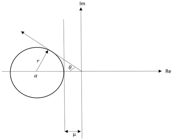
Figure 1.
Disc D in the left of the complex plane.
The disc parameters ( and r) are obtained from the desired stability margin () and the damping ratio (). Therefore, these parameters affect the time response characteristics of the system such as maximum overshoot and settling time. To obtain and r, the following geometrical relationships are introduced
From Equations (6)–(8), the limits on the disc parameters can be found according to the constraints on the maximum overshoot and damping ratio. After the disc parameters are determined, a suitable control law that does not violate the limit of the disc, thereby causing the pointwise eigenvalues of the closed-loop system to be located inside the boundary of the disc, should be obtained. This need can be satisfied by using the state-dependent regional eigenvalue assignment method (SDREAM) for nonlinear systems, which has been previously extended from the study [7] developed for the linear systems. Now, it will be reviewed for the sake of completeness as follows:
Lemma 1.
Consider the matrix equation defined as
where * denotes the conjugate transpose, is a semi-positive definite matrix and are the eigenvalues of at each time instant . If a positive definite matrix exists for every , remain inside the specified disc with its centre at α and a radius of r for every .
Proof.
and are defined as the eigenvalue and the eigenvector of , respectively. Then,
If the both sides of (9) are multiplied by and , the following equation is derived
Defining the pointwise eigenvalues as at each time instant and substituting it into (12), then (12) becomes
and (13) can be rewritten as
where and . Therefore, the following inequality is obtained
As can be seen from (15), the inequality defines a disc. Therefore, stay inside the disc D at each time instant . Accordingly, also stay inside the disc D for the whole time range. □
Using Lemma 1 and Assumption 1, the following theorem gives the condition to guarantee that the eigenvalues of the closed-loop system matrix can be located in a desired disc defined by (15) at each time instant .
Assumption 1.
The pairs and are pointwise stabilisable (or controllable) and detectable (or observable) for all x.
Theorem 1.
Consider the following matrix equation
If and , all eigenvalues of the closed-loop matrix are located in a desired disc at each time instant .
The following theorem is presented to obtain the state-feedback control law at each time instant
Theorem 2.
The feedback control law at time instant
and
locates all eigenvalues of inside a desired disc that is centred at α with a radius of r. Here, , obtained at , is a positive definite symmetric solution of the Riccati equation given as
where the weighting matrix is selected arbitrarily, and is a matrix such that the pair () is observable.
Proof.
Using Lemma 1 and Theorem 1 together with , it is proven that all eigenvalues of locate in the desired disc D at each time instant . □
Remark 1.
The selection of the weighting matrices R and Q has an effect of the locations of . moves inside the disc D by changing the weighting matrices R and Q.
As can be seen, SDREAM is able to place the pointwise eigenvalues of the closed-loop system in the defined fixed disc at each time step, and the location of the eigenvalues changes depending on the state variables sequentially. Although better results are obtained from SDREAM than the rEA method developed for linear systems in the nonlinear control application, it still suffers from some disadvantages due to the use of the fixed disc region. For example, if a disc with a very small radius or the disc centre is chosen too far from the imaginary axis, excessive control inputs are required, causing some practical issues in real-time applications due to physical limits of real systems or their actuators. Therefore, the system responses shaped by the constraints on the settling times and maximum overshoots must remain within a certain limit. As will be seen in the following sections, the two different algorithms are developed to improve the system responses. Both algorithms are based on the idea that the disc parameters can be updated at each time instant according to the positions of the eigenvalues at the previous time instant.
2.2. Update Algorithm 1
In this algorithm, the radius of the disc is reduced at each time step, considering the locations of the “frozen” closed-loop system’s eigenvalues at the previous time instant, while keeping the centre of the disc constant. In this way, the stability margin and damping ratio increase at each time instant without exceeding the system limits.
The initial condition value of and r, i.e., and , are obtained from the stability margin and damping ratio using Equations (6)–(8). The first control input is calculated from these values and applied to the system. Then, the eigenvalue locations of the closed-loop system are determined. The eigenvalue farthest from the centre is selected and the distance of this eigenvalue from the centre of the disc is computed. In the next time step, the new radius of the disc is taken as the distance from the farthest eigenvalue to the centre, and the control input is recalculated at the next time instant; finally, the above steps are repeated. This process continues until the system reaches equilibrium.
The proposed Update Algorithm 1 is explained in details from the mathematical point of view as follows:
Algorithm 1
(Update Algorithm 1).
Step 1. The disc centre is fixed at each time step and calculated only once from the initial stability margin and damping ratio using Equations (6) and (7). The initial condition value of is obtained from the initial stability margin and damping ratio using Equation (8). However, the radius of the disc that will be used in the next time step is the distance of the eigenvalue farthest from the centre at the current time instant .
Step 2. The locations of the eigenvalues and their distance from the centre at the time instant are determined by the following equations
where denotes the ith eigenvalue. and are the projections of on the real and imaginary axes of the complex plane at the time instant .
Step 3. The distances of the eigenvalues from the centre of the disc at the time instant are determined using the following equation
Step 4. The new disc radius is chosen. The new disc radius at the next time instant is the positive maximum value of the calculated at the time instant which is mathematically expressed by
Step 5. Now, considering the updated radius of the disc, the control law is recomputed at each time instant by using Equation (27).
Theorem 3.
Given r as and the matrix equation in Theorem 1, consider the following matrix equation
If and , all eigenvalues of the closed-loop matrix are located in a desired disc that is centred at α with a radius of at each time instant . Here, is obtained from Equation (25) with the initial condition of .
The following theorem which is derived from Theorem 2 by replacing r with is here introduced to obtain the state-feedback control law at each time instant .
Theorem 4.
The feedback control law at the time instant
with
locates all eigenvalues of inside the disc of the varying radius . Here, , obtained at , is a positive definite symmetric solution of the Riccati equation given by
where the weighting matrix is selected arbitrarily, and is a matrix such that the pair () is observable.
Proof.
Having , replacing r by in Lemma 1 and using Theorem 3, all eigenvalues of are located in the desired disc D of the centre and the radius at each time instant . □
Remark 2.
From the mathematical results, Update Algorithm 1 increases the stability margin and damping ratio. Therefore, it helps designer to reduce the settling time and the maximum overshoot, thereby improving the control performance.
2.3. Update Algorithm 2
In this algorithm, both the centre and radius of the disc are updated according to the closed-loop system eigenvalues at the current time instant. The centre of the disc is moved away from the imaginary axis to the left in the complex plane using a certain boundary condition at each time step, while decreasing the radius. In other words, the first disc is bounded from the farthest point where it intersects the real axis, and the centre is shifted towards this limit as the radius decreases.
The initial conditions and are obtained from the initial stability margin and damping ratio. The first control input is calculated from these values and are applied to the system. Then, the eigenvalue locations of the closed-loop system are determined. The new radius of the disc for the next time instant is selected to be the distance from the farthest eigenvalue to the centre at the current time instant. In other words, the boundary of the new disc intersects the outermost eigenvalue. After the radius of the disc is determined, its centre must be shifted. The centre is shifted towards the predefined boundary condition using the newly determined radius. Finally, the control input for this new disc is calculated. This process continues until the system responses reaches to the equilibrium.
The proposed update Algorithm 2 is explained in details from the mathematical point of view as follows:
Algorithm 2
(Update Algorithm 2).
Step 1. The initial condition value and are obtained from the initial stability margin and damping ratio using Equations (6)–(8)
Step 2. The boundary condition is constant for all time and is obtained using the following equation
The predefined boundary condition is the farthest point where the disc intersects the negative real axis on the complex plane. The centre is shifted towards the predefined boundary condition using the newly determined radius. The centre and radius of the disc are changed according to the closed-loop system eigenvalues at the current time instant. The new radius of the disc for the next time instant is selected to be the distance from the farthest eigenvalue to the centre at the current time instant. After the radius of the disc is determined, its centre must be shifted.
Step 3. The locations of the eigenvalues and their distances from the centre at the time instant are defined by the following equation
Here, represents the eigenvalues. and are the projections of on the real and imaginary axes of the complex plane at the time instant .
Step 4. For each eigenvalue, a new disc centre and a corresponding disc radius are obtained using the following equations
Step 5. After having a new disc radius and centre for each eigenvalue, the eigenvalue with the largest radius determines the centre and radius of the new disc. The new and r values are calculated using the following equations
Step 6. Now, considering the updated radius and centre of the disc, the control law is recomputed at each time instant by using Equation (40).
Theorem 5.
Given r as , α as and the matrix equation in Theorem 1, consider the following matrix equation
The following theorem which is derived from Theorem 2 by replacing r with and with is here introduced to obtain the state-feedback control law at each time instant .
Theorem 6.
The feedback control law at time instant
with
locates all eigenvalues of inside the disc with and . Here, , obtained at , is a positive definite symmetric solution of the Riccati equation given as
where the weighting matrix is selected arbitrarily, and is a matrix such that the pair () is observable.
Proof.
Having , replacing r by and by in Lemma 1 and using Theorem 5, it is proven that all eigenvalues of can be located in the desired disc D of the centre and the radius at each time instant . □
Remark 3.
The main difference of this algorithm from Update Algorithm 1 is that the centre of the disc is shifted to the left from the imaginary axis. Therefore, Update Algorithm 2 produces a lower maximum overshoot and settling time than Update Algorithm 1.
3. A Simulation Study
To complete the above theoretical development, the proposed algorithms have been applied in simulation using different initial conditions. The following hypothetical second-order nonlinear system is considered as an example given as
with its SDC form of
To design the controller, the weighting matrices are selected as and . In simulations, two different initial conditions are used. The first initial condition is set to , and the second initial condition is set to , . The initial disc region of each simulation is the same. The initial disc centre and radius are, respectively, selected to be −3.5 () and 2.7 (). The sampling time () of each simulation is 0.01 s, and simulations lasted for 20 s.
Figure 2 and Figure 3 represent time responses of state variables and for the initial condition , . As seen in these figures, no overshoot is observed and the minimum settling time is obtained using Update Algorithm 2.
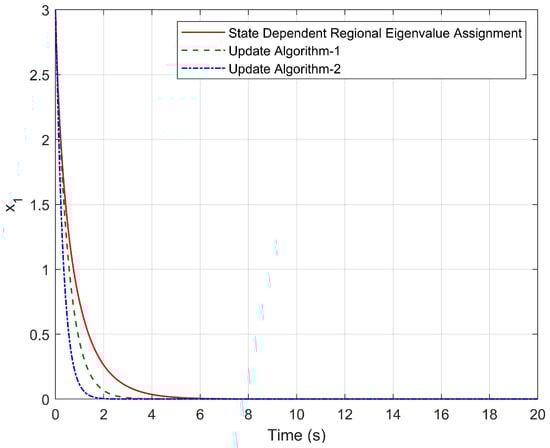
Figure 2.
Time response of for the initial condition , .
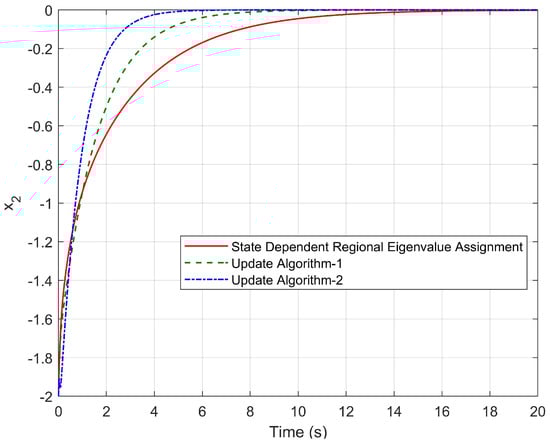
Figure 3.
Time response of for the initial condition , .
The changes in the locations of the pointwise eigenvalues during the simulation have been seen in Figure 4 when a fixed disc region is used. At the initial time, the eigenvalues are located in the place shown in black; at each time step, one of the eigenvalues follows the trajectory shown in blue, while the other eigenvalue follows the trajectory shown in green. The eigenvalues shown in red are the final eigenvalues at time . As can be seen, both eigenvalues move toward the real axis over time. After settling on the real axis, one of the eigenvalues move to the imaginary axis and the other moves away from that axis. To move all eigenvalues of the closed-loop system away from the imaginary axis, Update Algorithm 1 and Update Algorithm 2 can be used. Figure 5 and Figure 6 prove this statement by showing the eigenvalue trajectories.
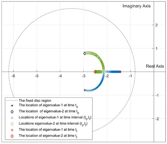
Figure 4.
Location of the closed-loop eigenvalues in the SDREAM-FDR (, ).
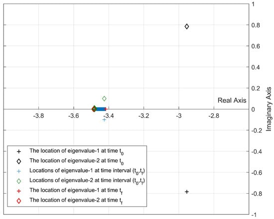
Figure 5.
Location of the closed-loop eigenvalues for Update Algorithm 1 (, ).
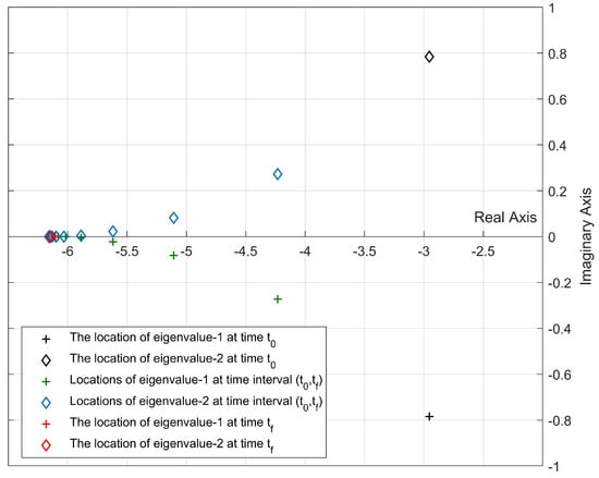
Figure 6.
Location of the closed-loop eigenvalues for Update Algorithm 2 (, ).
Figure 7 and Figure 8 reveal that both algorithms are capable of locating the pointwise eigenvalues in the desired discs whose parameters are updated by the rules given by Step 4 in Update Algorithm 1 and Step 5 in Update Algorithm 2.
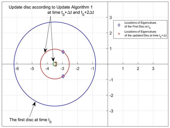
Figure 7.
Disc region and eigenvalue location samples for the Update Algorithm 1 (, ).
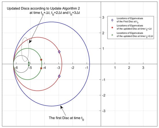
Figure 8.
Disc region and eigenvalue location samples for Update Algorithm 2 (, ).
The performance of the proposed algorithms are measured by using four performance criteria (Integral Time Absolute Error (ITAE), Integral Time Square Error (ITSE), Integral Absolute Error (IAE) and Integral Square Error (ISE)), which are mathematically expressed by
As seen in Table 1, the most effective control method is the control method using Update Algorithm 2. The similar results are obtained when the simulations run with different initial conditions were used. Figure 9 and Figure 10 represent the time responses of the state variables and for the initial condition , .

Table 1.
Performance Indices for the initial condition , .
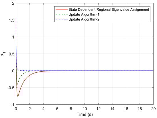
Figure 9.
Time response of for the initial condition , .
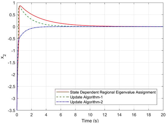
Figure 10.
Time response of for the initial condition , .
Considering the settling time and maximum overshoot, it is clear from Figure 9 and Figure 10 that Algorithm 2 is more capable of reducing the settling time than other algorithms. In addition, the hypothetical system exhibits no overshoot by means of Update Algorithm 2. In addition, from the comparison of the eigenvalue trajectories given in Figure 11, Figure 12 and Figure 13, it is found that the eigenvalues are forced to move away from the imaginary axis by using both Update Algorithm 1 and Update Algorithm 2. As a result, at each step time, the stability margin increases and the upper limit of the maximum overshoot value decreases. Figure 14 and Figure 15 also reveal that both algorithms are capable of locating the pointwise eigenvalues in the desired discs whose parameters are updated by the rules given by Step 4 in Update Algorithm 1 and Step 5 in Update Algorithm 2.
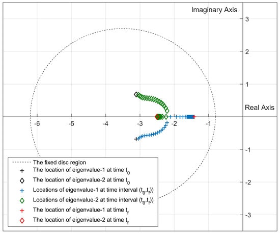
Figure 11.
Location of the closed-loop eigenvalues in the SDREAM-FDR (, ).
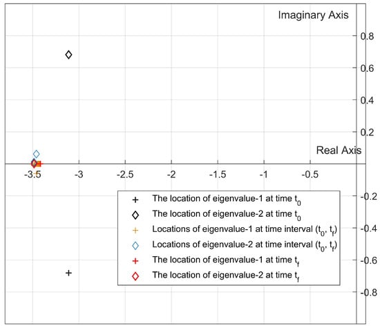
Figure 12.
Location of the closed-loop eigenvalues for Update Algorithm 1 (, ).
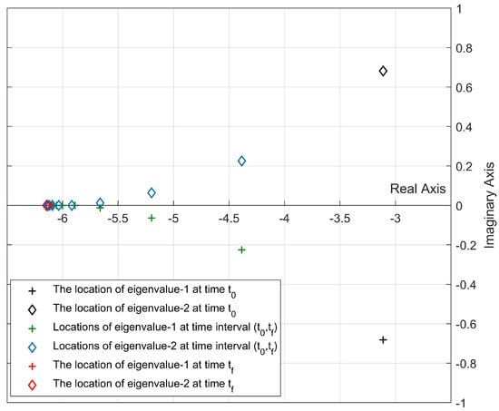
Figure 13.
Location of the closed-loop eigenvalues for Update Algorithm 2 (, ).
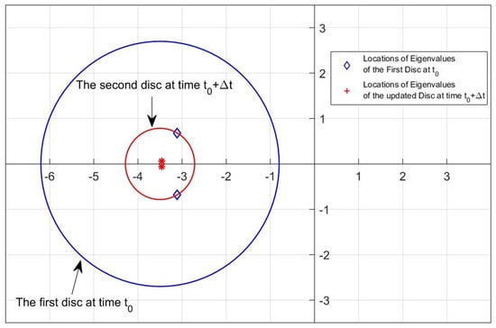
Figure 14.
Disc region and eigenvalue location samples for Update Algorithm 1 (, ).
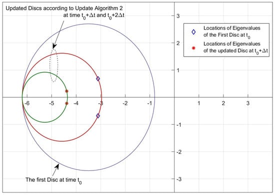
Figure 15.
Disc region and eigenvalue location samples for Update Algorithm 2 (, ).
Table 2 provides a comparison of the performance indices obtained from the simulation for the second initial condition. As expected, Update Algorithm 2 shows the most effective performance.
Table 2.
Performance Indices for the initial condition , .
4. Application
In this section, Update Algorithm 1 and Update Algorithm 2 are applied to a three-DOF helicopter experimental setup to show the effectiveness of the proposed methods. This platform is a widely used experimental setup to determine the performance of proposed controller designs [34,35,36,37,38,39,40,41]. First, the mathematical model of the three-DOF helicopter is presented, and then, its SDC formulation required to design the state feedback control law is given. Secondly, a set of simulations is conducted to compare the effectiveness of the update algorithms for SDREAM with that of SDREAM with the fixed disc region (SDREAM-FDR). Finally, the operations performed in the simulations were tested, and the experimental results were examined.
4.1. Mathematical Model of the 3-DOF Helicopter
The three-DOF helicopter experimental setup represented in Figure 16 is produced by Quanser Inc. to test the developed control algorithms. This setup, designed similar to a tandem rotor helicopter, is a multiple input–multi output (MIMO) system and has some nonlinear dynamic behaviour.
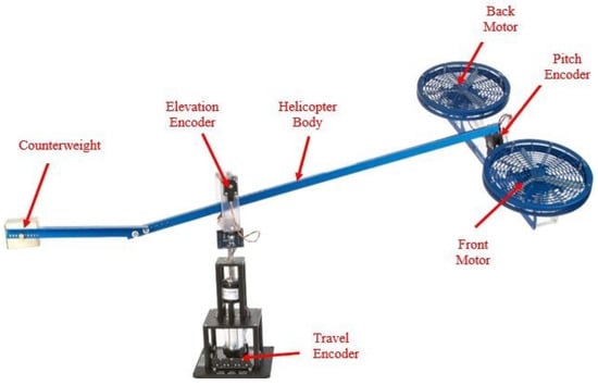
Figure 16.
Three-DOF Helicopter Experimental Setup.
Three-DOF helicopter has three free rotation motion about three axes named as elevation, pitch and travel, as shown in Figure 17. The attitude of the three-DOF helicopter is measured with the help of three sensors (encoders). The controller inputs given to the system are provided by the propellers, each driven by a DC motor, whose axes are parallel to each other. A counterweight is placed at the other end of the system to change the effective mass of the helicopter. This setting is adjusted by mounting the counterweight at different positions on the helicopter body. Thus, it helps reduce the required loads on the motors while controlling the system. Although the system has three degrees of freedom, only two motors are installed for the purpose of controlling it in 3-dimensional space. Therefore, the experimental setup is an under-actuated system and is allowed to track the reference trajectories defined in only two axes. In this study, the reference trajectories are designed in the elevation and travel axes.
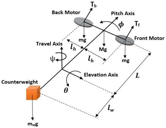
Figure 17.
Free-body diagram of 3-DOF Helicopter.
A simplified nonlinear model was derived in [42] shown below.
where and , respectively, denote the cyclic thrust force and the collective thrust force which are altered to control the elevation , pitch and travel angles. The first three equations are Euler’s equations for describing the rotational motions in 3-D space. The last two first-order differential equations represent the motor dynamics relating to the changes in the trust forces to the changes in the back and front motor voltages ( and ). The units of the variables in the model are listed in Table 3.
Table 3.
Units of variables.
The Comprehensive Identification from Frequency Responses (CIFER) program, a well-known parameter identification program, was used to obtain the parameters of the nonlinear three-DOF helicopter model in the study of [42]. The parameters of the nonlinear helicopter model, have been previously estimated in the study of [42], were used in this study and are given in Table 4.
Table 4.
Parameter Values of the Three-DOF Helicopter Model.
The state vector is defined as
and used to transform the helicopter model in Equation (50) into the state-space model
and the control input vector u is defined as
4.2. Controller Design
The state-space model in Equation (52) is rewritten in the factorised form using the extended linearisation technique, and the SDC matrices are selected as
and
where , , and .
The control law is designed to track the step commands in the elevation () and travel () axes of helicopter. Therefore, to achieve the desired position of the helicopter in elevation and travel axes, the factorised SDC system is augmented as follows:
Given the output vector as , where the output matrix C is selected to be
and the error vector is composed of
and , then the augmentation of the states x yields the following error dynamics
where
Therefore, the control law is replaced with
to ensure . Here, is the controller gain matrix for the augmented system. After the augmentation, the increase in the number of eigenvalues to be placed in a desired disc region is equal to the number of state variables that are augmented. Therefore, the number of eigenvalues to be placed within a disc region for a three-DOF helicopter increases from eight to ten due to the reference tracking in the travel and elevation axis.
4.3. Simulation Results
In the simulations, the augmented three-DOF helicopter model (56) is used. The initial elevation, pitch and travel angular positions of the helicopter are set to , and , respectively. Each simulation lasts for 70 s. The desired elevation command is during the whole simulation time, and the desired travel command is set to be for the first 30 s, then for the following 40 s. Q and R are used in all simulation studies. Q and R are selected by
and . The initial disc region of each simulation is the same, and the sampling time () of each simulation is 0.01 s. The initial disc centre and radius are, respectively, selected to be −2 () and 1.8 ().
In the SDREAM-FDR, these disc parameters remain unchanged during the simulations, whereas they are changed depending on the closed-loop system eigenvalues in the simulations where the update algorithms are utilised. In Update Algorithm 1, the centre is fixed and the radius is updated according to the locations of the pointwise eigenvalues, whereas both disc parameters are updated at each time instant in Update Algorithm 2. Therefore, the most important results that should be analysed in this section whether the pointwise eigenvalues can be placed in the desired disc regions by using the updated algorithms successfully or not.
Figure 18, Figure 19 and Figure 20 show the movement of the pointwise eigenvalues during the simulation. As can be seen from the figures, the locations of the eigenvalues change at each time step from the initial time step () to the final time step (). In the figures, the red square and blue cross marker illustrate the eigenvalues at the initial time and at the final time, respectively. The locations of the eigenvalues that move within the time interval (, ) are shown with grey plus markers. From the figures, it is apparent that the pointwise eigenvalues move further away from imaginary axis and closer to the real axis at each time instant if Update Algorithm 2 is used to design the controller.
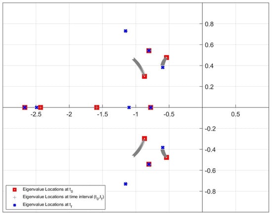
Figure 18.
Location of the closed-loop eigenvalues in the SDREAM-FDR in the simulation.
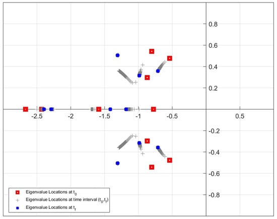
Figure 19.
Location of the closed-loop eigenvalues for Update Algorithm 1 in the simulation.
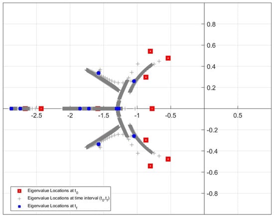
Figure 20.
Location of the closed-loop eigenvalues for Update Algorithm 2 in the simulation.
Figure 21 and Figure 22 are given for a better understanding of the update algorithms. It is really difficult to show the locations of all pointwise eigenvalues at each time instant in one plot because one experiment includes approximately 7000 sets of the pointwise eigenvalues and each set has 10 eigenvalues. To make it more understandable to the readers, several time instants are arbitrarily selected, and the figures showing the locations of the pointwise eigenvalues are plotted for only these time instants. The selected time instants are 0, 0.01, 0.02 and 0.03 s for both the updated algorithms. Figure 21 and Figure 22 show that both algorithms are able to place the pointwise eigenvalues in the desired discs updated by the rules given by Step 4 in Update Algorithm 1 and Step 5 in Update Algorithm 2.
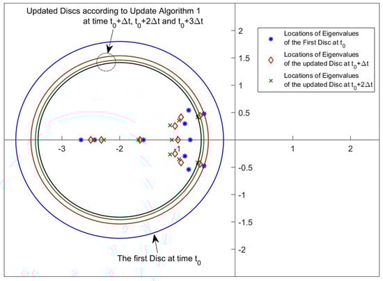
Figure 21.
Disc region and eigenvalue location samples for Update Algorithm 1 in the simulation.
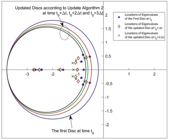
Figure 22.
Disc region and eigenvalue location samples for Update Algorithm 2 in the simulation.
Figure 23 shows that the elevation motion of three-DOF helicopter controlled by two proposed update algorithms and SDREAM-FDR. From Figure 23, it is seen that the steady-state error does not occur for three algorithms. In addition, the minimum settling time is obtained by using Update Algorithm 2. Figure 24 shows that the travel responses of the helicopter is controlled by three different approaches. As can be seen from the figures, the best response on travel axis can be achieved by using Update Algorithm 2. As a result, the settling time and maximum overshoot can be reduced by using the update algorithms.
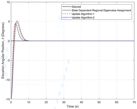
Figure 23.
Elevation response of the helicopter controlled by three different approaches in simulations.
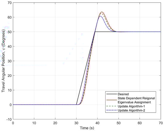
Figure 24.
Travel response of the helicopter controlled by three different approaches in simulations.
The last result in this section is the comparison of three different algorithms based on their performance criteria. Table 5 shows that the most appropriate approach according to the performance criteria is Update Algorithm 2.
Table 5.
Performance Indices for simulation studies.
4.4. Experimental Results
This section contains the experimental study results. Each experiment is performed with the strategy in the previous section. Therefore, in all experiments, the controller parameters, the trajectory to be followed, and the selected initial disc region (centre and radius) are kept the same as those used in the simulations.
Due to the large size of data sets, Figure 25, Figure 26 and Figure 27 are produced in order to show the movement of eigenvalues more clearly. The initial and final locations of the eigenvalues are shown with red square and blue cross markers. In addition, the grey plus markers represent the eigenvalue locations that change at each time step in time interval (,). As can be seen from the figures, Update Algorithm 2 moves the eigenvalues further away from the imaginary axis and closer to the real axis compared to other methods, similarly to the results in the simulation studies. Accordingly, the system responses can be improved in a manner that the maximum overshoot value decreases and the settling time is shortened.
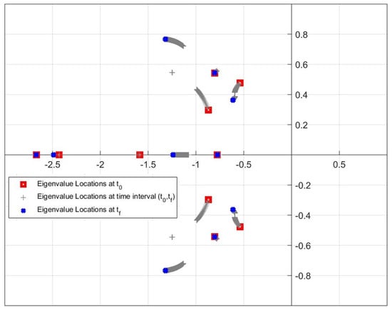
Figure 25.
Motion of the location of the closed-loop eigenvalues in the SDREAM-FDR.
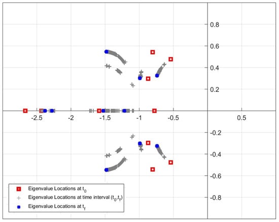
Figure 26.
Motion of the location of the closed-loop eigenvalues for Update Algorithm 1.
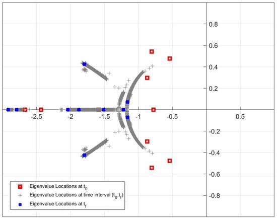
Figure 27.
Motion of the location of the closed-loop eigenvalues for Update Algorithm 2.
Figure 28 and Figure 29 reveal that both algorithms are capable of placing the pointwise eigenvalues in the desired discs whose parameters are updated by the rules given by Step 4 in Update Algorithm 1 and Step 5 in Update Algorithm 2. Similarly to the simulation results, the time instants of 0, 0.01, 0.02 and 0.03 s are chosen again and the figures are generated only for these time instants.
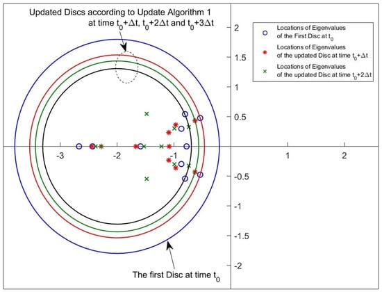
Figure 28.
Disc region and eigenvalue location samples for Update Algorithm 1.
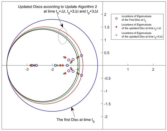
Figure 29.
Disc region and eigenvalue location samples for Update Algorithm 2.
To examine the effects of the updated locations of the pointwise eigenvalues on the transient response characteristics of the system, a time response analysis is performed. Figure 30 shows the elevation motions of the helicopter controlled by two proposed update algorithms and SDREAM-FDR. From Figure 30, it is seen that three algorithms are effective in keeping the helicopter at the zero desired elevation, and no overshoot is observed. In addition, the almost zero error in the elevation response is achieved within 10 s by Update Algorithm 2, which yields the minimum settling time. However, the almost zero error in the elevation response is achieved within 20 s by SDREAM-FDR, and this figure is the maximum settling time amongst the others. On the other hand, some minor oscillations occur in the elevation axis when the desired travel command is given to the system. However, these oscillations due to the travel command are suppressed rapidly.
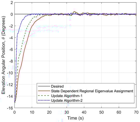
Figure 30.
Elevation response of the helicopter controlled by three different approaches.
The travel responses of the helicopter controlled by three different approaches are shown in Figure 31. As can be seen from the results, the best travel axis system response is obtained with Update Algorithm 2. The results coincide with the idea of developing algorithms. Update Algorithm 2 reduces both the settling time and maximum overshoot in the system response compared to the other two approaches. The system response with Update Algorithm 1 also has a better settling time and maximum overshoot than those with SDREAM-FDR. Although the underactuated system limits the improvement of the system response in the travel axis, it is experimentally seen that the proposed algorithms are effective.
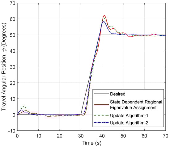
Figure 31.
Travel response of the helicopter controlled by three different approaches.
Figure 32 shows the final axis, namely, pitch motion. Although there is no reference tracking on the pitch axis, regulation is made for both the travel axis and the elevation axis control. The pitch axis is also limited to 90 degrees due to the structure of the experimental setup, and this value should never be reached. As can be seen from Figure 32, the smoothest system response and the least oscillation are obtained by updating the centre and radius of the disc at each time step, that is, by using Update Algorithm 2.
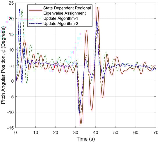
Figure 32.
Pitch response of the helicopter controlled by three different approaches.
The controller gains () are given in Figure 33, Figure 34 and Figure 35. Update Algorithm 2 produces more significant changes in the controller gains than the other approaches, especially within 10 s. The reason is that it requires more control effort to meet the control requirements within 10 s. This effect can be also observed in Figure 36 and Figure 37, which represent the changes in the voltage values of the front and back motor inputs over time.
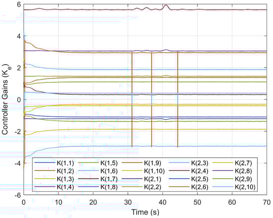
Figure 33.
Controller gains of the SDREAM-FDR.
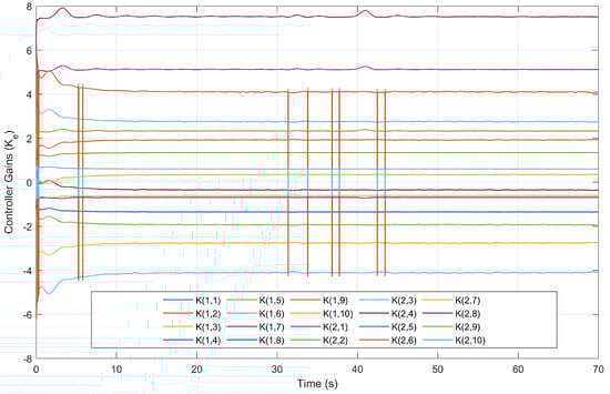
Figure 34.
Controller gains of the approach using Update Algorithm 1.
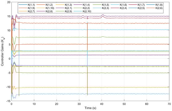
Figure 35.
Controller gains of the approach using Update Algorithm 2.
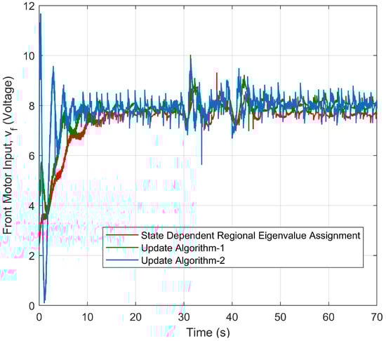
Figure 36.
Front motor input of the helicopter controlled by three different approaches.
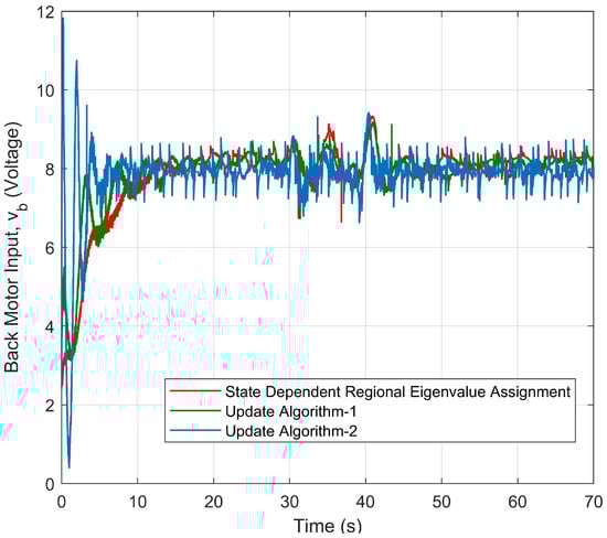
Figure 37.
Back motor input of the helicopter controlled by three different approaches.
In order to compare the performances of three different approaches in transient responses, performance indices were calculated. As can be seen from Table 6, the most appropriate approach according to the performance criteria is the one in which Update Algorithm 2 is used.
Table 6.
Performance indices for experimental studies.
5. Conclusions
The aim of this study was to extend a theory about the regional eigenvalue assignment developed for linear systems to nonlinear systems. In addition, to improve the transient responses, two update algorithms are introduced in this study as well. In the first proposed algorithm, the disc centre is kept constant and the radius is reduced over time, while in the second algorithm, the radius is reduced and, at the same time, the disc center is shifted to the left in the complex plane. Then, a state feedback control law is derived to place all pointwise eigenvalues of the “frozen” closed-loop system in the desired disc region updated at each time instant. The proposed algorithms were tested in simulations and implemented into the three-DOF laboratory helicopter. In simulations, a hypothetical second-order nonlinear system was employed to demonstrate the effectiveness of algorithms using two different initial conditions. The results of simulations and experiments verify the effectiveness of update algorithms for nonlinear systems by comparing SDREAM using the update algorithms with SDREAM-FRD. From the results, it is found that the system responses can be improved by using these update algorithms since both algorithms help reduce the settling times and maximum overshoot. The stability margin and damping ratio can be improved more successfully with Update Algorithm 2 than other methods in exchange for slightly a higher control effort during the initial phase of the experiments. In addition, the benchmarking results using ISE, IAE, ITAE and ITSE performance criteria have shown that Update Algorithm 2 is more effective than Update Algorithm 1 and SDREAM-FDR.
Author Contributions
Conceptualization: A.Ç.A., E.H.Ç., G.I. and M.U.S.; methodology: A.Ç.A., E.H.Ç., G.I. and M.U.S.; software: A.Ç.A.; validation: A.Ç.A., E.H.Ç., G.I. and M.U.S.; investigation: A.Ç.A., E.H.Ç., G.I. and M.U.S.; resources: A.Ç.A., E.H.Ç., G.I. and M.U.S.; writing—original draft preparation: A.Ç.A. and E.H.Ç.; writing—review and editing: A.Ç.A., E.H.Ç., G.I. and M.U.S.; visualization: A.Ç.A. and E.H.Ç.; supervision: M.U.S. and G.I. All authors have read and agreed to the published version of the manuscript.
Funding
This research received no external funding.
Conflicts of Interest
The authors declare no conflict of interest.
References
- Lee, C.H.; Shin, M.H.; Chung, M.J. A design of gain-scheduled control for a linear parameter varying system: An application to flight control. Control Eng. Pract. 2001, 9, 11–21. [Google Scholar] [CrossRef]
- Ma, T. Eigenvalue assignment enabled control law for multivariable nonlinear systems with mismatched uncertainties. Eur. J. Control 2020, 56, 154–166. [Google Scholar] [CrossRef]
- Yi, S.; Nelson, P.W.; Ulsoy, A.G. Proportional-Integral Control of First-Order Time-Delay Systems via Eigenvalue Assignment. IEEE Trans. Control Syst. Technol. 2013, 21, 1586–1594. [Google Scholar]
- Carotenuto, L.; Franzé, G. A general formula for eigenvalue assignment by static output feedback with application to robust design. Syst. Control Lett. 2003, 49, 175–190. [Google Scholar] [CrossRef]
- Koru, A.T.; Sarsılmaz, S.B.; Yucelen, T.; Muse, J.A.; Lewis, F.L.; Açıkmeşe, B. Regional Eigenvalue Assignment in Cooperative Linear Output Regulation. IEEE Trans. Autom. Control 2023, 68, 4265–4272. [Google Scholar] [CrossRef]
- Haddad, W.M.; Bernstein, D.S. Controller design with regional pole constraints. IEEE Trans. Autom. Control 1992, 37, 54–69. [Google Scholar] [CrossRef]
- Furuta, K.; Kim, S. Pole assignment in a specified disk. IEEE Trans. Autom. Control 1987, 32, 423–427. [Google Scholar] [CrossRef]
- Yaz, E.; Skelton, R.; Grigoriadis, K. Robust regional pole assignment with output feedback. In Proceedings of the 32nd IEEE Conference on Decision and Control, San Antonio, TX, USA, 15–17 December 1993. [Google Scholar]
- Garcia, G.; Bernussour, J. Pole assignment for uncertain systems in a specified disk by state feedback. IEEE Trans. Autom. Control 1995, 40, 184–190. [Google Scholar] [CrossRef]
- Garcia, G.; Daafouz, J.; Bernussour, J. Output feedback disk pole assignment for systems with positive real uncertainty. IEEE Trans. Autom. Control 1996, 41, 1385–1391. [Google Scholar] [CrossRef]
- Kim, H.S.; Han, H.S.; Lee, J.G. Pole placement of uncertain discrete systems in the smallest disk by state feedback. In Proceedings of the 35th IEEE Conference on Decision and Control, Kobe, Japan, 13 December 1996. [Google Scholar]
- Chou, J.-H. Pole-assignment robustness in a specified disk. Syst. Control Lett. 1991, 16, 41–44. [Google Scholar] [CrossRef]
- Schuchert, P.; Karimi, A. A convex set of robust D—Stabilizing controllers using Cauchy’s argument principle. IFAC-PapersOnLine 2022, 55, 49–54. [Google Scholar] [CrossRef]
- Ling, B. State-feedback regional pole placement via LMI optimization. In Proceedings of the 2001 American Control Conference, Arlington, VA, USA, 25–27 June 2001. [Google Scholar]
- Soliman, H.; Dabroum, A.; Mahmoud, M.; Soliman, M. Guaranteed-cost reliable control with regional pole placement of a power system. J. Frankl. Inst. 2011, 348, 884–898. [Google Scholar] [CrossRef]
- Wisniewski, V.; Maddalena, E.; Godoy, R. Discrete-time regional pole-placement using convex approximations: Theory and application to a boost converter. J. Control Eng. Pract. 2019, 91, 104102. [Google Scholar] [CrossRef]
- Almeida, M.O.; Araújo, J.M. Partial Eigenvalue Assignment for LTI Systems with D-Stability and LMI. J. Control Autom. Electr. Syst. 2019, 30, 301–310. [Google Scholar] [CrossRef]
- Baker, W.A.; Schneider, S.C.; Yaz, E.E. Robust regional eigenvalue assignment by dynamic state-feedback control for nonlinear continuous-time systems. In Proceedings of the 2015 54th IEEE Conference on Decision and Control (CDC), Osaka, Japan, 15–18 December 2015. [Google Scholar]
- Xiong, S.; Chen, M.; Wei, Z. Tracking flight control of UAV based on multiple regions pole assignment method. Aerosp. Sci. Technol. 2022, 129, 107848. [Google Scholar] [CrossRef]
- Chilali, M.; Gahinet, P.; Apkarian, P. Robust pole placement in LMI regions. IEEE Trans. Autom. Control 1999, 44, 2257–2270. [Google Scholar] [CrossRef]
- Leite, V.J.; Peres, P.L. An improved LMI condition for robust D-stability of uncertain polytopic systems. IEEE Trans. Autom. Control 2003, 48, 500–504. [Google Scholar] [CrossRef]
- Satoh, A.; Sugimoto, K. An LMI approach to gain parameter design for regional eigenvalue/eigenstructure assignment. In Proceedings of the 45th IEEE Conference on Decision and Control, San Diego, CA, USA, 13–15 December 2006. [Google Scholar]
- Sahoo, P.R.; Goyal, J.K.; Ghosh, S.; Naskar, A.K. New results on restricted static output feedback controller design with regional pole placement. IET Control Theory Appl. 2019, 13, 1095–1104. [Google Scholar] [CrossRef]
- Richiedei, D.; Tamellin, I. Active control of linear vibrating systems for antiresonance assignment with regional pole placement. J. Sound Vib. 2021, 494, 115858. [Google Scholar] [CrossRef]
- Zhai, J.; Gao, L.; Li, S. Robust pole assignment in a specified union region using harmony search algorithm. Neurocomputing 2015, 155, 12–21. [Google Scholar] [CrossRef]
- Rosinová, D.; Veselý, V.; Hypiusová, M. Novel robust gain scheduled PID controller design using DR regions. Asian J. Control 2021, 24, 2062–2073. [Google Scholar] [CrossRef]
- Veselý, V.; Körösi, L. Robust PI-D Controller Design for Uncertain Linear Polytopic Systems Using LMI Regions and H2 Performance. IEEE Trans. Ind. Appl. 2019, 55, 5353–5359. [Google Scholar] [CrossRef]
- Singh, H.; Naidu, D.S.; Moore, K.L. On regional pole assignment in discrete-time systems using linear quadratic regulator theory. In Proceedings of the 1994 American Control Conference—ACC ’94, Baltimore, MD, USA, 29 June–1 July 1994. [Google Scholar]
- Mori, Y.; Shimemura, Y. On a design method for feedback control law to locate the eigenvalues in a specified region. SICE 1980, 16, 462–463. [Google Scholar]
- Bogachev, A.V.; Grigorev, V.V.; Drozdov, V.N.; Korovyakov, A.N. Analytic design of controls from root indicators. Autom. Remote Control 1979, 40, 1118–1123. [Google Scholar]
- Arıcan, A.Ç.; Çopur, E.H.; Inalhan, G.; Salamci, M.U. State Dependent Regional Pole Assignment Controller Design for a 3-DOF Helicopter Model. In Proceedings of the 2023 International Conference on Unmanned Aircraft Systems (ICUAS), Warsaw, Poland, 6–9 June 2023. [Google Scholar]
- Arıcan, A.Ç.; Çopur, E.H.; Inalhan, G.; Salamci, M.U. Sliding Mode Control of a 3-DOF Helicopter with State Dependent Regional Pole Placement. In Proceedings of the 2023 24th International Carpathian Control Conference (ICCC), Miskolc-Szilvásvárad, Hungary, 27–30 May 2023. [Google Scholar]
- Cimen, T. Systematic and effective design of nonlinear feedback controllers via the state-dependent Riccati equation (SDRE) method. Ann. Rev. Control 2010, 34, 32–51. [Google Scholar] [CrossRef]
- Ozcan, S.; Çopur, E.H.; Arican, A.C.; Salamci, M.U. A Modified SDRE-based Sub-optimal Hypersurface Design in SMC. IFAC-PapersOnLine 2020, 53, 6250–6255. [Google Scholar] [CrossRef]
- Copur, E.H.; Arican, A.C.; Ozcan, S.; Salamci, M.U. An update algorithm design using moving Region of Attraction for SDRE based control law. J. Frankl. Inst. 2019, 356, 8388–8413. [Google Scholar] [CrossRef]
- Kocagil, B.M.; Ozcan, S.; Arican, A.C.; Guzey, U.M.; Copur, E.H.; Salamci, M.U. MRAC of a 3-DoF Helicopter with Nonlinear Reference Model. In Proceedings of the 2018 26th Mediterranean Conference on Control and Automation (MED), Zadar, Croatia, 19–22 June 2018. [Google Scholar]
- Arıcan, A.Ç.; Ozcan, S.; Kocagil, B.M.; Guzey, Ü.M.; Salamci, M.U. Suboptimal control of a 3 dof helicopter with state dependent riccati Equations. In Proceedings of the XXVI International Conference on Information, Communication and Automation Technologies (ICAT), Sarajevo, Bosnia and Herzegovina, 26–28 October 2017. [Google Scholar]
- Kara, F.; Salamci, M.U. Controller Design for a Nonlinear 3 DOF Helicopter Model Using Adaptive Sliding Surfaces. In Proceedings of the 2019 XXVII International Conference on Information, Communication and Automation Technologies (ICAT), Sarajevo, Bosnia and Herzegovina, 20–23 October 2019. [Google Scholar]
- Perk, B.E.; Inalhan, G. Safe Motion Planning and Learning for Unmanned Aerial Systems. Aerospace 2022, 9, 56. [Google Scholar] [CrossRef]
- Chaoui, H.; Yadav, S.; Ahmadi, R.S.; Bouzid, A.E.M. Adaptive Interval Type-2 Fuzzy Logic Control of a Three Degree-of-Freedom Helicopter. Robotics 2020, 9, 59. [Google Scholar] [CrossRef]
- Peng, H.; Wei, L.; Zhu, X.; Xu, W.; Zhang, S. Aggressive maneuver oriented integrated fault-tolerant control of a 3-DOF helicopter with experimental validation. Aerosp. Sci. Technol. 2022, 120, 107265. [Google Scholar] [CrossRef]
- Ishutkina, M. Design and Implimentation of a Supervisory Safety Controller for a 3DOF Helicopter. Master’s Thesis, Massachusetts Institute of Technology, Cambridge, MA, USA, 2004. [Google Scholar]
Disclaimer/Publisher’s Note: The statements, opinions and data contained in all publications are solely those of the individual author(s) and contributor(s) and not of MDPI and/or the editor(s). MDPI and/or the editor(s) disclaim responsibility for any injury to people or property resulting from any ideas, methods, instructions or products referred to in the content. |
© 2023 by the authors. Licensee MDPI, Basel, Switzerland. This article is an open access article distributed under the terms and conditions of the Creative Commons Attribution (CC BY) license (https://creativecommons.org/licenses/by/4.0/).