Experimental and Numerical Modal Analysis of a Composite Rocket Structure

Abstract

Finite Element Analysis (FEA) is a powerful tool that can aid in the engineering design process to reduce cost and time. However, it is best used in conjunction with experimental data, through which its numerical results can be verified. This paper presents the experimental and numerical modal analyses of an experimental rocket aerostructure to verify the accuracy of the numerical models. This aerostructure has been through flight loads and a recovery. The first numerical results for the rocket showed a 96% difference with the experimental ones. Subsequently, three mass refinements were made to create calibrated FEM models whose results differed from the experimental ones by 19% to 8%. Additionally, as expected, the FEM results tended to overestimate the stiffness of structures. The numerical simulations for all components were performed through ANSYS software, and the experiments were conducted using the hammer tap test with laser vibrometers as sensors.

1. Introduction

Rocket design is a complex process that encompasses many fields of technology and engineering. The design process includes disciplines such as aerodynamics, structural analysis, avionics, recovery, payload, and systems engineering. These areas can then be subdivided into specialized focuses. For example, structural design involves load analysis, material selection, manufacturing, etc. Further, these subdivisions can be broken down again, which makes rocket design a complex and expensive process. Therefore, to simplify this procedure, it is imperative to reliably use tools such as Finite Element Analysis to aid in the design process. This allows for new designs to be tested to ensure they survive under their intended load conditions and helps to locate any potential defects. However, to achieve proper results, the FEA process is very reliant on the user input being accurate to real-world conditions. The user must ensure that parameters such as geometry, material properties, boundary conditions, meshing, and load application are as close to the real conditions as possible. Therefore, it is very important to verify the numerical results through experiments to confirm the model’s accuracy.

The purpose of the present study is to conduct the numerical modal analysis of three separate components of a composite experimental rocket, designed and built by the Toronto Metropolitan University (TMU) rocketry club, and then verify these results through experimental means. This aerostructure has been through flight loads and a recovery. TMU Rocketry is an award-winning design team that designs, builds, and launches high-powered competition rockets. The numerical results obtained through FEA can then be verified through experimental data. This approach provides two sets of outcomes, the first outcome is that the results will help define the vibrational characteristics of the structure. Modal analysis is the first step in conducting a vibrational analysis; it also provides important information such as the natural frequencies and modes shapes of the structure. The second outcome is that the results will help to verify the correctness and precision of the FEA modeling. The results can also support the investigation into any potential discrepancies and sources of errors that can then be addressed. The latter outcome is especially important, as adjustments could subsequently be made to create a more accurate FEM model. It is expected that the resulting so-called calibrated FEM model can then be used to ultimately determine whether the structure satisfies its design criteria for any set of intended loading and working conditions.

2. Literature Review

From launch to recovery, a rocket aerostructure experiences static and dynamic loads that must be analyzed to ensure a successful flight. The rocket must be able to survive loadings such as buckling, inertial loads, and vibrations. The following brief literature review explores the background required for such analysis as well as various examples.

A few studies were found where experiments involving composite components were conducted. A comprehensive study performed by Chinta et al. [1] involved a modal analysis on composite plates with varying fiber orientations. The results were then compared with those obtained for the corresponding beams between FEM and Classical Lamination Theory (CLT). The other studies cited here conducted both FEA and experiments to gather and compare these results. The majority of these studies involved cylindrical shells or fuselages. A study conducted by Blom et al. [2] consisted of the modal testing of a composite cylinder with circumferentially varying stiffness using a shaker test. Another study, conducted by Simsiriwong and Sullivan [3], utilized a shaker test to obtain experimental results for a composite airframe. Similarly, studies by others also utilized the same process but slightly differed in their equipment and methodologies. A study concerning the modal analysis of a large fuselage model conducted by NASA [4] utilized impact testing, where their measurements were performed using both accelerometers and Laser Doppler Vibrometers (LDVs) depending on the stage of assembly. Other studies featuring smaller models have utilized the hammer impact test (TAP testing) for excitation. Cosco et al. [5] conducted a study looking at the experimental characterization for torsional damping in CFRP disks utilizing the TAP test.

As mentioned earlier, the objectives of this paper are to conduct the numerical simulation and modal analysis of the components of an experimental composite rocket and then verify these results through experimental means. Based on the comparison between the modal analysis data attained experimentally and the numerical results obtained from the FEM-based modeling, adjustments are subsequently made to create more accurate calibrated FEM models.

2.1. Finite Element Analysis

The Finite Element Method (FEM) is a powerful tool for analysis. The study presented here consists of two main areas, composite modeling and modal analysis. The first is completed through the ANSYS ACP workflow due to the composite nature of the model. The second is completed through the modal workflow [6].

2.1.1. Composite Modeling

One of the most utilized theories for modeling composite shells is the First-Order Shear Deformation Theory (FSDT). Following the explanation provided in “Finite Element Analysis of Composite Materials Using Ansys” by Ever J. Barbero [7], FSDT is based on the following assumptions:

• If a straight line is drawn through the thickness of the shell while it is undeformed, then it must remain straight when the shell is deformed. The angles it forms (if any) with the normal to the undeformed mid-surface are denoted by ϕ_x and ϕ_y when measured in the xz and yz planes, respectively.
• As the shell deforms, the change in thickness is negligible.

These assumptions have been verified through experimental observations in a majority of laminate shells under certain conditions. First, the aspect ratio, which is defined as a ratio between the shortest surface dimension and the thickness, must be larger than 10. Second, the stiffness of the laminas in shell coordinates (x, y, z) must not differ by more than two orders of magnitude. In this case, the composite structure being analyzed passes all these requirements and assumptions [8]. These assumptions and conditions were also explored in a study conducted by Raciti et al. [9], which utilized the Classical Laminated Plate Theory (CLPT) and FDST for the vibrational analysis of composite beams. Their results showed that for thick laminates, these theories were adequate for predicting the behavior.

The composite modeling of the structure is conducted through ANSYS ACP. In terms of meshing, Ansys offers two main options for elements: SHELL181 and SHELL281. Both of these options are well suited for applications such as the present study and are utilized for analyzing thin to moderately thick shell structures. The only difference between the two elements is their respective numbers of nodes and degrees of freedom. The SHELL181 element has four nodes with six degrees of freedom per node (translations and rotations at x, y, and z), whereas SHELL281 has eight nodes in total. The element chosen usually depends on a few factors such as the computational resources available or the amount of resolution required [8]. It should be noted that there are also other elements and approaches that can be utilized. In a study performed by Maiti and Sinha [10], an investigation was conducted to develop a nine-noded isoparametric element to accurately determine bending and free vibration behavior in composite beams. This study also analyzed the effects of various parameters (fiber orientation, ply thickness, stacking sequence, etc.) on stresses, strains, and natural frequencies. Additionally, in a study conducted by Jun et al. [11], the free vibration and buckling behaviors of axially loaded composite beams were investigated using the dynamic stiffness method.

2.1.2. Modal Analysis

Calculating the modal response of a system is a very important step towards determining its dynamic response. However, it should be clarified that the modal analysis does not actually calculate the stress and strain of the structure; instead, it calculates the vibrational characteristics (i.e., natural frequencies and mode shapes). The analysis also helps the structure avoid resonant frequencies and gives an idea of how the design will react to various dynamic loads [7,8].

The linear equation of motion for free, undamped vibration can be described as:

$$\left[M\right]\ddot{u}+\left[K\right]u=\left\{0\right\},$$

(1)

where [M] is the mass matrix and [K] is the stiffness matrix. Assuming harmonic motion results in the following eigenvalue equation below:

$$\left(\left[K\right]-{\omega }_i^2\left[M\right]\right){\left\{\phi \right\}}_i=\left\{0\right\},$$

(2)

This equality can be solved in two ways. The first is if ${\left\{\phi \right\}}_i=\left\{0\right\}$, this is a trivial solution and implies no vibration. The non-trivial solution is found by setting the determinant of the eigenvalue equation equal to zero. This problem can be solved for n roots $({\omega }_1^2,{\omega }_2^2,\dots {\omega }_n^2$), where n is the total number of degrees of freedom in the system. The roots themselves represent the eigenvalues of the equation. Additionally, for the eigenvalue there is also a corresponding eigenvector ${\left\{\phi \right\}}_1, {\left\{\phi \right\}}_2, \dots {\left\{\phi \right\}}_n$. The structure’s natural circular frequencies, ${\omega }_i$, can be turned into natural frequencies in Hz [6,12].

$$f_i=\frac{{\omega }_i}{2\pi }$$

(3)

Finally, the eigenvectors themselves represent the mode shapes of the structure. Mode shapes are the shape assumed by the structure when vibrating at frequency, $f_i$.

3. Setup

The experimental modal analysis of the rocket aerostructure will be carried out using the hammer impact test (TAP testing), and measurements will be made using a laser vibrometer. This section will briefly cover the setups for both the numerical and experimental analyses. On the numerical side, this includes details about the CAD geometry, material specifications, loads, boundary conditions, and meshing. The experimental setup will discuss the vibrometry instruments, equipment, and the setup configurations for the different tests.

3.1. Numerical Analysis Setup

As stated in Section 2.1, the simulations for each model were conducted in Ansys Workbench. The process for the analyses was a combination of both Ansys ACP (Pre) and modal workflows.

3.1.1. CAD Model

A complete solid assembly CAD model of the one-stage rocket aerostructure was provided by the MetRocketry Design Team (MDT). The solid body CAD of the one-stage rocket was modified to accurately reflect the actual aerostructure, as the experimental test piece only consisted of the assembled booster section. This process involved removing all unnecessary internal components from the model. The only components that were kept for the analysis were the booster tube, boat tail–booster coupler, centering rings, bulkhead, boat tail, and the fins. Additionally, the geometry was converted to an entirely surface model to prepare the model for composite layup in Ansys ACP. 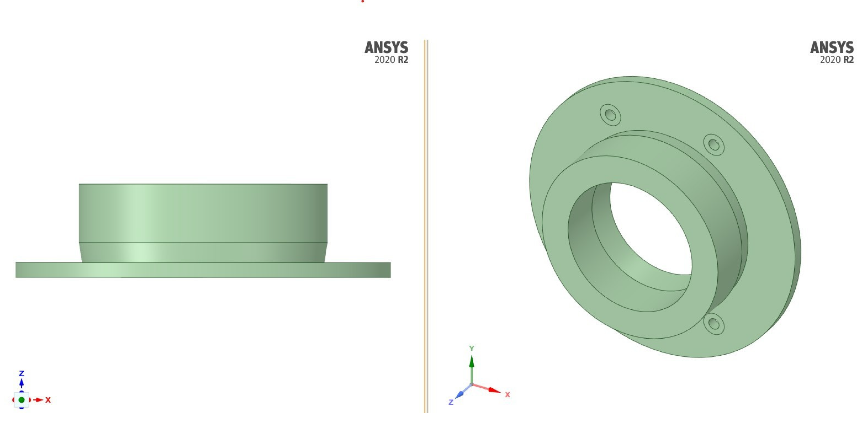Figure 1 provides the rocket aerostructure surface model. To secure the rocket to the support table, a circular support structure was required (see Figure 2).

To ensure accuracy between the experiment and the numerical simulations, the support model was also included with the rocket geometry.

3.1.2. Material and Layup Details

As the airframe and its components are completely manufactured from composites, this section provides details into their materials and ply layup. The airframe structure is manufactured via a light filament wounding process. Its laminate is four layers of carbon fiber using a [45/10/10/45] layup. The couplers are also manufactured using filament winding and use a [45/−45/45/−45] layup. The centering rings and bulkhead use a laminate that was designed to be quasi-isotropic. A quasi-isotropic laminate results when the individual lamina are oriented in such a manner as to produce an isotropic [A] matrix. This means that extension and shear are uncoupled ($A_{16}$ = $A_{26}$ = 0) and the components of [A] are independent of laminate orientation for the quasi-isotropic laminate. The layup of the laminate is: [[90/45/90]s, S, [90/45/90]s], where S describes the Soric core. Soric is a special type of pressure stable polyester non-woven core material designed specifically for vacuum resin infusion. Unlike traditional core materials such as Coremat, Soric core features pressure stable cells that will not compress under vacuum, maintaining Soric’s structure and thickness. The rocket fins are also manufactured using carbon fiber with alternating 30.90 ply angles for a total of 12 layers. Finally, the boat tail is composed of a [90/45/90/45], with a resulting wall thickness of 0.125 in. A boat tail is the tapering of a rocket’s body as it approaches the end to reduce aerodynamic drag. The optimal angle and length of a boat tail depends on the rocket’s flight profile and other characteristics. It should be noted that all components manufactured through the filament winding process use unidirectional carbon fiber. Any other components constructed manually use woven carbon fiber. The material properties for both carbon fiber materials are provided in

Table 1. Carbon Fiber Material Properties [15].

Properties	Symbol	Fabric	Unidirectional
Density	ρ	1.60 g/cc	1.60 g/cc
Young’s Modulus X	E1	120.26 GPa	135 GPa
Young’s Modulus Y	E2	120.26 GPa	10 GPa
Young’s Modulus Z	E3	8.9 GPa	10 GPa
Poisson’s Ratio XY	ν12	0.28	0.3
Poisson’s Ratio YZ	ν13	0.66	0.66
Poisson’s Ratio XZ	ν23	0.66	0.66
Shear Modulus XY	G12	5.1 GPa	5 GPa
Shear Modulus YZ	G13	3.2 GPa	3.2 GPa
Shear Modulus XZ	G23	3.2 GPa	3.2 GPa
Ultimate Tensile Strength X	σxt	1106.2 MPa	1500 MPa
Ultimate Tensile Strength Y	σyt	1106.2 MPa	50 MPa
Ultimate Tensile Strength Z	σzt	80 MPa	50 MPa
Ultimate Compressive Strength X	σxc	−1106.2 MPa	−1200 MPa
Ultimate Compressive Strength Y	σyc	−1106.2 MPa	−250 MPa
Ultimate Compressive Strength Z	σzc	−200 MPa	−250 MPa
Ultimate Shear Strength XY	τxy	160 MPa	70 MPa
Ultimate Shear Strength YZ	τyz	50 MPa	50 MPa
Ultimate Shear Strength XZ	τxz	50 MPa	50 MPa

. The circular support structure is manufactured using MDF with 1/8 in laser-cut layers glued together, and the material properties are provided in

Table 2. MDF Material Properties.

Properties	Symbol	MDF
Density	ρ	0.75 g/cc
Youngs Modulus	E	4000 MPa
Poisson’s Ratio	ν	0.25
Tensile Yield Strength	σt	18 MPa
Compressive Yield Strength	σc	10 MPa

[13,14,15].

3.1.3. Loads

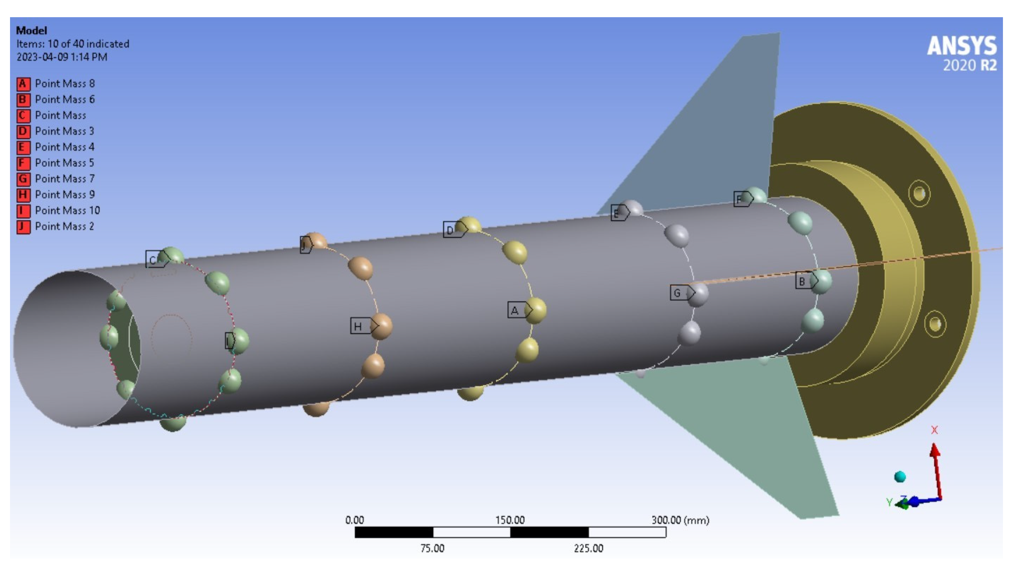
As this is a modal analysis, no load conditions were placed on the model. To acquire the actual deformation and stresses due to modal frequencies, a separate vibrational analysis would have to be conducted. However, when the material properties were assigned to the rocket assembly, the resulting mass was not inclusive of additional substances such as external paint or epoxy used to connect the components (Rocket Mass#0). To ensure the accuracy between the numerical and experimental model, 40 remote masses were evenly distributed over the aerostructure to account for these effects. This distribution can be seen in Figure 3.

Since the exact mass of these items was not provided, this value had to be estimated. Based on discussions with the team, an upper estimate of 3.3 kg and lower estimate of 2.5 kg was calculated. As will be reported and discussed in Section 4, both estimates were used in the numerical analysis and compared with experimental data (Rocket Mass#1 and Rocket Mass#2).

3.1.4. Boundary Conditions and Connections

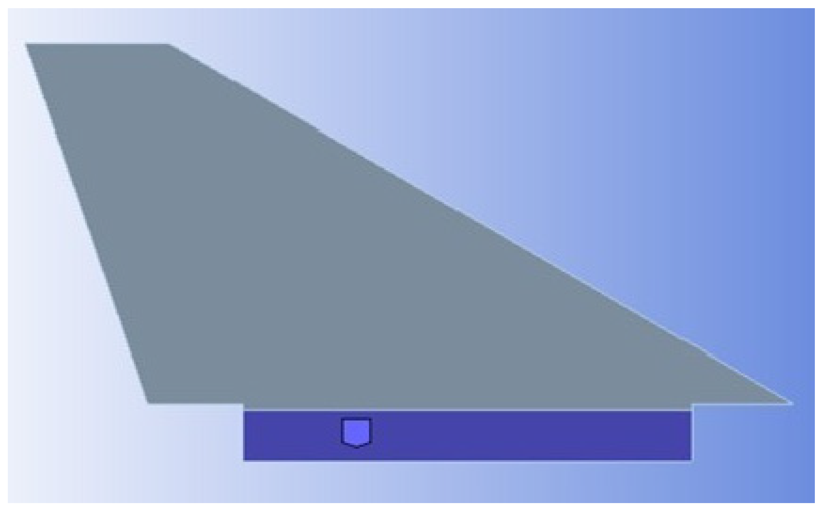
The isolated rocket fin was modeled as being clamped along the support table. The boundary conditions were kept simple. Additionally, a small gap of 1/16 in was placed between where the clamped condition was applied and where the tab ended. This was to ensure the fin did not slip or become misoriented during the actual experiment. The fin, with its fixed boundary condition, is shown in Figure 4.

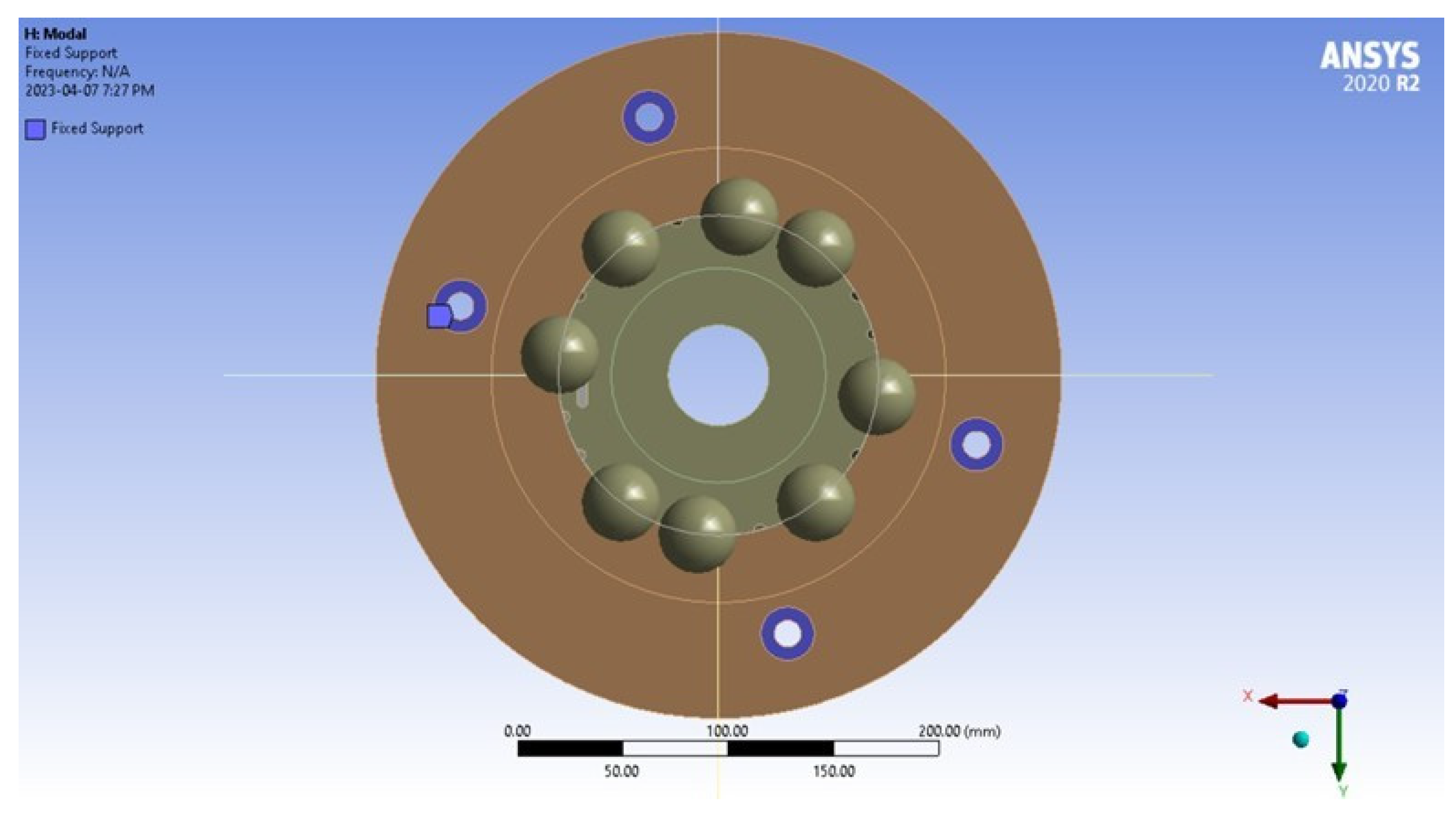
Within the modal workflow, all connections must be linear and therefore simplified down to bonded or no separation contacts. Since all the connections within the aerostructure are epoxied or friction fit, these were replaced with the bonded condition. As an example, the top and bottom surfaces of the boat tail coupler have bonded connections to the boat tail and the booster tube, respectively. The circular support structure was also bonded to the aerostructure, with its attachment holes then given a fixed condition. The boundary conditions of the rocket aerostructure are shown in Figure 5.

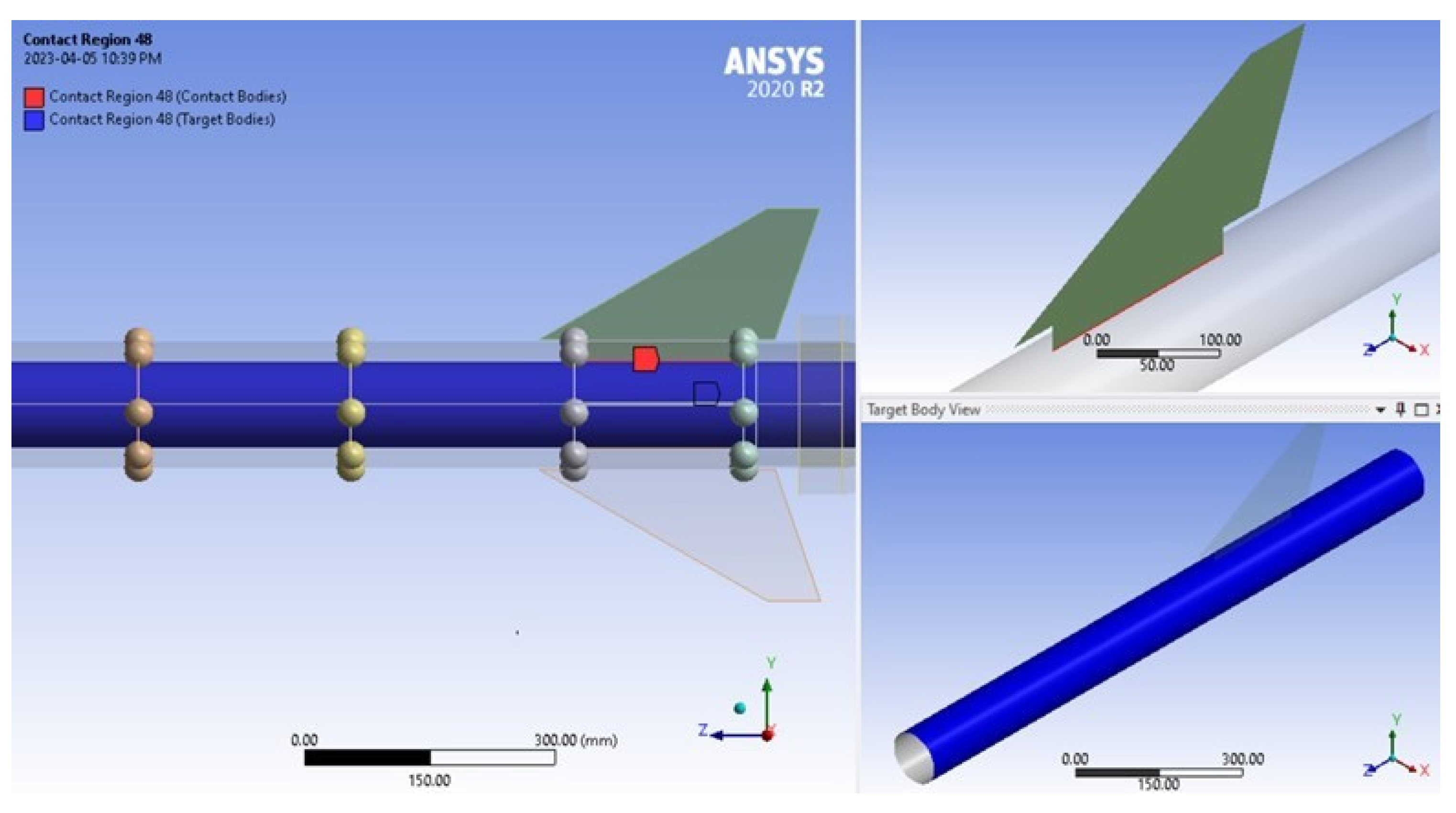
Since the attached rocket fin is a subcomponent of the rocket aerostructure, its analysis will be performed in the same model using the same connections. The fins are connected to the rest of the rocket aerostructure through a few connection points. The 1 in tab of the fin is placed inside the booster tube and the widths of the tab contact the first and second centering ring from the bottom of the motor tube. The longer side of the tab is placed firmly against the motor tube; these connections can be seen in Figure 6. At all these contacts points, the fins are epoxied using a mixture of aero-epoxy and strands of carbon fiber. These connections are represented in Ansys as bonded contacts.

3.1.5. Meshing

There were two meshes created for the isolated rocket fin and the complete rocket aerostructure. As mentioned above, the attached rocket fin utilized the same mesh as the rocket aerostructure since it was part of the model. The isolated rocket fin only consisted of one surface geometry, whereas the aerostructure model consisted of surfaces for the rocket and a solid body for the support. Although the mesh settings differed between the two, the surface meshes for both models were still generated using Shell181 elements. These elements feature 6 degrees of freedom (DOF) per node, with an element having 24 DOFs in total. The circular MDF support geometry was meshed using the default solid tetrahedral elements. The node and element count for each mesh are provided in

Table 3. Isolated Rocket Fin Mesh Statistics.

Mesh	Nodes	Elements
Super-Coarse	660	604
Coarse	1393	1310
Medium	2441	2334
Fine	5353	5190
Super-Fine	20,915	20,594

and

Table 4. Rocket Aerostructure Mesh Statistics.

Mesh	Nodes	Elements
Super-Coarse	58,217	44,138
Coarse	87,447	69,032
Medium	146,319	116,924
Fine	369,716	295,160

below. Although the complete rocket aerostructure mesh was meant to also reach super-fine mesh refinement, computational limits prevented this.

These mesh grades were also used to conduct a mesh independence study, which is further explained in Section 4.1.4. Figure 7 displays the refined mesh of the rocket aerostructure below.

3.2. Experimental Setup

This section details the three experimental setup configurations created. The first configuration was used to perform modal analysis for the isolated rocket fin, the second was for the rocket aerostructure, and the third was for the attached rocket fin. This section also details the equipment used for the modal analysis.

3.2.1. Equipment

The equipment was kept the same across all configurations of the experiment. The equipment itself can also be divided into two categories based on its use: vibrometry equipment and structural equipment. The main part of the vibrometry equipment is the MTI Instruments Microtrak III Laser Sensors. These sensors come with several advantages, as Laser Doppler Vibrometers (LDVs) can measure remotely and are not attached to the structure being measured. This means that there are no added mass effects or transverse sensitivities that need to be accounted for. Additionally, these instruments are highly accurate and can detect even the smallest movements, which is especially important since the composite rocket body is extremely rigid. Therefore, using laser vibrometers gives the best chance of measuring the modal frequencies with the least amount of calibration required. The vibrometry equipment also included the following [12,14]:

• Laser Sensor Interface (Duram Instruments).
• Data Amplifier Unit (HBM X400A).
• Power Supply Unit.
• Laptop PC.

The lasers are powered by 24V-DC outputted from the power supply unit. The lasers and the power supply unit are connected through the laser sensor interface, which also sends the collected analog signal to the data amplifier unit. The measurements are then sent to the PC where the HBM Catman AP software provides the results, such as displacement data and the frequency response function. The setup for the LDV is straightforward and can be represented by the diagram shown in Figure 8 [15].

The structural equipment consists of items such as aluminum extrusions, brackets, clamps, and the 3D-printed vibrometer holders. These items are all utilized to create the experimental support structures on which the laser sensors are mounted in the required locations depending on the component being tested. It is imperative that when creating the setup for the lasers, they must be placed at the correct standoff distance. According to the manufacturer’s specification, the LTS-050-10 lasers must be set up 50 mm ± 5 mm from the surface being measured.

3.2.2. Setup Configurations

Three setup configurations were created, each based on the component being tested. The first setup configuration that was created for the isolated rocket fin is shown in Figure 9 below. The fin was placed within two aluminum extrusions that were then clamped together on either side of the fin. This was undertaken to represent the fixed boundary condition from the numerical simulation. To ensure the extrusions could be adjusted, they were secured by clamping instead of using fasteners. The same strategy was used for the extrusions to the left of the fin, which served as the base for the laser vibrometers. The LDVs were attached to the aluminum extrusions using 3D-printed mounts that had been utilized for similar experiments previously.

The second configuration setup was created for the rocket aerostructure as shown in Figure 10. The rocket itself was placed within a pre-existing hole in the table. Since the hole diameter was smaller than the rocket diameter, an annular MDF support was designed and manufactured to keep the rocket rigid and leveled. The aluminum extrusions were reconfigured to create a setup that placed the lasers along the vertical axis of the rocket, with each of the sensors spaced about 1.25 ft apart. Additionally, to ensure the vibrations from the impact did not affect the measurements by the sensors, the entire vibrometer structure was placed on a separate table surface. This vibrometer support structure was also clamped to the table surface to allow for any adjustments required.

The third configuration utilized the exact same vibrometer support structure as the second configuration, with a few minor adjustments. First and foremost, since the rocket fin was being tested, there was minimal concern that the vibrations could transfer through multiple components and impact the sensor measurements. Therefore, the vibrometer support structure was placed on the table. Lasers 1 and 2 were also stacked close to one another, as shown in Figure 11, and provided the measurements for the experiment. Given that two sensors are more than sufficient for providing the measurements, laser 3 was not required.

4. Analysis

With all parameters and setup completed as presented in the previous sections, this section analyzes the data collected through both the numerical simulations and experiments. As implemented previously, this section will also be split into three separate subsections detailing the results for the isolated rocket fin, rocket aerostructure, and attached rocket fin, respectively. Additionally, for each of the simulation studies conducted, a mesh convergence study was completed to ensure that none of the discrepancies encountered were mesh related. More details concerning the study are provided in Section 4.1.4.

4.1. Numerical Observations

4.1.1. Isolated Rocket Fin

The isolated fin model was easily analyzed, as it was a single component with very simple boundary conditions. The numerical analysis was set to only calculate the first six modes for the fin, as provided in

Table 5. Isolated Rocket Fin Numerical Results.

Mode	Frequency (Hz)
1	84.05
2	307.70
3	412.74
4	679.96
5	1080.4
6	1109.2

.

The first mode shape is shown in Figure 12.

The first mode shape is also a purely bending mode, as the figure shows no twisting. As can be seen from Figure 12, the max deflection starts from the tip of the fin and continues inward on a diagonal path. This occurs as the areas closer to the tab or further down the fin are stiffer and therefore see less deflection.

4.1.2. Rocket Aerostructure

As mentioned previously, when the material properties were assigned to the rocket assembly, the resulting mass was not inclusive of additional materials such as the external paint or epoxy used to connect the components (Rocket Mass Model#0). Therefore, remote masses were distributed on the rocket to simulate extra weight due to paint and epoxy and to ensure the rocket was simulated as closely as possible to the experimental setup. The frequency results were calculated based on the original (Mass Model #0) and each mass estimate, with Mass Model #1 being 2.5 kg and Mass Model #2 being 3.3 kg. In addition, to account for the mass distribution, a layer of paint with a thickness of 1.875 mm was added as part of the composite layup. The only material properties specified for the paint were density, modulus of elasticity, and Poisson’s ratio [16]. Given that the stiffness of paint is negligible, most estimates put the young’s modulus at 1 GPa with a Poisson ratio of 0.2 (Mass Model #3). These results are shown in

Table 6. Rocket Aerostructure Numerical Results.

Frequency (Hz)
Mode	Mass Model #0	Mass Model #1	Mass Model #2	Mass Model #3
1	53.42	32.49	29.56	30.53
2	61.83	37.52	34.16	36.06
3	88.55	88.54	88.54	88.54
4	88.68	88.69	88.68	88.68
5	94.63	94.60	94.62	94.62
6	104.2	104.2	104.2	104.2

and provide the modal frequencies for both the main rocket body as well as the attached fins. The first two modal frequencies represent the bending modes for the main rocket aerostructure. Since the rocket is of a cylindrical cross section, one would expect that the two orthogonal bending modes should occur at the same frequency. However, there are discrepancies as the structure is quasi-orthotropic and not isotropic. Another source of discrepancy can be the positioning of the support attachment holes. As also discussed in Section 3.1.1, the holes were drilled at specific locations to ensure adequate spacing between them (the current holes in the steel table and the new ones). Due to this positioning, the rocket would have an easier time bending one way rather than the other. The rocket model was able to achieve mesh convergence on the fine mesh (see Table 3).

The first mode shape is shown in Figure 13.

4.1.3. Attached Rocket Fin

Due to the multielement nature of the rocket aerostructure, the numerical results for the fin were also collected to ensure the simulation’s accuracy. In Table 6, the modal frequencies for all four fins are displayed as the mode shapes three to six. Additionally, the first mode shape of the attached rocket fin is shown in Figure 14.

As also seen here, the mode shapes for all the fins are purely bending, with no twisting occurring. Parallel to the rocket mode shapes, the symmetrical nature of the rocket should mean that all fins experience the same modal frequency. It should be noted that this is true, as mode shapes 3 and 4, which represent fin groups (1 and 4) and (2 and 3) respectively, do vibrate at the same frequencies. However, the remaining two mode shapes, 5 and 6, could occur due to the orientation of the fins with respect o the support and the resulting change in their moment of inertia.

4.1.4. Mesh Convergence Study

As mentioned in Section 3.1.5, both models underwent mesh refinement to ensure the convergence of modal frequencies. Due to computational and resource limits, the isolated fin mesh was refined six times, whereas the complete rocket aerostructure mesh was only refined five times. All other details concerning the meshes are provided in Section 3.1.5. To conduct the mesh convergence study, the first modal frequency for each of the simulations was plotted against their respective element counts. The convergence results are provided in

Table 7. Isolated Rocket Fin Mesh Convergence.

Mesh	First Mode (Hz)	Elements	Rate of Change
Super-Course	84.62	604	-
Course	84.50	1310	1.76 × 10−4
Medium	84.35	2334	1.48 × 10−4
Fine	84.21	5190	4.76 × 10−5
Super-Fine	84.05	20,594	1.04 × 10−5

,

Table 8. Rocket Aerostructure Mesh Convergence.

Mesh	First Mode (Mass #1) (Hz)	Elements	Rate of Change
Super-Course	33.53	44,138	-
Course	33.19	69,032	1.39 × 10−5
Medium	32.90	116,924	5.99 × 10−6
Fine	32.49	295,160	2.29 × 10−6

and

Table 9. Attached Rocket Fin Mesh Convergence.

Mesh	First Mode (Hz)	Elements	Rate of Change
Super-Course	98.38	44,138	-
Course	96.87	69,032	6.07 × 10−5
Medium	95.77	116,924	2.31 × 10−5
Fine	94.01	295,160	9.84 × 10−6

for all three simulations.

As shown in Table 7, the isolated rocket fin numerical solution was able to converge to a final value of 84.05 Hz at the final mesh. In Table 7, the frequency rate of change between the meshes has also been provided. As seen in the table, although the rate of change decreases from one mesh to another, it is relatively negligible. This very same trend can be seen in the convergence datasets provided in Table 8 and Table 9. As the rate of change continues to decrease, the changes in the first mode frequency from mesh to mesh are negligible. Therefore, the rocket aerostructure numerical solution tested for Mass #1 converged to 32.49 Hz and the attached rocket fin solution converged to 94.01 Hz. The same mesh was then used for all the subsequent simulations.

4.2. Experimental Observations

4.2.1. Isolated Rocket Fin

The isolated rocket fin experiment was conducted first to validate the experiment process. Additionally, to ensure repeatability and a proper sample size, the experiment was conducted five times. The results from all five tests are included in

Table 10. Isolated Rocket Fin Experimental Results.

Test	Laser Sensor	Frequency (Hz)	Displacement (mm)
1	Laser 1 Laser 3	80.13 80.13	0.1574 0.03156
2	Laser 1 Laser 3	80.13 80.13	0.1586 0.03262
3	Laser 1 Laser 3	80.13 80.27	0.1251 0.03413
4	Laser 1 Laser 3	80.13 79.98	0.1327 0.02498
5	Laser 1 Laser 3	80.13 80.13	0.2060 0.04196

below.

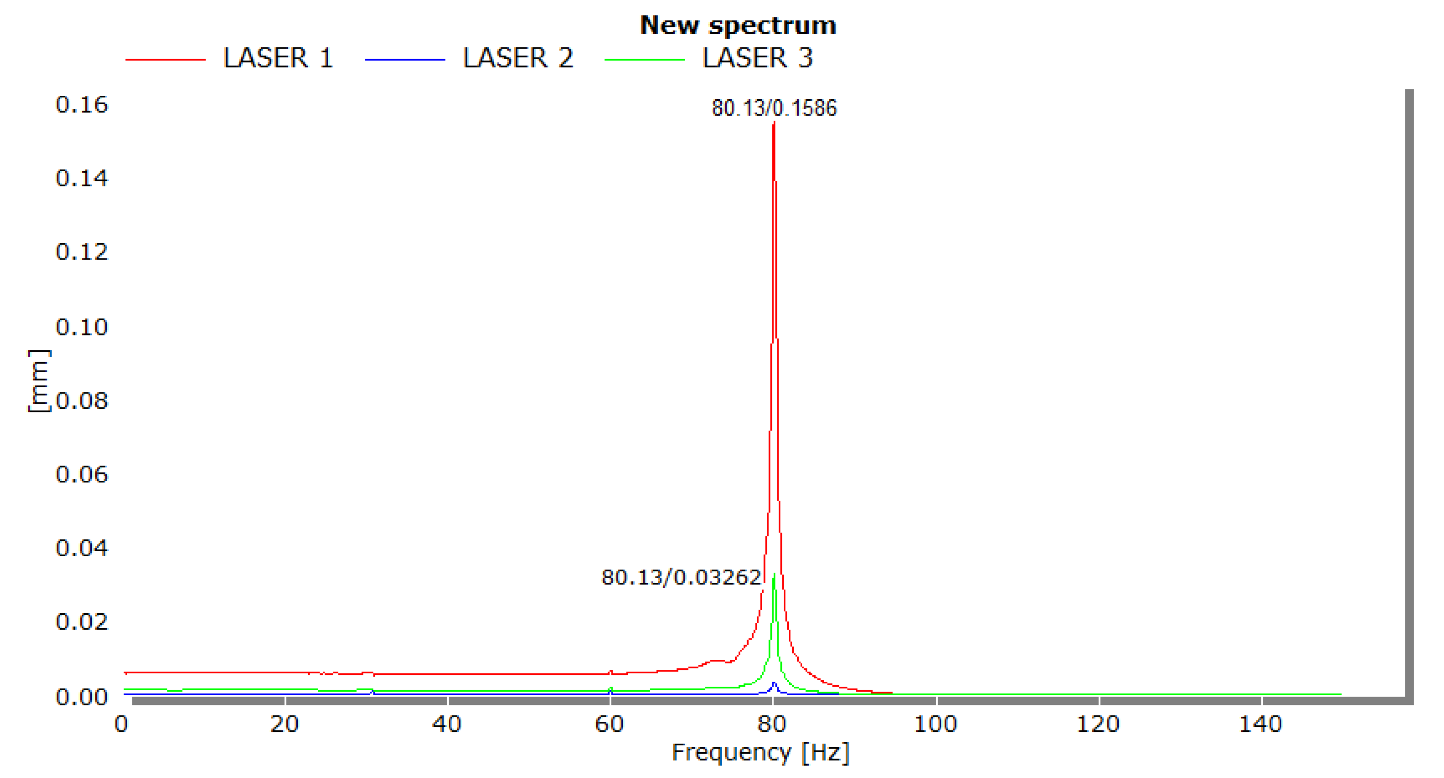
The resulting frequencies from the dataset were averaged to make 80.13 Hz, with a standard deviation of 0.07 Hz. The frequency response function from one of the trials is also provided below in Figure 15.

As seen from Figure 15, the response of the impulse excitation was extremely clean and a precise reading was collected across all three lasers. Additionally, all lasers showed agreement in terms of the modal frequency for all five trials. Unfortunately, due to the very small amplitude of laser 2 for most trials, the software was unable to pick up the displacements. However, a small peak can still be seen at the 80 Hz point from laser 2. All other frequency plots collected from this experiment have been provided in Appendix A.

4.2.2. Rocket Aerostructure

The setup for the rocket aerostructure’s experimental modal analysis was more complex. As shown in Section 3.2.2, the experiment involved constructing a structure with the sensors positioned along the central axis of the main rocket body. This allowed the first mode shape of the main rocket body to be recorded. Additionally, as mentioned above, the laser instrumentation equipment was placed on a separate table to ensure the measurements were isolated from the vibrations. The resulting modal frequencies collected from the FRF graphs are presented in

Table 11. Rocket Aerostructure Experimental Results.

Test	Laser Sensor	Frequency (Hz)	Displacement (mm)
1	Laser 1 Laser 2 Laser 3	27.25 27.25 27.25	0.00540 0.00774 0.01068
2	Laser 1 Laser 2 Laser 3	27.25 27.25 27.54	0.00494 0.00712 0.00983
3	Laser 1 Laser 2 Laser 3	27.54 27.54 27.54	0.00432 0.00623 0.00935
4	Laser 1 Laser 2 Laser 3	27.25 27.25 27.54	0.00507 0.00735 0.00994
5	Laser 1 Laser 2 Laser 3	26.95 26.95 27.25	0.00680 0.00998 0.01600

.

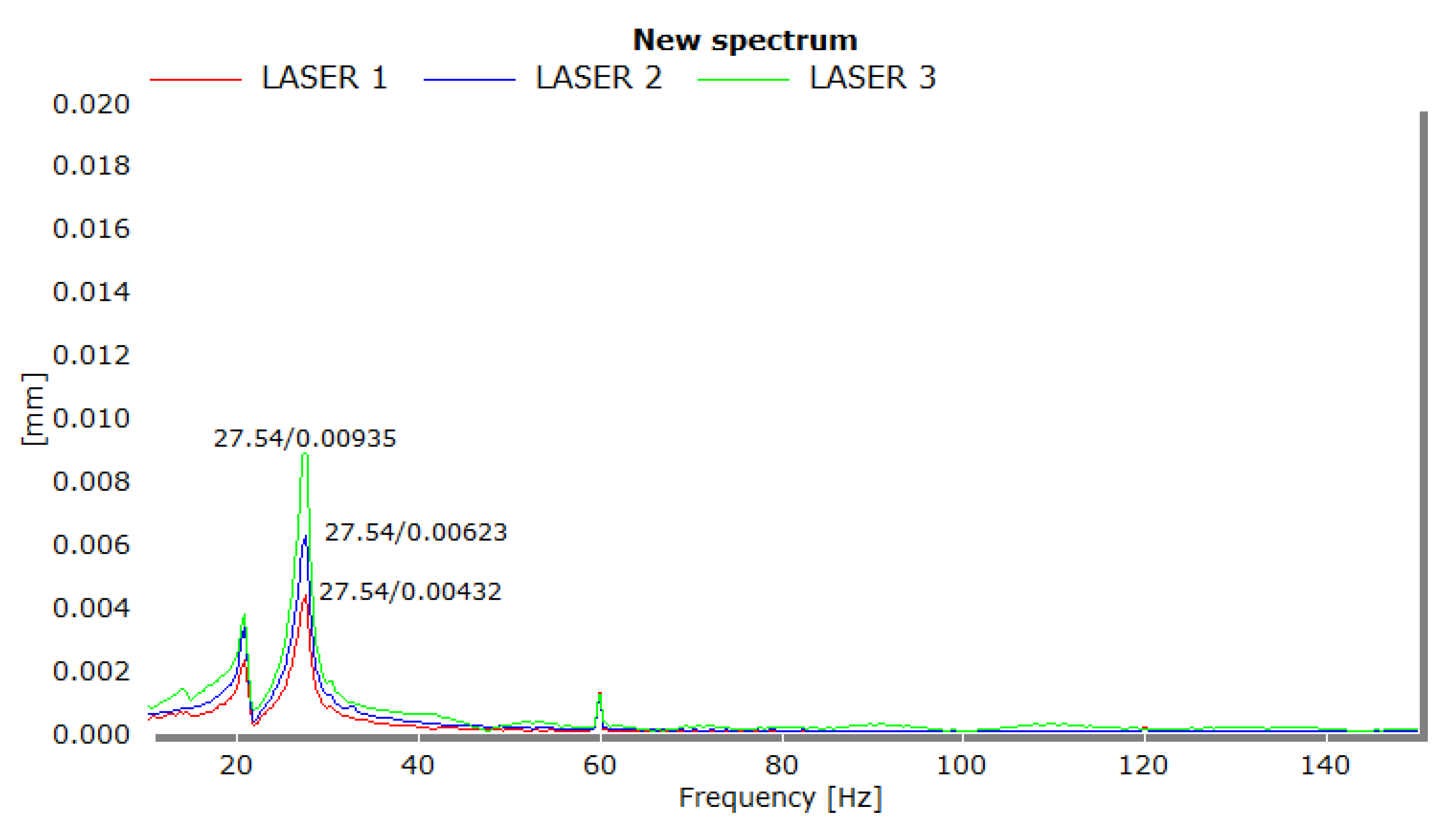
The modal frequency for the rocket aerostructure came out to an average of 27.3 Hz, with a standard deviation of 0.2 Hz. Due to the larger amplitude of displacements, as seen in Figure 16, all three lasers were able to record the same modal frequency. There are additional peaks in the FRF graph, such as at 60 Hz, that are associated with the electrical current frequency. There is another peak that occurs before the modal frequency of the rocket aerostructure at 20 Hz. Currently, it is unknown to the authors what the cause of this frequency might be. Considering that the rocket is a multielement structure, this peak could be associated with an internal component or its surrounding environment.

4.2.3. Attached Rocket Fin

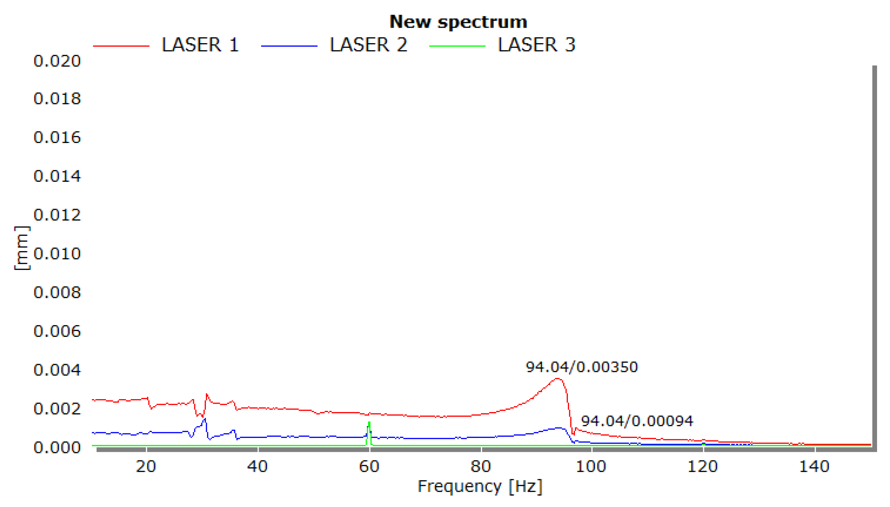
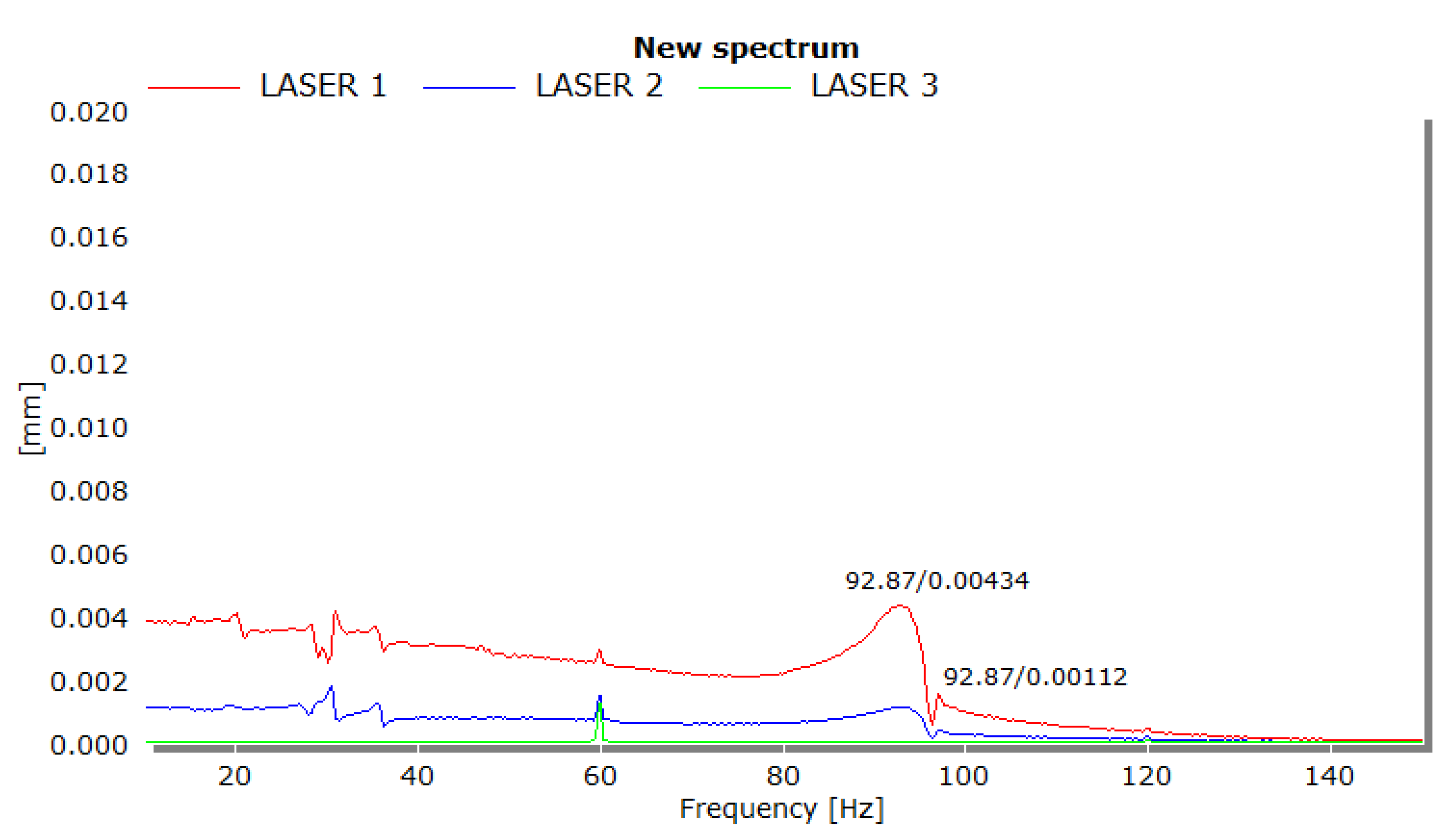
The final modal experiment conducted was the attached rocket fin, where given the reduced space for this setup, only two lasers (Laser 1 and 2) were utilized for data collection. However, since multiple lasers are only used as a redundancy, this was fine. The acquired data over five trials is presented in

Table 12. Attached Rocket Fin Experimental Results.

Test	Laser Sensor	Frequency (Hz)	Displacement (mm)
1	Laser 1 Laser 2	94.04 94.04	0.00350 0.00094
2	Laser 1 Laser 2	93.46 93.46	0.00401 0.00105
3	Laser 1 Laser 2	92.87 92.87	0.00434 0.00112
4	Laser 1 Laser 2	92.87 92.87	0.00338 0.00091
5	Laser 1 Laser 2	93.46 93.46	0.00353 0.00094

.

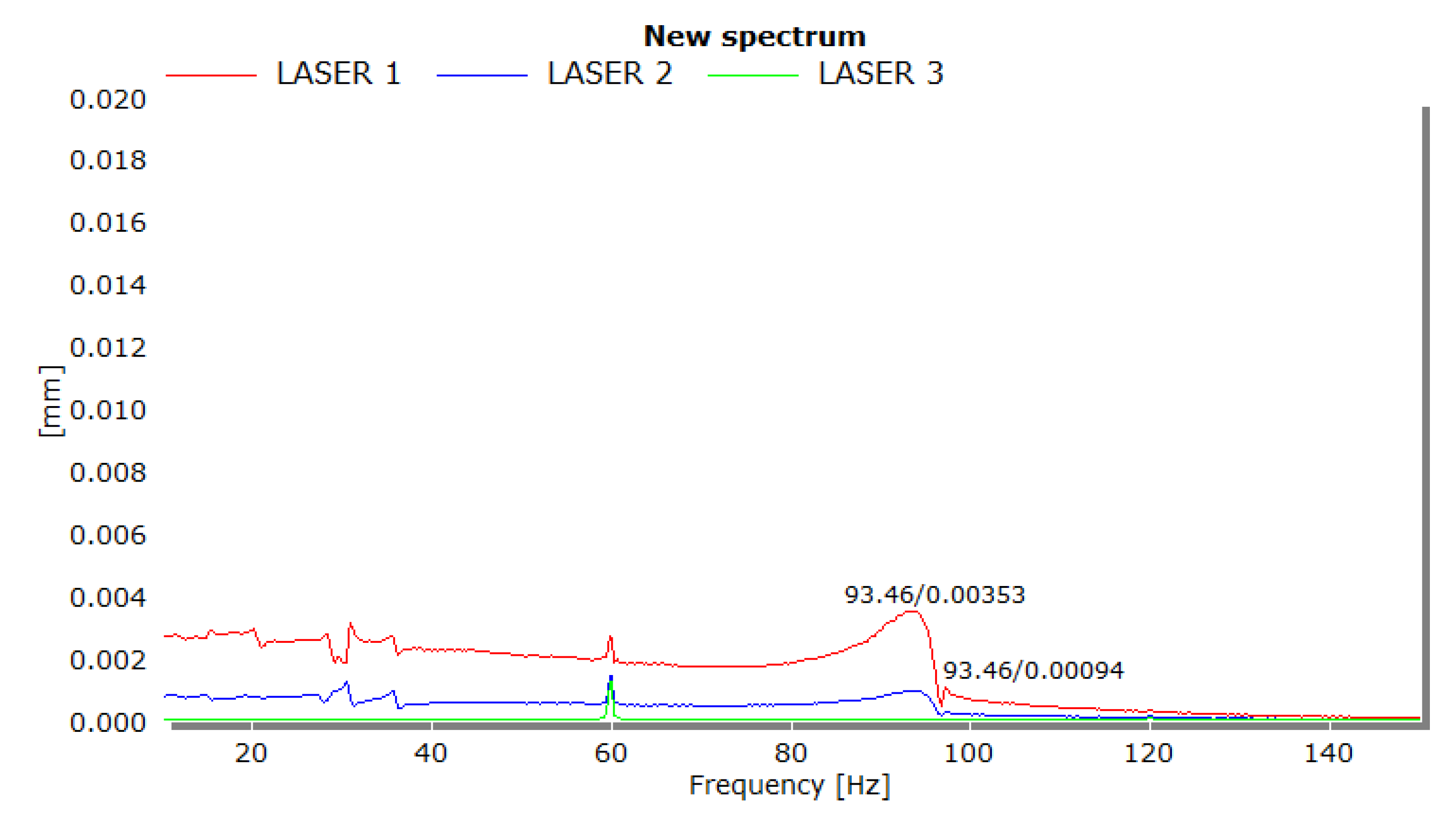
As can be seen from Table 12, the results are very consistent, with an average frequency of 93.34 Hz and a standard deviation of 0.41 Hz. Figure 17 provides the FRF graph for the experiment. As in the rocket experiment, the graph also features a spike at 60 Hz that is associated with electrical current frequency. However, unlike previous FRF graphs, the peaks of the modal frequency are less pronounced and more rounded, which could point towards higher dampening. This behavior is realistic as the fins have been inserted inside the rocket aerostructure with the connection points epoxied with a mixture of aero-epoxy and carbon fiber particulates.

5. Discussion

With the previous section having covered both the numerical and experimental data, this section will provide a comparison of the two. This section will also discuss the possible sources of discrepancies and perform a root cause analysis.

5.1. Data Comparison

Having verified the numerical data through a mesh convergence study and the experimental data through multiple trials, these datasets can now be compared against one another. Both datasets for all three components are summarized in

Table 13. Experimental and Numerical Data Comparison.

Test Article	Experimental (Hz)	Numerical (Hz)	Difference
Isolated Rocket Fin	80.13	84.05	4.89%
Original Rocket Model (Mass#0) 1st Refined Rocket (Mass#1)	27.31 27.31	53.42 32.49	95.6% 19.0%
2nd Refined Rocket (Mass#2) 3rd Refined Rocket (Mass #3)	27.31 27.31	29.56 30.53	8.24% 11.8%
Attached Rocket Fin	93.34	94.01	0.71

.

Generally, the experimental and numerical results for both the isolated and attached rocket fins are in good agreement with one another. The isolated rocket fin numerical result is within 5% of that obtained experimentally. The attached rocket fin was even closer, with a percent difference of less than 1% between the numerical and experimental results. The rocket aerostructure without any calibration has a percent dissimilarity of 96%; however, once the mass estimates are considered, this reduces to 19%, 8%, and 12% for mass estimates #1, #2, and #3, respectively. These differences can be explained by a few possibilities that are discussed in the next section.

5.2. Numerical and Experimental Errors

The sources of error for each of the test results will be discussed in the order of their appearance in Table 13, with the first being the isolated rocket fin. The isolated rocket fin only had a 5% difference between the experimental and numerical results, with the FEA modeling overestimating the modal frequency. This 5% difference can be explained by the fact that the FEA model would be stiffer than the actual experimental test article. Upon inspection of the fin, there is a shortage of carbon fiber, with only the epoxy remaining near the edges. Additionally, over the surface of the fin, there are areas where enough epoxy was not applied. Therefore, this discrepancy might be due to some manufacturing defects. In addition, it is worth mentioning that FEM models are, by nature, inherently stiffer than the real structure.

The rocket aerostructure is next and has the highest discrepancies compared with the other experiments. There are a few factors that could have contributed to this, namely, human error, support equipment, numerical simulation, and aerostructure defects. These factors have been summarized in the fish bone diagram shown in Figure 18.

The first two factors refer to the construction of the support attaching the rocket to the table. As also mentioned in Section 3.1.2, this support was manufactured using MDF material. Individual 1/8 in layers were assembled using wood glue to create the complete support geometry. Any remaining gaps between the inner diameter of the support and the outer diameter of the rocket body were then filled with plaster to ensure that the rocket was as rigid as possible. However, it could be that possible gaps between the layers or cracks within the plaster led to the support losing its rigidity. Additionally, during preliminary trials of the modal experiment, one of the layers of the MDF support delaminated due to the impact vibrations. Although this issue was resolved by applying epoxy to the area, there could be residual spaces left behind that could have reduced the support’s stiffness.

The third factor that could cause the discrepancy is pre-existing internal damage within the rocket. Although this rocket was visually inspected for damage before any testing began, there could be damage within the laminate layers that could lead to reduced stiffness and therefore a lower natural frequency. Finally, the fourth cause would be the structural complexity of the rocket itself. Within the booster tube, there are centering rings, bulkhead, motor tube, and fins. Each of these components are bonded to one another using epoxy. Additionally, as was mentioned in Section 3.1.3, the exact mass of the epoxy and paint were never recorded. Therefore, it is difficult to attribute an exact weight to the rocket, which could also be a source of the discrepancy. It should be noted that these are the remaining factors after the FEM model has already been calibrated.

The attached rocket fin is the final component that was tested. As mentioned above, the results were very similar, with only a 1% difference. Nonetheless, this discrepancy can be addressed by adding additional geometry to represent the bead of epoxy joining the fin to the rocket aerostructure, both internally and externally.

6. Conclusions and Future Work

In conclusion, the goal of this project was to conduct numerical and experimental modal analysis for a rocket aerostructure assembly and its sub-components. Ansys-based numerical simulations were first completed for all three test components. A composite model was created through Ansys ACP and then attached to a modal analysis workflow. All boundary conditions and connections were made to be as representative of the experimental setup as possible. There were some aspects of the test articles, such as damage to the rocket, that were not possible to model, as this information was either missing or could not be acquired. Nonetheless, this and other factors were accounted for by the authors as best as they could be with the information available, as well as other measurements. The comparison was then made between the numerical and experimental datasets; overall, the results were very close, with minor discrepancies. The isolated and attached rocket fin had very little percentage error between the experimental and numerical modal frequencies, with 5% and 1% differences, respectively. The original FEM model for the rocket aerostructure proved to be less accurate, with a percentage error of 96%; however, once the model was calibrated, this error fell to 19%, 8%, and 12% based on the mass estimates used. However, as discussed in Section 5.2, this discrepancy could be attributed to known sources of error. The series of experiments performed here have produced the resources and research framework that the Toronto Metropolitan Rocketry team can use to conduct further analyses on future rocket aerostructures and check their composite modeling setups. For future work, the current setups can be used to conduct the modal analysis of other components, sub-components, sub-assemblies, and the full rocket aerostructure, which includes the recovery sections and nosecone. This would help to further improve the current rocket model, which can then be used for other structural analyses.

References

- Chinta, V.S.; Reddy, P.R.; Prasad, K.E.; Raj, S.S. Modal Analysis of Carbon/Epoxy Plate By Varying Fibre Orientation. Adv. Mater. Res. 2021, 12, 7580–7586. [Google Scholar]
- Blom, A.W. Modal Test. In Structural Performance of Fiber-Placed, Variable-Stiffness Composite Conical and Cylindrical Shells; Wöhrmann Print Service: Zutphen, The Netherlands, 2010; pp. 121–130. [Google Scholar]
- Simsiriwong, J.; Sullivan, R.W. Vibration testing of a carbon composite fuselage. Int. J. Veh. Noise Vib. 2010, 6, 149. [Google Scholar] [CrossRef]
- Buehrle, R.D.; Fleming, G.A.; Pappa, R.S.; Grosveld, F.W. Finite element model development for aircraft fuselage structures. In Proceedings of the XVIII International Modal Analysis Conference, San Antonio, TX, USA, 7–10 February 2000. [Google Scholar]
- Cosco, F.; Serratore, G.; Gagliardi, F.; Filice, L.; Mundo, D. Experimental Characterization of the Torsional Damping in CFRP Disks by Impact Hammer Modal Testing. Polymers 2020, 12, 493. [Google Scholar] [CrossRef] [PubMed]
- Ansys, “Ansys Training,” Ansys Mechanical Linear and Nonlinear Dynamics. Available online: https://www.ansys.com/training-center/course-catalog/structures/ansys-mechanical-linear-and-nonlinear-dynamics (accessed on 18 April 2023).
- Barbero, E.J. Finite Element Analysis of Composite Materials Using Ansys; CRC Press: Boca Raton, FL, USA, 2014. [Google Scholar]
- Barbero, E.J. Introduction to Composite Materials Design; CRC/Taylor & Francis: Boca Raton, FL, USA, 2018. [Google Scholar]
- Stefano, R. A Twenty DOF Element for Nonlinear Analysis of Unsymmetrically Laminated Beams. Master’s Theses, Virginia Tech, Blacksburg, VA, USA, 1987. [Google Scholar]
- Maiti, D.K.; Sinha, P.K. Bending and free vibration analysis of shear deformable laminated composite beams by finite element method. Compos. Struct. 1994, 29, 421–431. [Google Scholar] [CrossRef]
- Li, J.; Hua, H.; Shen, R. Dynamic stiffness analysis for free vibrations of axially loaded laminated composite beams. Compos. Struct. 2008, 84, 87–98. [Google Scholar] [CrossRef]
- Piersol, A.G.; Paez, T.L.; Harris, C.M. Harris’ shock and Vibration Handbook; McGraw-Hill: New York, NY, USA, 2010. [Google Scholar]
- Chang, A.; Trivedi, S.; Jundi, M.; Qaumi, T.; Oyama, Y.; Ciniello, A.; Zain Aldeen, A.Z.; Mugisha, K.M. Development of Ryerson’s Fifth Spaceport America Cup Supersonic Rocket. Internal Report; Ryerson Rocketry Club, Presently MetRocketry: Toronto, ON, Canada, 2022. [Google Scholar]
- “Material Properties” Material Properties/Filament-Wound Composite Structures. Available online: https://www.amalgacomposites.com/material-properties.php (accessed on 1 November 2021).
- Khan, S. Design of an Out-Of-Autoclave Resin Transfer Molding Procedure for a Super-Sonic Rocket Fin. Bachelor’s Thesis, Department of Aerospace Engineering, Ryerson University, Toronto, ON, Canada, 2017. [Google Scholar]
- Freeman, A.A.; Fujisawa, N.; Bridarolli, A.; Bertolin, C.; Łukomski, M. Microscale Physical and Mechanical Analyses of Distemper Paint: A Case Study of Eidsborg Stave Church, Norway. Stud. Conserv. 2023, 68, 54–67. [Google Scholar] [CrossRef]
Figure 1.
Rocket Aerostructure Surface Model.
Figure 2.
Support Model; side view (left), and isometric view (right).
Figure 3.
Point Mass Distribution.
Figure 4.
Isolated Rocket Fin Boundary Condition.
Figure 5.
Rocket Aerostructure Fixed Boundary Condition.
Figure 6.
Attached Rocket Fin Connection with Motor Tube (left), the Fin’s tab insertion in the outer shell (top-right), and the Motor Tube (bottom-right).
Figure 7.
Complete Rocket Aerostructure Mesh.
Figure 8.
Laser Vibrometry Setup.
Figure 9.
Experiment Configuration #1.
Figure 10.
Experiment Configuration #2.
Figure 11.
Experiment Configuration #3.
Figure 12.
Isolated Rocket Fin First Mode Shape.
Figure 13.
First Mode Shape Rocket Aerostructure.
Figure 14.
First Mode Shape of Attached Rocket Fin.
Figure 15.
Isolated Rocket Fin Trial 1 Experimental FRF.
Figure 16.
Rocket Aerostructure Trial 1 Experimental FRF.
Figure 17.
Attached Rocket Fin Trial 1 Experimental FRF.
Figure 18.
Fishbone Diagram.