A Reduced Order Model for Monitoring Aeroengines Condition in Real Time

Abstract

A very fast reduced order model is developed to monitor aeroengines condition (defining their degradation from a baseline state) in real time, by using synthetic data collected in specific sensors. This reduced model is constructed by applying higher-order singular value decomposition plus interpolation to appropriate data, organized in tensor form. Such data are obtained by means of an engine model that takes the engine physics into account. Thus, the method synergically combines the advantages of data-driven (fast online operation) and model-based (the engine physics is accounted for) condition monitoring methods. Using this reduced order model as surrogate of the engine model, two gradient-like condition monitoring tools are constructed. The first tool is extremely fast and able to precisely compute the turbine inlet temperature ‘on the fly’, which is a paramount parameter for the engine performance, operation, and maintenance, and can only be roughly estimated by the engine instrumentation in civil aviation. The second tool is not as fast (but still reasonably inexpensive) and precisely computes both the engine degradation and the turbine inlet temperature at which sensors data have been acquired. These tools are robust in connection with random noise added to the sensor data and can be straightforwardly applied to other mechanical systems.

1. Introduction

The health condition of a mechanical system determines its performance. Thus, monitoring such condition is essential for various tasks, including control, maintenance, and safety. In particular, predictive maintenance (also called condition-based maintenance) requires monitoring the system condition for diagnosis [1,2,3,4] to anticipate when it should be repaired/restored before potentially dangerous breakdown occurs. Thus, predictive maintenance (i) reduces cost [5] because maintenance tasks are carried out when and where they are truly needed, not just by schedule, and (ii) increases safety by avoiding dangerous events during operation. This type of maintenance has received increased attention in the literature during the last decades [6,7,8], due to its application in a variety of industrial sectors, such as the aerospace [9,10], manufacturing [11], and railway [12] industries.

Although the methods developed in the paper apply to more general systems, they will be illustrated (and their performance tested) considering a turbofan aeroengine for commercial aviation. This system is representative, in terms of both difficulties and opportunities, of many other complex mechanical systems. The performance of the developed methodology will be tested for synthetic data in cruise conditions, which cover most part of the flight time. Similar results could be obtained considering other flight stages, such as take off and landing.

Concentrating on aeroengines, during the last decade, an increasing interest has arisen in the main industrial companies in the field on developing health monitoring tools to improve their predictive maintenance capability. Many of these tools are either data-driven or model-based [13,14]; additionally, there are hybrid methods, such as the physics-informed neural networks [15].

Purely data-driven methods [16] rely on just data and are usually based on machine learning and statistical algorithms. Their online operation is fairly inexpensive, but constructing these models requires offline training [17], the computational cost of which is usually enormous. It is performed using former experience in the type of engine that is being analyzed. They lack flexibility, since they do not give good results for other engines (or modified engines) not accounted for in the training stage.

Model-based methods are more flexible and precise than data-driven models because they explicitly take the aeroengine physics into account, using a nonlinear engine model. Thus, these methods require solving (iteratively) a large set of nonlinear equations, meaning that their online operation is generally more computationally expensive than that of data-driven models. The engine model computes the sensors outputs in terms of several degradation parameters that depend on the engine condition (health status) and the operating regime. The operating regime is determined by the flight altitude and Mach number, and the turbine inlet temperature. The latter is very important since it determines the engine thrust (and affects the engine lifetime) in aircraft aeroengines, as well as the engine power in related systems, such as naval gas turbines and aeroderivatives. Concerning the aeroengine degradation parameters, Stamatis et al. [18] proposed flow capacities and adiabatic efficiencies of several engine components, which are generally acepted nowadays. The main turbofan manufactures have developed their own models for the engines they produce. Unfortunately, these engine models are confidential and not available in the literature. In this paper, we shall use an engine model based on PROOSIS [19], which is able to simulate different aeroengine types; see [20] for details of the PROOSIS solver. It must be noted that this (and any other) engine model uses discrete empirical data obtained by actual measurements in the main engine components, and is based on an iterative method. The latter exhibits convergence difficulties when trying to simulate cases that are outside the operating regime where the empirical data have been acquired. A review of model-based methods can be found in our recent work [20], where a methodology was developed for aeroengine diagnosis. The present paper is a step further in the sense that, while diagnosis was performed in [20] using a PROOSIS-based engine model, here, we shall construct and use a convenient reduced order model (ROM), combined with gradient-like condition monitoring tools. In contrast with the engine model, the online operation of this ROM is extremely fast since it only requires to perform a limited set of algebraic computations. This means that the methodology to be developed in this paper shares the advantages of the data-driven and model-based methods, namely fast online operation and precise, robust results. In fact, we shall use the experience gained in [20] to directly select the most convenient gradient-like method, which is an appropriately adapted global, constrained Newton-based method that gives very good diagnosis results. Full details of this method, omitted here for the sake of brevity, can be found in [20]. The offline construction of the ROM requires: (i) running a full engine model a very large number of times, to obtain data that are collected in a (high-order) tensor; this may be fairly computationally expensive. Furthermore, (ii) applying a tensor decomposition, which instead is fairly inexpensive. As anticipated, the online operation of the ROM is quite fast, permitting real-time results. The concept of ’real time’ is somewhat ambiguous, since it has several possible meanings, depending of the context. To be precise, two meanings are used in this paper: (a) on the one hand, monitoring data in the aircraft cockpit requires a very small computational time, not larger than, say, 0.5 CPU seconds, which is enough for human eye detection and will be called continuous real time; (b) on the other hand, since the flight time is at least 30 min, a computational time of up to a few CPU minutes will be called in-flight real time.

Specifically, the ROM will be constructed by applying a tensor extension of standard singular value decomposition (SVD), called higher-order singular value decomposition (HOSVD), combined with one-dimensional interpolation, to a dataset organized in tensor form. This combination is a higher-dimensional extension of the celebrated, very useful method [21,22], which combines proper orthogonal decomposition (or standard SVD) and interpolation. The required data will be obtained using an engine model. In other words, a surrogate of the engine model will be constructed that gives the sensors outcomes in terms of the engine operating regime and the degradation parameters. Similar ROMs based on HOSVD plus interpolation have been already used in several fields, including generation of aerodynamic databases [23], continuous real-time control of reciprocating engines [24], and aircraft conceptual design [25,26]. HOSVD-based methods also permit constructing tools for recovering lost data [27] and filtering large errors [28] in multidimensional databases, which are relevant in condition monitoring tasks, including:

• Recovering sensors data not provided by the engine model, due to convergence difficulties. Furthermore, recovering data at places in the engine not accessible to sensor measurements.
• Correcting wrong sensors data due to ill-functioning sensors or engine instrumentation, which may produce large errors.

However, these applications are beyond the scope of this paper and will be considered elsewhere. Here, we shall only consider small errors in the sensors data that somewhat mimic experimental noise, see below.

Using the surrogate engine model, two condition monitoring tools will be developed that compute both the engine degradations and the turbine inlet temperature, $T_{4t}$, at which the sensors data have been acquired:

• The condition monitoring tool 1 is based on a linear approximation, and thus requires small degradations around a baseline state, which are expected in each individual flight. Its online operation is extremely fast; namely, it can operate in continuous real time. It precisely computes the turbine inlet temperature $T_{4t}$ and gives a first approximation of the engine degradation. This tool has been obtained as an unexpected byproduct, when checking the importance of nonlinear effects.
• The condition monitoring tool 2 is the counterpart, using the ROM surrogate, of a very efficient tool developed in [20] for the full engine model. This tool operates in in-flight real time and is designed for nonsmall degradations (up to ∼2%), for which nonlinear effects must be accounted for. Let us mention here that degradations of 2% are fairly high and usually require performing maintenance tasks on the degraded engine component [29,30,31] to avoid future dangerous events. On the other hand, the very small degradations that are expected during each flight accumulate in subsequent flights. In this sense, if an accumulated degradation becomes larger than 2%, then it must be monitored since it could reach dangerous values as time proceeds. Such monitoring can be performed using the method developed in [20], which accurately performs diagnosis for very large degradations. In this sense, the tool 2 developed in this paper is complementary to the methodology presented in [20].

The raw (dimensional) sensors data account for properties such as temperatures, pressures, rotational speeds, and fuel consumption, which take very disparate values. This could cause ill-functioning of condition monitoring tools. Thus, the sensors outcomes need to be appropriately nondimensionalized/scaled.

On the other hand, in practice, the outcomes of actual sensors mounted in the engine are noisy. In order to take this into account, small random noise with zero mean will be added to the engine model outcomes, concluding that the developed tools are robust in connection with noise.

Computations will be performed using standard (uncompiled) MATLAB in a standard PC, with a microprocessor Intel Core I7-6500U at 2.5 GHz, with 16 GB of RAM memory. The CPU times reported along the paper for reference could be significantly reduced using more advanced, customized software and hardware. Quantitative results will be given in the form of tables, which is convenient to facilitate the reader to reproduce results.

Against the above background, the remainder of the paper is organized as follows. The specific aeroengine that will be used to test the performance of the methodology is presented in Section 2, where the convenient degradation parameters and sensors are described and the output sensors data are appropriately scaled. The required data processing methods, standard SVD and HOSVD, are briefly described in Section 3, where the detailed construction of the surrogate engine model and the aforementioned condition monitoring tools 1 and 2 are also addressed. Specific condition monitoring results are given in Section 4 and some concluding remarks are provided in Section 5.

2. Test Case to Evaluate the Performance of the Methodology: The CFM56 Aeroengine

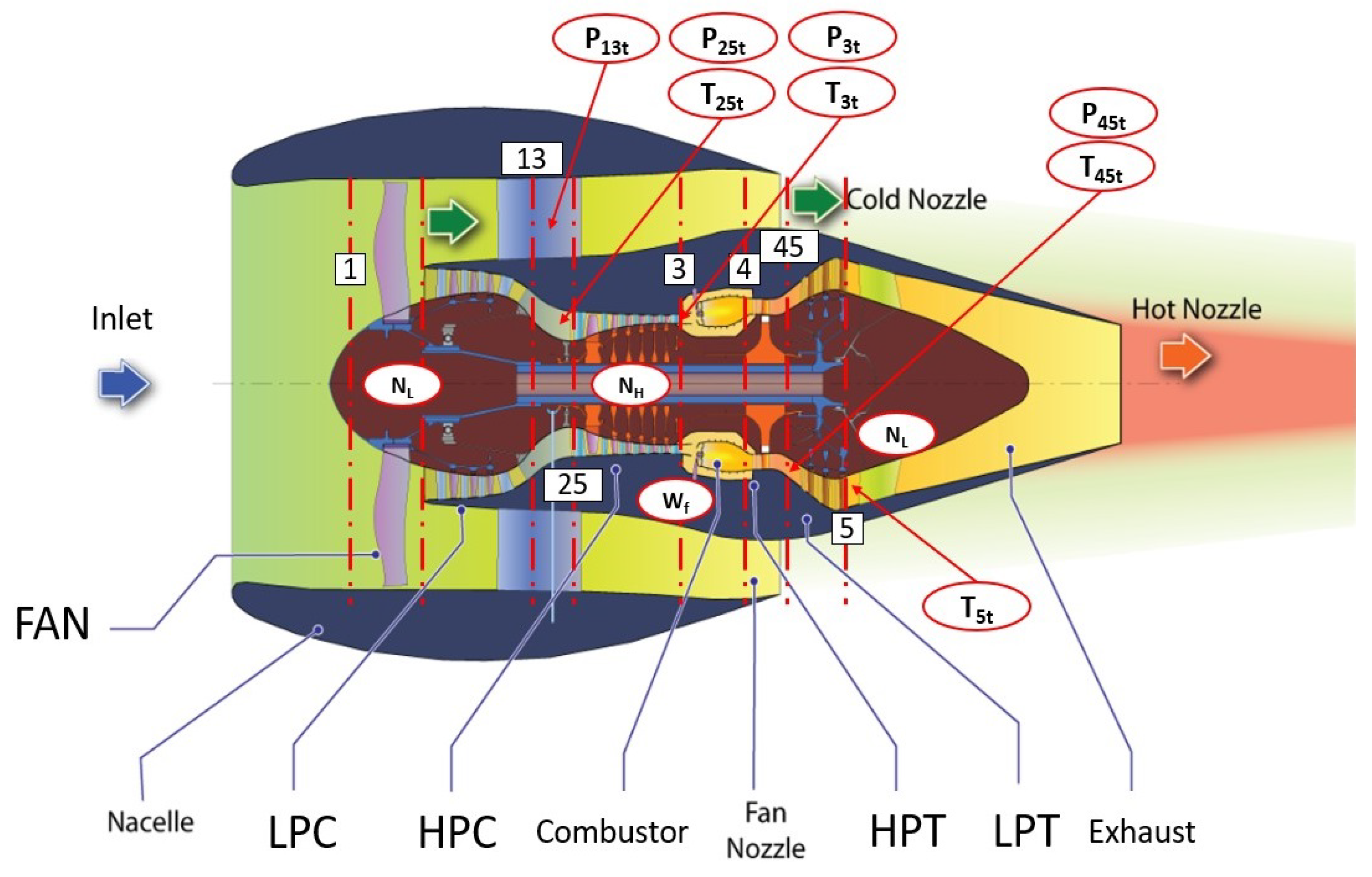
As in [20], we consider a CFM56 aeroengine, which is representative of those widely used in commercial aviation nowadays [32]. It is the two-spool turbofan engine sketched in Figure 1, where the main engine components are indicated, as well as the engine locations where several relevant pressures P, temperatures T, rotational speeds, $N_L$ and $N_H$, and the fuel consumption $W_f$ can be measured. As can be seen, the engine contains both a low-pressure spool and a high-pressure spool, which rotate concentrically at different speeds. The high-pressure compressor (HPC), the high-pressure turbine (HPT), and the combustor constitute the high-pressure part of the engine, also known as the core of the engine. The fan, the low-pressure compressor (LPC), also known as the booster, and the low-pressure turbine (LPT) are mechanically connected and constitute the low-pressure part of the engine. For the various involved technical parameters, see the Appendix in our previous work [33].

For this engine, condition monitoring will be performed in the following ranges of the flight altitude h, the Mach number M, and the turbine inlet temperature $T_{4t}$:

$$31,000\mathrm{ft}\le h\le 39,000\mathrm{ft},0.8\le M\le 0.86,1350\mathrm{K}\le T_{4t}\le 1550\mathrm{K},$$

(1)

which cover typical cruise conditions in commercial aviation.

The engine is characterized by the ten degradation parameters, whose deviation from their baseline values measure the engine degradation. They are measured in %, which represents an automatic scaling, and are nonnegative because the engine is degraded, not upgraded. In the present paper, as anticipated, they are allowed to vary in the following range:

$$0\le x_j\le 2,\mathrm{for}j=1\dots ,10.$$

(2)

The ten degradation parameters give the efficiencies and adiabatic capacities of various engine stations, as displayed in

Table 1. Description of the 10 degradation parameters for the CFM56 aeroengine sketched in Figure 1.

Degradation #	Degradation Description
1	$x_1={\eta }_{FAN}$: FAN efficiency
2	$x_2={\mathrm{\Gamma }}_{FAN}$: FAN flow capacity
3	$x_3={\eta }_{LPC}$: LPC efficiency
4	$x_4={\mathrm{\Gamma }}_{LPC}$: LPC flow capacity
5	$x_5={\eta }_{HPC}$: HPC efficiency
6	$x_6={\mathrm{\Gamma }}_{HPC}$: HPC flow capacity
7	$x_7={\eta }_{HPT}$: HPT efficiency
8	$x_8={\mathrm{\Gamma }}_{HPT}$: HPT flow capacity
9	$x_9={\eta }_{LPT}$: LPT efficiency
10	$x_{10}={\mathrm{\Gamma }}_{LPT}$: LPT flow capacity

.

Our condition monitoring tools will use sensors data to compute the ten degradations and the turbine inlet temperature, which amount to eleven unknowns. After the analysis in [20], we shall consider the eleven sensors described in

Table 2. Sensors description, and average values and standard deviations, of the sensor outcomes for the 11 sensors used for condition monitoring the CFM56 aeroengine. See Figure 1 for the engine locations of these sensors.

Sensor #	Description	Average Value	Standard Deviation
1	$y_1^{dimens.}=P_{13t}$	≃$6.0946·{10}^4$ Pa	0.15
2	$y_2^{dimens.}=P_{25t}$	≃$2.0068·{10}^5$ Pa	0.15
3	$y_3^{dimens.}=P_{3t}$	≃$1.3464·{10}^6$ Pa	0.15
4	$y_4^{dimens.}=P_{45t}$	≃$4.0060·{10}^5$ Pa	0.15
5	$y_5^{dimens.}=T_{25t}$	≃433.46 K	0.025
6	$y_6^{dimens.}=T_{3t}$	≃774.20 K	0.034
7	$y_7^{dimens.}=T_{45t}$	≃$1.0900·{10}^3$ K	0.050
8	$y_8^{dimens.}=T_{5t}$	≃729.00 K	0.054
9	$y_9^{dimens.}=N_L$	≃$4.0834·{10}^3$ rpm	0.035
10	$y_{10}^{dimens.}=N_H$	≃$1.0201·{10}^4$ rpm	0.029
11	$y_{11}^{dimens.}=W_f$	≃1.0427 kg/s	0.18

, second column, which are conveniently uncorrelated. In fact, the ten sensors 1–3 and 5–11 displayed in the table are representative of those frequently used in diagnosis studies [3,33,35,36,37], and are usually mounted in the CFM56 aeroengine instrumentation [38]. Concerning the 4th sensor, giving $P_{45t}$ (also included in the CFM56 instrumentation), this was selected in [20] as one that complements very well the remaining ten sensors.

The average values of the sensors and the associated standard deviations, displayed in the third and fourth columns of the table, have been computed from the outcomes using the full engine model at the 45 combinations of the following three values of the altitude h, three values Mach number M, and five values of the turbine inlet temperature $T_{4t}$:

$$\begin{array}{cc}& h=31,000,35,000,\mathrm{and}39,000\mathrm{ft},\hfill \end{array}$$

(3)

$$\begin{array}{cc}& M=0.8,0.83,\mathrm{and}0.86,\hfill \end{array}$$

(4)

$$\begin{array}{cc}& T_{4t}=1350,1400,1450,1500,\mathrm{and}1550.\hfill \end{array}$$

(5)

Note that these 45 combinations cover well the range defined in (1) in which the engine is to be inspected, and are necessarily computed because they will be precisely the discrete values of these parameters to construct the ROM. As can be seen in Table 2, the dimensional values of the sensors outcomes differ among each other by several orders of magnitude; moreover, the standard deviations are dissimilar, since there is a factor of ∼7 between the smallest and the largest. Thus, it is convenient to scale them in such a way that the scaled values are comparable and vary in comparable ranges. As thoroughly explained in [20], a convenient scaling meeting these requirements is performed as follows. The $N_{sensors}$ (=11 in the present case) scaled sensor outcomes, denoted as $y_1^{scal.},\dots ,y_{N_{sensors}}^{scal.}$, are calculated as follows:

$$y_m^{scal.}=\frac{y_m^{dimens.}-y_m^{aver.}}{sd\left(m\right)·y_m^{aver.}},$$

(6)

where, for $m=1,\dots ,N_{sensors}$, $y_m^{dimens.}$ are the original dimensional sensor outcomes, while $y_m^{aver.}$ and $sd\left(m\right)$ are the associated averages and standard deviations displayed in Table 2. Sensors will always be scaled using (6) in the paper. This scaling can be computed for any aeroengine, with any value of $N_{sensors}$ and, mutatis mutandis, to the sensor outcomes in other mechanical systems.

3. Methods and Tools

After briefly describing the well known SVD and HOSVD data processing tools, the construction of the surrogate model and the development of the already mentioned health monitoring tools 1 and 2 will be addressed.

3.1. Standard SVD and HOSVD

Standard SVD was introduced [39] by Beltrami and Jordan (in 1873–1874) for square matrices, and further developed by Eckart and Young [40] for general, rectangular matrices. There are many versions of SVD [41]. In the present version, for a real, generally rectangular, $I\times J$ matrix $\mathbf{A}$, its SVD is given by:

$$\mathbf{A}=\mathbf{U}\mathbf{S}{\mathbf{V}}^{\top }\mathrm{or}{A}_{ij}=\sum _{q=1}^Q{s}_q{U}_{iq}{V}_{jq},$$

(7)

where the superscript ${}^{\top }$ denotes the transpose and $\mathbf{U}$ and $\mathbf{V}$ are $I\times Q$ and $J\times Q$ matrices, respectively, with $Q=min\{I,J\}$; the columns of these matrices are mutually orthonormal with the usual Euclidean inner product. The matrix $\mathbf{S}$ is diagonal and its elements, known as the singular values and denoted as $s_n$, are real, nonnegative, and sorted in decreasing order, namely $s_1\ge s_2\ge \dots \ge s_Q\ge 0$. The decomposition (7) can be calculated using the MATLAB command ‘svd’, option ‘economy’. SVD is also useful to define the condition number of the matrix $\mathbf{A}$, which is directly computed with the MATLAB command ‘cond’. It indicates the accuracy when solving linear systems whose coefficient matrix is $\mathbf{A}$; such accuracy worsens as the condition number increases [42].

The extension of SVD to higher than two-order tensors (i.e., multi-dimensional databases) is highly nontrivial. There are many such extensions [43]. The most obvious one, known as the canonical decomposition, consists in reorganizing the tensor as a linear combination of rank-one tensors. The minimum number of rank-one tensors such that this decomposition is possible defines the rank of the tensor, whose computation for general tensors is an open problem still nowadays [44]. Because of this difficulty, other extensions have been developed. A very robust extension was introduced by Tucker [45] and more recently popularized by de Lathauwer et al. [46,47]. This extension, called higher-order singular value decomposition (HOSVD), is also known as the Tucker decomposition. For an N-th order tensor $\mathbf{T}$ of size $I_1\times I_2\times \dots \times I_N$, its HOSVD rewrites the tensor components as:

$$T_{i_1{i}_2\dots i_N}=\sum _{i_1^{\prime }=1}^{I_1}\sum _{i_2^{\prime }=1}^{I_2}\cdots \sum _{i_N^{\prime }=1}^{I_N}{S}_{i_1^{\prime }{i}_2^{\prime }\dots i_N^{\prime }}{U}_{i_1{i}_1^{\prime }}^1{U}_{i_2{i}_2^{\prime }}^2\cdots U_{i_N{i}_N^{\prime }}^N,$$

(8)

for $i_1=1,2,\dots ,I_1$, $i_2=1,2,\dots ,I_2$, …, $i_n=1,2,\dots ,I_N$. $S_{i_1^{\prime }{i}_2^{\prime }\dots i_N^{\prime }}$ are the components of an N-th order tensor $\mathbf{S}$, of size $I_1\times I_2\times \dots \times I_N$, and the square matrices ${\mathbf{U}}^1,{\mathbf{U}}^2,\dots ,{\mathbf{U}}^N$, of sizes $I_1,I_2,\dots I_N$, whose elements are $U_{i_1{n}_1}^1$, $U_{i_2{n}_2}^2\dots$, $U_{i_N{n}_N}^N$, are known as the mode matrices along the various dimensions of the tensor $\mathbf{T}$. Now, we note that the expansion appearing in (8) is a multilinear function of the components of the tensor $\mathbf{S}$ and the mode matrices, which can be considered as a tensor product of these. Thus, Equation (8) is rewritten as:

$$\mathbf{T}=\mathbf{tprod}(\mathbf{S},{\mathbf{U}}^1,{\mathbf{U}}^2,\dots ,{\mathbf{U}}^N).$$

(9)

A MATLAB function to compute this tensor product can be found in [48].

Let us now explain briefly how HOSVD is constructed. To begin with, for each $n=1\dots ,N$, the tensor $\mathbf{T}$ is unfolded (which can be done using a MATLAB function given in [48]) into the matrix ${\mathbf{A}}^n$, whose columns are the fibers of $\mathbf{T}$ along the n-th tensor dimension. Then, SVD is applied to the matrix ${\mathbf{A}}^n$, which gives:

$${\mathbf{A}}^n={\mathbf{U}}^n{\mathbf{S}}^n{\left({\mathbf{V}}^n\right)}^{\top }.$$

(10)

where the matrix ${\mathbf{U}}^n$ is precisely the mode matrix along the n-th dimension appearing in (9). Then, the tensor $\mathbf{S}$ is computed as:

$$\mathbf{S}=\mathbf{tprod}(\mathbf{T},{\left({\mathbf{U}}^1\right)}^{\top },{\left({\mathbf{U}}^2\right)}^{\top },\dots ,{\left({\mathbf{U}}^N\right)}^{\top }).$$

(11)

With this, all ingredients appearing in the right hand side of (8) have been calculated.

3.2. Construction of the HOSVD-Based Surrogate Engine Model

To begin with, we construct the following fourteenth-order tensor:

$$T_{i{j}_1{j}_2{j}_3{k}_1\dots k_{10}},$$

(12)

containing the (scaled as explained in Section 2) synthetic sensors data, obtained using the engine model, for the 45 combinations of the parameters defining the flight regime displayed in (3)–(5). In this tensor:

• For $i=1,\dots ,11$, the first index indicates the eleven sensors.
• For $j_1=1,2,3$, the second index corresponds to the three flight altitudes displayed in (3).
• For $j_2=1,2,3$, the third index is associated with the three Mach numbers appearing in (4).
• For $j_3=1,\dots ,5$, the fourth index indicates the five values of the turbine inlet temperature displayed in (5).
• The remaining ten indexes, $k_1,\dots ,k_{10}$, correspond to the ten degradations denoted as x and are allowed to take the following three values:

  $$x=0,1,\mathrm{and}2\mathrm{quantified}\mathrm{in}\%.$$

  (13)

Applying HOSVD to the tensor (12), we obtain:

$$\begin{array}{cc}& T_{i{j}_1{j}_2{j}_3{k}_1\dots k_{10}}=\sum _{j_1^{\prime },j_2^{\prime }=1}^3\sum _{j_3^{\prime }=1}^5\sum _{k_1^{\prime },\dots ,k_{10}^{\prime }=1}^3{S}_{i{j}_1^{\prime }{j}_2^{\prime }{j}_3^{\prime }{k}_1^{\prime }\dots k_{10}^{\prime }}{V}_{j_1{j}_1^{\prime }}^1{V}_{j_2{j}_2^{\prime }}^2{V}_{j_3{j}_3^{\prime }}^3{W}_{k_1{k}_1^{\prime }}^1\cdots W_{k_{10}{k}_{10}^{\prime }}^{10}.\hfill \end{array}$$

(14)

Now, we construct the surrogate engine model, which gives as outputs the 11 scaled sensor data, denoted as $y_1,\dots ,y_{11}$, in terms of the flight altitude, h, the Mach number, M, the turbine inlet temperature, $T_{4t}$, and the ten degradations, $x_1,\dots ,x_{10}$, for continuous values of these 13 input parameters. Thus, we consider the following functions:

$$y_i=F_i(h,M,T_{4t},x_1,\dots ,x_{10})\mathrm{for}i=1,\dots ,11.$$

(15)

These functions will apply for the input parameters in the ranges defined in (1) and (2), and are constructed combining the various ingredients in the right-hand side of the tensor decomposition (14) and standard one-dimensional spline interpolation (performed with the MATLAB function ‘spline’), as:

$$\begin{array}{cc}& F_i(h,M,T_{4t},x_1,\dots ,x_{10})=\hfill \\ & \sum _{j_1^{\prime },j_2^{\prime }=1}^3\sum _{j_3^{\prime }=1}^5\sum _{k_1^{\prime },\dots ,k_{10}^{\prime }=1}^3{S}_{i{j}_1^{\prime }{j}_2^{\prime }{j}_3^{\prime }{k}_1\dots k_{10}^{\prime }}{v}_{j_1^{\prime }}^1\left(h\right)v_{j_2^{\prime }}^2\left(M\right)v_{j_3^{\prime }}^3\left(T_{4t}\right)w_{k_1^{\prime }}^1\left(x_1\right)\cdots w_{k_{10}^{\prime }}^{10}\left(x_{10}\right),\hfill \end{array}$$

(16)

where the tensor components $S_{i{j}_1^{\prime }{j}_2^{\prime }{j}_3^{\prime }{k}_1\dots k_{10}^{\prime }}$ are as computed in the tensor decomposition (14); additionally:

• The functions $v_{j_1^{\prime }}^1$, $v_{j_2^{\prime }}^2$, and $v_{j_3^{\prime }}^3$ are constructed by interpolation in the three intervals defined in (1), based on the intermediate points defined in (3)–(5), where the functions take the values $V_{j_1{j}_1^{\prime }}^1$, $V_{j_2{j}_2^{\prime }}^2$, and $V_{j_3{j}_3^{\prime }}^3$, respectively, computed in the tensor decomposition (14).
• Likewise, the functions $w_{k_1^{\prime }}^1,w_{k_2^{\prime }}^2,\dots ,w_{k_{10}^{\prime }}^{10}$ are constructed by interpolation in the (common) interval (2), based on the intermediate points defined in (13), where the functions take the values $W_{k_1{k}_1^{\prime }}^1,\dots ,W_{k_{10}{k}_{10}^{\prime }}^{10}$ computed in the tensor decomposition (14).

In summary, the methodology requires first constructing offline (at the outset) the various ingredients appearing in tensor decomposition (14). For the specific case considered here, using the computer described at the end of the Introduction, the construction of the surrogate engine model takes 30 CPU seconds to perform the HOSVD (14), plus ∼3 CPU days to obtain the required sensors data using the full PROOSIS-based engine model. The latter is a very large computational cost. However, such offline construction must be performed just once for the brand-new engine and, perhaps, once more after a very important maintenance task if the engine is strongly degraded and a new baseline state needs to be considered. Once the surrogate engine model has been constructed, its online operation only requires performing some algebraic operations and one-dimensional interpolations, as explained above. In particular, computing the functions (16) for each specific case in the aforementioned computer takes ∼0.35 CPU seconds.

Now, in order to check how well the surrogate engine model approximates the original full engine model, we simulate 200 cases with the engine model, for randomly chosen flight altitudes, Mach numbers, turbine inlet temperatures, and degradations, in the ranges (1) and (2). The resulting sensors outcomes are compared with their counterparts obtained with the surrogate engine model in terms of the relative root mean square (RMS) and the maximum differences between both, defined as:

$$\frac{\left|\right|{\mathbf{y}}^{\mathrm{full}\mathrm{model}}-{\mathbf{y}}^{\mathrm{surrogate}}{\left|\right|}_{\mathrm{RMS}}}{\left|\right|{\mathbf{y}}^{\mathrm{full}\mathrm{model}}{\left|\right|}_{\mathrm{RMS}}}\mathrm{and}\frac{\left|\right|{\mathbf{y}}^{\mathrm{full}\mathrm{model}}-{\mathbf{y}}^{\mathrm{surrogate}}{\left|\right|}_{\infty }}{\left|\right|{\mathbf{y}}^{\mathrm{full}\mathrm{model}}{\left|\right|}_{\mathrm{RMS}}},$$

(17)

respectively. Here, the sensors vector $\mathbf{y}$ collects the eleven sensor outcomes, the RMS norm $\left|\right|·{\left|\right|}_{\mathrm{RMS}}$ is the usual Euclidean norm divided by $\sqrt{N_{Sensors}}$, and $\left|\right|·{\left|\right|}_{\infty }$ is the maximum of the absolute values of the vector elements. The relative RMS and maximum differences are ∼0.03 and ∼0.15, respectively, which is acceptable in the context of this paper.

Let us now consider some preliminary ingredients that will be needed to develop the two condition monitoring tools. For convenience, the outcomes of the surrogate engine model are recalled, rewriting Equation (15) in vector form as:

$$\mathbf{y}=\mathbf{F}(h,M,T_{4t},\mathbf{x}),$$

(18)

where the sensors vector $\mathbf{y}$ is as defined above and the degradations vector $\mathbf{x}$ collects the values of the ten degradations. Our condition monitoring methods will consider the following vector equation:

$$\mathbf{F}(h,M,T_{4t},\mathbf{x})={\mathbf{y}}^{\mathrm{measur}.},$$

(19)

where ${\mathbf{y}}^{\mathrm{measur}.}$ collects the sensors outcomes. The aim is to solve this vector equation and obtain $T_{4t}$ and $\mathbf{x}$ for given values of h, M, and ${\mathbf{y}}^{\mathrm{measur}.}$.

In the present test case, we have $N_{\mathrm{degrads}}=10$ degradations and $N_{\mathrm{sensors}}=11$ sensors, but the methodology developed below is readily extended to general values of $N_{\mathrm{degrads}}$ and $N_{\mathrm{sensors}}$, provided that $N_{\mathrm{sensors}}\ge N_{\mathrm{degrads}}+1$. In fact, if $N_{\mathrm{sensors}}>N_{\mathrm{degrads}}+1$, then some linear systems appearing below are over-determined and must be solved using the pseudo-inverse, as in [20].

Since the temperature $T_{4t}$ needs to be computed along with the ten degradations, it is convenient to consider $T_{4t}$ as a new 0-th unknown, and scale it in such a way that the scaled value becomes of order one, which can be achieved by transforming $T_{4t}$ as follows:

$$x_0=(T_{4t}-1450)/1450,$$

(20)

where the value 1450 K is taken as a typical value in cruise conditions, which usually range between 1400 K and 1500 K in commercial aviation.

Equation (19) will be approximately solved in the next two sections using gradient-like methods. These methods require the Jacobian of the left hand side of (19) with respect to the unknowns, which are the temperature $T_{4t}$ and the degradations. The corresponding Jacobian is defined as

$${\mathbf{J}}_{T_{4t},\mathbf{x}}=[{\mathbf{j}}_0,{\mathbf{j}}_1,\dots ,{\mathbf{j}}_{10}],$$

(21)

and approximated using forward finite differences. The first column, associated with $T_{4t}$, is computed as follows:

$${\mathbf{j}}_0\simeq [\mathbf{F}(h,M,1450(1+x_0+\delta ),\mathbf{x})-\mathbf{F}(h,M,1450(1+x_0),\mathbf{x})]/\left(1450\delta \right).$$

(22)

Note that, although this is written in terms of the variable $x_0$ defined defined in (20), it gives an approximation of the derivative of the sensors outcomes with respect to $T_{4t}$ (instead of the derivative with respect to $x_0$), which will permit computing $T_{4t}$ with more accuracy than the degradations; see below. The columns for the degradations are approximated by:

$${\mathbf{j}}_m\simeq [\mathbf{F}(h,M,1450(1+x_0),\mathbf{x}+\delta {\mathbf{I}}_m)-\mathbf{F}(h,M,1450(1+x_0),\mathbf{x})]/\delta ,$$

(23)

for $m=1,\dots ,10$, where ${\mathbf{I}}_m$ is the m-th column of the $10\times 10$ unit matrix.

In (22) and (23), the finite differences increment is selected as $\delta ={10}^{-8}$, although the methodology is insensitive to the chosen value of $\delta$, provided that it is conveniently small. This is contrast to what happened in the method developed in [20], where $\delta$ cannot be chosen too small due to round-off artifacts in the outcomes of the PROOSIS solver.

Each computation of the Jacobian ${\mathbf{J}}_{T_{4t},\mathbf{x}}$ requires applying the surrogate model $10+2=12$ times and takes ∼4.2 CPU seconds, which scales with the computational cost of the surrogate model (∼0.35 CPU seconds). Concerning the condition number of ${\mathbf{J}}_{T_{4t},\mathbf{x}}$, it ranges between 65 and 70 (depending on the degradations), which is acceptable for the purpose of this work.

In the next two subsections, we develop the two aforementioned tools, one that is appropriate for small degradations and another useful for larger degradations. In both cases, the aim is to obtain the temperature $T_{4t}$ and the degradation vector $\mathbf{x}$ for given values of the altitude h and the Mach number M, using the set of sensors data ${\mathbf{y}}^{\mathrm{measur}.}$. The turbine inlet temperature will be assumed to be in a range of $\pm 50$ K around a known reference value provided by the engine instrumentation. This range more than covers the accuracy of the engine instrumentation to estimate $T_{4t}$.

3.3. Condition Monitoring Tool 1: A Purely Linear Method

In principle, this linear method should provide good results for small degradations and $T_{4t}$ close to a reference value, denoted as $T_{4t}^{\mathrm{ref}.}$. This value will be taken as that provided by the engine instrumentation. The unknown vector, denoted as $\widehat{\mathbf{x}}$, will be of size 11. Its first component, ${\widehat{x}}_0$, is the scaled value of $T_{4t}$, defined in (20), and the remaining components are those of the degradations. Likewise, the reference value of this vector, which corresponds to the undegraded engine, is denoted as ${\widehat{\mathbf{x}}}^{\mathrm{ref}.}=({\widehat{x}}_0^{\mathrm{ref}.},{\widehat{x}}_1^{\mathrm{ref}.},\dots ,{\widehat{x}}_{10}^{\mathrm{ref}.})$, with the first component of this vector, ${\widehat{x}}_0^{\mathrm{ref}.}$, obtained from $T_{4t}^{\mathrm{ref}.}$ using (20) and the remaining ten components all equal to zero.

In the linear approximation, the unknown vector $\widehat{\mathbf{x}}$ is written as follows:

$$\widehat{\mathbf{x}}={\widehat{\mathbf{x}}}^{\mathrm{ref}.}+\Delta \widehat{\mathbf{x}},$$

(24)

where the perturbation $\Delta \widehat{\mathbf{x}}$ is computed by solving the following linear problem:

$${\mathbf{J}}^{\mathrm{ref}.}\Delta \widehat{\mathbf{x}}={\mathbf{y}}^{\mathrm{measur}.}-{\mathbf{y}}^{\mathrm{ref}.},$$

(25)

which results by linearizing (19) around the reference ${\widehat{\mathbf{x}}}^{\mathrm{ref}.}$. Thus, the Jacobian ${\mathbf{J}}^{\mathrm{ref}.}$ is as defined in (21), computed for the reference value of $T_{4t}$, $T_{4t}^{\mathrm{ref}.}$, and zero degradations, and ${\mathbf{y}}^{\mathrm{ref}}$ is the sensors vector for the reference vector $\widehat{\mathbf{x}}={\widehat{\mathbf{x}}}^{\mathrm{ref}.}$.

Since, as anticipated, the $11\times 11$ square matrix ${\mathbf{J}}^{\mathrm{ref}.}$ is reasonably well conditioned, the unknown vector $\Delta \widehat{\mathbf{x}}$ is readily obtained by solving the linear system (25).

For the present test case, the offline preparation of the method requires computing the reference sensors vector ${\mathbf{y}}^{\mathrm{ref}.}$ (which is calculated running the surrogate engine model once) and, also, to compute the Jacobian matrix ${\mathbf{J}}^{\mathrm{ref}.}$. These take ∼4 CPU seconds. The online operation of the tool is extremely fast, since it only requires solving the linear system (25), which consumes ∼10${}^{-3}$ CPU seconds.

It turns out (after a very large number of computations, omitted here for the sake of brevity) that the accuracy of this linear method is much higher for the computation of the turbine inlet temperature than for the degradations. This is because, as anticipated, in the computed Jacobian (21), the first row, given by (22), approximates the derivatives with respect to $T_{4t}$, which is much larger than the degradations. Moreover, the method computes $T_{4t}$ with great accuracy, while it does not compute the degradations so well. Thus, nonlinearity plays an essential role in condition monitoring calculations of the engine degradation.

When analyzing how small the degradations should be for the good computation of $T_{4t}$, we have concluded that the method is able to accurately compute this temperature even for $O\left(1\right)$ degradations, in the whole range, between 0 and 2%, accounted for in the surrogate engine model. For these nonsmall values of the degradations, it may happen that some of the computed values of either the temperature $T_{4t}$ or the degradations are outside the ranges, defined in (1) and (2), in which the surrogate engine model applies. In this case, the ‘problematic’ values are set as equal to the nearest value of the boundary of the ranges.

This tool can be continuously used to compute $T_{4t}$ along the engine operation, but not to compute degradations accurately. These, instead, can be computed using the tool 2 developed in the next subsection. In this sense, the present tool 1 complements the tool 2 well.

In any event, the present tool is able to compute, extremely fast (in ∼10${}^{-3}$ CPU seconds, as anticipated), the temperature $T_{4t}$ very accurately. Thus, this tool can be used to compute this temperature in continuous real time, showing its value in a monitor installed in an aircraft cockpit.

3.4. Condition Monitoring Tool 2: A Global, Constrained Newton-Based Method

As with the linear method, the aim is to obtain the temperature $T_{4t}$ and the degradation vector $\mathbf{x}$ for given values of h and M, using the set of sensors data ${\mathbf{y}}^{\mathrm{measur}.}$. Furthermore, the temperature is rescaled according to (20), the various Jacobians that will be needed below are computed as indicated in (21)–(23), and the unknown vector $\widehat{\mathbf{x}}$ collects both the temperature $T_{4t}$ and the degradations.

Here, we just give a rough description of the method; see [20] for full details. The method solves the nonlinear system (19) iteratively, beginning with a prescribed initial condition. At the k-th iteration, the new value of $\widehat{\mathbf{x}}$, ${\widehat{\mathbf{x}}}_{k+1}$, is computed in terms of the former value as follows:

$${\widehat{\mathbf{x}}}_{k+1}={\widehat{\mathbf{x}}}_k+\Delta {\widehat{\mathbf{x}}}_k,$$

(26)

where $\widehat{\Delta }{\mathbf{x}}_k$ is given by the following linear system:

$${\mathbf{J}}_k\Delta {\widehat{\mathbf{x}}}_k={\mathbf{y}}^{\mathrm{measur}.}-{\mathbf{y}}_k^{\mathrm{ref}.},$$

(27)

with ${\mathbf{J}}_k$ being the Jacobian computed at ${\widehat{\mathbf{x}}}_k$. As in the purely linear method, it may happen that at some iteration, some of the computed values of either the temperature $T_{4t}$ or the degradations are outside the ranges defined in (1) and (2), in which the surrogate engine model applies. In this case, the ‘problematic’ values are set as equal to the nearest value of the boundary of the ranges.

The method is considered as converged if the following conditions hold:

$$\parallel {\widehat{\mathbf{x}}}_{k+1}-{\widehat{\mathbf{x}}}_k{\parallel }_{\mathrm{RMS}}<{\epsilon }_1\mathrm{and}{∥{\mathbf{y}}^{\mathrm{measur}.}-{\mathbf{y}}_k∥}_{\mathrm{RMS}}<{\epsilon }_2,$$

(28)

for some small thresholds ${\epsilon }_1>0$ and ${\epsilon }_2>0$. Furthermore, a maximum number of iterations is allowed. If, after these, the conditions in (28) are not met, the obtained solution is not accepted and the process is repeated. The latter situation almost never occurs if the maximum number of iterations is reasonable because, as it will be seen in Section 4, the process generally converges in less than five iterations.

A comparison of (25) and (27) shows that, conceptually, the present Newton-based method could be seen as iterating the linear method used in the condition monitoring tool 1. However, their computational costs are quite different. This is because, while the Jacobian ${\mathbf{J}}^{\mathrm{ref}.}$ is computed offline just once in the linear method, whose online operation only involves solving the system (25), which is extremely inexpensive (∼10${}^{-3}$ CPU seconds), each iteration of the present method requires computing online the updated Jacobian ${\mathbf{J}}_k$. In other words, the online computational cost of each iteration of the present Newton-based method equals the offline (∼4 CPU seconds) plus the online computational costs of the linear model.

It must be noted that, once the iterations are close to the right solution, since this is a second-order method [49], convergence is very fast. Thus, performing an additional iteration, the error decreases dramatically.

4. Representative Condition Monitoring Results

The condition monitoring tools developed in Section 3.3 and Section 3.4 are now applied to several representative cases, in which the exact values of the turbine inlet temperature and the degradations are selected randomly in the range (1) and (2). In principle, the results obtained using the tools 1 and 2 will be obtained for the following representative values of the altitude, the Mach number, and the reference value of $T_{4t}$:

$$h=34,000\mathrm{feet},M=0.82,\mathrm{and}{T}_{4t}^{\mathrm{ref}.}=1400\mathrm{K}.$$

(29)

However, the robustness in the results will always be checked simulating a large number of cases, selecting h, M, and $T_{4t}^{\mathrm{ref}.}$ randomly in the ranges (1).

4.1. Results Using the Condition Monitoring Tool 1

To begin with, we apply this tool to two representative cases, one with small degradations and another with $O\left(1\right)$ degradations. Results for these two cases are displayed in

Table 3. The purely linear method applied to two representative cases, with the same values of h, M, and $T_{4t}^{\mathrm{ref}.}$, as given in (29), considering the eleven components of the unknown vector $\widehat{\mathbf{x}}$, as displayed in the first column. Columns 2nd, 3rd, and 4th: the values provided by the method, the exact values, and the associated error, in absolute value, for randomly chosen degradations in the range $0\le x_j\le 0.1$. Columns 5th, 6th, and 7th: counterparts of the 2nd, 3rd, and 4th columns considering random degradations in the range $0\le x_j\le 2$.

$\widehat{\mathit{x}}$	${\widehat{\mathit{x}}}^{\mathbf{method}}$	${\widehat{\mathit{x}}}^{\mathbf{exact}}$	$\mathbf{Error}\left(\widehat{\mathit{x}}\right)$	${\widehat{\mathit{x}}}^{\mathbf{method}}$	${\widehat{\mathit{x}}}^{\mathbf{exact}}$	$\mathbf{Error}\left(\widehat{\mathit{x}}\right)$
${\widehat{x}}_0$	−0.0666	−0.0665	$5.3·{10}^{-5}$	−0.0666	−0.0665	$1.1·{10}^{-4}$
${\widehat{x}}_1$	0.3389	0.0849	$2.5·{10}^{-1}$	0.8688	0.5538	$3.1·{10}^{-1}$
${\widehat{x}}_2$	0.0982	0.0934	$4.8·{10}^{-3}$	0	0.0923	$9.2·{10}^{-2}$
${\widehat{x}}_3$	0.2450	0.0679	$1.8·{10}^{-1}$	1.7819	0.1943	$1.6$
${\widehat{x}}_4$	0	0.0758	$7.6·{10}^{-2}$	2	1.6469	$3.5·{10}^{-1}$
${\widehat{x}}_5$	0	0.0743	$7.4·{10}^{-2}$	1.0834	1.3897	$3.1·{10}^{-1}$
${\widehat{x}}_6$	0	0.0392	$3.9·{10}^{-2}$	0.1105	0.6342	$5.2·{10}^{-1}$
${\widehat{x}}_7$	0.0876	0.0655	$2.2·{10}^{-2}$	1.9593	1.9004	$5.9·{10}^{-2}$
${\widehat{x}}_8$	0.2385	0.0171	$2.3·{10}^{-1}$	0.3016	0.0689	$2.3·{10}^{-1}$
${\widehat{x}}_9$	0	0.0706	$7.1·{10}^{-2}$	0.8167	0.8775	$6.1·{10}^{-2}$
${\widehat{x}}_{10}$	0.2357	0.0032	$2.3·{10}^{-1}$	0.9587	0.7631	$2.0·{10}^{-1}$

, where it can be seen that, in both cases, the error for ${\widehat{x}}_0$ (giving the temperature $T_{4t}$) is about three orders of magnitude smaller than for the degradations. This was anticipated in Section 3.3 and means that the computed temperature differs from its exact counterpart by 1450 times $\mathrm{Error}\left({\widehat{x}}_0\right)\sim$ 0.1 K in both cases. This error is extremely small. The errors in the degradations, instead, are only moderately small, meaning that the method does not compute degradations well, although the obtained values are useful; see below. It is interesting that the method computes four of the very small degradations as equal to zero, which is due to the fact that the purely linear approximations computed by the method were negative and, thus, the method has set them equal to zero, as explained in Section 3.3. Likewise, for $O\left(1\right)$ degradations, the method sets one of the degradations as equal to zero and another as equal to two, because the linearly computed degradations were negative and larger than two, respectively.

Concerning the computational cost, the offline computation of the Jacobian requires ∼4 CPU seconds, while the online operation of the tool just takes ∼10${}^{-4}$ CPU seconds.

The computations above have been repeated many times, obtaining results that are consistent with those in Table 3.

Let us now check the robustness of the linear tool to noisy sensors data. To this end, we add random noise with zero mean of size 0.005 (i.e., 0.5%, which is a typical accuracy of the engine instrumentation) to the sensor data. In order to clean the effect of errors in the computation of $T_{4t}$ and the degradations, we repeat computations 20 times (adding independent random noise each time) and take the means of the obtained values of $T_{4t}$ and the degradations. Note that this can be implemented in practice by using moving means on the turbine inlet temperature and the sensor outcomes during the engine operation. The results obtained using this averaged linear method to the two cases considered in Table 3 are displayed in

Table 4. Counterpart of Table 3 via the averaged linear method using noisy sensors data, with random noise with zero mean, of size 0.005, added to the clean sensors data.

$\widehat{\mathit{x}}$	${\widehat{\mathit{x}}}^{\mathbf{method}}$	${\widehat{\mathit{x}}}^{\mathbf{exact}}$	$\mathbf{Error}\left(\widehat{\mathit{x}}\right)$	${\widehat{\mathit{x}}}^{\mathbf{method}}$	${\widehat{\mathit{x}}}^{\mathbf{exact}}$	$\mathbf{Error}\left(\widehat{\mathit{x}}\right)$
${\widehat{x}}_0$	−0.0666	−0.0665	$6.0·{10}^{-5}$	−0.0666	−0.0665	$1.1·{10}^{-4}$
${\widehat{x}}_1$	0.2828	0.0849	$2.0·{10}^{-1}$	0.8747	0.5538	$3.2·{10}^{-1}$
${\widehat{x}}_2$	0.0692	0.0934	$2.4·{10}^{-2}$	0.0271	0.0923	$6.5·{10}^{-2}$
${\widehat{x}}_3$	0.2596	0.0679	$1.9·{10}^{-1}$	1.7709	0.1943	$1.6$
${\widehat{x}}_4$	0.0208	0.0758	$5.5·{10}^{-2}$	1.9969	1.6469	$3.5·{10}^{-1}$
${\widehat{x}}_5$	0.0121	0.0743	$6.2·{10}^{-2}$	1.0898	1.3897	$3.0·{10}^{-1}$
${\widehat{x}}_6$	0	0.0392	$3.9·{10}^{-2}$	0.1430	0.6342	$4.9·{10}^{-1}$
${\widehat{x}}_7$	0.0863	0.0655	$2.1·{10}^{-2}$	1.9509	1.9004	$5.0·{10}^{-2}$
${\widehat{x}}_8$	0.2201	0.0171	$2.0·{10}^{-1}$	0.2896	0.0689	$2.2·{10}^{-1}$
${\widehat{x}}_9$	0.0077	0.0706	$6.3·{10}^{-2}$	0.8290	0.8775	$4.8·{10}^{-2}$
${\widehat{x}}_{10}$	0.2061	0.0032	$2.0·{10}^{-1}$	0.9365	0.7631	$1.7·{10}^{-1}$

. Comparison with Table 3 shows that accuracies are comparable in both cases, showing that the simple averaging method filters errors well. In particular, the method computes $T_{4t}$ (which is the goal of this tool) with a very small error, ∼0.1 K, while the degradations are not computed so well. Concerning the computational cost, this is twenty times larger than in the clean case, but still extremely small, namely ∼10${}^{-3}$ CPU seconds. However, the abovementioned moving means are applied to the outcomes of the engine instrumentation, whose sampling frequency is ∼100 Hz. Thus, in practice, results obtained by this method are given in $20\times 0.01=0.2$ s, which means that these results can be displayed in continuous real time.

As in the unperturbed case, computations have been repeated many times, obtaining results that are systematically consistent with those in Table 4.

Summarizing the above:

• The linear tool is robust in connection with random noise added to the clean sensors data.
• Nonlinear effects cannot be ignored in the considered range of degradations.
• In spite of that, the tool is able to compute the temperature $T_{4t}$ very fast and very accurately. Thus, this tool can be used to obtain this temperature in continuous real time, continuously showing its value in a monitor installed in the aircraft cockpit, as anticipated.

4.2. Results Using the Condition Monitoring Tool 2

A first test using tool 2 is presented in

Table 5. Counterpart of Table 3 using the global, constrained Newton-based method with the tunable parameters appearing in (28) equal to ${\epsilon }_1={10}^{-3}$ and ${\epsilon }_2={10}^{-4}$. The (randomly chosen) initial conditions are also displayed.

$\widehat{\mathit{x}}$	${\widehat{\mathit{x}}}^{\mathbf{initial}}$	${\widehat{\mathit{x}}}^{\mathbf{method}}$	${\widehat{\mathit{x}}}^{\mathbf{exact}}$	$\mathbf{Error}\left(\widehat{\mathit{x}}\right)$	${\widehat{\mathit{x}}}^{\mathbf{initial}}$	${\widehat{\mathit{x}}}^{\mathbf{method}}$	${\widehat{\mathit{x}}}^{\mathbf{exact}}$	$\mathbf{Error}\left(\widehat{\mathit{x}}\right)$
${\widehat{x}}_0$	−0.0338	−0.0665	−0.0665	$3.1·{10}^{-16}$	−0.0293	−0.0665	−0.0665	$5.0·{10}^{-15}$
${\widehat{x}}_1$	0.4481	0.0849	0.0849	$2.6·{10}^{-13}$	0.1822	0.5538	0.5538	$5.1·{10}^{-12}$
${\widehat{x}}_2$	1.3357	0.0934	0.0934	$6.8·{10}^{-14}$	1.1524	0.0923	0.0923	$2.1·{10}^{-12}$
${\widehat{x}}_3$	1.6888	0.0679	0.0679	$2.5·{10}^{-13}$	1.3667	1.1943	0.1943	$2.9·{10}^{-12}$
${\widehat{x}}_4$	0.6889	0.0758	0.0758	$3.4·{10}^{-13}$	1.0932	1.6469	1.6469	$8.4·{10}^{-12}$
${\widehat{x}}_5$	1.5610	0.0743	0.0743	$1.7·{10}^{-13}$	0.8515	1.3897	1.3897	$2.7·{10}^{-12}$
${\widehat{x}}_6$	1.3507	0.0392	0.0392	$2.0·{10}^{-13}$	1.2889	0.6342	0.6342	$5.6·{10}^{-12}$
${\widehat{x}}_7$	0.0134	0.0655	0.0655	$2.2·{10}^{-13}$	1.2952	1.9004	1.9004	$3.8·{10}^{-12}$
${\widehat{x}}_8$	1.2043	0.0171	0.0171	$2.1·{10}^{-13}$	1.3580	0.0689	0.0689	$6.2·{10}^{-12}$
${\widehat{x}}_9$	0.7735	0.0706	0.0706	$1.2·{10}^{-13}$	1.2716	0.8775	0.8775	$1.4·{10}^{-12}$
${\widehat{x}}_{10}$	1.8320	0.0032	0.0032	$1.0·{10}^{-13}$	1.8903	0.7631	0.7631	$2.1·{10}^{-12}$

, where exactly the same two cases considered in Table 3 are addressed. In both cases, the method requires just four iterations, which take ∼17 CPU seconds. As can be seen, the errors in all degradations are extremely small, in spite of the fact that the initial condition is generally far from the exact solution. Furthermore, errors in ${\widehat{x}}_0$ are about three orders of magnitude smaller than those for the degradations, meaning once more that the temperature is calculated with extreme precision.

As in the linear method, the robustness of the tool 2 to noise is now tested by adding random noise, of size $0.005$ with zero mean, to the sensors data and repeating computations twenty times. In each computation, we apply the Newton-based method, taking as initial conditions the outputs of the linear method displayed in Table 4. The obtained results for $T_{4t}$ and the degradations are averaged. Such averages can be implemented in practice using moving means in both $T_{4t}$ and the degradations. This ‘averaged Newton-based method’ requires twenty times the CPU time of the basic Newton-based method (∼17 CPU seconds), which is ∼5 CPU minutes. Applying this averaged Newton-based method to the two cases considered in Table 5 gives the results displayed in

Table 6. Counterpart of Table 4 using the averaged Newton-based method.

$\widehat{\mathit{x}}$	${\widehat{\mathit{x}}}^{\mathbf{initial}}$	${\widehat{\mathit{x}}}^{\mathbf{method}}$	${\widehat{\mathit{x}}}^{\mathbf{exact}}$	$\mathbf{Error}\left(\widehat{\mathit{x}}\right)$	${\widehat{\mathit{x}}}^{\mathbf{initial}}$	${\widehat{\mathit{x}}}^{\mathbf{method}}$	${\widehat{\mathit{x}}}^{\mathbf{exact}}$	$\mathbf{Error}\left(\widehat{\mathit{x}}\right)$
${\widehat{x}}_0$	−0.0666	−0.0665	−0.0665	$1.5·{10}^{-5}$	−0.0666	−0.0665	−0.0665	$3.3·{10}^{-5}$
${\widehat{x}}_1$	0.2828	0.1456	0.0849	$6.1·{10}^{-2}$	0.8747	0.5304	0.5538	$2.3·{10}^{-2}$
${\widehat{x}}_2$	0.0692	0.1177	0.0934	$2.4·{10}^{-2}$	0.0271	0.0754	0.0923	$1.7·{10}^{-2}$
${\widehat{x}}_3$	0.2596	0.0821	0.0679	$1.4·{10}^{-2}$	1.7709	0.2140	0.1943	$2.0·{10}^{-2}$
${\widehat{x}}_4$	0.0208	0.0817	0.0758	$6.0·{10}^{-2}$	1.9969	1.6630	1.6469	$1.6·{10}^{-2}$
${\widehat{x}}_5$	0.0121	0.0855	0.0743	$1.1·{10}^{-2}$	1.0898	1.3878	1.3897	$1.8·{10}^{-2}$
${\widehat{x}}_6$	0	0.0591	0.0392	$2.0·{10}^{-2}$	0.1430	0.6526	0.6342	$1.8·{10}^{-2}$
${\widehat{x}}_7$	0.0863	0.0653	0.0655	$2.0·{10}^{-4}$	1.9509	1.9015	1.9004	$1.0·{10}^{-3}$
${\widehat{x}}_8$	0.2201	0.0293	0.0171	$1.2·{10}^{-2}$	0.2896	0.0661	0.0689	$2.8·{10}^{-3}$
${\widehat{x}}_9$	0.0077	0.0771	0.0706	$6.4·{10}^{-3}$	0.8290	0.8879	0.8775	$1.0·{10}^{-2}$
${\widehat{x}}_{10}$	0.2061	0.0351	0.0032	$3.2·{10}^{-2}$	0.9365	0.7324	0.7631	$3.1·{10}^{-2}$

. Note that errors are much smaller than their counterparts using the averaged linear method, given in Table 4. In fact, both the temperature $T_{4t}$ and the degradations are computed with more than enough accuracy in practical terms, which permits discerning safely which degradations remain small from those that require attention.

In order to further check the performance of the averaged Newton-based method, a large number of cases have been run, always randomly selecting the altitude, Mach number, and exact values of the unknowns. In all cases, the method has converged to the exact values of the unknowns in a number of iterations not larger than five. Thus, the method is both robust and accurate enough in practical terms.

Summarizing the results obtained with the condition monitoring tool 2:

• The global, constrained Newton-based method is robust in connection with random noise added to the clean data.
• This tool takes nonlinear effects into account and, thus, it gives precise results for both the turbine inlet temperature and the degradation parameters.
• The tool gives results in in-flight real time, meaning that it can be applied several times in each flight. This permits recalculating the engine condition when some degradations are not small enough.

5. Concluding Remarks

A methodology has been developed for monitoring aeroengines condition. First, a surrogate engine model was constructed, by applying a tensor decomposition plus interpolation to a multidimensional dataset containing the aeroengine sensor outcomes computed by an engine model. Such a surrogate model can advantageously substitute the full engine model for two main reasons. Firstly, the surrogate model does not give erroneous/spurious sensors outcomes, as the full engine model does due to convergence difficulties. Secondly, once the surrogate engine model has been constructed, it gives results in a computationally inexpensive way, so that it can be installed as digital twin, meaning that the full engine model is no longer needed in the on-board aircraft software. The full engine model needs only be used to update the surrogate engine model after a major maintenance, which seldom occurs during the engine’s lifetime.

Using the surrogate engine model, two gradient-like condition monitoring tools were constructed. The first tool was based on a linear approximation around the baseline state, and able to very precisely compute the turbine inlet temperature, $T_{4t}$, in continuous real time. Thus, it is able to continuously show, very precisely, the instantaneous value of $T_{4t}$ in a monitor installed in the aircraft cockpit. This represents a considerable added value of the present methodology, since $T_{4t}$ is a very important property for various reasons, including the aeroengine control. However, $T_{4t}$ cannot be precisely computed by the current aeroengine instrumentation in civil aviation. Our tool, instead, computes this temperature very precisely and could well be incorporated to improve the engine instrumentation. On the other hand, even though this tool does not compute degradations accurately, it gives a first approximation of them that permits discerning whether all degradations remain small or whether some of them have abnormally increased. In the latter case, the second engine monitoring tool must be used to precisely compute all degradations.

The second condition monitoring tool, instead, takes nonlinearity into account and precisely computes both the turbine inlet temperature and the degradation parameters. This tool operates in in-flight real time, meaning that it can be used several times in each flight. In other words, this tool can be used to either safely ensure that degradations remain conveniently small, or to identify the in-flight evolution of some nonsmall degradations that must be taken care of before they degrade too much. In the latter case, the tools developed in [20], which give precise results for very large degradations, can be used. Thus, both dangerous events and costly maintenance are avoided.

It is important that both condition monitoring tools are robust in connection with random noise of realistic size added to the sensors data. For convenience, the present methodology has been tested using synthetic data for a particular aeroengine in cruise conditions, which cover most part of the flight time. However, it can also be applied, with similarly good results, to other aeroengines in other flight stages, such as take off and landing. The resulting monitoring tools would be convenient in the actual application of the methodology, using actual experimental data (instead of synthetic data), which will be considered elsewhere. Moreover, the developed methodology also applies to other complex mechanical systems.

References

1. Knotts, R.M.H. Civil aircraft maintenance and support fault diagnosis from a business perspective. SIAM J. Qual. Maiten. Eng. 1999, 5, 335–348. [Google Scholar] [CrossRef]
2. He, Q.; Zhang, W.; Lu, P.; Liu, J. Performance comparison of representative model-based fault reconstruction algorithms for aircraft sensor fault detection and diagnosis. Aerosp. Sci. Technol. 2020, 98, 105649. [Google Scholar] [CrossRef]
3. Jin, P.; Lu, F.; Huang, J.; Kong, X.; Fan, M. Life cycle gas path performance monitoring with control loop parameters uncertainty for aeroengine. Aerosp. Sci. Technol. 2021, 115, 106775. [Google Scholar] [CrossRef]
4. Ewald, V.; Sridaran Venkat, R.; Asokkumar, A.; Benedictus, R.; Boller, C.; Groves, R.M. Perception modelling by invariant representation of deep learning for automated structural diagnostic in aircraft maintenance: A case study using DeepSHM. Mech. Syst. Signal Process. 2022, 165, 108153. [Google Scholar] [CrossRef]
5. International Air Transport Association, Airline Maintenance Cost Executive Commentary (FY2018 Data). Available online: https://www.iata.org/ (accessed on 12 December 2021).
6. Mobley, R.K. An Introduction to Predictive Maintenance, 2nd ed.; Butterworth-Heinemann: Oxford, UK, 2002. [Google Scholar]
7. Zonta, T.; da Costa, C.A.; da Rosa Righi, R.; de Lima, M.J.; Silveira da Trindade, E.; Li, G.P. Predictive maintenance in the Industry 4.0: A systematic literature review. Comput. Ind. Eng. 2020, 150, 106889. [Google Scholar] [CrossRef]
8. Dolatabadi, S.H.; Budinska, I. Systematic literature review predictive maintenance solutions for SMEs from the last decade. Machines 2021, 9, 191. [Google Scholar] [CrossRef]
9. Jardine, A.K.S.; Lin, D.; Banjevic, D. A review on machinery diagnostics and prognostics implementing condition-based maintenance. Mech. Syst. Signal Process. 2006, 20, 1483–1510. [Google Scholar]
10. Li, R.; Verhagen, W.J.C.; Curran, R. Toward a methology of requirements definition for prognostics and health management system to support aircraft predictive maintenance. Aerosp. Sci. Technol. 2020, 102, 105887. [Google Scholar] [CrossRef]
11. Li, Z.; Wang, Y.; Wang, K. Intelligent predictive maintenance for fault diagnosis and prognosis in machine centers: Industry 4.0 scenario. Adv. Manuf. 2017, 5, 377–387. [Google Scholar] [CrossRef]
12. Davari, N.D.; Veloso, B.; de Assis Costa, G.; Mota Pereira, P.; Ribeiro, R.P.; Gamma, J. A survey on data-driven predictive maintenance for the Railway industry. Sensors 2021, 21, 5739. [Google Scholar] [CrossRef]
13. Marinai, L.; Probert, D.; Singh, R. Prospects for aero gas-turbine diagnostics: A review. Appl. Energy 2004, 79, 109–126. [Google Scholar] [CrossRef]
14. Skliros, C.; Esperon Miguez, M.; Fakhre, A.; Jennions, I.K. A review of model based and data driven targeting hardware systems diagnostics. Diagnostyka 2019, 20, 3–21. [Google Scholar] [CrossRef]
15. Raissi, M.; Perdicaris, P.; Karniadakis, G.E. Physics-informed neural networks: A deep learning framework for solving forward and inverse problems involving nonlinear partial differential equations. J. Comput. Phys. 2019, 378, 686–707. [Google Scholar] [CrossRef]
16. Basora, L.; Olive, X.; Dubot, T. Recent advances in anomaly detection methods applied to aviation. Aerospace 2019, 6, 117. [Google Scholar] [CrossRef]
17. Li, H.; Gou, L.; Li, H.; Liu, Z. Physics-guided neural network model for aeroengine control system sensor fault diagnosis under dynamic conditions. Aerospace 2023, 10, 644. [Google Scholar] [CrossRef]
18. Stamatis, A.; Mathioudakis, K.; Papailiou, K. Optimal measurement and health index selection for gas turbine performance status and fault diagnosis. J. Eng. Gas Turb. Power 1992, 114, 209–216. [Google Scholar] [CrossRef]
19. EcosimPro, PROOSIS—Modelling and Simulation Toolkits and Services. Available online: https://www.ecosimpro.com/ (accessed on 4 June 2023).
20. Rodrigo, J.; Sanchez de Leon, L.; Montañes, J.L.; Vega, J.M. Aeroengine diagnosis using a new robust gradient-like methodology. Aerospace 2023, 10, 355. [Google Scholar] [CrossRef]
21. Bui-Thanh, T. Proper Orthogonal Decomposition Extensions and their Applications in Steady Aerodynamics. Master’s Thesis, MIT Alliance, Singapore, 2003. [Google Scholar]
22. Bui-Thanh, T.; Damodaran, M.; Willcox, K. Aerodynamic data reconstruction and inverse design using Proper Orthogonal Decomposition. AIAA J. 2004, 42, 1505–1516. [Google Scholar] [CrossRef]
23. Lorente, L.S.; Vega, J.M.; Velazquez, A. Generation of aerodynamic databases using high order singular value decomposition. J. Aircraft 2008, 45, 1779–1788. [Google Scholar] [CrossRef]
24. Benito, N.; Arias, J.R.; Velazquez, A.; Vega, J.M. Real time performance improvement of engineering control units via high order singular value decomposition: Application to a SI engine. Control Eng. Practice 2011, 19, 1315–1327. [Google Scholar] [CrossRef]
25. de Lucas, S.; Vega, J.M.; Velazquez, A. Aeronautic conceptual design optimization method based on high order singular value decomposition. AIAA J. 2011, 49, 2713–2725. [Google Scholar] [CrossRef]
26. de Lucas, S.; Vega, J.M.; Velazquez, A. Surrogate model for viscous drag in aircraft empennage conceptual design. Aerosp. Sci. Technol. 2013, 31, 99–107. [Google Scholar] [CrossRef]
27. Moreno, A.; Jarzabek, A.; Perales, J.M.; Vega, J.M. Aerodynamic database reconstruction via gappy high order singular value decomposition. Aerosp. Sci. Technol. 2016, 52, 115–128. [Google Scholar] [CrossRef]
28. Jarzabek, A.; Moreno, A.; Perales, J.M.; Vega, J.M. Aerodynamic database error filtering via SVD-like methods. Aerosp. Sci. Technol. 2017, 65, 62–77. [Google Scholar] [CrossRef]
29. Olsson, W.J.; Stromberg, W.J. JT9D Jet Engine Diagnostics Program; Technical Report No. 1981-0022657; National Aeronautics and Space Administration: Cleveland, OH, USA, 1981; pp. 43–61. [Google Scholar]
30. James, A.D.; Weisel, D.R. JT8D Engine Performance Retention; Technical Report No. 1981-0022658; National Aeronautics and Space Administration: Cleveland, OH, USA, 1981; pp. 63–81. [Google Scholar]
31. Astridge, B.L.; Pinder, J.T. Performance Retention of the RB211 Powerplant in Service; Technical Report No. 1981-0022659; National Aeronautics and Space Administration: Cleveland, OH, USA, 1981; pp. 83–102. [Google Scholar]
32. Daly, M. IHS Jane’s Aero Engines, (2016/2017); IHS Global Limited: London, UK, 2016. [Google Scholar]
33. Sanchez de Leon, L.S.; Rodrigo, J.; Vega, J.M.; Montañes, J.L. Gradient-like minimization methods for aeroengines diagnosis and control. Proc. Inst. Mech. Eng. Part G J. Aerosp. Eng. 2020, 235, 451–474. [Google Scholar] [CrossRef]
34. Kashkhan, Turbofan Schematic. 2009. Available online: https://en.wikipedia.org/wiki/File:Tfan-schematic-kk-20090106.png (accessed on 27 March 2023).
35. Sakar, S.; Rao, C.; Ray, A. Statistical estimation of multiple faults in aircraft gas turbine engines. Proc. Inst. Mech. Eng. Part G J. Aerosp. Eng. 2009, 223, 415–424. [Google Scholar] [CrossRef]
36. Simon, D.L.; Rinehart, A.D. Sensor Selection for Aircraft Engine Performance Estimation and Gas Path Fault Diagnostics; Technical Report No. 2016-218926; National Aeronautics and Space Administration: Hampton, VA, USA, 2016; pp. 1–14. [Google Scholar]
37. Chen, Y.-Z.; Zhao, X.-D.; Xiang, H.-C.; Tsousanis, E. A sequential model-based approach for gas turbine performance diagnostics. Energy 2021, 220, 119657. [Google Scholar] [CrossRef]
38. Lufthansa Technical Training. Training Manual A319/A320/A321, Engine CFM56 5A; ATA 73-20; Lufthansa Technical Training: Hamburg, Germany, 1999. [Google Scholar]
39. Stewart, G.W. On the early history of the Singular Value Decomposition. SIAM Rev. 1993, 35, 551–566. [Google Scholar] [CrossRef]
40. Eckart, C.; Young, G. The approximation of one matrix by another of lower rank. Psychometrika 1936, 1, 211–218. [Google Scholar] [CrossRef]
41. Golub, G.H.; van Loan, G.T. Matrix Computations; John Hopkins University Press: Baltimore, MD, USA, 1996. [Google Scholar]
42. Trefethen, L.N.; Bau, D. Numerical Linear Algebra; Society for Industrial and Applied Mathematics: Philadelphia, PA, USA, 1997. [Google Scholar]
43. Kolda, T.G.; Bader, B.W. Tensor decompositions and applications. SIAM Rev. 2009, 51, 455–500. [Google Scholar] [CrossRef]
44. da Silva, V.; Lim, L.H. Tensor rank and the ill-posedness of the best low-rank approximation problem. SIAM J. Matrix Anal. Appl. 2008, 30, 1084–1127. [Google Scholar] [CrossRef]
45. Tucker, L.R. Some mathematical notes on three-mode factor analysis. Psychometrika 1966, 31, 279–311. [Google Scholar] [CrossRef] [PubMed]
46. de Lathauwer, L.; de Moor, B.; Vandewalle, J. A multilinear singular value decomposition. SIAM J. Matrix Anal. Appl. 2000, 21, 1253–1278. [Google Scholar] [CrossRef]
47. de Lathauwer, L.; de Moor, B.; Vandewalle, J. On the best rank-one and rank-(R1,R2,...,RN) approximation of higher order tensors. SIAM J. Matrix Anal. Appl. 2000, 21, 1324–1342. [Google Scholar] [CrossRef]
48. MathWorks TP Tool. Available online: https://es.mathworks.com/matlabcentral/fileexchange/25514-tp-tool (accessed on 4 June 2023).
49. Meseguer, A. Fundamentals of Numerical Mathematics for Physicists and Engineers; Wiley: Hoboken, NJ, USA, 2020. [Google Scholar]
Figure 1. Schematic layout of the CFM56 engine (modified from [34]). Vertical dot-dashed lines indicate separation between different engine components and numbers label the various engine stations.
Aerospace 10 00861 g001