An Enhanced Incremental Nonlinear Dynamic Inversion Control Strategy for Advanced Unmanned Aircraft Systems

Abstract

A cascade control architecture was proposed for the control of advanced unmanned aerial vehicles targeted for operation inside confined hazardous spaces. The aircraft of interest is a highly maneuverable system presenting highly coupled dynamics, enabling it to perform unique flight maneuvers that no other aircraft can. To deal with the complexities inherent to such an aircraft, a novel nonlinear control architecture was proposed. Two outer loop NDI controllers and an inner loop INDI controller were employed for position/velocity and attitude/rotation rate control, respectively. These controllers assist each other, enabling them to decouple the aircraft dynamics while coping with complex external disturbances. The obtained results demonstrate an effective control of the targeted aircraft system to accurately track complex flight maneuvers.

1. Introduction

Urban search and rescue (USAR) robots and drones have the potential to save lives and hold the promise to limit the monetary consequences of disasters. Specifically, numerous conferences and journal articles have highlighted the potential benefits of unmanned aerial vehicles (UAVs) for SAR operations, as well as the need for their further development. To reduce the number of casualties from urban disasters (among other things), new aircraft configurations and advanced control systems are needed to enable UAVs to fly and maneuver inside helicopter-impenetrable environments and cope with the associated aerodynamic disturbances that the aircraft might encounter inside hazardous spaces. This paper provides novel theoretical and practical control formulations for the next phase of UAV evolution.

To enable robots to navigate inside confined environments, there is also a need to increase their motion capabilities so that robots can penetrate and maneuver through geometrically complex 3D spaces (e.g., voids and crevices). Examples of suitable motions include pitch hover maneuvers and aerial manipulation. Aircraft having such capabilities would be beneficial to numerous other applications, including mining, construction, forestry (flying within tree-covered areas), and inspection tasks inside critical infrastructures. Although UAVs have been the subject of numerous developments, the biggest limitation to the widespread deployment of such systems for complex operations in restricted environments is their limited agility to move inside confined spaces while coping with the associated aerodynamic ground and wall effects. Therefore, improvements are needed to control new UAV designs formulated for complex autonomous maneuvers in tight spaces with high speed, complex trajectory tracking, and other aspects.

2. Literature Review

This paper presents a novel control architecture towards developing highly maneuverable UAVs, enabling them to perform agile maneuvers inside restricted GPS-denied spaces in the presence of a priori unknown disturbances and coupled aircraft dynamics. Due to the diverse applications of UAVs in a wide variety of areas, such as surveillance, environmental monitoring, drug delivery, and SAR, there has been a substantial body of work developing diverse control systems for the position and orientation (a.k.a. pose) of UAVs, as well as their trajectory and resistance to internal and external disturbances. Although such aspects have been extensively considered in past works, such mechanisms have mainly been developed for flying in open uncluttered spaces which lack effectiveness inside the type of spaces that have been considered in this paper. For such unrestricted (open) spaces, different control methods have been developed, from classical linear [1,2,3] to adaptive [4], fuzzy [5], and multi-variable nonlinear control [6] approaches. These control methods have been mostly applied to typical rotorcraft (e.g., helicopters and quadrotors) and fixed-wing type aerial vehicles, with very little attention to new aircraft concepts. Such linear and nonlinear control methods have also employed numerous complementary techniques, including tools from the area of artificial intelligence (AI).

Due to the fact that aircraft systems (especially those targeted to fly inside cluttered spaces) are affected by diverse aspects (e.g., propeller performance, changing atmospheric conditions, drag, etc.), many of which change over time and/or are based on the aircraft’s motion, obtaining an exact mathematical model of aircraft for all flying conditions is practically impossible. Under such conditions, and knowing that most aircraft models are nonlinear, researchers have employed diverse processes to improve the aircraft representation while simultaneously enabling the model to facilitate for control development using model simplification techniques [7]. Generating linear models based on the corresponding nonlinear models has enabled the use of simpler linear control techniques (e.g., PID, H_∞, and LQR). In the study published by the authors of [8], a feed-forward control algorithm that led to a Lyapunov function with asymptotic stability was developed. In the study published by the authors of [7], Funtoni et al. proposed a linearization-based technique to enable effective control of under-actuated mechanical systems in cases where either typical control mechanisms could not effectively be used, or when typical controllers (e.g., PID) severely limit the operational capabilities of aircraft restricted to fly under benign wind conditions).

Despite the success of previous controllers in controlling aircraft under typical flight missions (cruise, take-off, hover, etc.), such controllers have been proved to be ineffective when controlling UAVs performing untypical or aggressive flight maneuvers. Examples of such maneuvers include acrobatic flight maneuvers, such as hammerheads and lomcevaks (a family of extreme acrobatic maneuvers where the aircraft, with almost no forward speed, rotates on a chosen axes using the gyroscopic precession and torque of the rotating propellers). Furthermore, controlling aircraft under unexpected or changing flight conditions, such as flying under system failure and landing on an oscillatory moving ship deck (a common problem faced by military and maritime SAR operations), have been proved to be difficult. In the study published by the authors of [9], Marconi et al. proposed a control algorithm for landing VTOL (vertical take-off and landing) aircraft on an oscillatory deck ship using an internal model-based feedback dynamic regulator. Such a controller proved to be robust in the presence of uncertainties affecting the system; however, the controller was only analyzed in open spaces, with the aircraft performing typical flight maneuvers. Similarly, in trying to resolve such problems, other mechanisms have been proposed e.g., those published by the authors of [9,10,11]. Olfati presented an algorithm with a smooth static state feedback approach for stabilizing a VTOL with a complex input [10]. A simple Lyapunov analysis-based controller for a VTOL limited to perform simple maneuvers, such as take-off, hover, linear flight trajectories, and landing, was presented and assessed by the authors of [11].

In the study published by the authors of [5], Coza et al. provided a summary of UAV stabilization techniques aiming to identify effective tools to solve the problems of controlling UAVs having model uncertainties—a problem none of the previous developments could fully resolve. The observation of such a review led to the development of new adaptive fuzzy methodologies to control quadrotor helicopters in the presence of both model uncertainty and sinusoidal wind disturbances without the need for a (precise) mathematical formulation of the aircraft e.g., those published by the authors of [5,12]. In the study published by the authors of [13], an adaptive nonlinear robust controller was designed to enable UAVs to follow desired tracking missions. Although such approaches have reduced the complexities associated with creating precise aircraft mathematical models, they require the use of arduous methods to find their needed control parameters (e.g., drag coefficients), requiring the control engineer to be highly knowledgeable in numerous areas outside the control domain, including computational fluid dynamics, engine/motor characterization, etc. To reduce such complexities, engineers have used fewer formal mechanisms to model the behaviour of aircraft, including AI methodologies. Similar to the study published by the authors of [5], an adaptive neural network control method was presented in the study published by the authors of [12] to stabilize the attitude of quadrotor helicopters in the presence of model uncertainty and considerable wind disturbances. Morel and Leonessa [14] proposed a direct adaptive controller for altitude and Euler angels tracking of a quadrotor UAV in the presence of model uncertainties. Amiri et al. [15] proposed an integral backstepping control technique to control both the position and orientation of a highly maneuverable UAV, improving the stability of the vehicle, but no aerodynamic or other disturbance rejection was considered. A backstepping control approach combined with two neural networks to approximate aerodynamic uncertainties was used by the authors of [16]. Xu and Ozquner proposed a combination of PID control for the fully actuated part of the dynamic model of UAVs, with a sliding mode controller for the underactuated part [17].

In the study published by the authors of [18], a sliding mode disturbance observer was presented as a robust flight controller of a quadrotor, which provided robustness to external disturbances, uncertainties of the dynamic model, and actuator failure. Similar to the study published by the authors of [18], researchers have proposed other control mechanisms to increase flight performance using robust adaptive fuzzy controllers, e.g., in the study published by the authors of [19], which have demonstrated satisfactory results against sinusoidal and other types of wind disturbances. Mokhtari et al. presented a robust feedback linearization method with a linear generalized H∞ controller with a weighting function that resulted in an improved overall robustness against disturbances and uncertainties [20]. Dunfied et al. proposed the use of a pre-trained neural network to stabilize quadrotor UAVs while hovering without disturbances [21]. In the work reported by the authors of [22,23], the capabilities of adaptive neural network controllers in VTOL aircraft stabilization were shown. Although promising and somewhat effective, most of the mentioned control developments have focused on the control of traditional unmanned aircraft (e.g., quadrotors, helicopters, and fixed-wing aircraft) executing somewhat simple flight maneuvers under the presence of simple external disturbances modelled as impulse and sinusoidal signals. Despite the satisfactory results of previous works, such approaches have not considered the control of new aircraft concepts that are currently being developed (e.g., supersonic and hybrid or transitional UAVs) [24,25,26,27]. As a result, previously developed controllers provide somewhat limited control capabilities when applied to unconventional (complex) aircraft. Such control formulations have challenges to enable aircraft to perform complex (e.g., acrobatic) and stable maneuvers in the presence of rapidly changing disturbances, which are typically found when navigating inside confined spaces or under extreme weather conditions.

Based on the proliferation in the development of advanced unmanned aircraft targeted to be deployed in hazardous environments, there is a need to reduce the dependency on having accurate aircraft models required for control. Sensor-based control approaches have been formulated that are capable of dealing with model uncertainties. In such techniques, accurate knowledge of the system is exchanged with precise sensing of the system’s dynamics, decreasing system identification efforts. A promising sensor-based strategy is the use of incremental dynamics (ID) techniques, which ease the generation of controllers that are less dependent on the system model e.g., that proposed by the authors of [28]. The incremental nonlinear dynamic inversion (INDI) method, in particular, combined with a set of PID/PD controllers, has been successfully employed in the literature to control the attitude and position of advanced tilt-rotor bi-copter drones, which cannot be fully controlled via traditional control formulations [28].

Although INDI has shown great promise for the control of novel (non-typical) aircraft subject to disturbances, INDI control remains sensitive to several model uncertainties. To deal with such characteristics, the original INDI control formulation has been combined with AI paradigms, such as artificial neural networks, and other mechanisms. The authors of [28] proposed a novel INDI with neural networks (INDI-NNs) control scheme to deal with inherent system model uncertainties. Numerous INDI control schemes have been developed with diverse objectives in mind, including position, attitude, and trajectory tracking for diverse UAVs. In the study published by the authors of [29], an INDI controller for the 3D acceleration trajectory tracking of tail-sitter UAVs (capable of transitioning between VTOL and fixed-wing flight) was developed. The results presented by the authors of [30] show that INDI control is effective to control aircraft operating under diverse flight modes (e.g., VTOL and fixed wing), which is not possible, or at least very challenging, with other control mechanisms. By adding a sideslip controller to align the wings of a given aircraft with the sensed airspeed vector, this has provided the means to neglect the flight phase that the UAV is executing. Following such advances, Wang et al. proposed an incremental sliding mode control mechanism driven by a sliding mode disturbance observer (INDI-SMC/SMDO) based on the control structure of INDI. This developed controller has been shown to have the ability to passively resist a wider variety of faults and external disturbances using continuous inputs with lower control and observer gains [31].

Based on the cited works, INDI control formulations seem to be the most appropriate mechanism developed, thus far, for the control of advanced unmanned aircraft systems, especially those aircraft having coupled dynamics capable to execute complex flight maneuvers. When compared to other control formulations for either linear or nonlinear systems, the INDI control method is less dependent and less sensitive to model dynamics and model uncertainties, and therefore increasing both system robustness and flexibility with respect to changes in the aircraft’s operation mode. Based on previous work conducted by our research group (e.g., the study published by the authors of [28]), an extension of previous INDI formulations for the control of highly maneuverable VTOL UAVs has been proposed in this paper to enhance the operation of such an aircraft targeted to operate inside GPS-denied confined spaces subject to aerodynamic ground and wall effects. This proposed control method decouples the control parameters, which reduces the time to compute a proper control signal and hence improves the performance of the aircraft. The controller was shown to be robust to external disturbances, capable of independent control of the system’s coupled degrees of freedom, and convenient for independent position/orientation trajectory tracking subject to motion and state constraints.

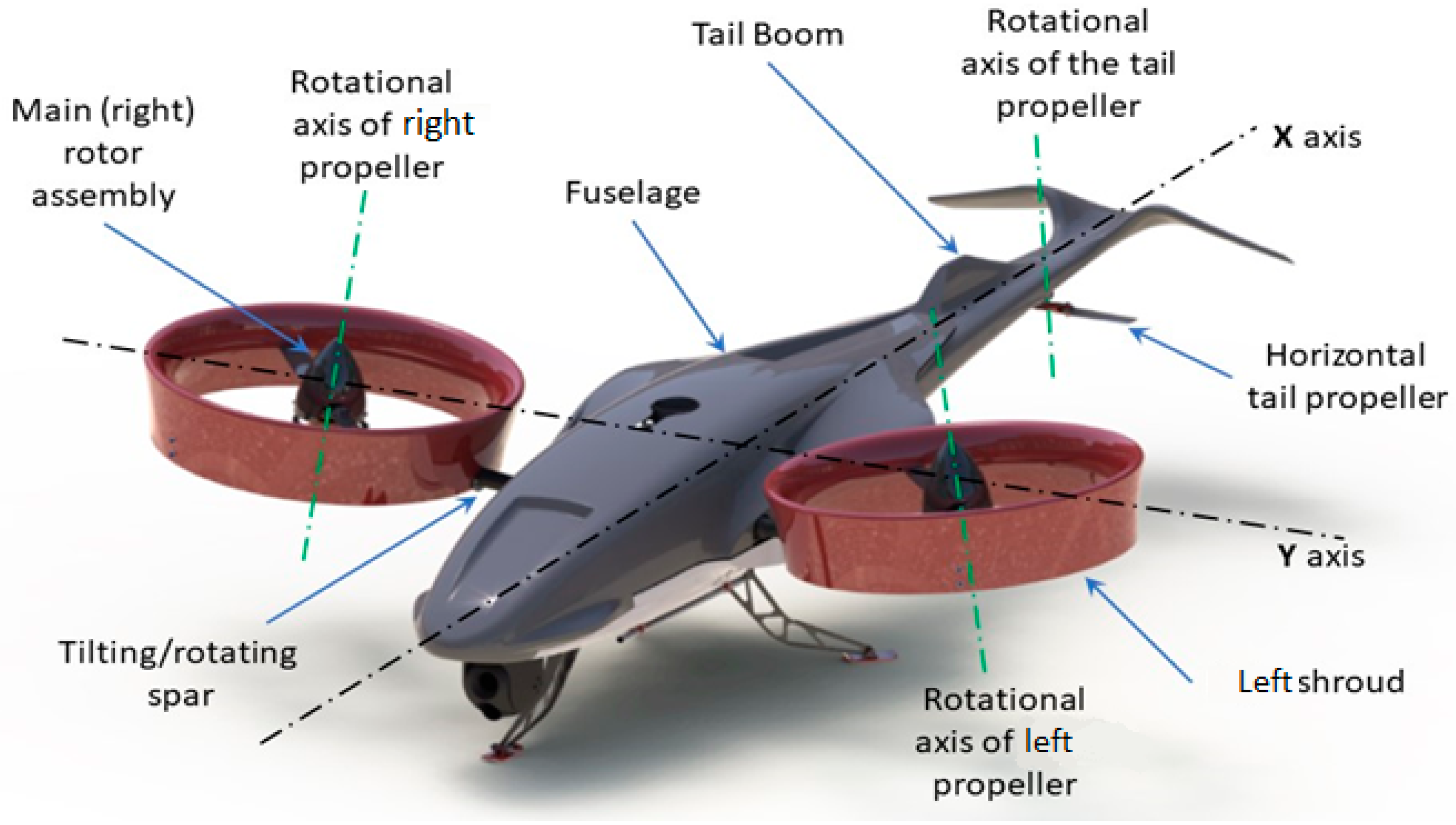
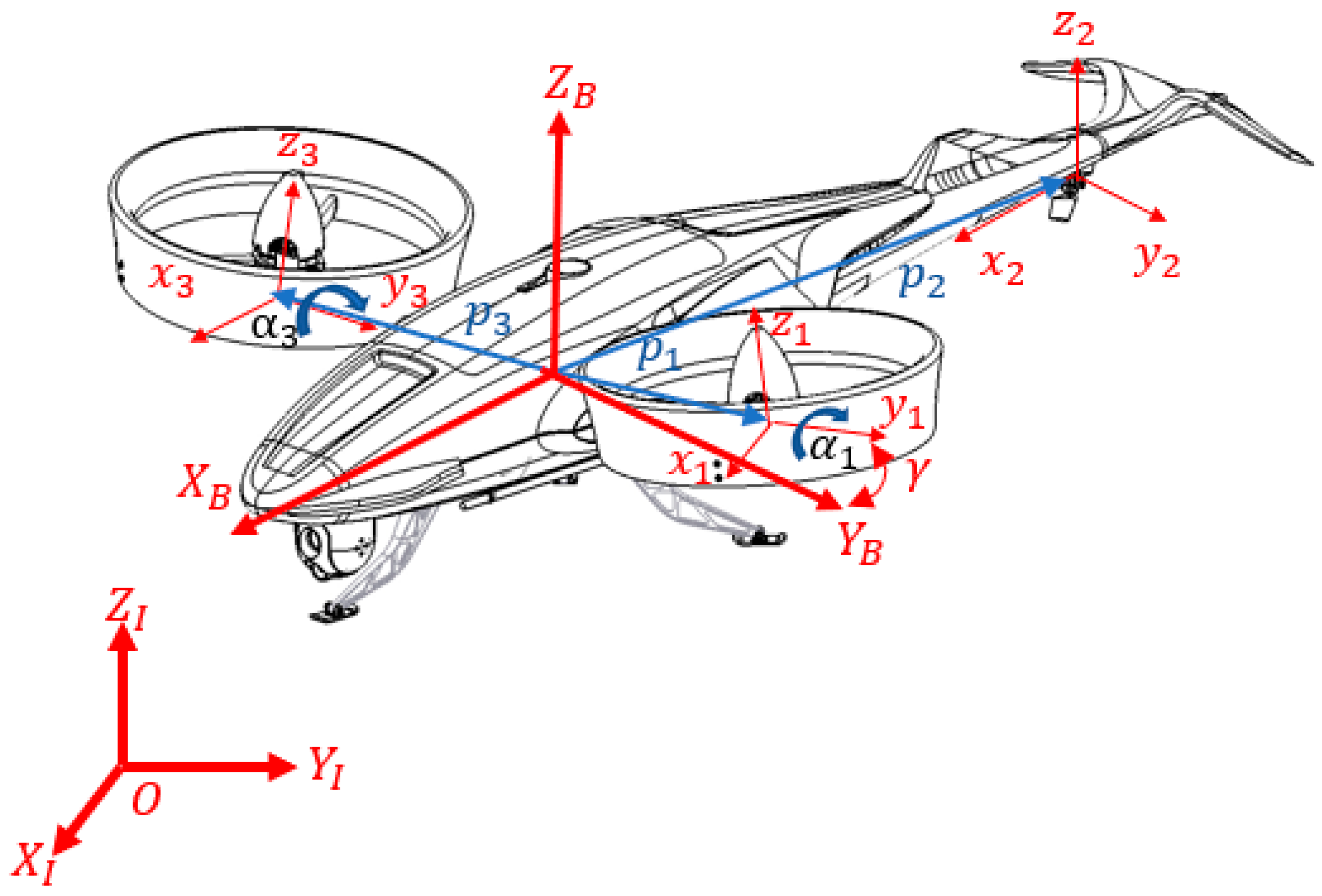
The following sections of this paper are organized as follows: the nonlinear mathematical model of the aircraft of interest (termed the Navig8) is described in Section 3; the proposed dynamic inversion control method is described in Section 4, while Section 5 presents illustrative numerical simulations showing the performance of the proposed controller, followed by the conclusions in Section 6.

3. Aircraft’s Dynamic Model

3.1. Flight Mechanism

The drone under consideration in this paper is a six degrees of freedom (DOF) tilt rotorcraft. Each of the aircraft’s ducted or shrouded propellers which rotate in opposite directions have independent tilt angles, speed, and variable pitch angles. The aircraft also has a variable pitch propeller (VPP) tail rotor, which, in contrast to helicopters, produces thrust perpendicular to the horizontal reference plane of the aircraft, enabling the aircraft to perform pitch maneuvers (Figure 1).

The thrust produced by each of the three propellers can be independently controlled in three possible ways: (i) by changing the propeller’s rotational speed (${\omega }_1,{\omega }_2,$ and ${\omega }_3$), (ii) by changing the propeller’s angle of attack (${\beta }_1,{\beta }_2,$ and ${\beta }_3$), and (iii) a combination of “i” and “ii” (a combination of propeller rpm and VPP changes) via the control signals ${\omega }_1,{\omega }_2,{\omega }_3,{\beta }_1,{\beta }_2,$ and ${\beta }_3$, which correspond to the propellers’ speed and the angle of attack of the left, tail, and right propellers, respectively. Additionally, each of the two main (left and right) propellers can independently tilt by an angle ${\alpha }_i$, providing the capability for thrust vectoring. These characteristics result in the use of eight control signals (${\omega }_i,{\alpha }_i,$ and ${\beta }_i$), which provides the opportunity to control the aircraft in different ways via proper control allocation mechanisms. Optimal control allocation would also enable the aircraft to cope with internal failures (e.g., damage of the ${rpm}_i$ control) under a high reaction time in diverse ways. Due to the control allocation challenges that are available for the control of such an UAV, in this paper, we only considered controlling the thrust produced by each of the UAV’s propellers via option “i” (i.e., keeping all ${\beta }_i$ parameters unchanged throughout the given mission). Controlling the UAV via options “ii” and “iii” will be the subject of a subsequent paper focusing on the corresponding control allocation formulations needed to determine the optimal use of the propellers’ rpm, VPP, or a combination of both. As a result of the reduced control complexities employed in this paper, the UAV was left with five control inputs: ${\omega }_1,{\omega }_2,{\omega }_3,{\alpha }_1$, and ${\alpha }_3$. In order to minimize the adverse aerodynamic ground and wall effects, which the UAV would experience when flying close to surfaces (e.g., ground), the two main propellers were set to have a constant dihedral angle, $\gamma$, (see Figure 2). Such a dihedral angle was determined from extensive CFD (computational fluid dynamics) analysis [32].

The combination of the above-mentioned characteristics enables the aircraft to perform untypical flight maneuvers that other aircraft cannot execute, including pitch hover at angles within the range from −90° (nose down) to 90° (nose up). With effective control and mechanical design changes, these flight characteristics can be augmented to perform enhanced maneuvers, such as perching and inverted pitch hover maneuvers suitable for time-extended surveillance, as well as other critical missions inside dynamic cluttered spaces.

The drone, having a mass “m”, can fly sideways, forwards, and backwards in diverse attitudes using the five control inputs that were considered in this paper. The sideways motion (in the vehicle’s “y” direction—see Figure 2) was achieved through generating a differential thrust/speed of the two (left and right) main (shrouded) propellers. The tilt angles, ${\alpha }_1$ and ${\alpha }_3$, of such propellers were changed in equal amounts to achieve fore and aft motions (i.e., motion in the “x” direction). Tilting the angle of the propellers in opposite directions created the yaw motion (rotation about the vehicle’s “z” axis). The described motions are, however, highly coupled, that is, requesting the aircraft to execute a given maneuver produces a side effect (sometimes undesirable) motion. Such coupled motions have been summarized in

Table 1. Motions and respective coupling effects.

Motion		Surge	Sway	Heave	Roll	Pitch	Yaw
Translation	Surge (front/back)	-				X	X
	Sway (side-to-side)		-		XX		XX
	Heave (up/down)	X		-		X
Rotation	Roll				-	X	XXX
	Pitch	XXX		XX		-	XX
	Yaw		X	X	X		-

, where the number of Xs in each box denotes the degree of the corresponding coupled motions. For example, if the aircraft has been requested to execute a pure sideways (translational) motion, the differential rotational speeds of the main propellers needed to achieve such a motion also generate roll and yaw aircraft motions. Such coupled motions and the number of simultaneous motion(s) associated with the given (desired) motion have been described via the drone’s mathematical model.

3.2. Dynamic Model

The Newton–Euler formulation was used to derive the system’s dynamic model. Two frames of reference were used: an inertial reference frame, denoted by ${OX}_I{Y}_I{Z}_I$, and a body reference frame positioned at the center of mass of the UAV, denoted by ${OX}_b{Y}_b{Z}_b$, as shown in Figure 2.

In order to describe the rotation of the drone, the Euler angles (roll (ϕ), pitch (θ), and yaw (ψ)) were used and, therefore, the transformation matrix from the inertial to the body reference frame was defined by Equation (1) as:

$$R_I^B=\left[\begin{array}{c}c\theta c\psi c\theta s\psi -s\theta \\ -c\varphi s\psi +s\varphi s\theta c\psi c\varphi c\psi +s\varphi s\theta s\psi s\varphi c\theta \\ s\varphi s\psi +c\varphi s\theta c\psi -s\varphi c\psi +c\varphi s\theta s\psi c\varphi c\theta \end{array}\right]$$

(1)

where c and s represent the cos and sin functions of the corresponding angle (e.g., $c\varphi =\mathrm{c}\mathrm{o}\mathrm{s}\varphi$), respectively. The matrix describing the relationship between the body’s angular velocity (p, q, or r) and the rotational speed of the Euler angles was defined as per Equation (2):

$$\mathit{\omega }=\left[\dot{\begin{array}{c}\varphi \\ \dot{\begin{array}{c}\theta \\ \dot{\psi }\end{array}}\end{array}}\right]=\left[\begin{array}{c}1tan\theta sin\varphi tan\theta cos\varphi \\ 0cos\varphi -sin\varphi \\ 0sin\varphi /cos\theta cos\varphi /cos\theta \end{array}\right]\left[\begin{array}{c}p\\ q\\ r\end{array}\right]=J\left(\vartheta \right)\Omega$$

(2)

Due to the complexities related to the operational capabilities of the Navig8 UAV, the following three assumptions (Ak) and two constraints (Ck) were made to simplify the drone’s equations of motion:

• The body reference frame and the aircraft center of mass are coincident.
• The aircraft’s structure is symmetric to its XZ (longitudinal) plane, resulting in $I_{XY}=I_{ZY}=0$.
• All aerodynamic coefficients, such as drag and lift, remain constant throughout the given flight mission.
• The thrust, $T_i^{}$, generated by propeller I, is proportional to the square of its rotational speed.
• The trust and torque coefficients for each of the three propellers (i = 1, 2, or 3) is assumed constant, as described by Equations (3) and (4).

$$T_i^j={\left[\begin{array}{ccc}0& 0& k_{T_i}{{\omega }_i}^2\end{array}\right]}^T$$

(3)

$${\tau }_i^j={\left[\begin{array}{ccc}0& 0& K_{{To}_i}{{\omega }_i}^2\end{array}\right]}^T$$

(4)

and

$$k_{T_i}=\frac{1}{2}{C}_{T_i}\rho A_i{r_i}^2$$

$$K_{{To}_i}=\frac{1}{2}{C}_{{To}_i}\rho A_i{r_i}^3$$

where $C_T$ and $C_{To}$ represent the propellers’ trust and torque coefficients, $r$ and $A$ specify the radius and footprint area of each propeller, and $\rho$ denotes the air density.

Based on the previously mentioned aspects, the equations of the motion for the Navig8 can be expressed as Equation (5).

$$\left\{\begin{array}{c}\ddot{x}=\frac{1}{m}\left(X_{b}c\theta c\psi +Z_b\left(s\varphi S\psi +c\varphi s\theta c\psi \right)\right)\\ \ddot{y}=\frac{1}{m}\left(X_{b}c\theta s\psi +Z_b\left(-s\varphi c\psi +c\varphi s\theta s\psi \right)\right)\\ \ddot{z}=\frac{1}{m}\left(-X_{b}s\theta +Z_{b}c\varphi c\theta \right)-g\\ \dot{p}=\frac{I_{XZ}}{I_{XX}}\left(\dot{r}+pq\right)+\frac{I_{YY}-I_{ZZ}}{I_{XX}}qr+\frac{L}{I_{XX}}\\ \dot{q}=\frac{I_{XZ}}{I_{YY}}\left(r^2-p^2\right)+\frac{I_{ZZ}-I_{XX}}{I_{YY}}pr+\frac{M}{I_{YY}}\\ \dot{r}=\frac{I_{XZ}}{I_{ZZ}}\left(\dot{p}-qr\right)+\frac{I_{XX}-I_{YY}}{I_{ZZ}}pq+\frac{N}{I_{ZZ}}\end{array}\right.$$

(5)

The terms $X$, $Y$, $Z$, $L$, $M$, and $N$ in Equation (5) denote the total forces and torques in the $x$, $y$, and $z$ directions, respectively. Such terms were obtained as per Equation (6):

$$\left[\begin{array}{c}L\\ M\\ N\\ X\\ Z\end{array}\right]=\left[\begin{array}{c}\begin{array}{c}{k}_{T1}b\cos \gamma \\ {-k}_{T1}a\cos \gamma \\ k_{To1}\cos \gamma \end{array}\begin{array}{c}-k_{To1}\\ {-k}_{T1}c\\ k_{T1}b\end{array}\begin{array}{c}-k_{T3}b\cos \gamma \\ -k_{T3}a\cos \gamma \\ -k_{T03}\cos \gamma \end{array}\begin{array}{c}{k}_{To3}\\ -k_{T3}c\\ -k_{T3}b\end{array}\begin{array}{c}0\\ k_{T2}d\\ k_{To2}\end{array}\\ \begin{array}{c}0\\ k_{T1}\cos \gamma \end{array}\begin{array}{c}-k_{T1}\\ 0\end{array}\begin{array}{c}0\\ k_{T3}\cos \gamma \end{array}\begin{array}{c}{-k}_{T3}\\ 0\end{array}\begin{array}{c}0\\ k_{T2}\end{array}\end{array}\right]\left[\begin{array}{c}{\mathsf{\omega }}_1^2\cos {\alpha }_1\\ {\mathsf{\omega }}_1^2\sin {\alpha }_1\\ {\mathsf{\omega }}_3^2\cos {\alpha }_3\\ {\mathsf{\omega }}_3^2\sin {\alpha }_3\\ {\mathsf{\omega }}_2^2\end{array}\right]$$

(6)

where $a$, $b$, $c$, $d$, and $e$ represent the corresponding orthogonal distances between the center of mass of the UAV and the left, right, and back propellers described by the vectors $p_1=\left(a,b,c\right), p_2=\left(-d,0,-e\right),$ and $p_3=\left(a,-b,c\right)$, respectively, as illustrated in Figure 2. The five expressions provided in Equation (6), $X$, $Z$, $L$, $M$, and $N$, define a coupled set of equations, which are simplified by defining the five control variables $u_1,u_2,u_3,u_4,$ and $u_5$, as per Equation (7).

$$\mathrm{U}=\left[\begin{array}{c}{u}_1\\ u_2\\ u_3\\ u_4\\ u_5\end{array}\right]=\left[\begin{array}{c}{\mathsf{\omega }}_1^2\cos {\alpha }_1\\ {\mathsf{\omega }}_1^2\sin {\alpha }_1\\ {\mathsf{\omega }}_3^2\cos {\alpha }_3\\ {\mathsf{\omega }}_3^2\sin {\alpha }_3\\ {\mathsf{\omega }}_2^2\end{array}\right]$$

(7)

It is worthwhile to clarify that based on the assumptions and the drone’s symmetrical geometry, the expression for $Y$ is not involved in Equation (6). As a result, Equation (6) can be rewritten as Equation (8):

$$\left[\begin{array}{c}L\\ M\\ N\\ X\\ Z\end{array}\right]=\left[\begin{array}{c}\begin{array}{c}{k}_{T1}b\cos \gamma \\ {-k}_{T1}a\cos \gamma \\ k_{To1}\cos \gamma \end{array}\begin{array}{c}-k_{To1}\\ {-k}_{T1}c\\ k_{T1}b\end{array}\begin{array}{c}-k_{T3}b\cos \gamma \\ -k_{T3}a\cos \gamma \\ -k_{T03}\cos \gamma \end{array}\begin{array}{c}{k}_{To3}\\ -k_{T3}c\\ -k_{T3}b\end{array}\begin{array}{c}0\\ k_{T2}d\\ k_{To2}\end{array}\\ \begin{array}{c}0\\ k_{T1}\cos \gamma \end{array}\begin{array}{c}-k_{T1}\\ 0\end{array}\begin{array}{c}0\\ k_{T3}\cos \gamma \end{array}\begin{array}{c}{-k}_{T3}\\ 0\end{array}\begin{array}{c}0\\ k_{T2}\end{array}\end{array}\right]\left[\begin{array}{c}{u}_1\\ u_2\\ u_3\\ u_4\\ u_5\end{array}\right]=KU$$

(8)

in which $K$ is a fixed matrix defined by the physical characteristics of the UAV, as per Equation (8). Therefore, the control signals vector, $\mathrm{U}$, can be calculated if the inverse of $K$ exists, as represented by Equation (9) below.

$$\mathrm{U}=\left[\begin{array}{c}{u}_1\\ u_2\\ u_3\\ u_4\\ u_5\end{array}\right]=K^{-1}\left[\begin{array}{c}L\\ M\\ N\\ X\\ Z\end{array}\right]$$

(9)

Therefore, considering Equation (7), the five control inputs of interest are computed per Equation (10) as:

$$\left[\begin{array}{c}{\omega }_1^2\\ {\omega }_3^2\\ {\omega }_2^2\\ {\alpha }_1\\ {\alpha }_3\end{array}\right]=K^{-1}\left[\begin{array}{c}\sqrt{u_1^2+u_2^2}\\ \sqrt{u_3^2+u_4^2}\\ u_5\\ {\tan }^{-1}\frac{u_2}{u_1}\\ {\tan }^{-1}\frac{u_4}{u_3}\end{array}\right]$$

(10)

4. Control Technique

The UAV’s dynamic model can be represented in generic form of a nonlinear state-space system:

$$\dot{\mathit{x}}=F(\mathit{x},\mathit{u})$$

(11)

where ${\mathit{x}}_t$ and ${\mathit{u}}_t$ represent the state and input transpose vectors, at time $t$, respectively:

$${\mathit{x}}_t={\left[x,y,z,\phi ,\theta ,\psi ,\dot{x},\dot{y},\dot{z},\dot{\phi },\dot{\theta },\dot{\psi }\right]}^{\prime }$$

$${\mathit{u}}_t={\left[{\omega }_1,{\omega }_2,{\omega }_3,{\alpha }_1,{\alpha }_3,{\beta }_1,{\beta }_2,{\beta }_3\right]}^{\prime }$$

By calculating the first-order Taylor series of Equation (11), Equation (11) can be written as:

$$\dot{\mathit{x}}={\dot{\mathit{x}}}_0+\frac{\partial F}{\partial \mathit{x}}{|}_{{\mathit{x}}_0,{\mathit{u}}_0}\left(\mathit{x}-{\mathit{x}}_0\right)+\frac{\partial F}{\partial \mathit{u}}{|}_{{\mathit{x}}_0,{\mathit{u}}_0}\left(\mathit{u}-{\mathit{u}}_0\right)$$

(12)

in which ${\mathit{x}}_0$ and ${\mathit{u}}_0$ represent the state and input vectors of the system at the previous time step, (${\mathit{t}}_0$), respectively. An INDI description of a system described by Equation (12) is possible under the following two assumptions:

6.

The state of the UAV and input, $\mathit{u}$, are bounded, and the function $F$ is continuous.

7.

The amount of time that has passed between ${\mathit{x}}_0$ and $\mathit{x}$ (sampling time) is sufficiently small.

By using a small sampling time (assumption b) and employing high performance actuators in the drone, the changes in the state of the UAV ($∆\mathit{x}$) with the given time step can be considered negligible (i.e., $∆\mathit{x}=\mathit{x}-{\mathit{x}}_0$) with respect to the large changes in the input parameters represented as ($∆\mathit{u}=\mathit{u}-{\mathit{u}}_0$), given that state changes arise as a result of the integration of input changes and are, therefore, slower.

The assumptions listed above imply that the difference ($\mathit{x}-{\mathit{x}}_0$) can be considered negligible (ignored) and therefore, Equation (12) becomes:

$$\dot{\mathit{x}}={\dot{\mathit{x}}}_0+\frac{\partial F}{\partial \mathit{x}}{|}_{{\mathit{x}}_0,{\mathit{u}}_0}\left(\mathit{x}-{\mathit{x}}_0\right)+\frac{\partial F}{\partial \mathit{u}}{|}_{{\mathit{x}}_0,{\mathit{u}}_0}\left(\mathit{u}-{\mathit{u}}_0\right)$$

(13)

To be efficient, this INDI approach requires a suitable timescale separation, which was considered as 0.01 s in this paper. To achieve the required timescale separation, the approach taken in this paper was to employ a combination of NDI, INDI, and PID controllers, forming an inner and outer loop control strategy, as illustrated in Figure 3.

The developed control architecture can be applied to diverse aircraft systems, especially those with complex dynamics operating in the presence of internal (e.g., system failures) and/or external disturbances (e.g., wind gusts). Overall, the controller would receive, as a control input, a desired path/trajectory to follow, which includes the desired position ($x_d,y_d,z_d$), orientation (${\varphi }_d,{\theta }_d,{\psi }_d$), and time conditions, defining the UAV’s maneuvers from where the required control signals will be computed.

4.1. The Attitude Controller (INDI)

For the INDI attitude controller, the state of the drone was defined as a subset of the state variables used in Equation (11). Such a subset, $\overline{x}\in x$, comprises the roll, pitch, and yaw Euler angles and the corresponding rotational speeds $(p,q,\mathrm{and}r)$, as described by Equation (14), where $\vartheta ={\left[\varphi ,\theta ,\psi \right]}^T$, $\mathsf{\Omega }={\left[p,q,r\right]}^T$, and $\overline{u}={\left[u_1,u_2,u_3\right]}^T$ have been defined based on Equations (8) and (9) and the dynamic equations of the system (e.g., Equation (5)):

$$\overline{x}=\left[\begin{array}{c}\vartheta \\ \mathsf{\Omega }\end{array}\right]=\left[\begin{array}{c}\varphi \\ \theta \\ \psi \\ p\\ q\\ r\end{array}\right]\overline{u}=\left[\begin{array}{c}{u}_1\\ u_2\\ u_3\end{array}\right]$$

(14)

It is important to note that the lateral (sway) motion of the UAV is highly coupled with the roll angle of the body (see Table 1). The result of such coupled motions is that the UAV cannot perform pure lateral movement without rolling and vice versa. The additional coupled effects, as represented in Table 1, are manageable and can be decoupled and be precisely controlled. Therefore, for the proposes of this paper, the roll angle was not considered as a controllable state, but it was used as an input to reach a desired lateral translation.

From Equation (14), one can map the state vector, $\overline{x}$, to the Euler angles of the UAV, $\vartheta$, via a transformation matrix $H$, as per Equation (15):

$$\vartheta =H\overline{x}=\left[I_{3\times 3}{0}_{3\times 3}\right]\overline{x}$$

(15)

Since the first-order time derivative of the control variable vector, $\vartheta ={\left[\varphi ,\theta ,\psi \right]}^T$, is not directly related to the control input vector, $\overline{u}$, the relationship between the input and output variables was determined through obtaining the second-order derivative of the control vector, $\vartheta$, as shown in Equations (16) and (17):

$$\dot{\vartheta }=\frac{d\vartheta }{dt}=\frac{dH\overline{x}}{dt}=H\dot{\overline{x}}=H\left[\begin{array}{c}\mathit{\omega }\\ \dot{\mathit{\omega }}\end{array}\right]=J\left(\vartheta \right)\Omega$$

(16)

$$\ddot{\vartheta }=\frac{d^2\vartheta }{{dt}^2}=\frac{d\left(J\left(\vartheta \right)\Omega \right)}{dt}=\frac{d}{d\overline{x}}\left(\left[\begin{array}{c}1tan\theta sin\varphi tan\theta cos\varphi \\ 0cos\varphi -sin\varphi \\ 0sin\varphi /cos\theta cos\varphi /cos\theta \end{array}\right]\left[\begin{array}{c}p\\ q\\ r\end{array}\right]\right)\dot{\overline{x}}$$

(17)

Considering Equation (17) and the dynamic equations of the UAV, Equations (5)–(7), one can define $\ddot{\vartheta }$ as a function of $\overline{x}$ and $\overline{u}$, as shown in Equation (18). From this formulation, and following Equation (11), the INDI controller can be formulated by performing a Taylor series expansion in the current time step, $t$, as described in Equation (19):

$$\ddot{\vartheta }=F_{\vartheta }\left(\overline{x},\overline{u}\right)$$

(18)

$$\ddot{\vartheta }\simeq F\left({\overline{x}}_0,{\overline{u}}_0\right)+\frac{\partial F_{\vartheta }\left(\overline{x},u\right)}{\partial \overline{x}}{|}_{{\overline{x}}_0,u_0}\left(\overline{x}-{\overline{x}}_0\right)+\frac{\partial F_{\vartheta }\left(\overline{x},\overline{u}\right)}{\partial \overline{u}}{|}_{{\overline{x}}_0,{\overline{u}}_0}\left(\overline{u}-{\overline{u}}_0\right)$$

(19)

Using $F\left({\overline{x}}_0,{\overline{u}}_0\right)={\ddot{\vartheta }}_0$ as the angular acceleration measurement of the UAV at the previous time step, $t-1$, a very short measurement sampling time ($∆t$) can be used, given that the actuator dynamics are faster (as per assumption b). Then, it is reasonable to further consider $\left(\overline{x}-{\overline{x}}_0\right)\approx 0$ when compared to the changes in the control output, $∆\overline{u}=\left(\overline{u}-{\overline{u}}_0\right)$. In these circumstances, the simplified expression shown in Equation (20) can be used to obtain the control law:

$$\ddot{\vartheta }={\ddot{\vartheta }}_0+K\left({\overline{x}}_0,{\overline{u}}_0\right)∆\overline{u}$$

(20)

Solving for $∆\overline{u}$ from Equation (20) results in $∆\overline{u}={K({\overline{x}}_0,{\overline{u}}_0)}^{-1}(\ddot{\vartheta }-{\ddot{\vartheta }}_0)$, where the matrix $K\left({\overline{x}}_0,{\overline{u}}_0\right)$ represents the partial derivative matrix of function $F_{\vartheta }$ with respect to the control inputs of the system, $\overline{u}$, resulting in:

$$K\left({\overline{x}}_0,{\overline{u}}_0\right)=J\left({\overline{x}}_0\right)\left[\begin{array}{ccc}\frac{k_{T1}b\cos \gamma }{I_{XX}}& 0& 0\\ 0& \frac{{-k}_{T1}c}{I_{YY}}& 0\\ 0& 0& \frac{-k_{T03}\cos \gamma }{I_{ZZ}}\end{array}\right]$$

(21)

With the above formulations, it is possible to effectively compute the control inputs (i.e., $L,M,\mathrm{and}N$) based on the vehicle’s angular acceleration measurements taken at time step $t-1$. Thus, Equations (20) and (21) represent the attitude (orientation) INDI controller, which guides the UAV on how to attain the desired orientation at a given position $(x,y,\mathrm{or}z)$ when following a desired path. As a result, the desired orientation behavior of the aircraft was not significantly affected when the slower dynamics of the model were ignored (which will be described in Section 6).

4.2. The Position Controller (NDI + INDI)

The controller designed to control the aircraft’s orientation (i.e., yellow boxes in Figure 3), provides the torques $(L,M,\mathrm{and}N)$ required to orient the aircraft. Such torques can then be used in combination with the forces $\left(X\mathrm{and}Z\right)$ needed to position the aircraft at a specific point $(x,y,\mathrm{or}z)$ to generate the control signals needed to maneuver the UAV. As illustrated in Figure 3, a position controller must be formulated to provide such forces that will enable the UAV to track the desired path, which includes the position and orientation information. The aircraft’s translational movement control was achieved via a combination of an NDI and INDI (INDI + NDI) control strategy (blue boxes shown in Figure 3), where the NDI port is responsible for controlling the lateral motion, while the INDI port focuses on computing the $X$ and $Z$ forces that need to be applied to the aircraft through the control of the propeller’s thrust vectoring ability. Such a strategy enables to manage the coupled motions of the aircraft described in Table 1. Specifically, the proposed controller was targeted to reduce the coupled translational motions taking place in the $x-z$ (longitudinal) plane of the aircraft. That is, the position controller aimed to decouple the surge and heave motions of the aircraft. An NDI controller was employed for the lateral (sway) movement, and an INDI controller was developed for the movements in the $x-z$ directions (heave). For altitude regulation in the $x-z$ plane, the control inputs $u_4$ and $u_5$ were used. However, there was no direct control input within the vector $\mathrm{U}$ (Equation (7)) for the side movement. Thus, a differential thrust/speed of the propellers was used to provide the required lateral motion. Therefore, finding the required roll angle, $\varphi$, was required to generate the desired lateral motion in terms of the aircraft’s $y$ position and its rate of change, $\dot{y}$. In turn, the computed roll angle was provided as one of the three inputs for the attitude controller. To enable the NDI controller to cope with disturbances (in the $y$ direction), a sigma-pi neural network (NN) adaptive compensator was used to correct modeling errors and overcome the tendency of NDI controllers to be sensitive to the dynamic model’s accuracy [28,33].

The INDI position controller for the $x$ and $z$ aircraft motions was developed using a similar approach of the attitude controller (Section 4.1). For the position controller, however, a two-layer architecture was used. An INDI formulation was used to cancel the non-linearities associated with the linear dynamics of the system and generate the control signals for the $x$ and z positions of the UAV. In addition, NDI was employed for the lateral (position) motion.

4.2.1. The Position INDI Controller

For the position INDI controller, a virtual control variable, $\widehat{u}$, defined as per Equation (22), was used.

$$\widehat{u}=\left[\begin{array}{c}X\\ Z\end{array}\right]$$

(22)

Considering the dynamic model of the system in the $x-z$ direction, Equation (23), and defining the states variables $x$ and $z$ as vector $\widehat{x}$, the second-order time derivative of matrix $\widehat{x}$ for the INDI position controller was given as per Equation (25):

$$\left[\ddot{\begin{array}{c}x\\ \ddot{z}\end{array}}\right]=\left[\begin{array}{c}0\\ -g\end{array}\right]+\frac{1}{m}\left[\begin{array}{c}c\theta c\psi s\varphi s\psi +c\varphi s\theta c\psi \\ -s\theta 0\end{array}\right]\left[\begin{array}{c}{X}_b\\ Z_b\end{array}\right]$$

(23)

$$\widehat{x}=\left[\begin{array}{c}x\\ z\end{array}\right]$$

(24)

$$\ddot{\widehat{x}}\simeq {\ddot{\widehat{x}}}_0+\frac{\partial }{\partial u}\left(f_P\left(\widehat{x},\widehat{u}\right)\right){|}_{\widehat{x}={\widehat{x}}_0,\widehat{u}={\widehat{u}}_0}\left(\widehat{u}-{\widehat{u}}_0\right)={\ddot{\widehat{x}}}_0+G({\widehat{x}}_0,{\widehat{u}}_0)\mathsf{\Delta }\widehat{u}$$

(25)

in which $G\left({\widehat{x}}_0,{\widehat{u}}_0\right)$ is defined by Equation (26).

$$G\left({\widehat{x}}_0,{\widehat{u}}_0\right)=\frac{\partial }{\partial u}\left(f_P\left(\widehat{x},\widehat{u}\right)\right){|}_{\widehat{x}={\widehat{x}}_0,\widehat{u}={\widehat{u}}_0}=\frac{1}{m}\left[\begin{array}{c}c\theta c\psi s\varphi s\psi +c\varphi s\theta c\psi \\ -s\theta c\varphi c\theta \end{array}\right]$$

(26)

$$u=u_0+{G\left({\widehat{x}}_0,{\widehat{u}}_0\right)}^{-1}(\ddot{\widehat{x}}-{\ddot{\widehat{x}}}_0)$$

(27)

4.2.2. The Position NDI Controller

As previously mentioned, due to the high coupling between the roll angle, $\varphi$, and the position in the y direction, it is not possible to independently control both parameters at the same time. Thus, a variable, $u_y$, (Equation (28)) was defined, which enables the design of an NDI controller to control the UAV’s lateral motion. The output of this controller block, ${\varphi }_d$, was fed to the attitude control block, which will control the lateral motion of the drone.

$$u_y=sin\varphi$$

(28)

Following the process used in Section 4.1, the second-order time derivative of the side motion of the drone’s mathematical model, $y$, for the NDI position controller used the corresponding formulation in Equation (5), where the term $sin\varphi$ has been replaced with $u_y$, as shown in Equation (29):

$$\ddot{y}=\frac{1}{m}\left(X_{b}c\theta s\psi +Z_b\left(-u_{y}c\psi +c\varphi s\theta s\psi \right)\right)=f\left(\vartheta \right)+g\left(\vartheta \right)u_y$$

(29)

A virtual control input, $v$, can then be chosen as $v=\ddot{y}$ if $\mathit{det}(g\left(\theta \right))\ne 0$.

$$u_y={g\left(\vartheta \right)}^{-1}(v-f(\vartheta \left)\right)$$

(30)

$$g\left(x,u\right)=\frac{-Z_b}{C\psi }$$

(31)

An accurate description of the functions $f$ and $g$ within Equation (30) was required to cancel all model uncertainties and cross-couplings in the system. However, an exact cancelation of nonlinearities is practically impossible. Therefore, a sigma-pi neural network (NN) was used to compensate the uncertainties. Such a NN is represented as a NN adaptive compensator in Figure 3, which processes nine inputs (i.e., $x_0,y_0,z_0,x_d,z_d,e,v_{ad},X,\mathrm{and}Z)$ plus a set of three Kronecker values $(c_1,c_2,c_3)$ (defined later in this document in Equation (37)), where $x_0,y_0$, and $z_0$ represent the position of the UAV in the previous time step, and $e=y_{rm}-y_0$ defines the error between the reference model and the lateral position of the UAV in the previous time step. From the defined error and the Kronecker values, the sigma-pi NN generates $v_{ad}$, which adaptively compensates the input produced via the NDI controller, which operates under the assumption that the mathematical model of the system is accurate.

As a result, the sigma-pi NN compensates the inversion error with a real-time pseudo control signal, $v_{ad}$, where the pseudo control command was generated as per Equation (32):

$$v=v_{rm}+v_{pd}-v_{ad}$$

(32)

where $v_{rm}=\ddot{y}$ is the reference model’s pseudo control, and $v_{pd}$ is the signal generated via a PD linear regulator (see Section 4.3), which is used to regulate the dynamic response of the system as per Equation (33):

$$v_{pd}=k_p\left(y_{rm}-y_0\right)+k_d\left({\dot{y}}_{rm}-{\dot{y}}_0\right)$$

(33)

As a result, the dynamics of the model tracking error can then be described via Equation (34):

$$\dot{\epsilon }=A\epsilon +B\left(v_{ad}-∆\right)$$

(34)

where $\epsilon =\left[\begin{array}{c}{y}_{rm}-y\\ {\dot{y}}_{rm}-\dot{y}\end{array}\right],A=\left[\begin{array}{c}01\\ -k_p-k_d\end{array}\right]$, and B = $\left[\begin{array}{c}0\\ 1\end{array}\right].$

4.2.3. The Sigma-Pi Neural Network

In comparison to other neural networks, the sigma-pi NN [33] uses summation and quadrature neurons in its hidden layers, providing the ability to preserve the network’s highly nonlinear mapping capability [34]. Figure 4 depicts the single layer sigma-pi NN used in the proposed UAV controller as having three inputs and one output.

The neural network’s input/output map can be expressed as follows:

$$v_{ad}=\sum _{j=1}^k{w}_j{\beta }_j=W^T\beta$$

(35)

where $W^T$ represents the weight coefficient matrix, and $\beta$ denotes the basis function vector, which is defined as per Equation (36):

$$\beta =kron(kron\left(c_1,c_2\right),c_3)$$

(36)

The “$kron$” denotes the Kronecker product operating on $c_1,c_2,$ and $c_3$, which are defined as follows:

$$\left\{\begin{array}{l}{c}_1={\left[0.1e{e}^2\right]}^T\\ c_2={\left[0.01x_d{y}_d{z}_{d}XYZ\right]}^T\\ c_3={\left[x_0{y}_0{z}_0\right]}^T\end{array}\right.$$

(37)

The corresponding weight error can then be expressed as follows:

$$\tilde{W}=W-W^{*}$$

(38)

where $W^{\mathrm{*}}$ denotes the ideal set of weights. Thus, the model tracking error (Equation (34)) was written as per Equation (39), and the update law for the NN was expressed via Equation (40).

$$\dot{e}=Ae+B{\tilde{W}}^T\zeta +B({\tilde{W}}^T\zeta -\Delta )$$

(39)

$${\dot{\tilde{W}}}_j\left(t\right)=\left\{\begin{array}{cc}-{\Gamma }_j\left(e^T{P}_{j}B\right){\zeta }_j& for{‖e_j‖}_{P_j}>{e_0}_j\\ 0& for{‖e_j‖}_{P_j}<{e_0}_j\end{array}\right.$$

(40)

The terms in Equation (40) are defined as ${‖e_j‖}_{P_j}=\sqrt{{e^T}_j{P}_j{e}_j}$. ${\mathsf{\Gamma }}_j$ is a positive constant adaptation gain (learning rate), and $P_j$ is a symmetric, positive definite matrix satisfying the Lyapunov equation $P_j{A}_j+{A_j}^T{P}_j=-I$ for the linear system error with NN weights. The Hurwitz matrix $A_j$ of Equation (37) ensures the existence of a unique $P_j=P_j^T>0$, where the $P_j$ matrix used in the developed controller is described as per Equation (41):

$$P_j=\left[\begin{array}{cc}\frac{K_{d_j}}{2K_{p_j}}+\frac{K_{p_j}}{2K_{d_j}}(1+\frac{1}{K_{p_j}})& \frac{1}{2K_{p_j}}\\ \frac{1}{2K_{p_j}}& \frac{1}{2K_{d_j}}(1+\frac{1}{K_{p_j}})\end{array}\right].$$

(41)

The NDI + NN outer loop controller responsible for the slow dynamics of the UAV’s $y$ channel generates the state command for the inner INDI block as per Equation (42):

$${\phi }_d={\mathit{sin}}^{-1}(u_y).$$

(42)

4.3. The PD/PID Controller

The altitude and position controllers described above, Equations (20), (27), and (30), were designed based on the second derivative of the position and attitude states of the UAV, meaning that the controller has been developed to follow the second-order derivative of the desired trajectory (acceleration) of the aircraft. Therefore, in order to enable the UAV to follow the desired position/attitude (trajectory), three proportional derivative (PD) controllers for attitude (i.e., ${PD}_{\varphi }$, ${PD}_{\theta }$, and ${PD}_{\psi }$) and three PID controllers (i.e., ${PID}_x$, ${PID}_y$, and ${PID}_z)$ for position were used to map the pose error (the difference between the desired and measured poses in the previous time step) [28]. Similar to that conducted by the authors of [28], the PD/PID gains were optimized using a non-dominated, sorting-based multi-objective evolutionary algorithm (MOEA) called the non-dominated sorting genetic algorithm II (NSGA-II). Two different objectives were followed: the integral of time-weighted absolute error (ITAE) performance index, and the integral of the square of the error (ISE), in which minimizing the first objective will provide good reference tracking and good disturbance rejection, while minimizing the second objective reduces the rise time. The final gain values used in the simulations are provided in

Table 2. Gains for the PID controllers.

Controller	Gain
	$\mathit{x}$	$\mathit{y}$	$\mathit{z}$	$\mathit{\varphi }$	$\mathit{\theta }$	$\mathit{\psi }$
P	3.1	0.9	5.3	2.9	2	4.8
I	0.1	0	1	0	0	0
D	2.7	1.4	2.9	16	13.3	16

.

5. Simulation Results

The final formulation for the controllers described in Section 4 (i.e., Equations (20), (27), and (30)) were implemented and analyzed in the MATLAB/Simulink software. For this, the physical characteristics of a nine inch diameter-shrouded propeller’s version of the Navig8 UAV were used based on previous research studies, i.e., the studies published by the authors of [15,25] (

Table 3. Simulation parameters and physical characteristics of the UAV.

Property	Description	Parameter	Value	Unit
	Mass of the UAV	m	5	kg
	Gravity	g	9.81	m/s2
	Air density	ρ	1.225	kg/m3
Propeller distance from the UAV’s center of mass	Distance to the left propeller	(a, b, c)	(0, 0.26, 0.05)	m
	Distance to the right propeller	(a, −b, c)	(0, −0.26, 0.05)	m
	Distance to the tail propeller	(d, 0, e)	(−0.57, 0, 0.008)	m
Propellers	Trust coefficient of the left/right propellers	CT1, CT3	0.002	-
	Torque coefficient of the left/right propellers	CTo1, CTo3	0.001	-
	Trust coefficient of the tail propeller	CT2	0.001	-
	Torque coefficient of the tail propeller	CTo2	0.0005	-
	Footprint area of the left/right propellers	A1,3	0.0164	m2
	Rotor disk area of the tail propeller	A2	0.002	m2
	Radius of the right/left propellers’ radius	r1,3	0.23	m
	Radius of the tail propeller	r2	0.098	m
UAV’s body moment of inertia	Inertia moment around x	IXX	0.0667	kg·m2
	Inertia moment around y	IYY	0.1492	kg·m2
	Inertia moment around z	IZZ	0.2019	kg·m2
	Inertia moment around x and z	IXZ	−0.0147	kg·m2

). PID gains were set as per Table 2, and the sampling time was set to 0.01 s. Overall, the controller received a desired path/trajectory to follow, which would include the desired position ($x_d,y_d,\mathrm{or}{z}_d)$ and orientation (${\varphi }_d,{\theta }_d,\mathrm{or}{\psi }_d$) as a function of time, defining the UAV’s maneuvers to compute the required control signals. From the physical characteristics of the UAV, the required parameters were computed.

To analyze the performance of the controller, the UAV was commanded to execute standardized maneuvers considered fundamental in determining the flight performance (worthiness) of the rotorcraft as per that conducted by the authors of [35]. Flight maneuvers included pure hover and sidestep, which the aircraft was able to perform as per flight regulations.

In what follows, however, we present the results of an untypical flight maneuver which illustrates the ability to use the developed controller to fly a highly maneuverable rotorcraft inside confined spaces by changing its attitude according to the environmental conditions (e.g., confined space).

5.1. Test 1: Trajectory Tracking

In this first simulation, the aircraft (Navig8 UAV) was commanded to track the trajectory defined by Equation (43), which defines a set of movements within the aircraft’s flying capabilities. Although this trajectory does not exemplify a confined space, it requires the UAV to change its attitude in an untypical fashion (a maneuver that a helicopter pilot would not attempt).

$$\left\{\begin{array}{l}{x}_d\left(t\right)=10\mathit{sin}(0.1t)\\ y_d\left(t\right)=-2\mathit{cos}(0.1t)+2\\ z_d\left(t\right)=\mathit{sin}(0.1t)\\ {\psi }_d\left(t\right)=\mathit{sin}(0.05t)\\ {\theta }_d\left(t\right)=0.3\mathit{sin}(0.1t)\end{array}\right.$$

(43)

The UAV’s initial state, including its position, orientation and their first derivatives (as per Equation (11)), was set as ${\mathit{x}}_0={\left[\mathrm{0,0},\mathrm{0,0},\mathrm{0,0},\mathrm{0,0},\mathrm{0,0}\right]}^T$. It must be noted that ${\mathit{x}}_0$ defines the state where the UAV is in a typical hovering maneuver position at a given attitude “$h$” from the ground where the frame of reference that defines the trajectory is defined (set).

The drone’s position responses are shown in Figure 5, while its attitude responses are shown in Figure 6. Figure 7 depicts the position and orientation followed in a 3D space.

These results indicate that the developed trajectory tracking control approach was effective, showing a low RMS error in both position and attitude control. Although at the start there was an error of 0.53 m between the desired $y$ and the followed trajectory, the UAV was able to track the desired path for the rest of the trajectory. Such a maximum error occurs in a specific situation where the desired roll and lateral translations are somewhat in conflict. However, the controller effectively managed such conflicts and guided the UAV to complete the flight with sufficient accuracy to fly in confined spaces.

Similar results were obtained under diverse trajectories, including pure hover, pitch hover, climb, and descent.

5.2. Test 2: Disturbance Rejection

To assess/analyze the ability of the controller to deal with external disturbances, the UAV was commanded to follow the same trajectory as described in Section 5.1, where wind gusts and other disturbances were added. Here, however, we only present an illustrative example of exposing the UAV to horizontal wind gusts, having a maximum speed of $5\mathrm{m}/\mathrm{s}$ with variable magnitude and direction (moderate breeze based on the “Beaufort Wind Scale”) (see https://www.weather.gov/mfl/beaufort (accessed on 14 August 2023)).

Such a varying disturbance was implemented following the work conducted by the authors of [36], where the magnitude of the wind was defined by Equation (44) and the azimuth, ${\psi }_w$, of the blow point of the wind (Equation (45)) defined the direction of it, while random values were used to denote the changes in the wind’s direction. The magnitude of the wind, $V_z$, can then be defined as a function of the altitude of the drone with respect to the sea level, $z_0$ (Equation (44)).

$$V_z=V_{z_0}(\frac{z}{z_0}{)}^P$$

(44)

$${\psi }_w={\psi }_{w0}+rand$$

(45)

In Equation (44), $V_{z_0}$ is the wind velocity measured at attitude $z_0$, z is the current altitude of the UAV, and “$P$” is the index of the energetic profile, and in Equation (45), “${\psi }_{w0}$” is the azimuth angle in the previous time step, and “$rand$” is a random function to create a random number between zero and one (rad). Therefore, the wind force in the x and y directions of the UAV’s body frame of reference affecting the drone were calculated using Equation (46):

$$\begin{array}{c}{F}_{wx}=S_{ex}A{V}_z^{2}cos\left({\psi }_w\right)\hfill \\ F_{wy}=S_{ey}A{V}_z^{2}sin\left({\psi }_w\right)\hfill \end{array}$$

(46)

where $A=1.6\times 9.81$ is the rate of converting the wind speed ($\mathrm{m}/{\mathrm{s}}^2$) into pressure ($\mathrm{N}/{\mathrm{m}}^2$) [37], and $S_e$ is the influence effective area. To ease obtaining the parameters $A$ and $S_e$ (Equation (46)), the Navig8 was modelled as a cubic body (Figure 8), which simplifies computing the total force of the wind disturbance and its distribution over the drone’s fuselage. Although this is a very rough estimate, it allowed us to evaluate how well the controller held up to external, previously unidentified wind disturbances. From Figure 8, it was possible to compute the drone’s surface area as per Equation (47):

$$\begin{array}{c}{S}_{ex}=S_l\times sin\left(\theta \right)\times cos\left(\psi \right)+S_f\times cos\left(\theta \right)\times cos\left(\psi \right)\hfill \\ S_{ey}=S_l\times cos\left(\varphi \right)\times cos\left(\psi \right)+S_f\times sin\left(\varphi \right)\times cos\left(\psi \right)\hfill \end{array}$$

(47)

where $S_l={\delta }_1{h}_1{h}_2$ is the drone’s lateral surface area, $S_f={\delta }_2{h}_1{h}_3$ is the UAV’s face area, $h_1$, $h_2$, and $h_3$ are the cubic dimensions, as shown in Figure 8, and ${\delta }_1$ and ${\delta }_2$ are the fill features of the base cube, as shown in Figure 8.

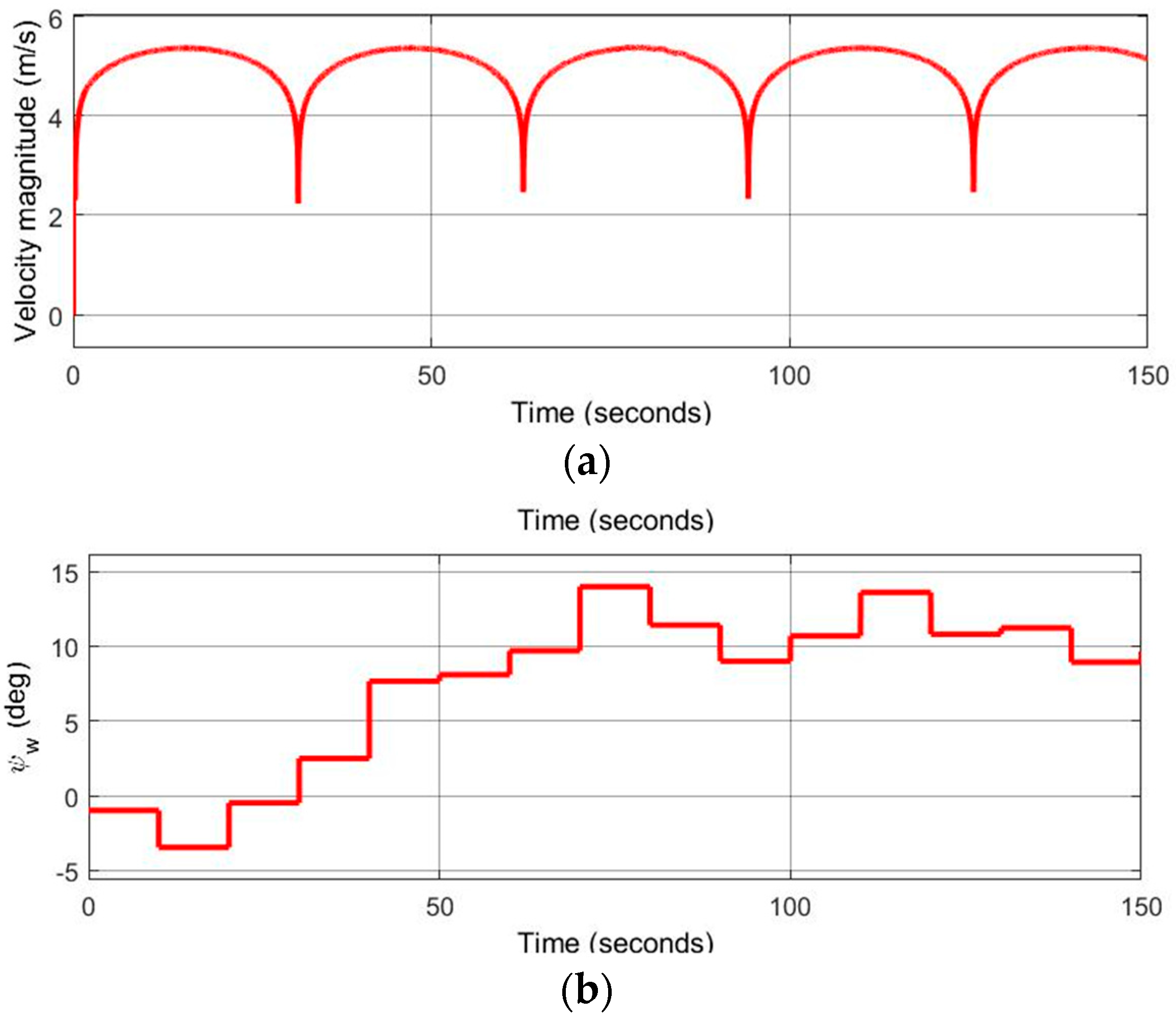
Figure 9 shows the obtained magnitude and direction (azimuth, ${\psi }_w$) of the wind affecting the UAV over time. As shown in Figure 9a, the wind velocity has points where the wind declines (to a value of $2.1\mathrm{m}/{\mathrm{s}}^2$), after which it gradually increases to a max value of $5\mathrm{m}/{\mathrm{s}}^2$. In turn, the direction of the wind (Figure 9b) changes at discrete intervals. Figure 10a,b shows the wind forces in the $x$ and $y$ directions, respectively. Figure 11 and Figure 12 provide the position and attitude responses of the UAV to the wind disturbances while trying to track the desired trajectory (Equation (43)).

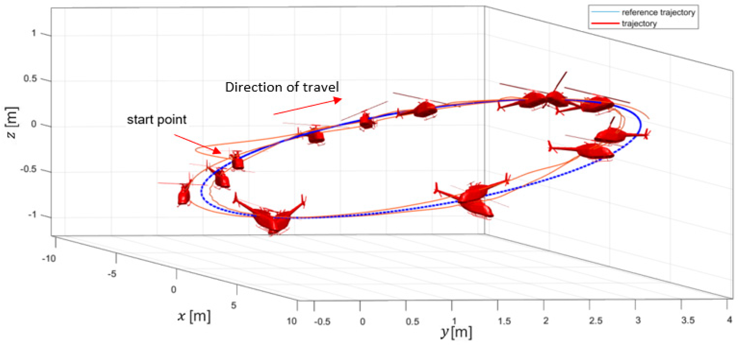
Figure 13 shows the desired and reached trajectories under variable wind disturbances. The result shows the effectiveness of the developed controller in being able to perform this maneuver, and the root mean square errors (RMSEs) obtained under all position and attitude directions were considered to be small/acceptable, as presented in

Table 4. Root mean square errors.

${\mathbf{R}\mathbf{M}\mathbf{S}\mathbf{E}}_{\mathit{x}}$	${\mathbf{R}\mathbf{M}\mathbf{S}\mathbf{E}}_{\mathit{y}}$	${\mathbf{R}\mathbf{M}\mathbf{S}\mathbf{E}}_{\mathit{z}}$	${\mathbf{R}\mathbf{M}\mathbf{S}\mathbf{E}}_{\mathit{\theta }}$	${\mathbf{R}\mathbf{M}\mathbf{S}\mathbf{E}}_{\mathit{\psi }}$
0.0281	0.1913	0.0062	0.0082	0.0082

.

From Figure 11, Figure 12 and Figure 13, it is observed that the controller was able to guide the UAV with high accuracy (i.e., the max error in translation was the same as the result for the simulation with no disturbances, Figure 5). However, this UAV had experienced some challenges managing the coupled lateral and roll motions as it flew (although such deviations were small).

6. Conclusions

The proposed nonlinear trajectory controller is based on the INDI controller technique, which includes an outer NDI/INDI loop controller for position and an inner INDI loop controller for attitude. The controllers are used in combination with PD/PID controllers to provide appropriate control inputs for the NDI/INDI blocks. The linear controllers’ gains are tuned manually and show satisfying results for different flight maneuvers. In order to improve the disturbance rejection capability of the NDI controller in the $y$ channel, a single-layer sigma-pi neural network is added, and the simulation result demonstrates its ability to compensate for the control law. Finally, several simulations demonstrate the ability of the controller to follow different trajectories under moderate external disturbances (wind gusts).

7. Future Work

In this paper, the pitch angles of the propeller are considered constant; that is, the variable pitch capabilities of the aircraft are not utilized. However, in order to take advantage of the full capacity of the designed UAV, investigating the relation between the blade pitch angle and the aerodynamic coefficient will be performed in future work. Furthermore, work will be conducted in enhancing the developed controller to include the necessary control allocation mechanisms to compute the required configuration of the UAV in each time step. Finally, performing flight tests under incremental levels of complexity within a controlled (engineered) environment, such as flying inside a wind tunnel, followed by flight tests under real-world scenarios are future work tasks that will be performed.