Two-Dimensional Geometrical Shock Dynamics for Blast Wave Propagation and Post-Shock Flow Effects

Abstract

Geometrical shock dynamics (GSD) is a model capable of efficiently predicting the position, shape, and strength of a shock wave. Compared to the traditional Euler method that solves the inviscid Euler equations, GSD is a reduced-order model derived from the method of characteristics which results in a more computationally efficient approach since it only considers the motion of the shock front instead of the entire flow field. Here, a study of post-shock flow effects in two dimensions has been performed. These post-shock flow effects become increasingly important when modeling blast wave propagation over extended times or distances, i.e., a shock front that decays in speed and that has decaying properties behind it. A comparison between the first-order complete, fully complete and point-source GSD (PGSD) models reveals the importance of preserving an intact post-shock flow term, which is truncated by the original GSD model, in predicting blast motion. Lagrangian simulations were performed for the case of interaction between two cylindrical blast waves and the results were compared to prior experimental work. The results showed an agreement in attenuation of the maximum pressure at the Mach stem, but an overestimation of the Mach stem growth at its early stage was observed using PGSD. To address this issue, another model was developed that combines the PGSD model with shock–shock approximate theory (PGSDSS), but it excessively attenuates Mach stem evolution.

1. Introduction

In general, to study shock interaction problems numerically, one can, for example, use the Navier–Stokes equations for the case of viscous flows or the Euler equations of gas dynamics if assuming inviscid flows. The results involve all flow variables within the simulation domain such that shock fronts are either captured by detecting sharp discontinuous changes in the variables if shock-capturing schemes are applied, or explicitly introduced in the solution by shock-fitting schemes. However, since the shock front usually has a large Mach number in compressive regions, a smaller time step is needed to satisfy the Courant–Friedrichs–Lewy (CFL) condition [1] to maintain numerical stability. Moreover, the thickness of the shock front is usually on a much smaller scale compared to the grid size and large gradients are always present in the neighborhood of the shock front, so for the sake of accuracy a coarse grid resolution is not an option. Though nowadays parallel computing on graphics processing units (GPUs) enables the fast implementation and solution of the Navier–Stokes and Euler equations for shock dynamics problems with refined temporal and spatial resolution, a more computationally efficient model still has its value if it can decrease the cost by a few orders of magnitude. In particular, if there is a need to quickly run through a large number of shock dynamics cases to find an optimal configuration of, e.g., number of shocks, their individual geometry, placement, and timing relative each other, a reduced-order computational model may be preferred. This need motivated the work described herein.

For the purpose of modeling shock propagation problems numerically, the geometrical treatment of the shock behavior has received considerable attention over the last few decades. In 1957, Whitham [2,3,4] published a hyperbolic model that simplified the full Euler equations into descriptions of only the position, geometry, and strength of a shock by applying linearized characteristic rules. The resulting theory, called geometrical shock dynamics (GSD), successfully reduces the dimensionality of the problem by one [5,6], and thus the complexity, as well as the cost, of the numerical computation are significantly reduced. In GSD theory, a shock front is discretized into numerous elements, and rays are introduced as orthogonal trajectories of the successive positions of these shock front elements. Then, each element propagating along its own ray is treated as a problem of shock propagation in a non-uniform tube with solid walls. GSD allows the determination of a relation between the ray tube area and the shock Mach number—the “area–Mach number (A-M)” relation, which is the fundamental component of GSD. Notably, the same relation was independently derived by Chester [7] and Chisnell [8], separately. The results of GSD are accurate for shock propagation in uniform media with moderate shock strength if no large gradient exists in the post-shock flow. Various efforts have been made to extend the application of GSD, including modifications to accommodate for moving media [9], post-shock flow effects [10,11,12,13], and detonation waves [14,15].

2. Numerical Methods

Since only a limited number of shock dynamics problems can be solved analytically using GSD, many numerical algorithms have been developed to implement GSD models including front tracking methods [6,10,11,12,16,17,18,19,20], finite difference [5] and finite volume schemes [21,22] based on the conservation form of GSD, and a recent level-set fast marching approach [23]. Among these schemes, the front-tracking-based Lagrangian schemes appear to be the most popular ones that have been used for a wide range of shock dynamics problems, since accuracy and speed can be well balanced. First developed in two dimensions by Henshaw et al. [16] and then extended to three dimensions by Schwendeman [17], the front tracking methods use particles to represent a smooth shock front. These particles advance along individual rays normal to the shock front subjected to the local Mach number. Following this concept, Schwendeman [19] computed the propagation of shock waves in gases with non-uniform properties. Best [11] and Peace et al. [12] applied the front tracking method to quantitatively investigate the influence of the post-shock flow effect on the accuracy of GSD by taking into consideration the interaction between the shock front and the non-uniform flow behind. Qiu and Eliasson [10,18] used this approach to study the blast interaction to take advantage of its speed and achieved a good agreement with results from simulating the Euler equations. Ridoux et al. [20] extended Henshaw’s Lagrangian scheme to remove its limitation for expanding shocks.

In general, a front-tracking GSD model consists of two parts: a kinematic equation derived purely from geometry and a kinetic equation describing the shock’s motion. If $\mathit{x}$ is used to denote the position vector of a particle on the shock front, then the shock front kinematics is given by

$$\begin{array}{c}\frac{d\mathit{x}}{dt}=a_{0}M\mathit{n},\end{array}$$

(1)

where $a_0$ is the speed of sound in the undisturbed region ahead of the shock wave. The shock Mach number, M, is defined as the ratio of the shock velocity in laboratory coordinates, U, to the velocity of sound in the undisturbed gas, i.e., $M=U/a_0$, and $\mathit{n}$ refers to the unit normal to the shock front that defines the propagation direction of the particle.

One widely used kinetic equation is

$$\begin{array}{c}\frac{dM}{dt}=\frac{-a_{0}M}{g\left(M\right)}\frac{A^{\prime }}{A},\end{array}$$

(2)

where $A^{\prime }=\frac{dA}{dn}$, and $g\left(M\right)$ is given by

$$\begin{array}{c}g\left(M\right)=\frac{M}{M^2-1}\left(1+\frac{2}{\gamma +1}\frac{1-{\mu }^2}{\mu }\right)\left(1+2\mu +\frac{1}{M^2}\right),\mathrm{and}\end{array}$$

(3)

$$\begin{array}{c}{\mu }^2=\frac{(\gamma -1)M^2+2}{2\gamma M^2-(\gamma -1)},\end{array}$$

(4)

where $\gamma$ is the heat capacity ratio.

For general M, the solution of Equation (2) leads to the classic A-M relation that explicitly states how the shock front strength varies with the area upon it:

$$\begin{array}{c}\frac{A}{A_0}=\frac{f\left(M\right)}{f\left(M_0\right)},\end{array}$$

(5)

leading to

$$\begin{array}{c}f\left(M\right)=exp\{-\int g(M\left)dM\right\}.\end{array}$$

(6)

To integrate the original GSD model consisting of Equations (1) and (2), an explicit expression for $\frac{A^{\prime }}{A}=\frac{1}{A}\frac{dA}{dn}$ is needed. In fact, $A^{\prime }/A$ is the curvature of the shock front, $\kappa$. The proof starts from one assumption of GSD theory, that the rays are normal to the surface, which leads to

$$\begin{array}{c}\nabla ·\frac{\mathit{n}}{A}=0.\end{array}$$

(7)

This can be rewritten as

$$\begin{array}{c}\nabla ·\mathit{n}-\frac{\mathit{n}·\nabla A}{A}=0.\end{array}$$

(8)

Finally,

$$\begin{array}{c}\frac{\mathit{n}·\nabla A}{A}=\frac{1}{A}\frac{dA}{dn}=\frac{A^{\prime }}{A}\Rightarrow \frac{A^{\prime }}{A}=\nabla ·\mathit{n}=\kappa .\end{array}$$

(9)

Therefore, the A-M relation can now be replaced by the $\kappa$-M relation.

The $\kappa$-M relation represents the rate of change in the shock front Mach number subject to the local curvature, so it can be numerically integrated. Moreover, given that it is always cumbersome to define ray tubes and compute the cross-section areas in the original GSD method, another advantage of replacing the A-M relation with the $\kappa$-M relation is that, unlike ray tubes that only exist virtually, curvature is clearly defined in differential geometry.

All quantities required for Equations (1) and (2) are thus known. The two-dimensional GSD model now can be numerically solved at a set of particle locations ${\mathit{x}}_{\mathit{i}}$. The discretized forms of the ordinary differential equations become

$$\begin{array}{c}\frac{d{\mathit{x}}_i}{dt}=a_0{M}_i{\mathit{n}}_i,\end{array}$$

(10)

$$\begin{array}{c}\frac{d{M}_i}{dt}=\frac{-a_0{M}_i}{g\left(M_i\right)}{\kappa }_i,\end{array}$$

(11)

for $i=1,2,\dots N$, and should be integrated simultaneously. This can be achieved by, for example, adopting a third-order Runge–Kutta scheme [24]. In this work, the third-order Runge–Kutta scheme was selected over a fourth-order one because it achieved similarly accurate results given the spatial resolution, with fewer evaluations per time step.

For the purpose of evaluating the curvature, spline interpolation can be fitted to the shock front with the parameterization with respect to arc length. If $s_i$ is used to denote the arc length along the curve from the first particle to particle i, it can be approximated as shown below with satisfying precision, assuming that the particle density is sufficient.

$$s_i\left(t\right)=\left\{\begin{array}{cc}0\hfill & \mathrm{if}i=1,\hfill \\ s_{i-1}\left(t\right)+{\parallel {\mathit{x}}_i\left(t\right)-{\mathit{x}}_{i-1}\left(t\right)\parallel }_2\hfill & \mathrm{if}i=2,3,\dots N.\hfill \end{array}\right.$$

(12)

Then, the first- and second-order derivatives required for curvature can be obtained at particles from spline interpolation. An approximation of the arc length is necessary, which requires the shock front to be adequately resolved. Guided by the resolution conditions proposed by Henshaw et al. [16], an appropriate number of particles that balances accuracy and speed should be selected to represent the shock front. If the average arc length between particles is denoted by $d{s}_{\mathrm{avg}}$, the criterion is given by

$$\begin{array}{c}\Delta s_{\mathrm{avg}}\left(0\right)=\frac{s_N\left(0\right)}{N}=k_1\ll 1.\end{array}$$

(13)

This condition provides a lower bound on the number of particles, and typically $k_1$ is set to 0.01. To maintain shock front resolution throughout the Lagrangian simulation, a scheme that adds or deletes particles according to the local density is needed, because particles tend to spread out in expanding regions and cluster in compressive regions. Here, the particle spacing is checked every few time steps using

$$\begin{array}{c}{\sigma }_{\min }\le {\sigma }_i\left(t\right)=\frac{\Delta s_i\left(t\right)}{\Delta s_{\mathrm{avg}}\left(t\right)}\le {\sigma }_{\max }\mathrm{for}i=2,3,...N,\end{array}$$

(14)

where $\Delta s_i\left(t\right)=s_i\left(t\right)-s_{i-1}\left(t\right)$, and ${\sigma }_{\min }$ and ${\sigma }_{\max }$ are typically set to be 0.5 and 1.5, respectively. If ${\sigma }_i\left(t\right)>{\sigma }_{\max }$, a particle is added using spline interpolation evaluated at $\frac{1}{2}(s_i\left(t\right)+s_{i-1}\left(t\right))$, and if ${\sigma }_i\left(t\right)<{\sigma }_{\min }$, particle ${\mathit{x}}_i$ is deleted. Given that the accumulation of particles in compressive regions drastically restricts the time step to avoid ray crossing, by removing redundant particles, not only is the numerical cost reduced, but numerical stability is ensured at each time step.

The two-step smoothing procedure is another component of the numerical implementation of GSD that is used to dampen high frequency errors in ${\mathit{x}}_i\left(t\right)$ and $M_i\left(t\right)$. If ${\tilde{\mathit{x}}}_i$ and ${\tilde{M}}_i\left(t\right)$ denote the smoothed position and Mach number associated with the ith particle, respectively, then the smoothing procedure is given by

$$\begin{array}{c}{\tilde{\mathit{x}}}_i\left(t\right)=\frac{1}{2}\left({\mathit{x}}_{i-1}\left(t\right)+{\mathit{x}}_{i+1}\left(t\right)\right),\end{array}$$

(15)

$$\begin{array}{c}{\tilde{M}}_i\left(t\right)=\frac{1}{2}\left(M_{i-1}\left(t\right)+M_{i+1}\left(t\right)\right),\end{array}$$

(16)

where first i-even and then i-odd particles are scanned. Best [11] found it desirable to apply such a smoothing procedure for compressive flows every few time steps, but that is unnecessary in the case of expanding flows.

An appropriate time step size is guided by the CFL condition. Following Henshaw’s work [16], the scheme used in this study that provides the upper bound on the selection of a time step, $\Delta t$, is given by

$$\begin{array}{c}\frac{\Delta t}{\Delta s_{\min }\left(t\right)}=\frac{\Delta t}{{\sigma }_{\min }\Delta s_{\mathrm{avg}}}<k_2,\end{array}$$

(17)

where the constant $k_2$ is usually taken to be 0.2.

3. Application of GSD to an Expanding Blast Wave

It is well known that GSD is accurate for shock waves with constant properties behind the shock front [4,5,10,13,16]. For a blast wave, the flow properties behind the shock front are decaying exponentially. This contradicts the assumption made in deriving GSD, which requires a uniform state behind the shock. To investigate whether the accuracy is compromised if this assumption is violated, we start by comparing Whitham’s original GSD model with Bach and Lee’s analytical solution [25] and the simulation using the Euler equations. The latter two solutions not only provide initial conditions for the Lagrangian schemes but also are used as a reference to evaluate the accuracy of GSD models in predicting blast motion.

3.1. Original GSD Model

Whitham’s original GSD model, in its discretized form (Equations (10) and (11)), was solved first. To start the original GSD scheme, a shock front was represented by particles placed on a circle with a radius of 10 mm with spacing $\Delta s\approx 0.1$ mm. The corresponding Mach number at $R_0=10$ mm was found to be 11.81, via a simulation of the Euler equations, and 9.76 from the analytical solution. Smoothing procedures are not needed for a single blast expansion but particles are added if the local particle density becomes sparse as the blast front area increases.

To solve the Euler equations, we use the open-source framework called Overture [26], which has been introduced and validated in detail prior to this study [27,28,29]. To simulate blast propagation in air, the conservation laws of mass, momentum, and energy for inviscid compressible flows are solved with a second-order Godunov scheme [30]. Instead of simulating a condensed energy source, the solver is initialized with a specific wave front of finite size such that the requirement of a fine mesh and numerical oscillations arising from sharp discontinuities at the wave front can be avoided. The initial conditions used for the Euler equations are based on Taylor’s similarity law [31], outlined in Appendix B. For two-dimensional blast dynamics problems, Taylor’s similarity law can be modified to generate initial conditions for cylindrical blasts [32]. Details of the verification of the Euler solver, a description of the initial conditions, the computational domain set-up, and a grid independence study are presented in Appendix A.

Both Bach and Lee’s analytical solution and the Euler equations for a single cylindrical point-blast were numerically solved with an initial energy of $E_0=8000$ J/m. To study the shock front behavior during its expansion, the variation in Mach number as a function of radius (i.e., M-R) is shown in Figure 1. A discrepancy can be observed between the M-R curves from the analytical and Euler solutions at an early stage when the blast front is very strong. The two curves gradually become closer as the blast front further expands and almost agree once the radius exceeds its initial size by a factor of 20.

The GSD results are presented in Figure 1, where each resulting M-R curve lies well above its corresponding reference. This indicates that the blast front was not sufficiently attenuated throughout the Lagrangian simulation by the original GSD model. This result shows the importance of including the post-shock flow effect into the GSD model.

3.2. First-Order Complete GSD Model

To explore the reason why GSD is less accurate when applied to blast waves, the derivation of Whitham’s original model needs to be re-evaluated without linearizing conservation equations about the local conditions. One important derivation is through the characteristic form of its solution. The compatibility equation along the $C_{+}$ characteristics is

$$\begin{array}{c}\frac{\partial p}{\partial t}+(u+a)\frac{\partial p}{\partial x}+\left(\rho a\right)\left(\frac{\partial u}{\partial t}+(u+a)\frac{\partial u}{\partial x}\right)+\rho u{a}^2\frac{A^{\prime }\left(x\right)}{A\left(x\right)}=0,\end{array}$$

(18)

with p, u, a, and $\rho$ denoting pressure, particle velocity, speed of sound, and density of the flow, respectively.

By relating ${\partial }_{t}p$, ${\partial }_{x}p$ to $d_{t}p$ and ${\partial }_{t}u$, ${\partial }_{x}u$ to $d_{t}u$ along the shock trajectory, a simple manipulation yields

$$\begin{array}{c}\left(\frac{dp}{dM}+\rho a\frac{du}{dM}\right)\frac{dM}{dt}=-\left[a_{0}M\frac{\rho u{a}^2}{u+a}\frac{A^{\prime }\left(x\right)}{A}+\underset{\mathrm{Term}\mathrm{A}}{\underbrace{\left(\frac{a_{0}M}{u+a}-1\right)\left(\frac{\partial p}{\partial t}+\rho a\frac{\partial u}{\partial t}\right)}}\right].\end{array}$$

(19)

The equivalence of Equation (19) to Equation (2) is established by the use of shock jump conditions in the determination of $dp/dM$ and $du/dM$, along with the truncation of “term A” in Equation (19). Best [11] concluded that the criterion of Whitham’s A-M relation being a good approximation through linearization is

$$\begin{array}{c}{a}_{0}M\frac{\rho u{a}^2}{u+a}\left|\frac{A^{\prime }\left(x\right)}{A}\right|\gg |\frac{a_{0}M}{u+a}-1|\underset{\mathrm{Post}-\mathrm{shock}\mathrm{flow}\mathrm{term}}{\underbrace{|\frac{\partial p}{\partial t}+\rho a\frac{\partial u}{\partial t}|}}.\end{array}$$

(20)

Equation (20) lists two sources of disturbances that possibly modify the shock front: (1) the term on the left-hand side of the inequality characterizes the effect of changing area upon the shock front, and (2) the right-hand side represents the interaction between the shock front and the flow behind it. The post-shock flow term describes the non-uniformity of the flow behind the shock. This term is equal to zero for a uniform flow, which is exactly the case of applying small perturbation theory to deduce the A-M relation, as performed by Whitham. Even though the change in area upon the shock front disturbs the flow immediately behind it such that the post-shock flow term is bigger than zero, its absolute value is usually very small along the $C_{+}$ characteristics originating from a uniform state. This justifies the appropriateness of using the A-M relation to describe the motion of an initially uniform shock wave. However, this term can also be fairly large if a strong gradient exists in the flow just behind the shock front. To what extent such a non-uniformity affects the shock motion is determined by $|\frac{a_{0}M}{u+a}-1|$, which indicates the coincidence of the $C_{+}$ characteristic line and the shock trajectory. Recall that when deriving the A-M relation, the compatibility equation along the $C_{+}$ characteristics is applied at the shock front by using the shock jump conditions, but such being a good approximation requires the leading $C_{+}$ characteristic to coincide with the shock trajectory. This is true only in the sonic limit, i.e., $M\to 1$, where the disturbances stemming from the non-uniform flow behind the shock propagate along the $C_{+}$ characteristics but do not meet the shock front and, therefore, they impose no influence on its motion. On the other hand, if $M\to \infty$, Best reported that $|\frac{a_{0}M}{u+a}-1|$ tends to be 0.215 for $\gamma =1.4$ [11], which suggests the significance of the post-shock flow effect, as in this situation disturbances overtake and then modify the shock front. Consequently, since the right-hand side of Equation (20) is non-zero for most cases, the A-M relation is accurate only when the effect of area change upon the shock dominates that of the interaction between the shock front and the non-uniform flow behind it.

For the case of shocks with decaying properties behind, blast waves for example, the gradient in the flow immediately behind the shock front can make the post-shock flow term very large. As long as the shock is of moderate strength, disturbances will catch up with the shock front and modify it. The inequality in criterion (20) is then violated, since the right-hand side becomes as significant as the left-hand side in terms of magnitude. Therefore, to make the A-M relation appropriate for this type of shock dynamics situation, a correction term must be added that accounts for the post-shock flow effect, and obviously, the truncated term itself is a good starting point. A generalization of GSD was carried out by Best [11], who closed the motion rule for shock propagation by an infinite sequence of ordinary differential equations given as follows

$$\begin{array}{c}\frac{dM}{dt}=\frac{-a_{0}M}{d_{M}p+\rho a{d}_{M}u}\left[\left(\frac{\rho u{a}^2}{u+a}\right)\frac{A^{\prime }}{A}+\left(\frac{1}{u+a}-\frac{1}{a_{0}M}\right)Q_1\right],\end{array}$$

(21)

$$\begin{array}{c}\begin{array}{cc}\hfill \frac{d{Q}_k}{dt}=& -a_{0}M\{\frac{{\partial }^k}{\partial t}\left(\frac{\rho u{a}^2}{u+a}\right)\frac{A^{\prime }}{A}+\sum _{i=1}^k\left[\left(\genfrac{}{}{0pt}{}{k}{i}\right)\frac{{\partial }^i}{\partial t}\left(\frac{1}{u+a}\right)Q_{k-i+1}\right]\hfill \\ & +\frac{{\partial }^{k-1}}{\partial t}\left(\frac{\partial \left(\rho a\right)}{\partial t}\frac{\partial u}{\partial x}-\frac{\partial \left(\rho a\right)}{\partial x}\frac{\partial u}{\partial t}\right)+\left(\frac{1}{u+a}-\frac{1}{a_{0}M}\right)Q_{k+1}\},\hfill \end{array}\end{array}$$

(22)

for $k=1,2,\dots$, where

$$\begin{array}{c}{Q}_k=\frac{{\partial }^{k-1}}{\partial t}\left(\frac{\partial p}{\partial t}+\rho a\frac{\partial u}{\partial t}\right).\end{array}$$

(23)

The above closed system can be written in a concise form by setting M to be $Q_0$: $d_t{Q}_k=f(Q_0,\dots ,Q_{k+1},A^{\prime }/A)$, for $k=0,1,\dots$. Evidently the expression for $d_t{Q}_k$ depends on $Q_{k+1}$, such that each differential equation in the system is coupled to its successor in the sequence. By truncating all the terms involving $Q_{k+1}$, a kth-order complete GSD system is achieved. It is so named because there remain no derivatives of orders higher than k, leading to the post-shock flow effect being partially complete. For example, the front-tracking-based two-dimensional original GSD model consisting of Equations (1) and (2) only achieves zeroth-order completeness. Moreover, if $Q_1$ is preserved but terms involving $Q_2$ are discarded, the first-order complete GSD model is obtained as follows, which contains three coupled ordinary differential equations for three unknowns, namely, $\mathit{x}\left(t\right)$, $M\left(t\right)$, and $Q_1\left(t\right)$:

$$\begin{array}{c}\frac{d\mathit{x}}{dt}=a_{0}M\mathit{n},\end{array}$$

(24)

$$\begin{array}{c}\frac{dM}{dt}=\frac{-a_{0}M}{d_{M}p+\rho a{d}_{M}u}\left[\left(\frac{\rho u{a}^2}{u+a}\right)\frac{A^{\prime }}{A}+\left(\frac{1}{u+a}-\frac{1}{a_{0}M}\right)Q_1\right],\end{array}$$

(25)

$$\begin{array}{c}\frac{d{Q}_1}{dt}=-a_{0}M\left[\frac{\partial }{\partial t}\left(\frac{\rho u{a}^2}{u+a}\right)\frac{A^{\prime }}{A}+\frac{\partial \left(\rho a\right)}{\partial t}\frac{\partial u}{\partial x}-\frac{\partial \left(\rho a\right)}{\partial x}\frac{\partial u}{\partial t}+\frac{\partial }{\partial t}\left(\frac{1}{u+a}\right)Q_1\right].\end{array}$$

(26)

Once initial conditions are provided, the system can then be solved by numerical integration.

In this study, the first-order complete GSD model was solved with the Lagrangian scheme for the same case as the original GSD model presented in Section 2. In addition to the initial blast radius and Mach number, the initial value of $Q_1$ is also necessary. Since $Q_1$ requires partial derivatives with respect to time and location, which are not present until the scheme advances at least one time step, it is only possible to estimate its value at $R_0=10$ mm using some prior knowledge. By estimating $d_{x}M$ from the analytical solution, all partial derivatives can be computed as functions of $d_{x}M$ [11] and then $Q_1$ follows.

3.3. Modified GSD Model

To investigate if solving a higher-order complete GSD model leads to a better accuracy, Equation (19) is revisited. By explicitly computing the post-shock flow term, ${\partial }_{t}p+\rho a{\partial }_{t}u$, through the similitude relation $d_{x}M\left(M\right)$ obtained from the analytical solution, the so-called modified GSD model [10] is obtained as follows

$$\begin{array}{c}\frac{d\mathit{x}}{dt}=a_{0}M\mathit{n},\end{array}$$

(27)

$$\begin{array}{c}\frac{dM}{dt}=\frac{-a_{0}M}{d_{M}p+\rho a{d}_{M}u}[\underset{\mathrm{Geometrical}\mathrm{effect}}{\underbrace{\left(\frac{\rho u{a}^2}{u+a}\right)\frac{A^{\prime }}{A}}}+\underset{\mathrm{Post}-\mathrm{shock}\mathrm{flow}\mathrm{effect}}{\underbrace{(\frac{1}{u+a}-\frac{1}{a_{0}M})(\frac{\partial p}{\partial t}+\rho a\frac{\partial u}{\partial t})}}].\end{array}$$

(28)

This model preserves the full solution without truncation at any level of $Q_k$.

3.4. Point-Source GSD Model

The analytical solution to point-blast propagation and an improved GSD model, point-source GSD model (PGSD), will be introduced next. Considering that Bach and Lee’s analytical solution to point-blast propagation [25], outlined in Appendix C, already describes an accurate blast behavior, a modification to the original GSD model to include this essential blast property was proposed by Yoo and Butler [33]. Using Taylor’s similarity law [31] and Equation (11) together with expressions for shock front speed, ${\dot{R}}_s=\frac{d{R}_s}{dt}=a_{0}M$, and shock front acceleration, ${\ddot{R}}_s=a_0\frac{dM}{dt}$, the following expression is obtained

$$\begin{array}{c}\frac{dM}{dt}=\frac{a_0{M}^2\theta }{R_s}=\frac{-a_{0}M}{-j/M\theta }\frac{j}{R_s},\end{array}$$

(29)

where $j=0,1,2$ for planar, cylindrical, and spherical waves. $R_s$ is the shock radius. $\theta$ is a function of M given by

$$\begin{array}{c}\theta \left(M\right)=\frac{R_s{\ddot{R}}_s}{{\dot{R}}_s^2}.\end{array}$$

(30)

In fact, $j/R_s$ is the curvature of a cylindrical ($j=1$) and spherical ($j=2$) blast front, meaning that $dM/dt$ can be further expressed as

$$\begin{array}{c}\frac{dM}{dt}=\frac{-a_{0}M}{\Phi \left(M\right)}\kappa ,\end{array}$$

(31)

where $\Phi \left(M\right)=-j/\left(M\theta \right)$.

Equation (31), which is the $\kappa$-M relation for the particular blast front, is the core of the PGSD model. The main advantage of this model is that it defines the motion rule of blast propagation for all energy contents without the need to specify $\theta \left(M\right)$ for a particular point-source explosion. Moreover, the PGSD model can be further modified for condensed explosives as long as the resulting blast behavior is known beforehand. In this situation, M-R data can be used to generate $\Phi \left(M\right)$ that encodes essential blast information for that particular charge.

3.5. Post-Shock Flow Effect

The influence of the completeness of the post-shock flow term is best illustrated as shown in Figure 2, where the values of the first term in Equation (28) times the geometrical effect term, and the post-shock flow effect term, respectively, are tracked throughout the Lagrangian simulation. Since the opposite of these two terms make up the blast acceleration, $dM/dt$, a positive value signals its effect in attenuating the blast front. On the other hand, starting at the same initial value, the post-shock flow effect from the modified GSD model soon departs from the first-order complete GSD result on its way to the peak value. Then, the curve gradually decreases and falls below its counterpart at $R\approx 17$ mm. Such an observation of the post-shock flow effects at an early stage is echoed in the M-R curves, where the modified GSD model attenuates the blast front as accurately as the analytical solution, while the first-order complete GSD model predicts a stronger blast. The post-shock flow effect estimated by the first-order complete GSD model keeps increasing until arriving at its highest point at $R\approx 25$ mm, but its variance with the modified GSD result accumulates until the two curves intersect for a second time. This explains the over-attenuation of the blast velocity further away from the explosion center by the first-order complete GSD model.

Using these four models, original GSD, first-order complete GSD, modified GSD, and PGSD, to solve for the expansion of a cylindrical blast wave in air with initial conditions $M_0=9.76$ and $R_0=10$ mm, yields the results presented in Figure 3. The geometrical effects obtained from solving the first-order complete GSD model and from the modified GSD model do not deviate much from each other, as seen in Figure 3, the change of area upon the blast front should not be the reason for the discrepancy manifested in the blast behaviors for these two models.

Obviously, the first-order complete GSD model succeeds in attenuating the blast front when compared to the original GSD model, however, the first-order complete GSD model predicts a much weaker blast at distances beyond 23 mm. The results of the modified GSD overlap with those of the PGSD model, which in turn overlap with the analytical result, as expected, since both the modified GSD and PGSD models preserve the full solution, i.e., there is no truncation of the $Q_k$ terms. Therefore, by comparing the post-shock flow effects from the two models and analyzing how their resulting blast behaviors differ, a conclusion can be made here that the level of the completeness of the post-shock flow term determines the accuracy of geometrical shock dynamics when being applied to expanding blast waves.

3.6. Interaction of Two Cylindrical Blast Waves Using PGSD

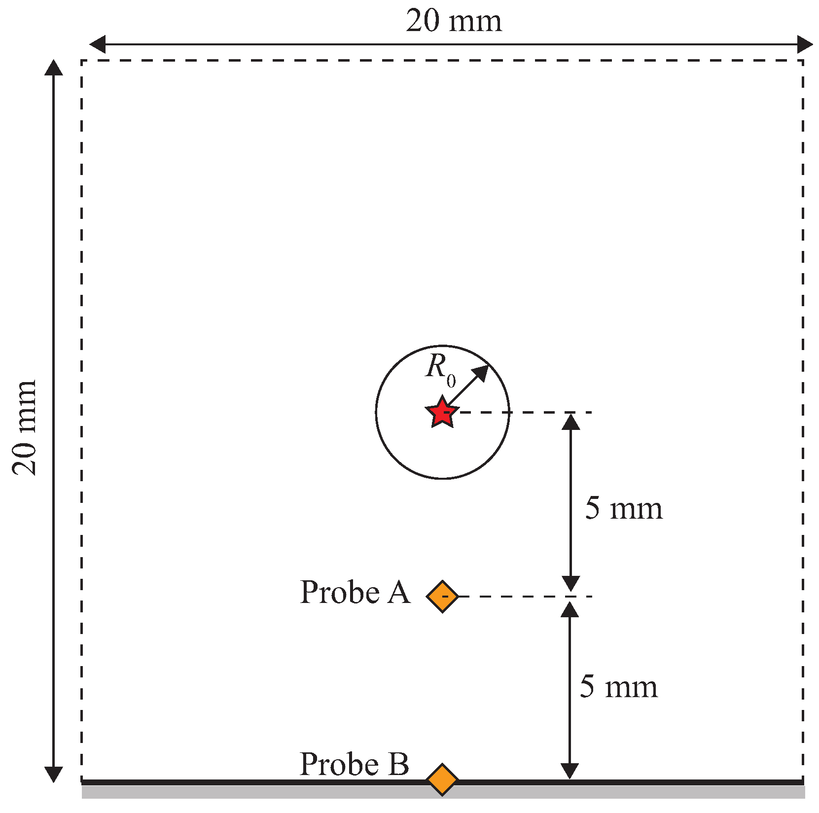
Higashino et al. [34] carried out experiments on the interaction of a pair of identical blast waves in 1991. By rapidly discharging a high voltage through two thin metal wires, the wires exploded as a result of the applied voltage and two cylindrical shock waves were generated simultaneously. The same wires, made of either copper or nichrome, were used in an experiment. Each wire was 34 mm in length and 0.1 mm in diameter. The two wires were placed side by side 60 mm apart, as shown in Figure 4. The energy from the wire explosions were estimated by Higashino to be 25 J and 170 J for the copper and nichrome wires, respectively. Later, Qiu [10] successfully replicated the experiments using energy density of 59 J/m and 117 J/m, respectively, in his simulations.

In this study, Higashino’s experiments, mentioned above, were chosen to test the PGSD model’s performance on blast interaction. First, the critical conditions for the transition from regular to irregular reflection taking place where two neighboring blasts intersect is determined. If prior knowledge is accessible, the instantaneous Mach number and position of the shock front can be obtained through processing, e.g., experimental schlieren images or data from simulations. An approach to compute the transition conditions from regular to irregular reflection for the interaction between two identical cylindrical shocks was introduced by [10] by communicating the shock motion known beforehand to the sonic criterion [35] via the wedge angle (defined in Figure 4). Following this approach, the initial conditions for the copper and nichrome wires in the current PGSD simulations were determined to be $M_0=1.13,r_0=46.60$ mm and $M_0=1.30,r_0=41.46$ mm, respectively. These initial conditions will be referred to as I.C.1. The initial two-blast front was discretized with five particles per degree, i.e., $\Delta s\approx 0.2$ mm for the copper and $\Delta s\approx 0.18$ mm for the nichrome wire case. A second set of initial conditions, based on von Neumann’s detachment theory [36], was also used. These initial conditions are referred to as I.C.2. and were determined to be $M_0=1.25,r_0=42.83$ mm and $M_0=1.50,r_0=45.96$ mm for the copper and nichrome wires, respectively.

To replicate the experiment, the multi-blast front, that is considered as a continuous curve in two-dimensional space, is represented by particles. Given that a perfect circular shape is well preserved before any Mach stem arises, it is rational to assume that the velocity is evenly distributed along the shock front. Given the initial conditions, the Mach number and coordinate are stored for each particle. Then, the PGSD model was solved using the Lagrangian scheme with mesh smoothing and regularization procedures applied dynamically based on the shock front configuration and particle resolution. It should be noted that time steps start counting at the regular to irregular transition instant.

The time history of the maximum pressure at the Mach stem was recorded in the PGSD Lagrangian scheme and compared to the modified GSD results, as shown in Figure 5. The results shown in Figure 5 suggest that the two models’ solutions to the same explosion case agree in trend but differ in pressure values at the same time instance. The maximum pressure curves from the PGSD model always lie above the modified GSD results for both cases. Such a discrepancy may come from differences in the definition of the reference time, i.e., the transition time instant, or from distinct intrinsic properties of the two models in terms of how the post-shock flow effect is dealt with.

The transition conditions measured in the experiments by Higashino et al. contain some uncertainties simply due to the temporal and spatial resolutions of the experimental equipment and details of the published data. Therefore, the second set of initial conditions, I.C.2, were used, and these resulted in a better match of the PGSD model to the experimental data, as shown in Figure 6.

By matching the arrival time of the undisturbed part of the shock front in a least squares sense, as illustrated in Figure 6, the timeline of the Lagrangian simulation is consistent with that of the corresponding experiment. This makes the time history of the maximum pressure at the Mach front from the PGSD model comparable to the experimental data.

Figure 7 summarizes the difference in results from the PGSD scheme using the two different sets of initial conditions, which also shows the challenge of choosing the correct initial conditions. The most noticeable difference to the experimental data is that the PGSD’s pressure value is higher than its counterpart at the same time instance for each case of initial conditions. This means that a faster Mach stem is predicted by the PGSD model, which is in agreement with earlier observations [10,13]. Considering that GSD tends to generate irregular reflection in compressive flows even when regular reflection is supposed to occur, the overestimation of Mach stem growth seems to be inevitable.

4. Modifying PGSD Using Shock–Shock Approximate Theory

Whitham [4] applied shock–shock approximate theory to the diffraction of a planar shock by a straight wedge [4], as illustrated in Figure 9, and achieved a triple-point trajectory close to that observed in experiment. Schwendeman [37] extended this approach to investigate the evolution of Mach reflection arising from the convergence of shocks. As a result, an original polygonal shape repeats itself at successive intervals and Mach numbers increase in agreement with the analytical solution. Inspired by these works, a new GSD model was developed in this study aiming at overcoming GSD’s tendency of producing irregular reflection in compressive regions even though a regular reflection is expected. This model is referred to as the point-source GSD model with shock–shock approximate theory (PGSDSS).

4.1. Shock–Shock Approximate Theory for Planar Shock Diffraction by a Wedge

When a Mach stem has already been formed, the shock front is separated by the triple point into two regions in which the Mach number is constant: $M_0$ for the undisturbed part and $M_w$ for the Mach stem (see Figure 8). The angle $\chi$ is the deflection angle measured between the triple-point trajectory and the wedge surface tilted at ${\theta }_w$ above the horizontal ground. If a straight Mach stem is assumed, the undisturbed rays contained in a stream tube of area $A_0=\overline{A{B}^{\prime }}sin(\chi +{\theta }_w)$ pass through the area $A_w=\overline{A{B}^{\prime }}sin\left(\chi \right)$, so a relationship can be obtained by using the A-M relation (5) to correlate ray tube area and Mach number

$$\begin{array}{c}\frac{f\left(M_w\right)}{f\left(M_0\right)}=\frac{sin\left(\chi \right)}{sin(\chi +{\theta }_w)},\end{array}$$

(32)

Since the shock front is continuous at the triple point, the distance traveled by the triple point as part of the undisturbed shock should be the same as that being the lower part of the Mach stem, i.e., $\overline{A{B}^{\prime }}=a_0{M}_{0}t/cos(\chi +{\theta }_w)=a_0{M}_{w}t/cos\left(\chi \right)$, resulting in

$$\begin{array}{c}\frac{M_w}{M_0}=\frac{cos\left(\chi \right)}{cos(\chi +{\theta }_w)}.\end{array}$$

(33)

Given the Mach number of the planar incident shock, $M_0$, and wedge angle, ${\theta }_w$, Equations (32) and (33) provide solutions to $\chi$ and $M_w$. In this shock–shock approximate theory, nothing more than the trajectory of the triple point is yielded, which is described by the single variable $\chi$.

4.2. Shock–Shock Approximate Theory for Cylindrical Shock Diffraction by a Wedge with Continuously Decreasing Tilt Angle

Then, we take one step further to consider the interaction between two identical cylindrical shocks. This is equivalent to the diffraction of a cylindrical shock by a straight wedge with continuously decreasing tilt. One difficulty is how to extend the theory developed for a planar shock to a curved one. The most straightforward way is to simply treat the incident shock as a planar shock in the three-shock configuration, as indicated in Figure 9. Once the transition angle ${\theta }_{wc}$ is reached, the Mach stem forms from the wedge surface, presumably in a perpendicular manner. Then, solve Equations (32) and (33), with ${\theta }_w$ being the instantaneous wedge angle and $M_0$ being the Mach number for the expanding cylindrical shock. The resulting deflection angle, $\chi$, and Mach number at the wall, $M_w$, together give the location of the triple point after an infinitesimal period of time $\Delta t$, i.e., $B^{\prime }=(x_A+M_w{a}_0\Delta t,y_A+tan\left(\chi \right)M_w{a}_0\Delta t)$. However, $B^{\prime }$ is not guaranteed to be on the undisturbed part of the shock front as there is no constraint on the radial position of the triple point in Equations (32) and (33).

In contrast, the circular geometry of the undisturbed part of the shock front is communicated to the triple point in an improved theory, as illustrated in Figure 10. Here, A is still the current location of the triple point but the cylindrical incident shock is no longer simplified as a planar shock. Instead, a curved shock element is considered as the incident shock in the three-shock configuration and its curved shape is preserved in developing the theory, except when computing its ray area. This makes sense because in the Lagrangian scheme the arc length between two neighboring particles is approximated as a straight line in the calculation of the A-M relation. The other end of the cylindrical shock element, point B, will become the triple point located at $B^{\prime }$ after an infinitesimal time interval, but its current position is unknown. As a result, the instantaneous wedge angle, ${\theta }_w$, is unknown, considering that in the original shock–shock approximate theory the wedge bottom surface is always parallel to the propagation direction of the incident shock that nonetheless depends on the choice of B. In fact, ${\theta }_w$ is related to the location of B as follows:

$$\begin{array}{cc}\hfill \angle A^{\prime }A{A}^{″}+\angle B^{\prime }A{A}^{\prime }+\angle BA{B}^{\prime }+\angle OAB& =\pi ,\hfill \\ \hfill ⟶\angle A^{\prime }A{A}^{″}+\chi +\frac{\pi }{2}-\chi -{\theta }_w+\frac{\pi -{\theta }_c}{2}& =\pi ,\hfill \\ \hfill ⟶{\theta }_w& =\angle A^{\prime }A{A}^{″}-\frac{{\theta }_c}{2},\hfill \end{array}$$

where point O is the explosion center that is given in the initial conditions, and ${\theta }_c$ is the central angle of the minor arc between points A and B.

Similar to the shock–shock approximate theory for plane shock diffraction by a wedge, the relationship between Mach numbers $M_w$ and $M_0$ is established by $M_w/M_0=\overline{A{A}^{\prime }}/\overline{B{B}^{\prime }}$. The law of sines further gives

$$\begin{array}{c}\frac{\overline{A{A}^{\prime }}}{\overline{B{B}^{\prime }}}=\frac{\overline{A{A}^{\prime }}/\overline{A{B}^{\prime }}}{\overline{B{B}^{\prime }}/\overline{A{B}^{\prime }}}=\frac{cos\left(\chi \right)}{sin(\frac{\pi }{2}-{\theta }_w-\chi )/sin(\frac{\pi }{2}+\frac{{\theta }_c}{2})}\end{array}$$

(34)

yielding

$$\begin{array}{c}\frac{M_w}{M_0}=\frac{cos\left(\chi \right)cos\left(\frac{{\theta }_c}{2}\right)}{cos(\chi +{\theta }_w)}.\end{array}$$

(35)

On the other hand, the undisturbed rays contained in a stream tube of area $A_0=\overline{AB}$ passing through the area $A_w=\overline{A^{\prime }{B}^{\prime }}$ lead to

$$\begin{array}{c}\frac{f\left(M_w\right)}{f\left(M_0\right)}=\frac{sin\left(\chi \right)sin(\frac{\pi }{2}+\frac{{\theta }_c}{2})}{sin(\chi +{\theta }_w-\frac{{\theta }_c}{2})}.\end{array}$$

(36)

The last component is a constraint that enforces the radial position of point $B^{\prime }$ to be on the undisturbed part of the shock front after an infinitesimal time span. This leads to another advantage of using a cylindrical shock as the incident shock over the simplification into a planar shock. The constraint is given by

$$\begin{array}{c}\parallel (x_A+M_w{a}_0\Delta t,y_A+tan\left(\chi \right)M_w{a}_0\Delta t)-(x_O,y_O)\parallel =\overline{O{B}^{\prime }},\end{array}$$

(37)

which completes the shock–shock approximate theory for cylindrical diffraction off a wedge with continuously decreasing tilt angle.

4.3. Point-Source GSD Model with the Shock–Shock Approximate Theory

A system comprising Equations (35)–(37) along with the relation ${\theta }_w=\angle A^{\prime }A{A}^{″}-{\theta }_c/2$ can now be solved by a numerical algorithm, with $x_A$, $y_A$, ${\theta }_w$, and $M_0$ known at the current time step. The radius of the undisturbed part of the shock front at the next time step, $\overline{O{B}^{\prime }}$, is not necessary to be determined at point $B^{\prime }$ that is yet unknown; instead, the average radius can be used, which is known after integrating the PGSD model for a time interval $\Delta t$. The triple point is always part of the undisturbed shock front, whose propagation is well described by the PGSD model, such that the motion of a Mach stem is independent of the post-shock flow effect if a straight Mach stem is assumed. Consequently, the solutions to $M_w$, $\chi$, and ${\theta }_w$ in turn lead to the exact location of $B^{\prime }$ at the next time step.

Three processes, namely, individual blast expansion, a special treatment of regular reflection, and the shock–shock approximate theory for cylindrical shock reflection off a solid surface for Mach reflection, together form the PGSD model with the shock–shock approximate theory (PGSDSS). This forms an alternative framework for studying the symmetric interaction between initially separated blasts.

To test the proposed PGSDSS model, the interaction between two identical cylindrical blasts located 20 mm from each other was numerically investigated in two dimensions. By taking advantage of symmetry, only one blast at a height of burst of 10 mm was actually simulated with the Lagrangian scheme solving the PGSDSS model. Only blast fronts are of interest and can be tracked. The initial conditions, $R_0=5$ mm and $M_0$ = 26.7, were extracted from a two-dimensional simulation of the Euler equations with an initial energy density of 10,000 J/m for each point-explosion.

Figure 11 shows the comparison of the triple-point trajectory from the PGSDSS model with spacing $\Delta s\approx 0.08$ mm and the Euler results. In contrast to the PGSD model, the PGSDSS model predicts a Mach stem that grows slower than for the Euler solution. Though uncertainties exist in the Euler result because the triple points were manually located at each time step by observing the sharp discontinues in flow properties, the uncertainty should not exceed the grid size $\Delta s=0.04$ mm. Obviously, this alone is not sufficient to explain the discrepancy between the two triple-point trajectories. One primary contributor may be the assumption of a straight Mach stem made in the shock–shock approximate theory used in the PGSDSS model. In fact, as found in both the Euler and experimental results, a curved Mach stem is more often seen to be generated from a cylindrical shock reflection off a straight wall. This would result in a more significant curvature reverse at the triple point that accelerates its motion. Also, an even distribution of the Mach number on the Mach stem is the result of a planar shock, but it in turn suppresses the change in the Mach stem’s shape. Figure 12 shows the shock front evolution with triple points marked independently. As expected, a perfectly circular shape is preserved in the undisturbed part of the shock front. Though the PGSDSS model was used only to describe the symmetric interaction between two cylindrical blasts by exploiting its equivalence to shock reflection off a straight wall, it has the potential to deal with multi-blast interactions as long as axial symmetry can be established between every two neighboring blasts.

5. Conclusions

Considering the case of a single cylindrical expanding blast front, the results from the modified GSD model and the PGSD model fully recover Bach and Lee’s analytical solution, as shown in Figure 3. This agrees with expectations considering that these GSD models should be able to correctly and sufficiently account for the post-shock flow effect by fully expressing the post-shock flow term. Furthermore, the modified GSD model requires prior knowledge for a specific explosion, which may be cumbersome to obtain. This renders the PGSD model more user friendly since it relies on $\theta \left(M\right)$, Equation (30). Because $\theta \left(M\right)$ is indifferent to the initial energy of the point-source explosion, one only has to solve for $\theta \left(M\right)$ once, using, for example, the analytical solution of Bach and Lee [25].

To investigate the case of two cylindrical symmetrical interacting blast waves, different models were utilized and compared to experimental work by Higashino et al. [34]. Theoretically, and proved by comparison, the main advantage of the PGSD model over the modified GSD model lies in its efficiency. Comparisons of the maximum pressure measured at the Mach stem as a function of time between the experiments and the simulations show that the trends are similar but that the PGSD model exhibits an obvious overshoot for both the copper and nichrome cases. This behavior is likely caused by GSD’s inherent tendency of overestimating the development of Mach reflection in compressive regions, even when regular reflection is supposed to take place. Despite being short of information about the Mach stem generation, the PGSD model preserves its speed to the fullest extent while only slightly compromising the accuracy in limited situations. For each case of the copper and nichrome wire explosions, the Lagrangian PGSD simulation took less than one minute on a single core of Intel Core(TM) i7-8750H CPU operating at 2.20 GHz with 32 GB memory, whereas a simulation of the Euler equations needed more than 48 h with two cores of Intel Core(TM) i7-3930K CPU operating at 3.20 GHz with 16 GB memory. The shorter computational time makes PGSD an appropriate model for blast interaction problems when saving computational time is of the essence, in for example cases with optimization steps, since it balances accuracy and speed well.

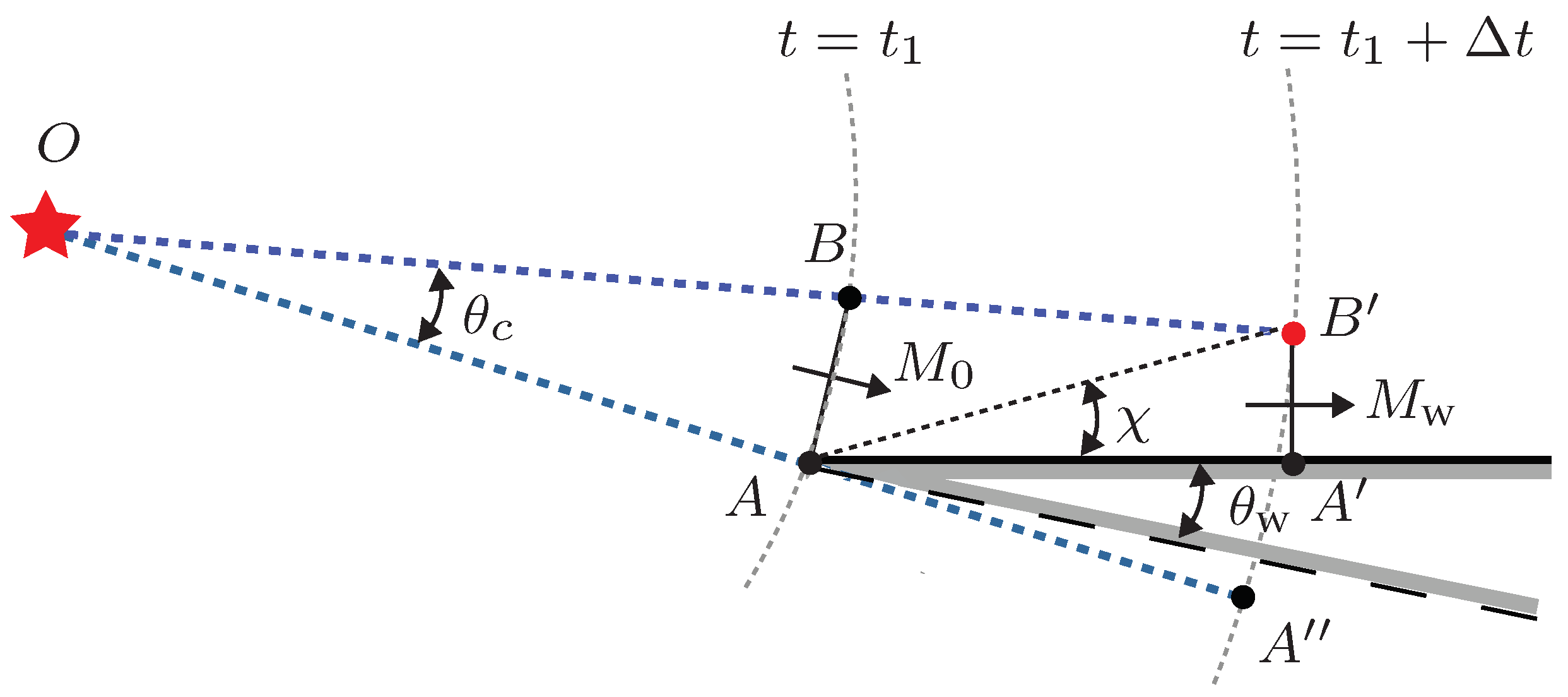
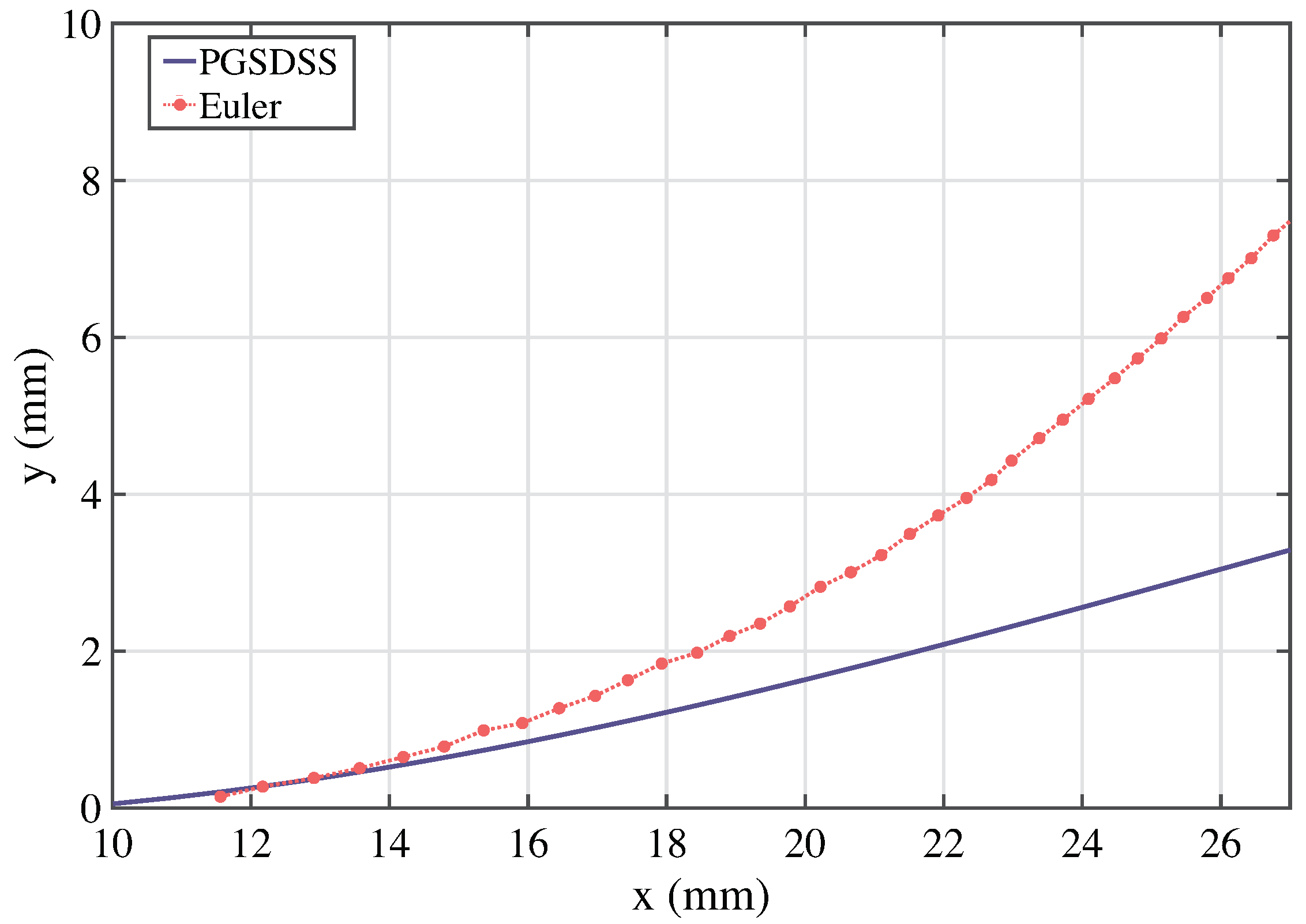
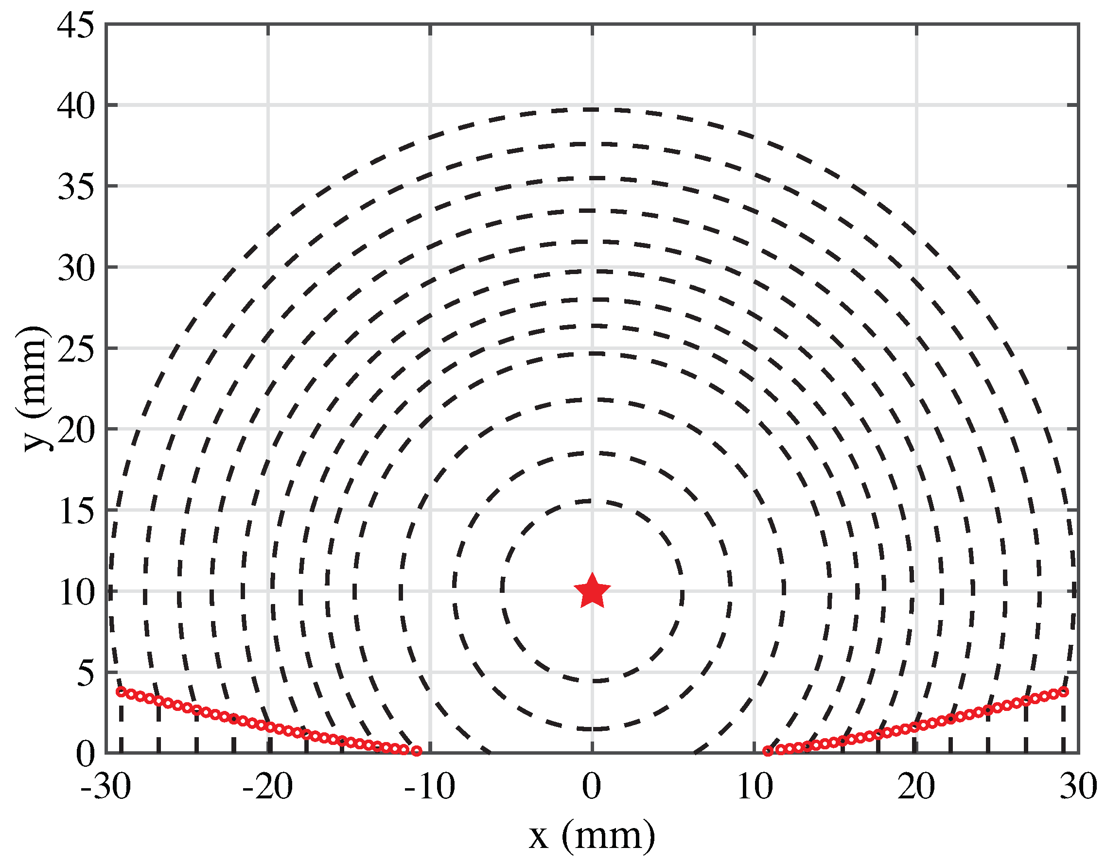
The PGSDSS model was developed aiming at overcoming the issue of GSD and PGSD overestimating the Mach stem development in the case of two cylindrical symmetrical interacting blast waves. The PGSD model treats regular and irregular reflection in different manners. In contrast, the PGSDSS model introduced in this study can be initialized with two separated blast waves represented by two closed circles in two-dimensional space. Once the shock fronts expand such that the two circular curves meet, regular reflection is realized by applying boundary conditions such that a perfect circular shape can be preserved near the intersections. Irregular reflection follows as soon as a pre-defined transition condition is reached. Mach stem growth is then governed by the shock–shock approximate theory for cylindrical shock reflection off a straight wall, while the undisturbed part of the shock front is still described by the PGSD model. The so-called PGSDSS model was evaluated by comparing the triple-point trajectory to results from simulations of the Euler equations for the interaction of two identical cylindrical blast waves. As a result, the PGSDSS model yielded almost a straight line of trajectory in the $xy$-plane that lies lower than its Euler solution counterpart at all times, which signals an underestimated Mach stem throughout its development. This observation is opposite to that from the PGSD model, which instead overestimated the Mach stem growth. One possible cause is the assumption of a straight Mach stem made in deriving the shock–shock approximate theory.

In the future, it would be beneficial to further compare the PGSD and PGSDSS models to additional experimental data obtained with high-resolution measurement equipment, such as ultra high speed cameras and pressure sensors.

References

1. Courant, R.; Friedrichs, K.; Lewy, H. On the partial difference equations of mathematical physics. IBM J. Res. Dev. 1967, 11, 215–234. [Google Scholar] [CrossRef]
2. Whitham, G.B. A new approach to problems of shock dynamics Part I Two-dimensional problems. J. Fluid Mech. 1957, 2, 145–171. [Google Scholar] [CrossRef]
3. Whitham, G.B. A new approach to problems of shock dynamics Part 2. Three-dimensional problems. J. Fluid Mech. 1959, 5, 369–386. [Google Scholar] [CrossRef]
4. Whitham, G.B. Linear and Nonlinear Waves; John Wiley & Sons: New York, NY, USA, 1974; Volume 42. [Google Scholar]
5. Cates, J.E.; Sturtevant, B. Shock wave focusing using geometrical shock dynamics. Phys. Fluids 1997, 9, 3058–3068. [Google Scholar] [CrossRef]
6. Ridoux, J.; Lardjane, N.; Monasse, L.; Coulouvrat, F. Comparison of geometrical shock dynamics and kinematic models for shock-wave propagation. Shock Waves 2018, 28, 401–416. [Google Scholar] [CrossRef]
7. Chester, W. The quasi-cylindrical shock tube. Lond. Edinb. Dublin Philos. Mag. J. Sci. 1954, 45, 1293–1301. [Google Scholar] [CrossRef]
8. Chisnell, R.F. The motion of a shock wave in a channel, with applications to cylindrical and spherical shock waves. J. Fluid Mech. 1957, 2, 286–298. [Google Scholar] [CrossRef]
9. Whitham, G.B. A note on shock dynamics relative to a moving frame. J. Fluid Mech. 1968, 31, 449–453. [Google Scholar] [CrossRef]
10. Qiu, S. Numerical Study of Focusing Effects Generated by the Coalescence of Multiple Shock Waves. Ph.D. Thesis, University of Southern California, Los Angeles, CA, USA, 2017. [Google Scholar]
11. Best, J.P. A generalisation of the theory of geometrical shock dynamics. Shock Waves 1991, 1, 251–273. [Google Scholar] [CrossRef]
12. Peace, J.T.; Lu, F.K. On the propagation of decaying planar shock and blast waves through non-uniform channels. Shock Waves 2018, 28, 1223–1237. [Google Scholar] [CrossRef]
13. Ridoux, J.; Lardjane, N.; Monasse, L.; Coulouvrat, F. Extension of geometrical shock dynamics for blast wave propagation. Shock Waves 2020, 30, 563–583. [Google Scholar] [CrossRef]
14. Bdzil, J.B.; Stewart, D.S. Modeling two-dimensional detonations with detonation shock dynamics. Phys. Fluids A Fluid Dyn. 1989, 1, 1261–1267. [Google Scholar] [CrossRef]
15. Lieberthal, B.; Stewart, D.S.; Hernández, A. Geometrical shock dynamics applied to condensed phase materials. J. Fluid Mech. 2017, 828, 104. [Google Scholar] [CrossRef]
16. Henshaw, W.D.; Smyth, N.F.; Schwendeman, D.W. Numerical shock propagation using geometrical shock dynamics. J. Fluid Mech. 1986, 171, 519–545. [Google Scholar] [CrossRef]
17. Schwendeman, D.W. A numerical scheme for shock propagation in three dimensions. Proc. R. Soc. Lond. A Math. Phys. Sci. 1988, 416, 179–198. [Google Scholar]
18. Qiu, S.; Liu, K.; Eliasson, V. Parallel implementation of geometrical shock dynamics for two dimensional converging shock waves. Comput. Phys. Commun. 2016, 207, 186–192. [Google Scholar] [CrossRef]
19. Schwendeman, D.W. Numerical shock propagation in non-uniform media. J. Fluid Mech. 1988, 188, 383–410. [Google Scholar] [CrossRef]
20. Ridoux, J.; Lardjane, N.; Monasse, L.; Coulouvrat, F. Beyond the limitation of Geometrical Shock Dynamics for diffraction over wedges. Shock Waves 2019, 29, 833–855. [Google Scholar] [CrossRef]
21. Schwendeman, D.W. A higher-order Godunov method for the hyperbolic equations modelling shock dynamics. Proc. R. Soc. Lond. Ser. A Math. Phys. Eng. Sci. 1999, 455, 1215–1233. [Google Scholar] [CrossRef]
22. Schwendeman, D.W. On converging shock waves of spherical and polyhedral form. J. Fluid Mech. 2002, 454, 365. [Google Scholar] [CrossRef]
23. Noumir, Y.; Le Guilcher, A.; Lardjane, N.; Monneau, R.; Sarrazin, A. A fast-marching like algorithm for geometrical shock dynamics. J. Comput. Phys. 2015, 284, 206–229. [Google Scholar] [CrossRef]
24. Gottlieb, S.; Shu, C.W. Total variation diminishing Runge-Kutta schemes. Math. Comput. 1998, 67, 73–85. [Google Scholar] [CrossRef]
25. Bach, G.G.; Lee, J.H.S. An analytical solution for blast waves. AIAA J. 1970, 8, 271–275. [Google Scholar] [CrossRef]
26. Henshaw, W.D. Overture: An Object-Oriented Toolkit for Solving Partial Differential Equations in Complex Geometry. Available online: https://www.overtureframework.org/ (accessed on 21 September 2023).
27. Brown, D.; Henshaw, W.; Quinlan, D. Overture: An object-oriented framework for solving partial differential equations on overlapping grids. In Object Oriented Methods for Interoperable Scientific and Engineering Computing, Proceedings of the 1998 SIAM Workshop; SIAM: Philadelphia, PA, USA, 1999; pp. 245–255. [Google Scholar]
28. Chesshire, G.; Henshaw, W. omposite overlapping meshes for the solution of partial differential equations. J. Comput. Phys. 1990, 90, 1–64. [Google Scholar] [CrossRef]
29. Henshaw, W.; Schwendeman, D. Parallel computation of three-dimensional flows using overlapping grids with adaptive mesh refinement. J. Comput. Phys. 2008, 227, 7469–7502. [Google Scholar] [CrossRef]
30. Godunov, S.K. A difference scheme for numerical solution of discontinuous solution of hydrodynamic equations. Math. Sb. 1959, 47, 271–306. [Google Scholar]
31. Taylor, G.I. The formation of a blast wave by a very intense explosion I. Theoretical discussion. Proc. R. Soc. Lond. Ser. A Math. Phys. Sci. 1950, 201, 159–174. [Google Scholar]
32. Lin, S.C. Cylindrical shock waves produced by instantaneous energy release. J. Appl. Phys. 1954, 25, 54–57. [Google Scholar] [CrossRef]
33. Yoo, S.; Butler, G.C. New GSD Modeling for Air Blast Wave Supported by Non-Uniform Flow: I. Modeling; Technical Report; Air Force Research Lab, Munitions Directorate, Eglin AFB: Valparaiso, FL, USA, 2019. [Google Scholar]
34. Higashino, F.; Henderson, L.F.; Shimizu, F. Experiments on the interaction of a pair of cylindrical weak blast waves in air. Shock Waves 1991, 1, 275–284. [Google Scholar] [CrossRef]
35. Hornung, H.G.; Oertel, H.; Sandeman, R.J. Transition to Mach reflection of shock waves in steady and pseudo steady flow with and without relaxation. J. Fluid Mech. 1979, 90, 541–560. [Google Scholar] [CrossRef]
36. von Neumann, J. Collected Works; Pergamon Press: Oxford, UK, 1963; Volume 6. [Google Scholar]
37. Schwendeman, D.W.; Whitham, G.B. On converging shock waves. Proc. R. Soc. Lond. Ser. A Math. Phys. Sci. 1987, 413, 297–311. [Google Scholar]
Figure 1. M-R plots of the propagation of a single cylindrical blast in air. Initial conditions: E 0 = 8000 J/m for the Euler and analytical solutions, and initial conditions R 0 = 10 mm with either M 01 = 11.81 or M 02 = 9.76 for GSD solutions.
Aerospace 10 00838 g001
Figure 2. Geometrical terms and post-shock flow terms are plotted as functions of the blast radius. Initial conditions: R 0 = 10 mm and M 0 = 9.76 for the first-order complete GSD and modified GSD solutions.
Aerospace 10 00838 g002
Figure 3. M-R plots of the propagation of a single cylindrical blast in air for different GSD models. Initial conditions: E 0 = 8000 J/m for the analytical solution; R 0 = 10 mm and M 0 = 9.76 for the GSD, 1 st -order complete GSD, modified GSD, and PGSD solutions.
Aerospace 10 00838 g003
Figure 4. Schematic illustration of the experiments of [34], in which the exploding wire centers (represented by red stars) are located 60 mm apart from each other. The wedge angle is represented by θ w .
Aerospace 10 00838 g004
Figure 5. Ratio of maximum pressure at the Mach stem, P m , to ambient pressure, P a , as a function of time. Modified GSD data are reproduced from [10], which also provided the initial conditions to the current PGSD simulations referred to as I.C.1.
Aerospace 10 00838 g005
Figure 6. Time history of the shock front as a function of the radius using initial conditions I.C.2.
Aerospace 10 00838 g006
Figure 7. Ratio of maximum pressure at the Mach stem, P m , to ambient pressure, P a , as a function of time. Experimental data reproduced from [34] with permission from Springer.
Aerospace 10 00838 g007
Figure 8. Schematic illustration of Whitham’s application of GSD to diffraction of a planar shock by a straight wedge. Triple points are represented by red dots.
Aerospace 10 00838 g008
Figure 9. Schematic illustration of the diffraction of a planar shock interaction with a straight surface. Triple points are represented by red dots.
Aerospace 10 00838 g009
Figure 10. Schematic illustration of the diffraction of a cylindrical shock interaction with a straight surface. Triple points are represented by red dots.
Aerospace 10 00838 g010
Figure 11. Comparison of the trajectory of the triple point for the interaction between two identical cylindrical blasts from the Euler (solid line) and PGSDSS (dashed line with circles) solutions. Initial conditions: E 0 = 10 , 000 J/m for the Euler solution; R 0 = 5 mm and M 0 = 26.7 for the PGSDSS solution.
Aerospace 10 00838 g011
Figure 12. PGSDSS results showing the evolution of the shock front formed by the interaction between two identical cylindrical blast waves. Only half of the shock fronts shown with triple points represented by red circles, and the explosion center indicated by a red star. Initial conditions: R 0 = 5 mm and M 0 = 26.7 .
Aerospace 10 00838 g012
Disclaimer/Publisher’s Note: The statements, opinions and data contained in all publications are solely those of the individual author(s) and contributor(s) and not of MDPI and/or the editor(s). MDPI and/or the editor(s) disclaim responsibility for any injury to people or property resulting from any ideas, methods, instructions or products referred to in the content.