A Pattern Search Method to Optimize Mars Exploration Trajectories

Abstract

The Korean National Space Council recently released “Mars Exploration 2045” as part of its future strategic plan. The operations for a Mars explorer can be defined based on domestically available capabilities, such as ground operations, launch, in-space transport and deep space link. Accordingly, all of our exploration scenarios start from the Naro space center, and the pathway to Mars is optimized using an objective function that minimizes the required ∆V. In addition, the entire phase of Mars orbit insertion should remain in contact with our deep space antennas, a measure that is imposed as an operational constraint. In this study, a pattern search method is adopted, as it can handle a nonlinear problem without relying on the derivatives of the objective function, and optimal trajectories are generated on a daily basis for a 15-day launch period. The robustness of this direct search method is confirmed by consistently converged solutions showing, in particular, that the ascending departure requires slightly less ∆V than the descending departure on the order of 10 m/s. Subsequently, mass estimates are made for a Mars orbiter and a kick stage to determine if the desired ∆V is achievable with our eco-friendly in-space propulsion system when launched from our indigenous launch vehicle, KSLV-II.

1. Introduction

In 2023, Korea space launch vehicle II (KSLV-II) successfully transported multiple satellites into orbit after two test flights, and the Korean pathfinder lunar orbiter (KPLO) made a lunar orbit insertion with no glitches. These two events symbolize that a new era of independent access to space and space exploration has opened up in Korea. Indeed, the national space council released a brand-new version of the basic plan for space development and promotion, which contains a strategic plan for independently sending a lander to Mars by 2045 [1].

Around the world, Mars exploration is being pursued to investigate the presence of water on Mars and to gather clues about the origin and formation processes of the solar system. Since NASA’s Mariner 4 first reached Mars in 1964, global efforts have been made to explore Mars, including the Mars reconnaissance orbiter (MRO) in 2005 and the Mars atmosphere and volatile evolution (MAVEN) in 2013 [2,3]. Europe has sent missions such as Mars Express in 2003 and ExoMars in 2016; India launched Mangalyaan in 2013; the UAE conducted the Emirates Mars Mission (EMM) in 2020; and China sent Tianwen-1 to Mars in 2020 [4,5,6,7,8]. In this situation, South Korea needs to determine what kind of Mars exploration is possible based on our infrastructure, such as the launch site and deep space link in our country, as well as the recently developed KSLV-II and eco-friendly in-space propulsion system for exploration.

When examining the porkchop plot by solving Lambert’s problem for Mars exploration, it shows that the opportunities to travel from Earth to Mars occur approximately every two years, and the time of flight (TOF) typically requires 6 to 10 months [9]. Despite the periodic nature of launch opportunities, the Earth departure energy (${\mathrm{C}}_3$) and Mars arrival excessive velocity (${\mathrm{V}}_{\mathrm{\infty }}$), which directly affect the velocity increment (∆V), exhibit different distributions each time. This is because Earth and Mars do not have circular orbits centered around the Sun and they are not in the same orbital plane [10]. In this study, we aimed to set a specific launch period under these circumstances and determine daily trajectories that allow fuel minimization and meet the operational constraints.

The research on trajectory optimization mainly focuses on minimizing fuel consumption or the TOF. Abdelkhaik developed a non-coplanar trajectory design using impulsive burn and the genetic algorithm; Vasile optimized Earth–Mars trajectories using the evolutionary-branching technique; and Ellipson applied an analytical method to calculate the derivatives of the dynamic model for optimizing a comet sample return mission [11,12,13]. Miele and Filho optimized Earth–Mars trajectories using the sequential gradient-restoration algorithm [14,15]; however, these methods mainly involved complex computations and were challenging to use to model nonlinear constraints like operational constraints since they relied on techniques such as impulsive burn and partial derivatives of the dynamic model. Recently, as artificial intelligence has been actively researched, Izzo applied artificial intelligence techniques to interplanetary trajectories, but it had limitations in that the specific applicability was unclear and the data set for learning was insufficient [16].

The mentioned research cases mostly assume multiple impulsive burns for Mars trajectory optimization; however, in reality, when performing Mars orbit insertion (MOI) using the in-space onboard propulsion system, it is necessary to model it as a finite burn since the propulsion system cannot produce a momentary high thrust. Furthermore, there exists a strong operational constraint that Earth’s deep space antennas should remain in contact with the propulsion system for entire burn duration of the MOI to perform the orbit determination and to estimate the propulsion system’s performance. In order to address the high cost and long-term environmental concerns associated with toxic propellants, a propulsion system utilizing hydrogen peroxide–kerosene as a propellant was developed. The eco-friendly propulsion system provides a thrust of 500 N and a specific impulse of 306.5 s. When this propulsion system was applied to the Mars explorer, it was confirmed that the explorer could enter Mars orbit within a period of 35 h in a single finite burn. This highlights the importance of developing eco-friendly propulsion systems, as they offer a viable alternative for space missions while minimizing the environmental impacts and cost concerns associated with toxic propellants.

For Mars exploration trajectory, we applied the pattern search method, which is one of the direct search techniques, to find the global optimum of the objective function without computing the derivatives [17,18]. Additionally, we formulated the problem by imposing excessive penalties when an operational constraint is not satisfied during the iterative computation process, ensuring that such nonlinear constraints are satisfied. Based on the scenario of departing to Mars in December 2030, we generated daily optimal trajectories within a 15-day launch period using the pattern search method. We confirmed that the pattern search method showed relatively robust convergence while not requiring many sub-function calls. Above all, we calculated different types of Mars transfer trajectories: one that passes over the Earth’s North Pole (ascending departure) and another one that passes over the South Pole (descending departure) after trans-mars injection (TMI) by selecting launch times that are 12 h apart and have different coasting durations in Earth’s parking orbit. As a result, we determined that the ascending departure provides less ∆V than the descending departure on the order of 10 m/s.

Furthermore, we derived the required ∆V for the kick stage and the new Mars explorer and established a ∆V budget by considering trajectory correction maneuvers, aerobraking maneuvers and other margins. Subsequently, we found that the minimum mass of the Mars explorer that can be loaded onto KSLV-II is approximately 348.9 kg, and the dry mass of the explorer is around 203.8 kg. As this study has demonstrated that by employing the optimal trajectory design for not only the ground operations and in-space transport, but also the non-toxic propulsion system and deep space antenna for monitoring the MOI burn, South Korea can realistically carry out Mars exploration.

Section 2 describes the key infrastructure for Mars exploration, including the Naro Space Center, KSLV-II, an eco-friendly propulsion system and deep space link. In Section 3, the results of the Lambert problem are provided, which are necessary to obtain the distribution of Earth departure energy, Mars arrival velocity and the right ascension and declination of the launch asymptote for the Mars exploration in December 2030. Furthermore, specific phases for the exploration are described. This section also elaborates on the dynamics model and orbital propagation model, and it explains the differential corrections process and pattern search method to solve optimization problems. Section 4 describes the convergence process of the direct search method and detailed simulation results relative to the converged TOF, TMI ∆V, MOI ∆V and coverage status during MOI. In addition, the specific mass of the upper stage of the launch vehicle and the mass of the Mars explorer are estimated considering realistic situations. Finally, Section 5 summarizes the overall conclusions.

2. Infrastructure for Mars Exploration

South Korea has been carrying out systematic projects for space exploration, starting with the construction of a launch facility and the simultaneous development of launch vehicles. With the successful second launch of KSLV-II on 21 June 2022, designed to transport medium-sized satellites into low Earth orbit, and the successful third launch on 25 May 2023, South Korea has achieved the capability for substantial space transportation. Additionally, KPLO, launched on 5 August 2022, is currently operating in lunar orbit, and the Korea deep space antenna (KDSA) was established to track and facilitate two-way communication with KPLO. At universities, the development of eco-friendly propulsion systems is causing a new shift in the space exploration paradigm, which has traditionally relied on toxic propellants.

2.1. Naro Space Center and KSLV-II

The Naro Space Center (34.43° N, 127.53° E) was established in 2009 in Goheung, South Jeolla province, in the southern part of South Korea, with the purpose of launching domestically developed launch vehicles. Until 2013, KSLV-I was mainly launched from this center, and recently, the third launch of KSLV-II was carried out. There are plans to launch a lunar lander in 2032 using KSLV-III. To support these missions, the Naro Space Center is equipped with a launch complex, propulsion test facilities, mission control and administration center and tracking radar, as well as assembly and test facilities, as shown in Figure 1. Although the Naro Space Center is located at mid-latitudes in the northern hemisphere, the available launch azimuth is approximately 172° due to range safety requirements and non-yaw maneuvers during the ascent of the launch vehicle, which would ensure that the parking orbit inclination after separation would be approximately 80° [19].

KSLV-II is three-staged with turbo-pump types and is based on the 75-tonf class and 7-tonf class. Its length and diameter are 47.5 m and 3.5 m, respectively. The design parameters of KSLV-II are described in

Table 1. Design parameters of KSLV-II.

Parameter	1st Stage	2nd Stage	3rd Stage
Length	21.6 m	13.6 m	3.5 m
Mass	143 ton	42.3 ton	12.6 ton
Vacuum thrust	300-tonf (75-tonf × 4)	75-tonf	7-tonf
Vacuum specific impulse	298.5 s	315.9 s	326.6 s
Operating time	126 s	144 s	500 s

. The payload mass in the parking orbit launched by KSLV-II is 2600 kg, while the payload consists of the upper stage (4th stage) and spacecraft. The upper stage is a spin-stabilized solid rocket, and the thruster force and the specific impulse are 7-tonf and 287.5 s, respectively [20,21]. This information is used to estimate the mass of the upper stage in Section 4.2.

2.2. Eco-Friendly Hypergolic Propulsion System

Since 2010 in South Korea, green (or nontoxic) hypergolic propellants have been researched as one of the options for future space propulsion. The motivation for green hypergolic propulsion is not only to reduce the costs of the technical development procedure but also to ensure the safety of personnel and equipment. Hydrogen peroxide (H₂O₂) is considered a green oxidizer owing to its environmentally friendly nature [22]. Various types of reactive fuels have been developed. Among the candidates, few combinations have been tested for applicability to a pressure-fed system of small-scale liquid thrusters [23]. The whole system schematic diagram is shown in Figure 2, and the successful demonstration through ground hot-firing tests using a 500 N-scale engineering model thruster (stock 2 fuel and 90 wt.% H₂O₂ oxidizer) is shown in Figure 3.

Stock 2 fuel is a mixture of energetic hydrocarbon chemicals: tetraglyme, tetrahydrofuran and toluene. All the chemicals are readily available in the commercial market. A small amount of sodium borohydride is added to the fuel as an ignition source. The significantly meaningful feasibility of the concept of green hypergolic propellants was first proven in South Korea. When the concentration of H₂O₂ is 98 wt.%, the ignition delay of the hypergolic combination is comparable to that of the conventional toxic combination (monomethylhydrazine/nitrogen tetroxide). As shown in

Table 2. Design parameters of a 500 N-scale green hypergolic bipropellant thruster.

Parameter	Value
Oxidizer	90 wt.% H2O2
Reactive fuel	Stock 2
Design thrust	500 N
Design chamber pressure	30 bar
Ideal vacuum specific impulse ($I_{sp}$)	306.5 s
Ideal characteristic velocity (C*)	1579.2 m/s
Theoretical oxidizer to fuel ratio	5.48
Design mass flow rate	Oxidizer: 131.4 g/s, fuel: 24.0 g/s

, the equilibrium specific impulse of the green hypergolic combination, stock 2 and 90 wt.% H₂O₂, theoretically approaches 306.5 s in a vacuum if the chamber pressure of the thruster is set to 30 bar.

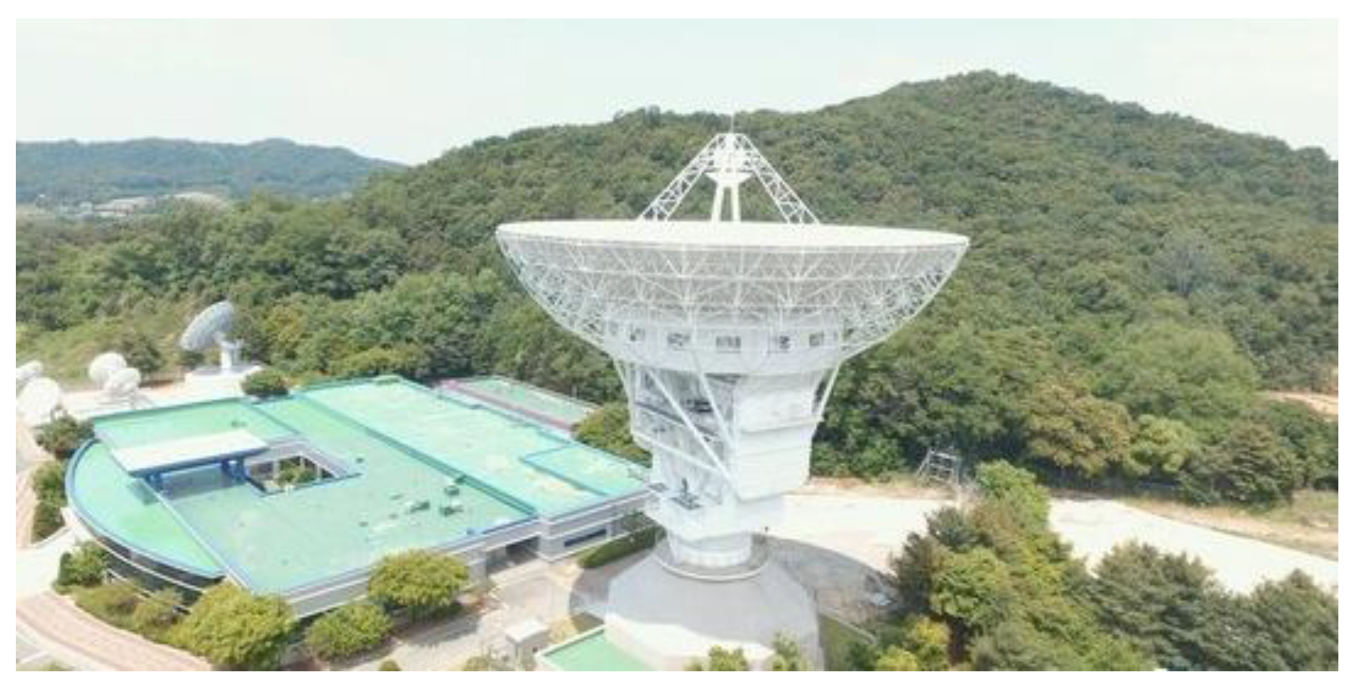
2.3. Korea Deep Space Antenna

For communication with the Mars explorer, the KDSA is located in the satellite center in Yeoju (37.21° N, 127.62° E) and is currently operating to track and communicate with the deep space mission. As shown in Figure 4, the size of this antenna is approximately 35 m, and it has the ability to send telecommands and receive telemetry signals using the S/X-band [24]. A full coverage constraint during the MOI is imposed in the mission design and a 5° elevation constraint is also applied to the pass plan between them.

3. Problem Description

There is a plan to send a Mars lander in 2045, but realistically, it is necessary to first send an orbiter to Mars for technical validation. In this study, among the five regular opportunities to travel to Mars between 2028 and 2035, we assume that the orbiter will be sent to Mars in December 2030, which requires the second highest ∆V [25]. The reason is that if we choose an opportunity with a lower ∆V required initially, but then miss that opportunity and move on to the next one, it may result in higher ∆V demands, requiring us to reduce the mass of the spacecraft.

To design the Mars mission trajectory, a patched-conic approximation based on Lambert’s problem was utilized. The mission scenario is divided into three stages: Earth departure phase, Mars transfer phase and MOI phase. The problem was formulated using several differential corrections problems to ensure that the explorer arrives at the mission orbit of Mars from the Naro Space Center. The pattern search method was applied to complete coverage for the MOI burn, as well as to minimize the required ∆V simultaneously.

3.1. Solution of Lambert’s Problem

There are four opportunities (two Type I and two Type II) to go to Mars between late 2030 and early 2031 [25]. Among the opportunities, a departure date in late 2030 (Type II) was selected because this case requires the minimum arrival excessive velocity (${\mathrm{V}}_{\mathrm{\infty }}$) compared to the other cases, which directly affects the MOI ∆V. Figure 5 shows the departure energy (${\mathrm{C}}_3$) and arrival excessive velocity during Earth–Mars ballistic transfer trajectories departing in late 2030 and arriving in late 2031 solved by Lambert’s problem [9]. It also shows the declination (DLA, ${\delta }_{Dep}$) and right ascension (RLA, ${\alpha }_{Dep}$) of the launch asymptote, which provide the flight direction of the explorer to reach Mars after separation according to given departure and arrival dates.

3.2. Mars Exploration Scenario

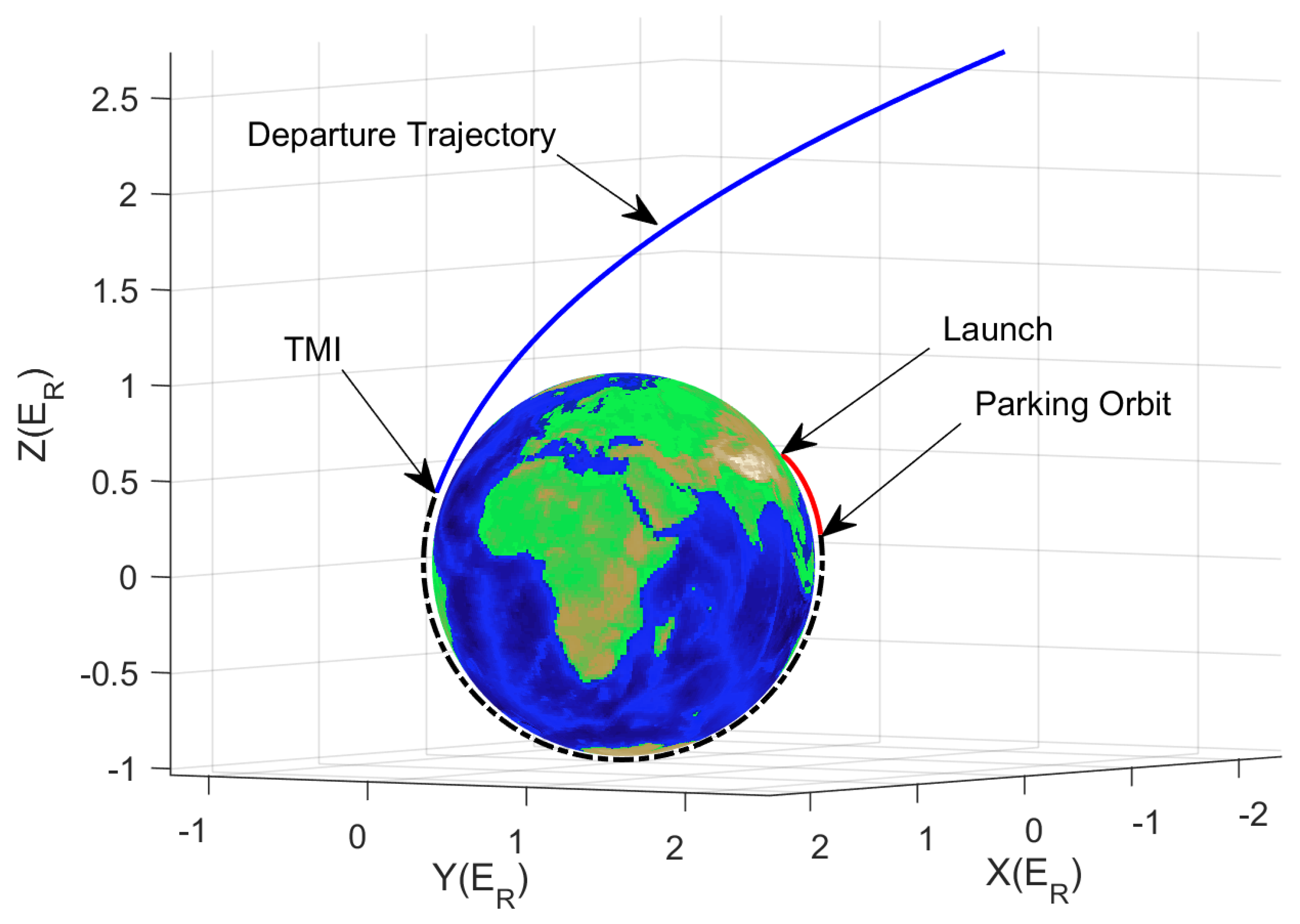
3.2.1. Earth Departure Phase

The launch to TMI occurs at the Naro Space Center, and the KSLV-II puts the payload into the parking orbit with an altitude of 300 km and an inclination of 80° for an ascent duration of 870 s. The launch trajectory is generated by using the boundary value problem of the KSLV-II data for the initial states (−3208.567 km, 4176.19 km, 3586 km, 0.0 km/s, 0.0 km/s, 0.0 km/s) and final states (−4341.062 km, 4985.920 km, 942.112 km, −1.3632 km/s, 0.2360 km/s −7.5307 km/s) with respect to Earth-centered fixed coordinates [26]. Once the payload is put into parking orbit, it has a coast duration ($∆{\mathrm{t}}_{\mathrm{C}\mathrm{o}\mathrm{a}\mathrm{s}\mathrm{t}}$), and then it executes the TMI burn ($∆{\mathrm{V}}_{\mathrm{T}\mathrm{M}\mathrm{I}}$) using the upper stage; however, by adjusting the launch epoch and the coast duration in the parking orbit, it is possible to distinguish a Mars transfer trajectory where the spacecraft passes over the Earth’s North Pole (ascending departure) or South Pole (descending departure) after TMI. This phenomenon is a result of the Earth’s rotation. To satisfy these conditions, the time difference between the launch epochs for these two cases is approximately 12 h. Figure 6 shows the ascending departure that consists of a launch trajectory from Naro Space Center (red solid line), coast duration trajectory (around 50 min) in parking orbit (black dot line) and trans-Mars trajectory after TMI (blue solid line).

3.2.2. Mars Transfer Phase

This phase is from after TMI to the approach to Mars, as shown in Figure 7. A Mars explorer needs to deploy solar panels and a high-gain antenna after separation. Based on priority, the attitude will be controlled, the orbit determination will be performed, the state of health will be checked, the onboard computer will be configured, the onboard propulsion system will be calibrated and the instrument will be baked out. Several trajectory correction maneuvers (TCMs) will be performed, and the MOI will be prepared in this phase. There are two approaches to Mars: the south pole approach and the north pole approach. Since the condition of the Mars approach does not have a meaningful impact on the required ∆V [15], the Mars’ south pole approach was selected due to the better coverage geometry between the ground antenna and explorer during MOI than the north pole approach.

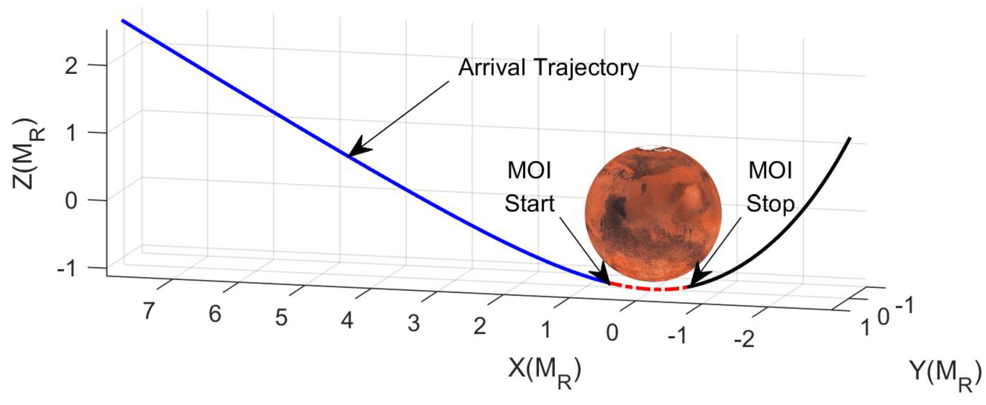
3.2.3. Mars Orbit Insertion Phase

In this phase, the Mars explorer should be captured by the predefined orbital period using the eco-friendly propulsion system. For this maneuver, a finite burn with attitude hold is modeled and the KDSA should monitor all the MOI burn durations. Therefore, the Mars arrival time should be carefully selected to not only cover the entire MOI duration but minimize the required ∆V. Figure 8 shows the hyperbolic arrival trajectory (blue solid line), MOI burn duration (red dot line) and captured orbit after MOI (black solid line). Targeting Mars orbital elements after MOI are a periapsis altitude ($h_M$) of 425 km, inclination ($i_M$) of 90° and orbital period ($T_M$) of 35 h, which are same values as those used for MRO [2]. In order to perform meaningful scientific missions, it is necessary to reach an orbit with an approximately 2 h period. To achieve this, the aerobraking method similar to MRO, which takes around 6 months but allows for fuel-saving, is assumed [27].

3.3. Dynamic and Propagation Models

The equations of motion in this problem can be written as follows [28]: the first term of Equation (1) describes Newton’s formulation of gravitation of two orbiting bodies, the second term describes the third-body gravitational perturbation, and the third term represents other forces affecting the Mars explorer.

$$\ddot{\mathbf{r}}=-\mu \frac{\mathbf{r}}{{‖\mathbf{r}‖}^3}+\sum _{i>0}{\mu }_i\left(\frac{{\mathbf{r}}_{Bi}-\mathbf{r}}{{‖{\mathbf{r}}_{Bi}-\mathbf{r}‖}^3}-\frac{{\mathbf{r}}_{Bi}}{{‖{\mathbf{r}}_{Bi}‖}^3}\right)+\frac{1}{m}{\mathbf{F}}_s$$

(1)

where $\ddot{\mathbf{r}}$ and $\mathbf{r}$ are the acceleration and position of the spacecraft relative to a coordinate system with origin $B_0$. $\mu$ and ${\mu }_i$ are the gravitational parameters for $B_0$ (reference gravitational body) and $B_i$ (i^th gravitational body). ${\mathbf{r}}_{Bi}$ is the position of $B_i$ relative to $B_0$. This problem deals with multiple bodies; for example, if the explorer is within the sphere of influence (SOI) of the Earth, $\mu$ should use Earth’s gravitational parameters and ${\mu }_i$ should be other bodies, such as the Sun, Moon, Mars and Jupiter, as described in

Table 3. Propagation models for three phases.

Model	Earth Departure Phase	Mars Transfer Phase	MOI Phase
Gravitational field ($\mu$)	WGS84-EGM96 21 × 21	Sun point mass	MRO110C 8 × 8
Atmospheric drag	Jacchia–Roberts	-	Mars Gram 2010
Solar radiation pressure	Dual cone	Dual cone	Dual cone
Third bodies (${\mu }_i$)	Sun, Moon, Mars	Earth, Mars, Jupiter	Earth, Sun, Jupiter
SOI distance	925,000 km	-	577,000 km

. $m$ is the mass of the spacecraft, and ${\mathbf{F}}_s$ consists of atmospheric drag and the solar radiation pressure force. Atmospheric drag is modeled if the explorer is within the SOI of Earth and Mars. The drag coefficient in Earth orbit is assumed to be 2.2 [29] and the drag coefficient in Mars orbit is assumed to be 2.2 based on the accelerometer data of MAVEN and Mars Odyssey when the atmosphere density was lower than 1 × 10⁻³ [30]. The SRP coefficient is assumed to be 1.0. The cross-sectional area is assumed to be 4 m², and the mass of the Mars explorer ($m$) after TMI is 348.9 kg, which will be described in Section 4.2. For propagation, a 7th order Runge–Kutta–Fehlberg integrator with an 8th order error control and variable step size control was used. The integrator uses an absolute error tolerance of 1 × 10⁻¹⁰ and a relative error tolerance of 1× 10⁻¹³.

3.4. Differential Corrections Process

A differential corrections process using the Newton–Raphson method, which is a root-finding algorithm to design the trajectory of the Mars mission, is used [31]. The mathematical representation of this problem is described in Equation (2). $\mathbf{x}$ represents the independent variables, ${\mathbf{y}}_{\mathrm{d}}$ represents the equality constraints and $\mathbf{f}\left(\mathbf{x}\right)$ involves propagation using Equation (1).

$$\tilde{\mathbf{y}}=\mathbf{f}\left(\mathbf{x}\right)-{\mathbf{y}}_{\mathrm{d}}=0$$

(2)

The initial conditions (${\mathbf{x}}_0$) are applied to integrate $\mathbf{f}\left(\mathbf{x}\right)$ and then compare with ${\mathbf{y}}_{\mathrm{d}}$ to find the independent variables ($\mathbf{x}$). If the difference ($\tilde{\mathbf{y}}$) is not zero, the iteration process is performed until it meets the predefined tolerance. For evaluation of the next step, as shown in Equation (3), the first derivative of $\mathbf{f}\left(\mathbf{x}\right)$ is calculated and a numerical approach should be applied using small perturbation ($\mathsf{\delta }\mathbf{x}$) to calculate the first derivative of $\mathbf{f}\left(\mathbf{x}\right)$ analytically.

$${\mathbf{x}}_{\mathrm{k}+1}={\mathbf{x}}_{\mathrm{k}}-{\mathbf{J}}_{\mathbf{n}}^{-1}\left(\mathbf{f}\left({\mathbf{x}}_{\mathrm{k}}\right)-{\mathbf{y}}_{\mathrm{d}}\right)$$

(3)

The first derivative of $\mathbf{f}\left(\mathbf{x}\right)$ is called the Jacobian matrix, which consists of the partial derivatives, as shown Equation (4), and the i^th component is ${\mathbf{J}}_{\mathrm{i}}=(\mathbf{f}\left(\mathbf{x}+\mathsf{\delta }{\mathbf{x}}_{\mathrm{i}}\right)-\mathbf{f}\left(\mathbf{x}\right))/\mathsf{\delta }{x}_i.$

$$\mathbf{J}=\left[\begin{array}{ccc}\frac{{\partial \mathrm{y}}_1}{{\partial \mathrm{x}}_1}& \cdots & \frac{{\partial \mathrm{y}}_1}{{\partial \mathrm{x}}_{\mathrm{n}}}\\ ⋮& \ddots & ⋮\\ \frac{{\partial \mathrm{y}}_{\mathrm{m}}}{{\partial \mathrm{x}}_1}& \dots & \frac{{\partial \mathrm{y}}_{\mathrm{m}}}{{\partial \mathrm{x}}_{\mathrm{n}}}\end{array}\right]$$

(4)

Table 4. Definition of the targeting problems using differential corrections process.

Targeting Name	$\mathbf{Variable}(\mathbf{x})$	$\mathbf{Initial}\mathbf{Value}\left({\mathbf{x}}_0\right)$	$\mathbf{Constraint}\left({\mathbf{y}}_{\mathbf{d}}\right)$	Constraint Value
Departure	${\mathrm{t}}_{\mathrm{L}\mathrm{a}\mathrm{u}\mathrm{n}\mathrm{c}\mathrm{h}}$	19 December 2030~2 January 2031	${\mathrm{C}}_3$	10.0~12.4 km2/s2
	$∆{\mathrm{t}}_{\mathrm{C}\mathrm{o}\mathrm{a}\mathrm{s}\mathrm{t}}$	50 or 100 min	${\mathsf{\delta }}_{\mathrm{D}\mathrm{e}\mathrm{p}}$	12.1°~19.8°
	$∆{\mathrm{V}}_{\mathrm{T}\mathrm{M}\mathrm{I}}$	3.7 km/s	${\mathsf{\alpha }}_{\mathrm{D}\mathrm{e}\mathrm{p}}$	228.1°~231.2°
B-plane	${\mathrm{t}}_{\mathrm{L}\mathrm{a}\mathrm{u}\mathrm{n}\mathrm{c}\mathrm{h}}$	Converging values of “Departure” problem	${\mathrm{t}}_{\mathrm{A}\mathrm{r}\mathrm{r}\mathrm{i}\mathrm{v}\mathrm{a}\mathrm{l}}$	27 September 2031~1 November 2031
	$∆{\mathrm{t}}_{\mathrm{C}\mathrm{o}\mathrm{a}\mathrm{s}\mathrm{t}}$		${\mathrm{B}}_{\mathrm{t}}$	0.0 km
	$∆{\mathrm{V}}_{\mathrm{T}\mathrm{M}\mathrm{I}}$		${\mathrm{B}}_{\mathrm{r}}$	15,000.0 km
Mars approach	${\mathrm{t}}_{\mathrm{L}\mathrm{a}\mathrm{u}\mathrm{n}\mathrm{c}\mathrm{h}}$	Converging values of “B-plane” problem	${\mathrm{t}}_{\mathrm{A}\mathrm{r}\mathrm{r}\mathrm{i}\mathrm{v}\mathrm{a}\mathrm{l}}$	27 September 2031~1 November 2031
	$∆{\mathrm{t}}_{\mathrm{C}\mathrm{o}\mathrm{a}\mathrm{s}\mathrm{t}}$		${\mathrm{i}}_{\mathrm{M}}$	90.0°
	$∆{\mathrm{V}}_{\mathrm{T}\mathrm{M}\mathrm{I}}$		${\mathrm{h}}_{\mathrm{M}}$	425 km
MOI	$∆{\mathrm{t}}_{\mathrm{M}\mathrm{O}\mathrm{I}}$	800 s	${\mathrm{T}}_{\mathrm{M}}$	35 h

describes four targeting problems to arrive at the Mars orbit in detail. The “Departure” problem is set from launch to TMI to find three independent variables, such as the launch epoch (${\mathrm{t}}_{\mathrm{L}\mathrm{a}\mathrm{u}\mathrm{n}\mathrm{c}\mathrm{h}}$) from the Naro Space Center, coast duration ($∆{\mathrm{t}}_{\mathrm{C}\mathrm{o}\mathrm{a}\mathrm{s}\mathrm{t}}$) in the parking orbit and TMI ∆V ($∆{\mathrm{V}}_{\mathrm{T}\mathrm{M}\mathrm{I}}$) to go to Mars. If the ascending (descending) departure is determined, the initial condition for the $∆t_{\mathrm{C}\mathrm{o}\mathrm{a}\mathrm{s}\mathrm{t}}$ should be set to 50 min (100 min), as shown in Figure 6, when we launch the explorer from the Naro Space Center using KSLVL-II. Regardless of the departure selection, the equality constraints that are solutions of Lambert’s problem, such as the departure energy (${\mathrm{C}}_3$), declination (${\mathsf{\delta }}_{\mathrm{D}\mathrm{e}\mathrm{p}}$) and right ascension (${\mathsf{\alpha }}_{\mathrm{D}\mathrm{e}\mathrm{p}}$) of the launch asymptote, should be the same.

Once the “Departure” problem is solved, the next step is to solve the “B-plane” problem, which involves reaching the B-plane of Mars. Since the control variables of “B-plane” remain the same as those in the “Departure” problem, the converged control variables of the “Departure” problem are used as initial values for the “B-plane”. In this study, the coordinate system used for the B-plane is based on the Mars mean equator and International Astronomical Union vector of J2000, with the k-vector pointing towards the north pole of Mars. ${\mathrm{B}}_{\mathrm{t}}$ and ${\mathrm{B}}_{\mathrm{r}}$, along with the arrival time at Mars (${\mathrm{t}}_{\mathrm{A}\mathrm{r}\mathrm{r}\mathrm{i}\mathrm{v}\mathrm{a}\mathrm{l}}$), are set as equality constraints. According to the definition of the B-plane, the positive direction of ${\mathrm{B}}_{\mathrm{t}}$ is “rightward” and the positive direction of ${\mathrm{B}}_{\mathrm{r}}$ is “downward”.

As detailed in Table 4, we can see that the initial condition of the launch epoch (${\mathrm{t}}_{\mathrm{L}\mathrm{a}\mathrm{u}\mathrm{n}\mathrm{c}\mathrm{h}}$) has a range from 19 December 2030 to 2 January 2031, and the constraint values of ${\mathrm{C}}_3$, ${\mathsf{\delta }}_{\mathrm{D}\mathrm{e}\mathrm{p}}$ and ${\mathsf{\alpha }}_{\mathrm{D}\mathrm{e}\mathrm{p}}$, and the arrival time at Mars (${\mathrm{t}}_{\mathrm{A}\mathrm{r}\mathrm{r}\mathrm{i}\mathrm{v}\mathrm{a}\mathrm{l}}$) each have a range, also. Solving the problem using Newton’s method requires specific values (e.g., ${\mathrm{t}}_{\mathrm{L}\mathrm{a}\mathrm{u}\mathrm{n}\mathrm{c}\mathrm{h}}=$ 19 December 2030, ${\mathrm{C}}_3=$ 10.0 km²/s², ${\mathsf{\delta }}_{\mathrm{D}\mathrm{e}\mathrm{p}}=$ 12.1°, ${\mathsf{\alpha }}_{\mathrm{D}\mathrm{e}\mathrm{p}}=$ 228.1° and ${\mathrm{t}}_{\mathrm{A}\mathrm{r}\mathrm{r}\mathrm{i}\mathrm{v}\mathrm{a}\mathrm{l}}=$ 27 September 2031). The reason for utilizing these ranges rather than specific values is because we are setting up 15-day launch period based on Figure 5. As we refine the launch period to 15 days, the ${\mathrm{C}}_3$, ${\mathsf{\delta }}_{\mathrm{D}\mathrm{e}\mathrm{p}}$ and ${\mathsf{\alpha }}_{\mathrm{D}\mathrm{e}\mathrm{p}}$ required to get to Mars, as well as the ${\mathrm{t}}_{\mathrm{A}\mathrm{r}\mathrm{r}\mathrm{i}\mathrm{v}\mathrm{a}\mathrm{l}}$ must change accordingly as the launch epoch is delayed by one day, as shown in Figure 5. When specifying a launch period of 15 days and delaying the launch epoch by one day at a time, not only should the required ${\mathrm{C}}_3$, ${\mathsf{\delta }}_{\mathrm{D}\mathrm{e}\mathrm{p}}$ and ${\mathsf{\alpha }}_{\mathrm{D}\mathrm{e}\mathrm{p}}$ for the journey to Mars be adjusted, but also the ${\mathrm{t}}_{\mathrm{A}\mathrm{r}\mathrm{r}\mathrm{i}\mathrm{v}\mathrm{a}\mathrm{l}}$ should be appropriately modified accordingly.

After converging the “B-plane”, the initial values of the control variables for “Mars approach” are set to the converged values of the “B-plane”. For “Mars approach”, the inclination (${\mathrm{i}}_{\mathrm{M}}$) and periapsis altitude (${\mathrm{h}}_{\mathrm{M}}$) of Mars, along with the ${\mathrm{t}}_{\mathrm{A}\mathrm{r}\mathrm{r}\mathrm{i}\mathrm{v}\mathrm{a}\mathrm{l}}$ are set as equality constraints. The reason for structuring three targeting problems to approach Mars is to obtain stable initial values of the control variables (${\mathrm{t}}_{\mathrm{L}\mathrm{a}\mathrm{u}\mathrm{n}\mathrm{c}\mathrm{h}}$, $∆{\mathrm{t}}_{\mathrm{C}\mathrm{o}\mathrm{a}\mathrm{s}\mathrm{t}}$ and $∆{\mathrm{V}}_{\mathrm{T}\mathrm{M}\mathrm{I}}$) required to generate the trajectory of the spacecraft from the launch site to Mars.

Once the explorer approaches the southern part of Mars, the “MOI” problem is run to put the explorer into an elliptical orbit of 35 h. In this problem, the control variable is the burn duration for MOI ($∆{\mathrm{t}}_{\mathrm{M}\mathrm{O}\mathrm{I}}$) to apply a finite burn with attitude hold using a green hypergolic propulsion system. The Ansys Systems Tool Kit/Astrogator was used to propagate the trajectory and solve the differential corrections process [32].

3.5. Pattern Search Method

Although the differential corrections process provides the total ∆V for the Mars mission as described in Section 3.4, the result may not be the optimal solution and it is not guaranteed that KDSA can monitor the entire burn duration for MOI. To solve this problem, a global optimization method using a pattern search was applied to find the optimal state. This method is one of the “direct search” methods that does not require a derivative or Hessian matrix of the objective function [17,18]. The method for generating a mesh (${\mathbf{s}}_{\mathrm{k}}$) involves multiplying the magnitude of the mesh (${∆}_{\mathrm{k}}$) by a pattern vector (${\mathbf{P}}_{\mathrm{k}}$) and then adding it to the current point. When this method discovers a new state that reduces the objective function, the mesh is regenerated based on the pattern search algorithm.

3.5.1. Pattern and Mesh

There is a set of vectors (${\mathbf{p}}_{\mathrm{i}}$) that can evaluate the function value at each iteration near the current point. Depending on the number of independent variables (N) in the objective function, the 2N pattern consists of four sets of vectors in Equation (5), and the N + 1 pattern consists of three sets of vectors in Equation (6). It can be observed that the set of vectors consists of positive and negative unit coordinate vectors. A collection of vectors is called a pattern (${\mathbf{P}}_{\mathrm{k}}$) with a dimension of $\mathrm{N}$ × $\mathrm{p}$ in Equation (7). The number of the row (n) means independent variables of the objective function and the number of the column ($\mathrm{p}$) is the pattern (2N or N + 1) algorithm described in Section 3.5.2.

$${\mathbf{p}}_1={\left[\begin{array}{cc}1& 0\end{array}\right]}^{\mathrm{T}},{\mathbf{p}}_2={\left[\begin{array}{cc}0& 1\end{array}\right]}^{\mathrm{T}},{\mathbf{p}}_3={\left[\begin{array}{cc}-1& 0\end{array}\right]}^{\mathrm{T}},{\mathbf{p}}_4={\left[\begin{array}{cc}0& -1\end{array}\right]}^{\mathrm{T}}$$

(5)

$${\mathbf{p}}_1={\left[\begin{array}{cc}1& 0\end{array}\right]}^{\mathrm{T}},{\mathbf{p}}_2={\left[\begin{array}{cc}0& 1\end{array}\right]}^{\mathrm{T}},{\mathbf{p}}_3={\left[\begin{array}{cc}-1& -1\end{array}\right]}^{\mathrm{T}}$$

(6)

$${\mathbf{p}}_{\mathrm{k}}\in {\mathbf{P}}_{\mathrm{k}}\in {\mathbf{R}}^{\mathrm{N}\times \mathrm{p}},\hspace{1em}\mathrm{p}>\mathrm{N}+1 \mathrm{o}\mathrm{r} 2\mathrm{N}$$

(7)

${∆}_{\mathrm{k}}$ means the magnitude of the mesh size that controls the lengths of the steps. Mesh (${\mathbf{S}}_{\mathrm{k}}$) refers to candidates generated within the vicinity of the current state during the process of seeking iterative solutions, and it can be calculated by multiplying the pattern (${\mathbf{P}}_{\mathrm{k}}$) and the magnitude of the mesh (${∆}_{\mathrm{k}}$). For example, if there is a 2N pattern in Equation (5) and the magnitude of the mesh is 2, the mesh (${\mathbf{S}}_{\mathrm{k}}$) is calculated as shown in Equation (8).

$${\mathbf{S}}_{\mathrm{k}}=\left\{\begin{array}{ccc}{\mathbf{P}}_{\mathrm{k}}^{\left(1\right)}\times {∆}_{\mathrm{k}}& \dots & {\mathbf{P}}_{\mathrm{k}}^{\left(\mathrm{p}\right)}\times {∆}_{\mathrm{k}}\end{array}\right\}=\left[\begin{array}{cccc}2& 0& -2& 0\\ 0& 2& 0& -2\end{array}\right]$$

(8)

Once the mesh is calculated, new state vectors (${{\mathbf{x}}^{\prime }}_{\mathrm{k}+1}$) are set by adding the current state (${{\mathbf{x}}^{\prime }}_{\mathrm{k}}$) and set of the mesh vector (${\mathbf{S}}_{\mathrm{k}}^{\left(\mathrm{i}\right)}$), as shown in Equation (9), if the current states are ${\left[\begin{array}{cc}1.2& 0.6\end{array}\right]}^{\mathrm{T}}$ with $\mathrm{i}=1$. An evaluation will be performed using new state vectors to find a vector that minimizes the objective function.

$${{\mathbf{x}}^{\prime }}_{\mathrm{k}+1}={{\mathbf{x}}^{\prime }}_{\mathrm{k}}+{\mathbf{S}}_{\mathrm{k}}^{\left(1\right)}=\left[\begin{array}{c}3.2\\ 0.6\end{array}\right]$$

(9)

3.5.2. Poll and Search Method

Generating the mesh is called the poll step, and the optimization results depend on the poll method. There are three poll methods: the first is a generalized pattern search (GPS) that uses fixed direction vectors; the second is a generating set search (GSS) that is identical to the GPS algorithm, but it is more efficient than the GPS algorithm when we have linear constraints; lastly, there is the mesh adaptive search method (MASD), which uses a random selection of vectors to define the mesh [33]. We need to consider that the N + 1 runs faster than 2N due to the fewer search points at each iteration, but it might have a local minimum. Based on the combination of N + 1(Np1)/2N and the three search methods, there are six poll methods: GPS2N, GPSNp1, GSS2N, GSSNp1, MASD2N and MASDNp1.

The search method involves finding a state that is better than the current state before applying the poll method so that the poll method is performed when the search method does not find a better state. There are nine search methods: Nelder–Mead, genetic algorithm, Latin hypercube and the six poll methods. As a result of applying the pattern search to the trans-lunar trajectory design, it was confirmed that the MASD was more efficient compared to the other methods [33]. Therefore, in this study, MASDNp1 was used for the search method and MASD2N was used for the poll method, reflecting the experience of trans-lunar trajectory design.

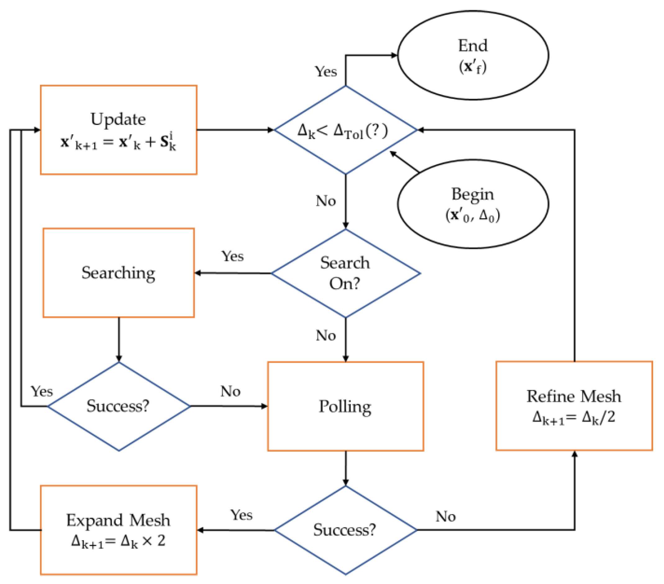
3.5.3. Pattern Search Flowchart

The pattern search method generates neighborhood points, referred to as a mesh, which have a regularized pattern near the initial point. Enabling the search method allows for determining which points reduce the value of the objective function, as shown in Figure 9. If the search method finds a new point that can improve the value of the objective function, this point can be the current point. Polling is performed when the search method does not reduce the value of the objective function. For polling, the current size of the mesh (${∆}_{\mathrm{k}}$) is expanded when there is a point that reduces the objective function value, whereas the size of the mesh is refined if not. Even if polling is performed, if the value of the objective function does not decrease, the size of the mesh continues to be contracted. As this process continues, if the size of the mesh is within the given tolerance condition, polling is stopped, and the current point becomes the global solution of this problem. The multiplying factor for the mesh size is 2, and the mesh tolerance is 1 × 10⁻⁶.

3.6. Optimization Problem Formulation

The optimization problem for the trajectory design of the Mars explorer can be formulated as Equation (10). As there is a strong operational constraint that the entire phase of MOI should remain in contact with our KDSA, the penalty term (${\mathrm{K}}_1$) is augmented.

$$\begin{array}{c}\mathrm{J}=\min \mathrm{f}\left({\mathrm{x}}^{\prime }\right)=‖∆{\mathrm{V}}_{\mathrm{T}\mathrm{M}\mathrm{I}}‖+‖∆{\mathrm{V}}_{\mathrm{M}\mathrm{O}\mathrm{I}}‖+{\mathrm{K}}_1\\ \mathrm{S}\mathrm{u}\mathrm{b}\mathrm{j}\mathrm{e}\mathrm{c}\mathrm{t} \mathrm{t}\mathrm{o}\hspace{1em}{\mathrm{c}\mathrm{e}\mathrm{q}}_1:\mathbf{f}\left(\mathbf{x}\right)-{\left[\begin{array}{ccc}{\mathsf{\delta }}_{\mathrm{D}\mathrm{e}\mathrm{p}}& {\mathsf{\alpha }}_{\mathrm{D}\mathrm{e}\mathrm{p}}& {\mathrm{C}}_3\end{array}\right]}^{\mathrm{T}}=0,{\mathrm{t}}_{\mathrm{L}\mathrm{a}\mathrm{u}\mathrm{n}\mathrm{c}\mathrm{h}}\le \mathrm{t}\le {\mathrm{t}}_{\mathrm{T}\mathrm{L}\mathrm{I}}\\ {\mathrm{c}\mathrm{e}\mathrm{q}}_2:\mathbf{f}\left(\mathbf{x}\right)-{\left[\begin{array}{ccc}{\mathrm{B}}_{\mathrm{t}}& {\mathrm{B}}_{\mathrm{t}}& {\mathrm{t}}_{\mathrm{A}\mathrm{r}\mathrm{r}\mathrm{i}\mathrm{v}\mathrm{a}\mathrm{l}}\end{array}\right]}^{\mathrm{T}}=0,{\mathrm{t}}_{\mathrm{L}\mathrm{a}\mathrm{u}\mathrm{n}\mathrm{c}\mathrm{h}}\le \mathrm{t}\le {\mathrm{t}}_{\mathrm{A}\mathrm{r}\mathrm{r}\mathrm{i}\mathrm{v}\mathrm{a}\mathrm{l}}\hspace{1em}\hspace{1em}\\ {\mathrm{c}\mathrm{e}\mathrm{q}}_3:\mathbf{f}\left(\mathbf{x}\right)-{\left[\begin{array}{ccc}{\mathrm{i}}_{\mathrm{M}}& {\mathrm{h}}_{\mathrm{M}}& {\mathrm{t}}_{\mathrm{A}\mathrm{r}\mathrm{r}\mathrm{i}\mathrm{v}\mathrm{a}\mathrm{l}}\end{array}\right]}^{\mathrm{T}}=0,{\mathrm{t}}_{\mathrm{L}\mathrm{a}\mathrm{u}\mathrm{n}\mathrm{c}\mathrm{h}}\le \mathrm{t}\le {\mathrm{t}}_{\mathrm{A}\mathrm{r}\mathrm{r}\mathrm{i}\mathrm{v}\mathrm{a}\mathrm{l}}\\ {\mathrm{c}\mathrm{e}\mathrm{q}}_4:\mathbf{f}\left(\mathbf{x}\right)-{\mathrm{T}}_{\mathrm{M}}\left(35 \mathrm{h}\right)=0,\hspace{1em}{\mathrm{t}}_{\mathrm{M}\mathrm{O}\mathrm{I}}^{\mathrm{S}\mathrm{t}\mathrm{a}\mathrm{r}\mathrm{t}}\le \mathrm{t}\le {\mathrm{t}}_{\mathrm{M}\mathrm{O}\mathrm{I}}^{\mathrm{S}\mathrm{t}\mathrm{o}\mathrm{p}}\\ {\mathrm{c}\mathrm{e}\mathrm{q}}_5:{\mathbf{f}\left(\mathbf{x}\right)-\mathrm{t}}_{\mathrm{L}\mathrm{a}\mathrm{u}\mathrm{n}\mathrm{c}\mathrm{h}}-{\mathrm{x}}^{\prime }=0,\hspace{1em}{\mathrm{t}}_{\mathrm{L}\mathrm{a}\mathrm{u}\mathrm{n}\mathrm{c}\mathrm{h}}\le \mathrm{t}\le {\mathrm{t}}_{\mathrm{A}\mathrm{r}\mathrm{r}\mathrm{i}\mathrm{v}\mathrm{a}\mathrm{l}}\\ {\mathrm{b}}_1:{{\mathrm{x}}^{\prime }}_{\mathrm{l}\mathrm{b}}({{\mathrm{x}}^{\prime }}_0-10\mathrm{d}\mathrm{a}\mathrm{y})\le {\mathrm{x}}^{\prime }\le {{\mathrm{x}}^{\prime }}_{\mathrm{u}\mathrm{b}}({{\mathrm{x}}^{\prime }}_0+10\mathrm{d}\mathrm{a}\mathrm{y})\\ {\mathrm{c}}_1\left(\mathrm{T}\mathrm{O}\mathrm{F}\right):\left[{\mathrm{t}}_{\mathrm{M}\mathrm{O}\mathrm{I}}^{\mathrm{S}\mathrm{t}\mathrm{a}\mathrm{r}\mathrm{t}},{\mathrm{t}}_{\mathrm{M}\mathrm{O}\mathrm{I}}^{\mathrm{S}\mathrm{t}\mathrm{o}\mathrm{p}}\right]=∆{\mathrm{t}}_{\mathrm{M}\mathrm{O}\mathrm{I}}\subset \left[{\mathrm{t}}_{\mathrm{K}\mathrm{D}\mathrm{S}\mathrm{A}-\mathrm{E}\mathrm{x}\mathrm{p}.}^{\mathrm{S}\mathrm{t}\mathrm{a}\mathrm{r}\mathrm{t}},{\mathrm{t}}_{\mathrm{K}\mathrm{D}\mathrm{S}\mathrm{A}-\mathrm{E}\mathrm{x}\mathrm{p}.}^{\mathrm{S}\mathrm{t}\mathrm{o}\mathrm{p}}\right]=∆{\mathrm{t}}_{\mathrm{K}\mathrm{D}\mathrm{S}\mathrm{A}-\mathrm{E}\mathrm{x}\mathrm{p}.}\\ {\mathrm{K}}_1=0 \mathrm{i}\mathrm{f}∆{\mathrm{t}}_{\mathrm{M}\mathrm{O}\mathrm{I}}\subset ∆{\mathrm{t}}_{\mathrm{K}\mathrm{D}\mathrm{S}\mathrm{A}-\mathrm{E}\mathrm{x}\mathrm{p}.},\mathrm{O}\mathrm{t}\mathrm{h}\mathrm{e}\mathrm{r}\mathrm{w}\mathrm{i}\mathrm{s}\mathrm{e},0<{\mathrm{K}}_1\le 50\end{array}$$

(10)

There are several general equality constraints ($\mathbf{c}\mathbf{e}\mathbf{q}\left(\mathbf{x}\right)=0)$. In order to approach Mars from the launch site, three equality constraints (${\mathrm{c}\mathrm{e}\mathrm{q}}_1~{\mathrm{c}\mathrm{e}\mathrm{q}}_3$) are necessary even if these control variables ($\mathbf{x}=[{\mathrm{t}}_{\mathrm{L}\mathrm{a}\mathrm{u}\mathrm{n}\mathrm{c}\mathrm{h}}$, $∆{\mathrm{t}}_{\mathrm{C}\mathrm{o}\mathrm{a}\mathrm{s}\mathrm{t}},∆{\mathrm{V}}_{\mathrm{T}\mathrm{M}\mathrm{I}}]$) are also used to meet the ${\mathrm{t}}_{\mathrm{A}\mathrm{r}\mathrm{r}\mathrm{i}\mathrm{v}\mathrm{a}\mathrm{l}}$, ${\mathrm{i}}_{\mathrm{M}}$(90$°$) and ${\mathrm{h}}_{\mathrm{M}}$(425 km) in the “Mars approach” problem in Table 4. ${\mathrm{C}\mathrm{e}\mathrm{q}}_4$ is required for capturing the Mars orbit ($\mathrm{x}=[∆{\mathrm{t}}_{\mathrm{M}\mathrm{O}\mathrm{I}}]$) and the global state variable (${\mathrm{x}}^{\prime }$), ${\mathrm{c}\mathrm{e}\mathrm{q}}_5$, can determine the arrival time at Mars. The equality constraint can only deal with the differential corrections process in Section 3.4, but the pattern search method can control the bound constraint ($\mathrm{l}\mathrm{b}\left({{\mathrm{x}}^{\prime }}_{\mathrm{l}\mathrm{b}}\right)\le \left({\mathrm{x}}^{\prime }\right)\le \mathrm{u}\mathrm{b}\left({{\mathrm{x}}^{\prime }}_{\mathrm{u}\mathrm{b}}\right)$) and inequality constraint ($\mathrm{c}\left({\mathrm{x}}^{\prime }\right)\le 0)$. Taking into account a reasonable search boundary for the TOF, the bound constraint is set as the lower (${{\mathrm{x}}^{\prime }}_{\mathrm{l}}$) and upper (${{\mathrm{x}}^{\prime }}_{\mathrm{u}}$) bounds remain within a 10-day range of the initial condition. According to Figure 5, when the Earth departure date is 19 December 2030, the appropriate arrival date is around September 27, 2031, so that the required TOF from Earth departure in this case is approximately 282.33 days. Therefore, we set the initial value of TOF (${\mathrm{x}}_0^{\prime }$) to 282.33 and let the pattern search method find the optimal TOF that satisfies the operational constraints and minimizes the required $∆\mathrm{V}$. In order to have a minimum value of the objective function, the entire burn duration for MOI $[{\mathrm{t}}_{\mathrm{M}\mathrm{O}\mathrm{I}}^{\mathrm{S}\mathrm{t}\mathrm{a}\mathrm{r}\mathrm{t}},{\mathrm{t}}_{\mathrm{M}\mathrm{O}\mathrm{I}}^{\mathrm{S}\mathrm{t}\mathrm{o}\mathrm{p}}]$ should be within the coverage window between KDSA and the Mars explorer $[{\mathrm{t}}_{\mathrm{K}\mathrm{D}\mathrm{S}\mathrm{A}-\mathrm{E}\mathrm{x}\mathrm{p}.}^{\mathrm{S}\mathrm{t}\mathrm{a}\mathrm{r}\mathrm{t}},{\mathrm{t}}_{\mathrm{K}\mathrm{D}\mathrm{S}\mathrm{A}-\mathrm{E}\mathrm{x}\mathrm{p}.}^{\mathrm{S}\mathrm{t}\mathrm{o}\mathrm{p}}]$. It can be regarded as an inequality constraint so that if the burn duration for MOI is beyond the coverage window or is partially covered, ${\mathrm{K}}_1$ would be less than 50, as shown in the inequality constraint in Equation (10). The reason for using 50 for k1, which is about 10 times larger than the $∆\mathrm{V}$ required for a Mars mission, is to make it easier to verify that the constraints are satisfied as the optimization progresses.

Figure 10 shows the overall process to find a global optimal solution. In the global optimal process, when executing the targeting problem (sub-function process), the differential corrections process is employed to solve the four targeting problems described in Table 4. Once $∆{\mathrm{V}}_{\mathrm{T}\mathrm{M}\mathrm{I}}$, $∆{\mathrm{V}}_{\mathrm{M}\mathrm{O}\mathrm{I}}$, ${\mathrm{t}}_{\mathrm{M}\mathrm{O}\mathrm{I}}^{\mathrm{S}\mathrm{t}\mathrm{a}\mathrm{r}\mathrm{t}}$, ${\mathrm{t}}_{\mathrm{M}\mathrm{O}\mathrm{I}}^{\mathrm{S}\mathrm{t}\mathrm{o}\mathrm{p}}$, ${\mathrm{t}}_{\mathrm{K}\mathrm{D}\mathrm{S}\mathrm{A}-\mathrm{E}\mathrm{x}\mathrm{p}.}^{\mathrm{S}\mathrm{t}\mathrm{a}\mathrm{r}\mathrm{t}}$ and ${\mathrm{t}}_{\mathrm{K}\mathrm{D}\mathrm{S}\mathrm{A}-\mathrm{E}\mathrm{x}\mathrm{p}.}^{\mathrm{S}\mathrm{t}\mathrm{o}\mathrm{p}}$ are obtained, the pattern search utilizes them to compute the value of the objective function, as shown in Equation (10), and proceeds to find the global solution following the steps outlined in Figure 9. In other words, the pattern of the global state variable (TOF) is continuously expanded and contracted, causing the Mars arrival time to continually change so that the differential corrections process is then iteratively performed based on these changes. If the value of the objective function does not decrease, and the mesh size is below the tolerance threshold (${∆}_{\mathrm{T}\mathrm{o}\mathrm{l}}=$1 × 10⁻⁶), the global process is terminated.

4. Numerical Simulation Results and Discussion

4.1. Results of Global Optimization Problem

Figure 11 illustrates the process of optimizing the trajectory of the ascending departure on 19 December 2030, using the pattern search method. A pattern is employed to generate a global state variable (TOF) that deviates significantly from the initial value, and then it is used to adjust the arrival time at Mars. Subsequently, a sub-function (differential corrections process in Table 4) call was executed to ensure that the explorer arrives at Mars at the specified time and meets the orbit elements for MOI. Based on these results, the process of gradually narrowing down the range of TOF is depicted in detail in the upper graph of Figure 11a, while confirming whether the value of the objective function decreases. In the lower graph of Figure 11a, there are many points where the value of the objective function exceeds 50. The reason for this is that ${\mathrm{K}}_1$ in Equation (10) has reached 50, which implies that the MOI coverage is beyond the monitoring capabilities of KDSA.

The process of finding the minimum value of the objective function using the pattern search method is shown in the upper graph of Figure 11b. Successful searches were conducted at the 2nd, 4th and 8th iteration, while a successful poll was performed at the 14th iteration, leading to an update of a new state that reduced the value of the objective function. The average number of calls of the sub-function was about 4 until the new state was updated or the mesh size was changed to the condition of asking if the pattern search can be terminated. During a total of 20 iterations of the pattern search for global optimization, the sub-function executed a total of 74 iterations. The simulation results not only provide a robustness of the convergence characteristics of the pattern search method, but also demonstrate its computational efficiency, as evidenced by the relatively low frequency of main and sub-function calls.

Based on the confirmation of the practical applicability of the pattern search method in designing optimal trajectories for Mars exploration, the trajectories for both the ascending and descending departure were designed within a 15-day launch period, considering the possibility of launching twice a day. The launch occurred at the Naro Space Center, and the KSLV-II puts the payload into the parking orbit with an altitude of 300 km and an inclination of 80° for an ascent duration of 870 s. The launch epoch and TMI epoch determined the ascending and descending departure, as shown in Figure 12a. In order to send the explorer from Earth’s northern hemisphere (ascending departure) to Mars, the launch epoch should be around 00:00 (UTC) and the required coast duration was approximately 50 min so that the TMI maneuver is performed at approximately launch + 65 min. On the other hand, for the descending departure, the launch epoch should be around 12:00 (UTC) and the required coast duration was approximately 100 min so that the TMI maneuver is executed at approximately launch + 120 min. Furthermore, it was observed that with each day of launch delay, the launch epoch advanced by approximately 3 min.

Figure 12b illustrates the variation in ${\mathrm{C}}_3$, DLA and RLA over a 15-day launch period. Firstly, as the launch date was delayed, ${\mathrm{C}}_3$ gradually decreased, leading to a slight reduction in the required TMI ∆V. To reach Mars, the inclination of the parking orbit must be greater than the DLA [3]. As the launch date was postponed, the DLA slightly increased, but it remained below 80°, enabling Mars access during all the periods. The RLA directly affects the launch epoch [34], and the reason the launch epoch in Figure 12a did not significantly change over the 15-day period is that the RLA only varied by 3° during that period.

The converged TOF and ${\mathrm{V}}_{\mathrm{\infty }}$ for this period is shown in Figure 13a. The TOF initially started at 282.33 days, but through optimization and while satisfying the operational and bound constraints, it converged to a value within approximately one day of the initial value. In the case of ${\mathrm{V}}_{\mathrm{\infty }}$, it gradually increased, unlike ${\mathrm{C}}_3$, and it can be observed that it was slightly lower for the ascending departure than for the descending departure. Reflecting these results, the trends of TMI ∆V and MOI ∆V are displayed in Figure 13b. It can be observed that TMI ∆V (influenced by ${\mathrm{C}}_3$) increased as the launch date was delayed, whereas MOI ∆V (affected by ${\mathrm{V}}_{\mathrm{\infty }}$) gradually decreased. Above all, it was evident that the ascending departure requires a generally lower ∆V compared to the descending departure. When the explorer traveled from Earth to Mars for approximately 282 days, Mars was situated in the southern hemisphere of Earth and the geocentric latitude changed from 6° S to 25° S. A detailed analysis of the latitude where TMI is executed during the 15-day launch period confirmed that the TMI latitude of the ascending departure changed from 21.3° N (Figure 6) to 12.3° N, and the TMI latitude of the descending departure changed from 44.2° S to 49.7° S. The reason TMI was conducted at such latitudes is that Mars was located in the southern hemisphere of Earth. Due to the highly inclined transfer orbit and latitude variations of Mars relative to Earth’s equatorial plane, it is estimated that the ascending departure has a lower ∆V than the descending departure.

Figure 14a illustrates the overall trend of the total ∆V according to the Earth departure and Mars arrival dates. The ascending departure required slightly less ∆V than the descending departure on the order of 10 m/s, and the date requiring the minimum ∆V for both departures was determined to be 26 September 2030; however, as the launch date was delayed within the 15-day launch period, the TMI ∆V decreased while the MOI ∆V increased, as shown in Figure 13b. Therefore, when estimating the mass of the upper stage of the launch vehicle and the Mars explorer, it is necessary to consider this aspect. The detailed processes to estimate the mass are described in Section 4.2.

Communication between an explorer, including those exploring the Moon and Mars, and the ground-based deep space antennas is typically limited to around 8 h a day due to the Earth’s rotation. Therefore, as shown in Figure 14b, it can be observed that KDSA, with a 5° elevation angle constraint, and the Mars explorer were capable of approximately 8 h of coverage per day, even if the arrival date on Mars of the explorer varied. Most importantly, as the approximately 13 min of the MOI burn duration (${∆\mathrm{t}}_{\mathrm{M}\mathrm{O}\mathrm{I}}$) can always be within the contact duration between KDSA and explorer (${∆\mathrm{t}}_{\mathrm{K}\mathrm{D}\mathrm{S}\mathrm{A}-\mathrm{E}\mathrm{X}\mathrm{P}}$) regardless of the arrival date, it can be concluded that the global optimization using the pattern search method definitively satisfies the operational constraint (by making ${\mathrm{K}}_1$ equal to 0). The optimization results of the trajectory design are shown in detail in

Table A1. Optimization results of ascending departure for 15-day launch period (Part 1).

No.	${\mathbf{t}}_{\mathbf{L}\mathbf{a}\mathbf{u}\mathbf{n}\mathbf{c}\mathbf{h}}$ (UTC)	${∆\mathbf{t}}_{\mathbf{C}\mathbf{o}\mathbf{a}\mathbf{s}\mathbf{t}}$ (min)	${\mathbf{t}}_{\mathbf{T}\mathbf{M}\mathbf{I}}$ (UTC)	${∆\mathbf{V}}_{\mathbf{T}\mathbf{M}\mathbf{I}}$ (km/s)	${\mathbf{C}}_3$ (km2/s2)	${\mathsf{\alpha }}_{\mathbf{D}\mathbf{e}\mathbf{p}}$ (deg)	${\mathsf{\delta }}_{\mathbf{D}\mathbf{e}\mathbf{p}}$ (deg)
1	19 Dec, 2030 00:30:55	52.72	19 Dec, 2030 01:33:38	3.718	11.610	227.94	11.44
2	20 Dec, 2030 00:28:42	52.53	20 Dec, 2030 01:31:14	3.711	11.442	228.28	11.97
3	21 Dec, 2030 00:26:17	52.35	21 Dec, 2030 01:28:38	3.704	11.279	228.56	12.47
4	22 Dec, 2030 00:23:57	52.11	22 Dec, 2030 01:26:04	3.698	11.145	228.82	13.27
5	23 Dec, 2030 00:21:33	51.93	23 Dec, 2030 01:23:29	3.692	11.007	229.11	13.78
6	24 Dec, 2030 00:19:08	51.75	24 Dec, 2030 01:20:53	3.686	10.879	229.39	14.32
7	25 Dec, 2030 00:16:38	51.58	25 Dec, 2030 01:18:13	3.681	10.760	229.65	14.85
8	26 Dec, 2030 00:14:04	51.41	26 Dec, 2030 01:15:29	3.676	10.652	229.89	15.38
9	27 Dec, 2030 00:11:26	51.24	27 Dec, 2030 01:12:40	3.672	10.556	230.12	15.92
10	28 Dec, 2030 00:08:44	51.07	28 Dec, 2030 01:09:49	3.668	10.470	230.33	16.46
11	29 Dec, 2030 00:06:10	50.83	29 Dec, 2030 01:07:00	3.666	10.434	230.49	17.39
12	30 Dec, 2030 00:03:24	50.67	30 Dec, 2030 01:04:04	3.663	10.373	230.68	17.93
13	31 Dec, 2030 00:00:36	50.51	31 Dec, 2030 01:01:06	3.661	10.322	230.86	18.48
14	31 Dec, 2030 23:57:47	50.36	01 Jan, 2031 00:58:08	3.659	10.279	231.03	19.01
15	01 Jan, 2031 23:54:44	50.31	02 Jan, 2031 00:55:03	3.655	10.192	231.24	19.07

,

Table A2. Optimization results of ascending departure for 15-day launch period (Part 2).

No.	$\mathbf{TOF}({\mathbf{x}}^{\prime })$ (Days)	${{\mathbf{x}}^{\prime }}_0$ (Days)	${\mathbf{t}}_{\mathbf{A}\mathbf{r}\mathbf{r}\mathbf{i}\mathbf{v}\mathbf{a}\mathbf{l}}$ (UTC)	${∆\mathbf{t}}_{\mathbf{M}\mathbf{O}\mathbf{I}}$ (min)	${∆\mathbf{V}}_{\mathbf{M}\mathbf{O}\mathbf{I}}$ (km/s)	${\mathbf{V}}_{\mathbf{\infty }}$ (km/s)	${\mathsf{\alpha }}_{\mathbf{A}\mathbf{r}\mathbf{r}}$ (deg)	${\mathsf{\delta }}_{\mathbf{A}\mathbf{r}\mathbf{r}}$ (deg)
1	283.22	282.33	28 Sep, 2031 05:15:55	12.85	1.322	3.448	0.58	−29.88
2	283.19	282.33	29 Sep, 2031 04:27:31	12.87	1.323	3.450	0.60	−30.28
3	283.18	282.33	30 Sep, 2031 04:14:42	12.88	1.325	3.454	0.61	−30.67
4	282.30	282.33	30 Sep, 2031 07:09:39	12.90	1.327	3.457	1.12	−31.09
5	282.26	282.33	01 Oct, 2031 06:12:44	12.92	1.330	3.461	1.14	−31.51
6	282.18	282.33	02 Oct, 2031 04:13:11	12.94	1.333	3.467	1.18	−31.92
7	282.18	282.33	03 Oct, 2031 04:12:28	12.97	1.337	3.473	1.17	−32.33
8	282.18	282.33	04 Oct, 2031 04:13:11	13.01	1.341	3.480	1.16	−32.75
9	282.17	282.33	05 Oct, 2031 04:10:20	13.04	1.346	3.489	1.14	−33.16
10	282.18	282.33	06 Oct, 2031 04:20:18	13.09	1.352	3.498	1.13	−33.57
11	281.41	282.33	06 Oct, 2031 09:48:56	13.12	1.357	3.505	1.56	−34.07
12	281.43	282.33	07 Oct, 2031 10:18:05	13.17	1.363	3.516	1.54	−34.49
13	281.43	282.33	08 Oct, 2031 10:23:04	13.23	1.370	3.527	1.52	−34.91
14	281.47	282.33	09 Oct, 2031 11:14:18	13.29	1.378	3.540	1.49	−35.32
15	282.31	282.33	11 Oct, 2031 07:21:01	13.37	1.389	3.557	0.99	−35.58

,

Table A3. Optimization results of descending departure for 15-day launch period (Part 1).

No.	${\mathbf{t}}_{\mathbf{L}\mathbf{a}\mathbf{u}\mathbf{n}\mathbf{c}\mathbf{h}}$ (UTC)	${∆\mathbf{t}}_{\mathbf{C}\mathbf{o}\mathbf{a}\mathbf{s}\mathbf{t}}$ (min)	${\mathbf{t}}_{\mathbf{T}\mathbf{M}\mathbf{I}}$ (UTC)	${∆\mathbf{V}}_{\mathbf{T}\mathbf{M}\mathbf{I}}$ (km/s)	${\mathbf{C}}_3$ (km2/s2)	${\mathsf{\alpha }}_{\mathbf{D}\mathbf{e}\mathbf{p}}$ (deg)	${\mathsf{\delta }}_{\mathbf{D}\mathbf{e}\mathbf{p}}$ (deg)
1	18 Dec, 2030 12:16:34	103.69	18 Dec, 2030 14:10:15	3.728	11.736	227.80	11.19
2	19 Dec, 2030 12:13:45	103.78	19 Dec, 2030 14:07:32	3.721	11.569	228.18	11.73
3	20 Dec, 2030 12:10:12	103.95	20 Dec, 2030 14:04:09	3.715	11.416	228.44	12.59
4	21 Dec, 2030 12:06:53	104.03	21 Dec, 2030 14:00:55	3.708	11.258	228.69	13.08
5	22 Dec, 2030 12:03:43	104.11	22 Dec, 2030 13:57:49	3.702	11.115	228.97	13.56
6	23 Dec, 2030 12:00:36	104.19	23 Dec, 2030 13:54:47	3.696	10.982	229.27	14.04
7	24 Dec, 2030 11:57:25	104.27	24 Dec, 2030 13:51:41	3.691	10.859	229.55	14.54
8	25 Dec, 2030 11:54:07	104.37	25 Dec, 2030 13:48:29	3.686	10.745	229.81	15.07
9	26 Dec, 2030 11:50:44	104.47	26 Dec, 2030 13:45:12	3.681	10.643	230.05	15.59
10	27 Dec, 2030 11:47:16	104.58	27 Dec, 2030 13:41:50	3.677	10.552	230.27	16.12
11	28 Dec, 2030 11:43:44	104.69	28 Dec, 2030 13:38:25	3.674	10.472	230.47	16.66
12	29 Dec, 2030 11:40:11	104.80	29 Dec, 2030 13:34:59	3.671	10.401	230.67	17.17
13	30 Dec, 2030 11:36:36	104.91	30 Dec, 2030 13:31:30	3.668	10.341	230.85	17.69
14	31 Dec, 2030 11:32:59	105.02	31 Dec, 2030 13:28:00	3.666	10.290	231.04	18.21
15	01 Jan, 2031 11:29:24	105.13	01 Jan, 2031 13:24:32	3.664	10.244	231.22	18.68

and

Table A4. Optimization results of descending departure for 15-day launch period (Part 2).

No.	$\mathbf{TOF}({\mathbf{x}}^{\prime })$ (Days)	${{\mathbf{x}}^{\prime }}_0$ (Days)	${\mathbf{t}}_{\mathbf{A}\mathbf{r}\mathbf{r}\mathbf{i}\mathbf{v}\mathbf{a}\mathbf{l}}$ (UTC)	${∆\mathbf{t}}_{\mathbf{M}\mathbf{O}\mathbf{I}}$ (min)	${∆\mathbf{V}}_{\mathbf{M}\mathbf{O}\mathbf{I}}$ (km/s)	${\mathbf{V}}_{\mathbf{\infty }}$ (km/s)	${\mathsf{\alpha }}_{\mathbf{A}\mathbf{r}\mathbf{r}}$ (deg)	${\mathsf{\delta }}_{\mathbf{A}\mathbf{r}\mathbf{r}}$ (deg)
1	283.19	282.33	28 Sep, 2031 04:37:10	12.86	1.323	3.450	0.33	−29.85
2	283.18	282.33	29 Sep, 2031 04:16:16	12.88	1.324	3.452	0.34	−30.24
3	282.26	282.33	29 Sep, 2031 06:19:43	12.89	1.326	3.455	0.87	−30.64
4	282.24	282.33	30 Sep, 2031 05:47:54	12.90	1.328	3.459	0.89	−31.05
5	282.18	282.33	01 Oct, 2031 04:16:25	12.92	1.331	3.463	0.92	−31.45
6	282.18	282.33	02 Oct, 2031 04:12:26	12.95	1.334	3.469	0.92	−31.86
7	282.18	282.33	03 Oct, 2031 04:12:26	12.98	1.338	3.475	0.91	−32.27
8	282.17	282.33	04 Oct, 2031 04:11:56	13.01	1.342	3.482	0.90	−32.68
9	282.17	282.33	05 Oct, 2031 04:10:57	13.05	1.347	3.490	0.89	−33.08
10	282.18	282.33	06 Oct, 2031 04:12:26	13.09	1.353	3.499	0.87	−33.49
11	282.17	282.33	07 Oct, 2031 04:11:56	13.14	1.359	3.509	0.86	−33.89
12	282.21	282.33	08 Oct, 2031 05:00:10	13.19	1.366	3.520	0.83	−34.29
13	282.23	282.33	09 Oct, 2031 05:28:01	13.25	1.373	3.531	0.81	−34.69
14	282.24	282.33	10 Oct, 2031 05:47:55	13.31	1.381	3.544	0.79	−35.09
15	282.33	282.33	11 Oct, 2031 07:55:12	13.37	1.390	3.558	0.73	−35.47

.

4.2. Mass Estimation of the Upper Stage and the Mars Explorer

Even though the lowest total ∆V is required when departing Earth on 26 September 2030, the worst-case TMI ∆V and MOI ∆V must be applied when estimating the mass of the upper stage and the Mars explorer from an overall system design perspective due to uncertainty regarding the actual launch date. For MAVEN, there was a 20-day nominal launch period starting from 18 November 2013. The ${\mathrm{C}}_3$ decreased gradually from 12.23 to 9.30 km²/s², but the actual launch took place on the largest ${\mathrm{C}}_3$ date on 18 November 2013 [3]. Launching on the first day of the launch period can be interpreted as a result of system design that allows the upper stage to handle even the highest ${\mathrm{C}}_3$.

KSLV-II is able to deliver a payload ($m_0^{Payload}$) of 2600 kg, including both the upper stage and Mars explorer, into the parking orbit, and the maximum ${\mathrm{C}}_3$ occurred for the descending departure on Dec 18, 2030. The maximum propellant mass of the upper stage ($m_p^{UpperStage}$) calculated by Equation (11) is 1906.7 kg [35] based on $I_{sp}$ (287.5 s) of the upper stage [20].

$$m_p^{UpperStage}=m_0^{Payload}\left(1-e^{\frac{-{∆V}_{TMI}}{I_{sp}·g_0}}\right)$$

(11)

The final (dry) mass of the upper stage ($m_f^{UpperStage})$ calculated by Equation (12) is 344.4 kg when the structural mass ratio (MR) of the upper stage is 0.153 [15]. According to the results of Equations (11) and (12), the maximum wet mass of the upper stage ($m_0^{UpperStage}$) is 2251.1 kg, and the available wet mass of the Mars explorer can be 348.9 kg.

$$m_f^{UpperStage}=m_p^{UpperStage}\left(\frac{\mathit{M}\mathit{R}}{1-\mathit{M}\mathit{R}}\right)$$

(12)

Since the mass of the explorer that can be sent to Mars has been determined, it is necessary to allocate the required ∆V in detail to estimate the mass of scientific payloads and structures of the explorer. First, similar to the TMI ∆V, the explorer should consider the highest ${\mathrm{V}}_{\mathrm{\infty }}$ when arriving at Mars on 11 October 2031, because the exact launch date within the 15-day launch period is unknown. Secondly, we plan for four to five TCMs during the Mars transfer phase so that we can allocate the TCM ∆V budget (approximately 40 m/s) from the MRO [2]. Thirdly, the current orbit period (35 h) needs to be reduced to within 2 h for science missions. To achieve this, we assume the use of aerobraking over approximately 6 months and we allocate 50 m/s to decrease the orbital period using Mars’s atmosphere [27]. In addition, orbit maintenance and attitude control and margins are allocated based upon the experience of the previous mission;

Table 5. ∆V allocations for Mars explorer.

Event	Translational ∆V
TCM	40 m/s
MOI	1390 m/s
Braking maneuver	50 m/s
Orbit maintenance	20 m/s
Attitude control	66 m/s
Margin	50 m/s
Totals	1616 m/s

shows a list of the ∆V allocations [2,3,36]. The propellant mass of the Mars explorer calculated by Equation (11) with the $I_{sp}$ value of the green hypergolic propulsion system (306.5 s) is 145.0 kg. As a result, the dry mass of the Mars explorer, including the payload, structure, electronics and propulsion system, is finally 203.8 kg.

5. Conclusions

By setting the Mars landing mission as a national agenda for the year 2045, South Korea is accelerating its efforts in deep space exploration. In this context, we have designed optimized trajectories departing from Earth on December 2030 utilizing domestic infrastructure, such as the Naro Space Center, KSLV-II, KDSA and an eco-friendly hypergolic propulsion system, to assess the feasibility of Mars exploration. We established scenarios for both ascending and descending departures and performed global optimization using the pattern search method to minimize the required ∆V while satisfying operational constraints to maintain coverage of the complete MOI duration. As a result, the convergence characteristics of the pattern search method were quite evident, and it was observed that optimal solutions were well derived while satisfying the nonlinear constraints. Furthermore, notably, it was confirmed that the ascending departures showed an improvement on the order of 10 m/s compared to the descending departures. Based on the application of realistic launch conditions, the derived mass of the upper stage resulted in an achievable wet mass and dry mass for the Mars explorer of approximately 348.9 kg and 203.8 kg, respectively. This study is expected to provide significant assistance in the future for the selection and allocation of specific scientific payloads and their weights, given that Mars exploration is sufficiently feasible with the resources available to South Korea.

References

1. South Korean Ministry of Science and ICT. Fourth Space Development Promotion Basic Plan. Available online: https://english.khan.co.kr/khan_art_view.html?artid=202212221752047&code=710100 (accessed on 22 December 2022).
2. Halsell, C.A.; Bowes, A.L.; Johnston, M.D.; Lyons, D.T.; Lock, R.E.; Xaypraseuth, P.; Bhaskaran, S.; Highsmith, D.E.; Jah, M.K. Trajectory design for the Mars reconnaissance orbiter mission. In Proceedings of the AAS/AIAA Space Flight Mechanics Meeting, Ponce, Puerto Rico, USA, 9–13 February 2003. [Google Scholar]
3. Folta, D.; Demcak, S.; Young, B.; Berry, K. Transfer trajectory design for the Mars atmosphere and volatile evolution (MAVEN) mission. In Proceedings of the AAS/AIAA Space Flight Mechanics Meeting, Kauai, HI, USA, 10–14 February 2013. [Google Scholar]
4. Schmidt, R. Mars express-ESA’s first mission to planet Mars. Acta Astronaut. 2003, 52, 197–202. [Google Scholar] [CrossRef]
5. Long, S.; Lyons, D.; Guinn, J.; Lock, R. ExoMars/TGO Science Orbit Design. In Proceedings of the AAS/AIAA Astrodynamics Specialist Conference, Minneapolis, MN, USA, 13–16 August 2012. [Google Scholar]
6. Sundararajan, V. Mangalyaan–Overview and technical architecture of Inian’s first interplanetary mission to Mars. In Proceedings of the AIAA Space 2013 Conference and Exposition, San Diego, CA, USA, 10–12 September 2013. [Google Scholar]
7. Alrais, A.; Bester, M.; Stroozas, B.; Alloghani, M. Emirates Mars mission–Al Amal Overview. In Proceedings of the SpaceOps Conferences, Daejeon, Republic of Korea, 16–20 May 2016. [Google Scholar]
8. Ye, P.; Sun, Z.; Rao, W.; Meng, L. Mission overview and key technologies of the first Mars probe of China. Sci. China Technol. Sci. 2017, 60, 649–657. [Google Scholar] [CrossRef]
9. Gooding, R.H. A procedure for the solution of Lambert’s orbital boundary-value problem. Celest. Mech. Dyn. Astron. 1990, 48, 145–165. [Google Scholar] [CrossRef]
10. Sellers, J.J. Understanding Space: An Introduction to Astronautics, 2nd ed.; Mc Graw Hill: New York, NY, USA, 2005; pp. 227–248. [Google Scholar]
11. Abdelkhalik, O.; Mortari, D. N-Impulse Orbit Transfer Using Genetic Algorithms. J. Spacecr. Rocket. 2007, 44, 456–460. [Google Scholar] [CrossRef]
12. Vasile, M.; Summerer, L.; Pascale, P.D. Design of Earth-Mars transfer trajectories using evolutionary-branching technique. Acta Astronaut. 2005, 56, 705–720. [Google Scholar] [CrossRef]
13. Ellipson, D.H.; Conway, B.A. Analytic Gradient Computation for Bounded-Impulse Trajectory Models Using Two-Sided Shooting. J. Guid. Control. Dyn. 2018, 41, 1449–1462. [Google Scholar] [CrossRef] [PubMed]
14. Miele, A.; Wang, T.; Williams, P.N. Computation of optimal Mars trajectories via combined chemical/electrical propulsion, part 1: Baseline solutions for deep interplanetary space. Acta Astronaut. 2004, 55, 95–107. [Google Scholar] [CrossRef]
15. Gagg Filho, L.A.; da Silva Fernandes, S. Optimal Two-Impulse Interplanetary Trajectories: Earth-Venus and Earth-Mars Missions. Rev. Mex. Astron. Astrofís. 2023, 59, 11–43. [Google Scholar] [CrossRef]
16. Izzo, D.; Sprague, C.; Tailor, D. Machine learning and evolutionary techniques in interplanetary trajectory design. In Modeling and Optimization in Space Engineering; Fasano, G., Pintér, J.D., Eds.; Springer: Berlin, Germany, 2019; pp. 191–210. [Google Scholar]
17. Global Optimization Toolbox User’s Guide. Matlab, R2019a, The Mathworks Inc, Massachusetts. Available online: https://www.mathworks.com/help/gads/ (accessed on 1 March 2019).
18. Kolda, T.G.; Lewis, R.M.; Torczon, V. A Generating Set Direct Search Argumented Lagrangian Algorithm for Optimization with a Combination of General and Linear Constraints; Technical Report, SAND2006-5315; Sandia National Laboratories: California, CA, USA, 2006. [Google Scholar]
19. Choi, S.J.; Song, Y.J.; Bae, J.H.; Kim, E.H.; Ju, G.H. Design and analysis of Korean lunar orbiter mission using direct transfer. J. Korean Soc. Aeronaut. Space Sci. 2013, 41, 1225–1348. [Google Scholar]
20. Korea Advanced Institute of Science and Technology, Feasibility Study for Korean lunar Exploration Project Step 2. Ministry of Science and ICT. Available online: https://scienceon.kisti.re.kr/srch/selectPORSrchReport.do?cn=TRKO201800006037 (accessed on 31 March 2017).
21. Ko, J.; Cho, S.Y. Space Launch vehicle development in Korea aerospace research institute. In Proceedings of the SpaceOps Conferences, Daejeon, Republic of Korea, 16–20 May 2016. [Google Scholar]
22. Kang, H.; Jang, D.; Kwon, S. Demonstration of 500 N scale bipropellant thruster using non-toxic hypergolic fuel and hydrogen peroxide. Aerosp. Sci. Technol. 2016, 49, 209–214. [Google Scholar] [CrossRef]
23. Kang, H.; Kwon, S. Green hypergolic combination: Diethylenetriamine-based fuel and hydrogen peroxide. Acta Astronaut. 2017, 137, 25–30. [Google Scholar] [CrossRef]
24. Kim, Y.R.; Song, Y.J.; Bae, J.H.; Choi, S.W. Observational arc-length effect on orbit determination for KPLO using a sequential estimation technique. J. Astron. Space Sci. 2018, 35, 295–308. [Google Scholar]
25. Laura, M.; Robert, D.F.; Melissa, L.M. Interplanetary Mission Design Handbook: Earth to Mars Mission Opportunities 2026 to 2045; Clenn Research Center: Cleveland, OH, USA, 2010. [Google Scholar]
26. Choi, S.J.; Carrico, J.; Loucks, M.; Lee, H.; Kwon, S. Geostationary Orbit Transfer with Lunar Gravity Assist from Non-equatorial Launch Site. J. Astronaut. Sci. 2021, 68, 1014–1033. [Google Scholar] [CrossRef]
27. Long, S.M.; You, T.H.; Halsell, C.A.; Bhat, R.S.; Demcak, S.W.; Graat, E.J.; Higa, E.S.; Highsmith, D.E.; Mottinger, N.A.; Jah, M.K. Mars Reconnaissance Orbiter Aerobraking Navigation Operation. In Proceedings of the SpaceOps Conferences, Heidelberg, Germany, 12–16 May 2008. [Google Scholar]
28. Berry, M.M.; Coppola, V.T. Integration of orbit trajectories in the presence of multiple full gravitational fields. In Proceedings of the AAS/AIAA Space Flight Mechanics Meeting, Galveston, TX, USA, 27–31 January 2008. [Google Scholar]
29. Cook, G.E. Satellite drag coefficients. Planet. Space Sci. 1965, 10, 929–946. [Google Scholar] [CrossRef]
30. Tolson, R.H.; Lugo, R.A.; Baird, D.T.; Cianciolo, A.D.; Bougher, S.W.; Zurek, R.M. Atmospheric modeling using accelerometer data during Mars Atmosphere and Volatile Evolution (MAVEN) flight operations. In Proceedings of the AAS/AIAA Space Flight Mechanics Meeting, San Antonio, TX, USA, 5–9 February 2017. [Google Scholar]
31. Berry, M.M. Comparisons between Newton-Raphson and Broyden’s methods for trajectory design problems. In Proceedings of the AAS/AIAA Astrodynamics Specialist Conference, Girdwood, AK, USA, 31 July–4 August 2011. [Google Scholar]
32. Ansys Systems Tool Kit/Astrogator, Software Package, Ver. 12.1.0. Available online: https://www.ansys.com/products/missions/ansys-stk (accessed on 13 November 2020).
33. Choi, S.J.; Lee, D.; Kim, I.K.; Kwon, J.W.; Koo, C.H.; Moon, S.; Kim, C.; Min, S.Y.; Rew, D.Y. Trajectory Optimization for a lunar orbiter using a pattern search method. Proc. Inst. Mech. Eng. G J. Aerosp. Eng. 2017, 231, 1325–1337. [Google Scholar] [CrossRef]
34. Loucks, M.; Carrico, J.; Carrico, T.; Deiterich, C. A Comparison of Lunar Landing Trajectory Strategies using Numerical Simulations. In Proceedings of the International Lunar Conference, Toronto, ON, Canada, 18–23 September 2005. [Google Scholar]
35. Sutton, G.P.; Biblarz, O. Rocket Propulsion Elements, 7th ed.; John Wiley & Sons: New York, NY, USA, 2001; pp. 102–106. [Google Scholar]
36. Spencer, D.A.; Tolson, R. Aerobraking cost and risk decisions. J. Spacecr. Rocket. 2007, 42, 1285–1293. [Google Scholar] [CrossRef]
Figure 1. Facilities of Naro Space Center.
Aerospace 10 00827 g001
Figure 2. Schematic of pressure-fed system for the hypergolic thruster.
Aerospace 10 00827 g002
Figure 3. Demonstration of a 500 N-scale green hypergolic thruster with stock 2 fuel and 90 wt.% H2O2 oxidizers.
Aerospace 10 00827 g003
Figure 4. Overview of Korea deep space antenna.
Aerospace 10 00827 g004
Figure 5. The solution to Lambert’s problem based on an approximate 40-day departure and arrival period: (a) Earth departure energy ( C 3 ) and Mars excessive velocity ( V ); (b) declination ( δ D e p ) and right ascension ( α D e p ) of launch asymptote.
Aerospace 10 00827 g005
Figure 6. Ascending Earth departure trajectory (Earth fixed frame); E R = Earth’s radius.
Aerospace 10 00827 g006
Figure 7. Mars transfer trajectory with Earth and Mars orbits (Sun inertial frame); AU = astronomical unit.
Aerospace 10 00827 g007
Figure 8. Mars orbit insertion trajectory (Mars inertial frame); M R = Mars’s radius.
Aerospace 10 00827 g008
Figure 9. Flowchart for the pattern search method.
Aerospace 10 00827 g009
Figure 10. Overall flowchart to calculate global optimal solution.
Aerospace 10 00827 g010
Figure 11. The process of optimizing the trajectory of ascending departure on 19 December 2030, using the pattern search method: (a) TOF and value of objective function in sub-function call (differential corrections process); (b) convergence process of global optimization and the number of sub-function calls per pattern search iteration.
Aerospace 10 00827 g011
Figure 12. Major parameters to depart Earth to travel to Mars: (a) launch and TMI epochs for both ascending and descending departure; (b) C 3 , DLA and RLA.
Aerospace 10 00827 g012
Figure 13. Major parameters to depart Earth and arrive at Mars: (a) converged TOF and V at Mars arrival; (b) TMI and MOI ∆V trend for both ascending and descending departures.
Aerospace 10 00827 g013
Figure 14. (a) Total ∆V with departure and arrival dates for both ascending and descending departures; (b) contact duration between KDSA and Mars explorer ( t K D S A E X P ), and MOI burn duration ( t M O I ) within contact duration for both ascending and descending departures.
Aerospace 10 00827 g014