Article

Numerical Simulation of an Electrothermal Ice Protection System in Anti-Icing and Deicing Mode

by
Lokman Bennani
1,*,†,
Pierre Trontin
2,† and
Emmanuel Radenac
1,†
1
ONERA/DMPE, Université de Toulouse, 31055 Toulouse, France
2
Univ Lyon, Univ Claude Bernard Lyon 1, CNRS, Ecole Centrale de Lyon, INSA Lyon, LMFA, UMR5509, 69622 Villeurbanne, France
*
Author to whom correspondence should be addressed.
These authors contributed equally to this work.
Aerospace 2023, 10(1), 75; https://doi.org/10.3390/aerospace10010075
Submission received: 29 November 2022 / Revised: 19 December 2022 / Accepted: 7 January 2023 / Published: 11 January 2023
(This article belongs to the Special Issue Deicing and Anti-Icing of Aircraft (Volume III))

Abstract

:
The design of efficient thermal ice protection systems is a challenging task as these systems operate in complex environments involving several coupled physical phenomena such as phase change, boundary-layer flow, and heat transfer. Moreover, certification rules are becoming more stringent, and there is a strong incentive for the reduction of fuel consumption. In this context, numerical tools provide a powerful asset during the design phase but also to gain insight into the physical mechanisms at play. This article presents modeling and simulation strategies for thermal ice protection systems. First, the model describing the behavior of the thermal protection system is presented. Second, a model and associated numerical method is presented for unsteady ice accretion. Third, the coupling methodology between the ice accretion solver and the heat conduction solver is described. In the fourth part, different methods to simulate the boundary-layer flow are described. Finally, some relevant examples are presented, both in steady and unsteady configurations.

1. Introduction

In order to comply with more and more stringent certifications and regulations regarding flight safety in icing conditions, aircraft manufacturers design and use ice protection systems. In the context of “more electric” aircraft, electrothermal ice protection systems (ETIPS) are being investigated. This system is composed of heater mats installed within a multi-layered material and can be used in anti-icing or deicing configurations [1,2]. Nowadays, the ETIPS are generally a purely active deicing and anti-icing solution. This is a starting hypothesis of the present article. The combination of ETIPS with an icephobic coating is indeed still little studied, although some recent work shows that it is a valuable field of investigation [3,4] in order to reduce the energy consumption of IPS.
Figure 1 shows the nominal functioning of an ETIPS in deicing mode. The region located at the leading edge is constantly anti-iced and is called the parting strip. In regions other than the parting strip, ice accretion is permitted, and the heaters are activated cyclically. When a heater mat is activated, it melts a part of the ice in contact with the surface, creating a liquid water film and therefore lowering the ability of the ice block to adhere to the surface. The aerodynamic forces are then able to detach the ice block (or part of it) from the surface.
This type of system operates in a complex environment involving many physical phenomena. Modeling and simulation can be valuable assets for the study and design of such systems. This article aims to present the capabilities of several models and numerical methods that enable the simulation of electrothermal ice protection systems.
As illustrated in Figure 2, the simulation of icing phenomena and ice protection systems in aeronautics involves several coupled physical phenomena. Indeed, the aerodynamic flow on the one hand transports the supercooled droplets, leading to their impact on specific areas of the airfoil. On the other hand, it also generates heat transfer between the boundary layer and the ice layer/airfoil. Icing codes are therefore often articulated around specialized modules that are coupled during the computation. For example, a widely used approach to computing an ice shape is illustrated in Figure 3. An inviscid flow solver is used to obtain the external flow field. This field is used as an input for a Lagrangian or Eulerian droplet trajectory module and a boundary-layer module. These two modules in turn provide the inputs for the ice accretion module. The accretion solver may also be coupled with simulation modules for the protection system and ice shedding.
The choice of the accretion solver is linked to the steady/unsteady nature of the operating conditions. In anti-icing mode, the steady state of the system is usually sought. In this case, an accretion solver based on Messinger’s approach can be used [5]. Many icing simulation tools are based on this approach [6,7,8,9,10]. Such a steady-state accretion solver is available in the icing suite described in Figure 3 [11].
On the other hand, in deicing mode, the operating of the system becomes unsteady by nature due to the activation cycle of the electric heaters. In this case, an unsteady accretion solver is required. To take into account liquid film runback in an unsteady setting, Bourgault et al. proposed a three-dimensional ice accretion model based on a lubrication theory assumption [12]. Although more sophisticated approaches have been developed and researched [13,14], lubrication theory is still used for many applications [15,16]. In addition, one must take into account the unsteady heat and mass transfer phenomena. To do so, multi-layered extensions to Messinger’s model have been proposed [17,18] and extended to a quasi-steady framework [15,19,20] and to unsteady one-dimensional cases by assuming a cubic temperature profile in each layer [21]. More recently, Chauvin et al. proposed an unsteady three layer approach able to capture the unsteady runback dynamics as well as the unsteady heat conduction and phase change [22]. This method is implemented in the icing suite described in Figure 3. The coupling between the ice accretion solver and the heat conduction solver modelling the protection system is performed using a Schwarz approach as described in [23].
Moreover, it is mandatory to model the exchanges in the boundary layer of the airflow for modeling ice accretion and ice protection systems. In particular, heat and mass transfers must be modeled with sufficient accuracy. This can be accomplished through the use of Navier–Stokes simulations of the airflow [10,24,25]. However, the approach presented in Figure 3 is based on a sequential approach requiring numerous steady-state simulations of the aerodynamic flow. A trade-off must thus be found between accuracy and computational time for a practical application of the codes. In our article, this is performed by using boundary-layer solvers, which is an approach widely used in the icing community, even for modeling ice protection systems [1,10,26,27,28,29,30,31].
These solvers are integrated with a basic viscous–inviscid interaction approach, usually a basic direct one-way coupling where the boundary-layer solver is fed by the inviscid solver inputs (see Figure 3). The simplest boundary-layer solvers are simplified integral methods [10,26,27,28,29]. These methods consist of solving the boundary-layer equations by using algebraic solutions, such as the ones shown in Section 4.3, obtained under simplifying assumptions (2D flat plate with zero pressure gradient for instance) [11,32]. This approach seems to be effective for simple configurations up to straight wings without an ice protection system, for example. However, the increasing complexity of the configurations makes the assumptions on which it is based less and less acceptable. To overcome the accuracy issues documented by Morency et al. [31], it is possible to improve the heated boundary-layer resolution with a solver of the Prandtl boundary-layer equations as performed at ONERA [1,30] with the solver CLICET [33], or by Morency [31]. This approach will be examined in Section 4.1. It will be shown that the solution is calculated via a marching method from the stagnation point. The surface grid is therefore dependent on the location of the stagnation point, which is a constraint for the computational workflow, especially in 3D. Bayeux et al. [34] thus developed an integral boundary-layer solver to solve the dynamic boundary-layer equations detailed in Section 4.2, with the purpose of an easy enough extension to 3D solutions on any kind of unstructured grids [35]. This article also discusses the solution of the laminar thermal boundary layer in a similar integral way in [36] under the assumption that the wall temperature is imposed.
IGLOO2D’s unsteady ice accretion solver and heat conduction solver and their coupling was presented in previous work [22,23]. However, the methodology was presented from a numerical standpoint. In addition, the computation of the heat transfer coefficient was performed using a simplified integral boundary-layer solver. This computation was performed in a one-way coupling fashion as illustrated in Figure 3. The work presented in this article aims to extend the aforementioned work by focusing on the computation of the boundary layer and its combination with the ice accretion solver and the heat conduction solver. On the one hand, the goal is to present a simulation methodology for thermal ice protection systems and how it can be combined with different types of boundary-layer solvers. On the other hand, the aim is to assess the proposed methodologies by comparing their results with known data from the literature. In what follows, the models and numerical methods will be presented in a two-dimensional framework. The numerical tools presented here are part of the development at ONERA of the IGLOO2D and IGLOO3D icing simulation frameworks [11,37].
The article is articulated as follows: first, models for the thermal system and unsteady ice accretion are briefly recalled. Second, possible methods for computing the boundary layer are presented. The coupling procedure between the solvers is then described. The article ends with the presentation of illustrative cases that enable us to assess the performance of the proposed methodologies with respect to data from the literature.

2. Modelling and Simulation of the Thermal System

This section briefly describes the equations that govern the behaviour of the heated airfoil and their numerical discretization implemented in the solver ETIPS2D.
As shown in Figure 4, an electrothermal ice protection system is composed of heater mats embedded within the airfoil. These mats are used as a heat source to prevent the formation of ice in anti-icing mode or to melt the ice in deicing mode.
The main physical phenomenon occurring within the thermal system is heat conduction. As electrothermal systems are often based on a multilayered stack of materials, the possibility of heterogeneous heat conduction has to be taken into account. Moreover, some materials may be anisotropic; therefore, the conductivity may take a tensorial form. Hence, the modeling of the thermal system is based on the following heat equation:
ρ c p T t = . Λ T + q   in   Ω
where ρ is the density, c p is the specific heat, Λ is the conductivity (in scalar or tensorial form), and q is a volume source term used to represent the heat provided by the heaters.
One also needs to specify the boundary conditions on Γ e x t and on Γ i n t . Γ e x t is the boundary that is in contact with the aerodynamic flow and the icing conditions. Therefore, there are two possibilities:
  • Dry air conditions are being simulated. In this case, the boundary condition can take the form of a Fourier–Robin condition:
    Λ T . n = h t c T r e c T   on   Γ e x t
    where h t c is the heat transfer coefficient, and T r e c is the recovery temperature.
  • Icing conditions are being simulated. In this case, an accretion solver is also used and is coupled with the heat conduction solver. Such a coupling will be discussed further and is performed using the boundary condition:
    Λ T n = ω T a c c T + Φ a c c   on   Γ e x t
    where ω is a coupling coefficient, T a c c is the surface temperature provided by the accretion solver, and Φ a c c is the heat flux provided by the accretion solver.
Γ i n t is usually assumed to be an adiabatic boundary in the case of electrothermal systems. However, it may also be used to model bleed-air systems by using a Fourier–Robin boundary condition.
This problem can be discretized using classic methods, such as P 1 Lagrange finite elements or finite volumes, yielding the discretized equation:
M d T d t + A T = L
where M is the mass matrix, A is the “stiffness” matrix, and L is the right-hand side. Here, T is a vector containing the degrees of freedom relative to the chosen discretization method. The resulting system of ODEs can then be solved using, for example, a Euler or a Crank–Nicolson time marching scheme.

3. Modelling of Ice Accretion

As stated previously, two different ice accretion solvers are implemented in IGLOO2D. The steady-state solver MESSINGER2D is based on the classic Messinger approach and will not be described further (see, for example, [11] for more details).
IGLOO2D’s unsteady accretion solver, MiLeS2D, has also been described in previous work [22]. In the rest of this section, the main ideas will be briefly recalled. The solver is built around a unified triple layer approach enabling it to take into account all unsteady phenomena encountered during ice build-up on a surface (eventually heated by a system).
The idea behind MiLeS2D is illustrated in Figure 5. In this situation, the physical process may be described by considering 6 distinct modes (labeled 1–6 in Figure 5):
1.
Full evaporative: the whole mass of impacting droplets is evaporated (for example, due to heat provided by an ice protection system).
2.
Running wet: only a liquid water film is present. Under the action of the aerodynamic forces, the liquid film runs back along the surface.
3.
Rime accretion: the droplets freeze almost instantaneously leading to ice build-up with no liquid water.
4.
Glaze accretion: the droplets freeze, but at a slower rate than in the rime case. Therefore, a running liquid water film is present on top of the ice layer.
5.
Rime accretion with melting at the surface (due to heat provided by an ice protection system, for example).
6.
Glaze accretion with melting at the surface (due to heat provided by an ice protection system, for example).
Each mode can be described by the presence (or absence) of one or more layers. At any given curvilinear abscissa x, the most general case considered by the model consists of three layers: running film, ice, and static film. The three layers, as well as some geometric quantities which characterize them, are represented in Figure 6. Subscript f is used to denote the running film layer, i for the ice layer, and s for the static film layer. For each layer k ( k = i , s ), a k is the position of the lower boundary, and b k is the position of the upper boundary (in the z direction, normal to the surface).
Each mode is governed by coupled partial differential equations with a specific set of boundary conditions and source terms [38]. Here, in order to give a general view of the approach, the main equations used to model heat and mass transfer in each layer will be presented.

3.1. Equations for the Running Film Layer

The unknowns for this layer are the film thickness h f and the mean temperature T ^ f . As the film is very thin, it is modelled with an integral approach combined with a closure relation from lubrication theory [38]. In the framework of lubrication theory, the mean velocity of the running liquid ( v ^ x ) only depends on its thickness h f and the external flow conditions:
v ^ x ( h f ) = τ w 2 μ w h f + 1 3 μ w p x + ρ w g x h f 2
where τ w is the air shear stress, p x is the tangential pressure gradient, and g x is the tangential gravity. In this framework, surface tension and wettability effects are neglected.
Under such an hypotheses, the running film layer is governed by the following system of PDEs:
Mass conservation:
ρ w h f t + ρ w h f v ^ x x = Γ f
where Γ f is the mass transfer term (which includes, for example, the deposited droplet mass flow rate and the evaporation mass flow rate).
Energy conservation: as the liquid film is very thin, the temperature profile is assumed uniform in the normal direction. The energy equation is given by:
ρ w c w h f T ^ f t + ρ w c w h f v ^ x T ^ f x = Φ ˙ f
where Φ ˙ f is the energy transfer term (which includes, for example, the convective heat transfer term). In the case where the liquid film is (locally) running over ice, Equation (7) degenerates to T ^ f = T m . Indeed, phase change is occurring at an interface between running film and ice. Hence, the temperature at the interface is the melting temperature. As the liquid film is assumed to be very thin and of uniform temperature in the normal direction, the whole film is at the melting temperature.

3.2. Heat Conduction in the Ice Layer and Melted Film Layer

Both the ice and melted film layers are assumed motionless. Here, the subscript k will be used to generically denote these two layers ( k = i or k = s ). Furthermore, heat transfer in the tangential direction is neglected. Heat transfer is considered in the z (normal) direction only.
Mass conservation (at each curvilinear abscissa x):
ρ k h k t = Γ k
where Γ k is the mass transfer term (for example, the melting rate which governs the transfer of mass from the ice layer to the static film layer).
Energy conservation (at each curvilinear abscissa x):
ρ k c k T k t = λ k 2 T k z 2   For   z   in   a k ( t ) , b k ( t )   f a T k , T k z = 0     For   z = a k ( t )   f b T k , T k z = 0     For   z = b k ( t )  
where for each layer k = i or s, ρ k is the density, c k is the specific heat, λ k is the conductivity, and T k is the temperature. Here, f a and f b denote in a generic way the boundary conditions at the moving boundaries of each layer.
As shown in [22], these equations provide the basic building blocks to model all six modes. The equations are then discretized using a finite volume method for the running film layer and a Galerkin method for the static layers. The unsteady set of equations is solved with an implicit time marching scheme.

4. Boundary Layer Solver

The previous sections were devoted to the modeling and simulation of heat conduction and ice accretion. The modeling of the boundary layer is addressed in this section.
Although a strong attraction of the integral method of Section 4.2 is its possible extension in 3D, all methods are presented here in 2D because the applications are bidimensional. Moreover, the mass transfer will not be addressed because they are modeled via the Chilton–Colburn analogy [39], which is current practice in the icing community.

4.1. Boundary-Layer Equations

Let us consider the variation of the density ρ ( t , x , y ) , the flow velocities in the x and y direction, respectively, u x ( t , x , y ) and u y ( t , x , y ) , the pressure p ( t , x , y ) , and the enthalpy H a ( t , x , y ) as a function of time (t) and position in a 2D boundary layer, where x is the streamwise direction, and y is the direction normal to the wall. The set of equations thus reads [40]:
ρ t + ρ u x x + ρ u y y = 0
ρ u x t + ρ u x u x x + ρ u y u x y = p x + τ x y y
p y = 0
ρ H a t + ρ u x H a x + ρ u y H a y = p t + u x p x ϕ y + D ˙
The viscous shear stress reads τ x y = μ u x y < ρ u x u y > , where μ is the dynamic viscosity of the fluid. The Reynolds tensor ρ < u x u y > is generally modeled through the Boussinesq assumption, which allows writing < ρ u x u y > = μ t u x y . Various models can be used for the turbulent viscosity μ t . The heat flux reads ϕ = λ T y + < ρ u y H a > , where T ( t , x , y ) is the temperature, and λ is the thermal conductivity of the fluid. Again, the turbulent part < ρ u y H a > is generally modeled by the use of the turbulent viscosity, in addition to a turbulent Prandtl number P t : < ρ u y H a > = μ t P t H a y . Finally, the viscous dissipation reads: D ˙ = τ x y u x y .
Moreover, the air is supposed to be an ideal gas. Equation (10) is the continuity equation, while Equations (11) and (12) are the momentum equations in the streamwise and normal directions, respectively. Equation (13) is the enthalpy equation that models the heat transfer in the boundary layer.
The solver CLICET [33,41,42] solves the steady-state version of this system of equations for a given distribution of the edge-flow pressure p e ( x ) and temperature T e ( x ) (which is a one-way direct coupling). This is a parabolic system [43], which is solved by a marching procedure from a boundary condition given at the stagnation point. Note that the direct-coupling method does not allow producing a solution beyond the separation of the boundary layer. A finite volume method is used for the resolution of the system. A wide variety of turbulence and transition models are available. For instance, the Spalart–Allmaras turbulence model [44] and Drela’s transition model [45] were used for the simulations of Appendix A.2, while the k ω SST turbulence model [46] and an imposed transition were used for the simulations of Appendix A.1 and Section 4.4.
The solution of the steady-state version of the Prandtl Equations (10) to (13) by solvers such as CLICET is shown to be quite fast and efficient. However the mandatory localization of the stagnation point is a drawback because it constrains the grid (this is an even bigger problem in 3D).

4.2. One-Equation Integral Method for the Thermal Boundary Layer

In order to make it easier to solve the boundary-layer equations on arbitrary meshes of the surface, a method based on unsteady integral boundary-layer equations in the conservative form is presented. The convergence of the solution to steady state is then performed by a finite volume method. As the goal is to extend the method to 3D, the simplifying assumptions of the simplified integral method, well-known by the icing community and presented in Section 4.3, are not made, which also allows us to expect a higher level of accuracy.

4.2.1. System of Integral Boundary-Layer Equations

A steady-state inviscid flow is assumed outside of the boundary layer. The edge velocity u e , the pressure p e , and the edge static temperature T e are thus dependent on x only, and the evolution of these variables as a function of x is assumed to be known. Additionally, the flow in the boundary layer is assumed to be incompressible, with constant density.
Bayeux’s system of equations for the dynamic boundary layer [34] is concatenated with the energy integral equation presented in [35,36]. This reads:
U t + F ( x , U ) x = S ( x , U )
where
U = u e δ 1 u e 2 δ 2 ( T e T w ) δ 1 T ,   F = u e 2 δ 2 u e 3 δ 3 u e 3 δ 2 ( T e T w ) u e δ 2 T
  S = u e δ 1 u e x + 1 2 u e 2 C f ( u e 2 δ 1 u e 2 δ 2 ) u e x 1 2 u e 3 C f + 2 u e 3 C D Φ w ρ c p 1 c p u e 3 C D
Five incompressible integral quantities are involved in this system of equations:
  δ 1 = 0 1 u u e   d y ,   δ 2 = 0 u u e 1 u u e   d y ,   δ 3 = 0 u u e 1 u 2 u e 2   d y
  δ 1 T = 0 T e T ( T e T w )   d y ,   δ 2 T = 0 u u e T e T ( T e T w )   d y
where δ 1 is the displacement thickness, δ 2 is the momentum thickness, δ 3 is the kinetic-energy thickness, δ 1 T and δ 2 T are the corresponding thicknesses for the thermal boundary layer, and C f and C D denote respectively the friction coefficient and the dissipation coefficient:
1 2 u e 2 C f = τ w ρ ,             u e 3 C D = 1 ρ 0 τ x y u x y   d y
where τ w = τ x y ( y = 0 ) is the skin friction, Φ w = ϕ ( y = 0 ) is the wall heat flux, and c p is the specific heat at constant pressure. The first equation of the system (14) is an unsteady version of the well-known von Kármán equation. The second one is the kinetic energy integral equation. The third equation is the energy equation in the thermal boundary layer.
The primary variables of the vector U are linked to the integral thicknesses δ 1 , δ 2 , and δ 1 T . Equation (14) shows six other terms, δ 3 , δ 2 T , C f , C D , T w , and Φ w which must be either specified by boundary conditions ( T w , for instance) or related to the solved variables U. Some closure relations must thus be defined. Regarding the variables related to the dynamic boundary layer ( δ 3 , C f , C D ), assumed velocity profiles, and empirical relations, as well as self-similar theoretical results, are employed in Bayeux’s article [34] to achieve the closure relations. An assumed temperature profile described in the references [35,36] is employed for the closure of the terms related to the thermal boundary layer ( δ 2 T and Φ w ) in a laminar regime.
Regarding the laminar–turbulent transition, several models were considered. It is possible to enforce the transition at a given location. The criterion proposed by Drela [45] is also available.
The interested reader will find further information in Bayeux’s article [34] regarding the solution of the dynamic boundary layer and in references [35,36] for the thermal boundary layer.

4.2.2. Numerical Resolution of the Integral Boundary Layer Model

The constant-density assumption is made for the whole system. As for the Euler or Navier–Stokes equations, they allow decoupling the resolutions of the dynamic boundary layer (first two equations of the system (14)) and the thermal boundary layer (third equation of the system (14)). However, it must be mentioned that the density could change due to temperature changes. Thermal boundary-layer computations with an important wall heating could therefore be poorly accurate. Since the dynamic and thermal boundary-layer problems are decoupled, they are solved in a segregated approach: the two-equation dynamic boundary-layer system is solved first. Then the one-equation thermal boundary layer is solved.
The conservative formulation of the system (14) allows the use of a finite volume resolution that was implemented in the solver BLIM2D, which is integrated into the icing suite IGLOO2D [35]. The unsteady resolution makes it possible to converge to the steady-state solution along the whole geometry without specifying the location of the stagnation point. In BLIM2D, a basic first-order upwind scheme, simply based on the sign of the edge velocity, is used for the space discretization [34]. Regarding the time discretization, a semi-implicit scheme is used, for which an explicit Euler method is used for dealing with numerical fluxes, while the source terms are implicit. A local time-stepping method is used to make the convergence to steady state faster. The same numerical approach is retained for the thermal boundary layer.
It should be recalled that the main advantage of this boundary-layer method is that it can be simply extended in 3D on any surface mesh. This has been presented in references [47,48] concerning the solution to the most difficult part of the problem, the dynamic boundary layer.

4.3. Simplified Integral Boundary Layer Method

In the following, results obtained with the SIM2D solver [11] will be shown. This is a simplified integral method for which the heat transfer coefficient is calculated as follows. In the laminar regime, the formula of Smith and Spalding [32,49] is used to express h t c with respect to the curvilinear abscissa s:
h t c ( s ) = c p μ e u e 1.435 3.4176 Pr 0 s μ e / ρ e u e 1.87 ( x ) d x 0.5 ,
In the turbulent regime, the Ambrok method is used [50]:
h t c ( s ) = 0.0125 ρ e u e c p Pr 0.5 R e θ T s 0.25 ,
where R e θ T s = ρ e u e θ T s μ e . The enthalpy thickness θ T s is inspired by Kays and Crawford [32]:
θ T s = θ T s , t r a n s + 0.0156 Pr 0.5 μ e 0.25 s t r a n s s ρ e u e ( T w T e ) 1.25 d s ρ e u e ( T w T e ) 1.25 1 / 1.25 ,
where θ T s , t r a n s = 1 u e ( s t r a n s ) 0 s t r a n s μ e h t c , l a m ( s ) ρ e Pr λ d s is the enthalpy thickness at the point of transition s t r a n s , where h t c , l a m ( s ) is given by Equation (18).

4.4. Application: Simulations on an Airfoil with Non-Uniform Wall Temperature

The solver BLIM2D is validated on cases involving the resolution of the thermal boundary layer in Appendix A.1 and Appendix A.2 in the Appendix A. These sections also allow us to discuss the good accuracy of SIM2D for very simple cases for which the wall temperature is constant.
The two test cases in Table 1 from Al-Khalil’s database [27] were investigated with all three boundary-layer codes CLICET, BLIM2D, and SIM2D. These are flows around a NACA0012 airfoil under anti-icing conditions. In addition to the aerodynamic conditions provided in Table 1, wall temperature measurements are available at several curvilinear abscissas s / c (c is the chord length). Therefore, the wall temperature was imposed as a boundary condition for these measurements, as shown in Figure 7. A simple piecewise linear function was used to provide the entire wall temperature distribution to the codes. RUN87b has a nearly uniform wall temperature and is thus very similar to the cases of Appendix A.2. The temperature is higher and significantly more variable for RUN22a.
For the simulations, the structured Vassberg and Jameson meshes were used [51]. More specifically, the one consisting of 1024 points at the wall was employed since it was established in Appendix A.2 that it produces satisfactory results for uniform wall temperature. All simulations were performed by feeding the different boundary-layer codes with the velocity fields computed by the inviscid code EULER2D (see [11] for more details on this solver). Since BLIM2D only provides results in the laminar area, the analysis is limited to this region, which is assumed to cover the range s / c [ 0.087 , 0.087 ] . In addition, since the profile is symmetric with zero angle of attack, only the results on the suction side ( s / c > 0 ) are shown. In Figure 8, the wall heat flux is shown. This is a native output for CLICET and BLIM2D. However, for SIM2D, the heat flux has been reconstructed through Φ w = h t c T w T r e c . The results of the three codes are quite close to each other overall. However, BLIM2D produces a significantly better result than SIM2D near the stagnation point ( s / c = 0 ), compared to CLICET (which is consistent with the observations also made in Appendix A.2). On the other hand, for RUN22a, BLIM2D is significantly better than SIM2D in the entire region where the wall temperature increases (up to s / c 0.05 ). For both RUN87b and RUN22a, BLIM2D fails to perfectly capture the evolution of the heat flux produced by CLICET at the breaks in the slope of T w , around s / c 0.025 , in particular for RUN87b and around s / c 0.05 for RUN22a. However, the agreement remains better than for SIM2D.
Regarding the velocity and temperature profiles produced by BLIM2D in s / c = 0.087 , Figure 9 shows that they are very similar to those obtained with CLICET for RUN87b, which is weakly heated. This agreement is all the more interesting as the figure also shows that the profiles are not simply self-similar with respect to y / δ (all the profiles provided by CLICET in the laminar area are plotted). For RUN22a, the agreement becomes worse (Figure 10). The velocity profile is already affected, as the wall is quite strongly heated, and the constant density assumption used in BLIM2D is questioned.
There are thus two avenues of progress for the integral approach. The one highlighted here is the development of a “compressible” method, with variable density. The other avenue concerns the fact that the temperature profile is not completely representative of the real profile either. Here, Figure 10 (right) shows that BLIM2D’s profile does not capture any of the slight inflections of CLICET’s profile. There may be even more critical cases, studied by Harry et al. [52]. Very complex temperature profiles are indeed impossible to predict with the one-equation integral method presented here. Harry et al. [52,53] thus solved a system of integral equations for the thermal boundary layers, such that the temperature profile can be more complex, and more information is transported by the boundary layer. This system was built based on a Galerkin method, as shown in reference [53], which is very promising.

5. Coupling Methodologies

In the previous sections, the ice accretion solvers, heat conduction solver, and boundary-layer solvers were presented. This section describes the methods that were used to couple these solvers in order to perform simulations of a thermal ice protection system in anti-icing and deicing mode.

5.1. Coupling between the Ice Accretion Solver and the Heat Conduction Solver

In order to model thermal ice protection systems, the ice accretion solver and the heat conduction solver need to be coupled. Continuity of the temperature field and the heat flux has to be ensured at the interface between the heat conduction solver and the ice accretion solver. To do so, a Schwarz coupling algorithm is used. The idea is to perform sub-iterations using the following interfacial boundary conditions (the superscript ( k ) denotes the sub-iteration):
Φ a c c ( k ) = ω 1 ( T c o n d ( k 1 ) T a c c ( k ) Φ c o n d ( k 1 )
Φ c o n d ( k ) = ω 2 ( T a c c ( k ) T c o n d ( k ) + Φ a c c ( k )
where Φ a c c and Φ c o n d denote respectively the heat flux at the interface provided by the accretion solver and the heat conduction solver. In the same way, T a c c is the temperature at the interface provided by the accretion solver and T c o n d the one provided by the heat conduction solver; ω 1 and ω 2 are numerical coupling coefficients.
The coefficients ω 1 and ω 2 are adaptive and depend on local information such as the ice thickness, the thermal conductivity, and the heat transfer coefficient. They are chosen to minimize the number of sub-iterations required to reach convergence. More details may be found in [23].

5.2. Coupling with the Boundary-Layer Solvers BLIM2D and CLICET

Both boundary-layer solvers BLIM2D and CLICET can take an imposed wall temperature boundary condition, solve their respective equations, and then output the corresponding boundary heat flux. Using the approach presented in Appendix A.2 and more specifically Equation (A3), one may compute an updated h t c and reference temperature.
Based on this method, two approaches for coupling a boundary-layer solver (BLIM2D or CLICET) with the ice accretion/heat conduction solver were used in the present work.
For anti-icing cases, a steady-state tight coupling was performed. At every iteration of the algorithm, the boundary-layer solver is used to compute h t c and T r . These data are then provided as input to the ice accretion solver. The ice accretion solver and the heat conduction solver then perform a coupled iteration using the relations presented in the previous subsection. The algorithm is iterated until sufficient convergence is reached on the interface temperature with the boundary-layer flow and the interface temperature and heat flux between the ice accretion solver and the heat conduction solver.
For deicing cases, the simulation is unsteady. The method in that case is to update the heat transfer coefficient and the reference temperature at every N time step. However, at every time step, a strong coupling between the ice accretion solver and the heat conduction solver is still performed as described in the previous subsection.
For both solvers, the boundary-layer solver meshes are not coincident with the ice accretion and heat conduction skin mesh. BLIM2D uses the aerodynamic flow computation mesh, whereas CLICET constructs its own mesh based on internal criteria. The wall temperature is passed to these solvers using interpolation.

6. Illustrative Cases

In this section, two test cases are presented to assess the proposed modeling and simulation strategy. These cases are based on the experimental databases of Al Khalil et al. [27] and Wright et al. [54]. In both these experimental campaigns, the same electrothermal ice protection system was implemented and tested in anti-icing conditions on the one hand and deicing conditions on the other. The electrothermal system was integrated into a 0.9144 m chord NACA0012 airfoil. The layout of the system is illustrated in Figure 11.
The layout is slightly non-symmetrical due to a fabrication error. Following the observations of Al Khalil et al. [27], the heater layout is shifted approximately 4.8 mm in the direction of the trailing edge on the suction side. The layout is provided in Table 2 in terms of the curvilinear abscissa.
Moreover, the heaters were embedded in a multilayered stack of materials. The thickness and composition of the stack are given in Table 3. The heaters were placed between layers 2 and 3. The physical properties of the materials are given in Table 4. The electrothermal system was discretized with 10,000 cells. More details concerning the mesh can be found in Appendix B.

6.1. Anti-Icing Case

Al Khalil et al. [27] performed experiments in many different anti-icing conditions. Here, Case 87b (already investigated in Section 4.4) was selected for simulation and comparison to experimental results. The aerodynamic and icing conditions for this case are given in Table 5. The heating power density provided by each mat is given in Table 6.
This case was simulated by coupling a steady-state ice accretion solver with a steady-state heat conduction solver using the same type of methodology as that presented in Section 5.1. Concerning the heat transfer coefficient, several approaches were tested.
First, the simplified integral solver SIM2D was used. This solver computes the heat transfer coefficient before the coupling procedure between accretion and conduction solvers. When using this solver, the wall is assumed to be adiabatic, and the heat transfer coefficient is not updated during the coupling algorithm.
Second, the solver CLICET which solves the Prandtl boundary-layer equations was used. In this case, a stronger coupling with the boundary-layer solver is performed as described in Section 5.2.
Third, the integral boundary-layer solver BLIM2D was also used. The coupling is performed in the same way as the one with CLICET in the laminar area, while the SIM2D solution is used in the turbulent region.
As the system is operating in anti-icing mode, the surface is likely to be free of ice. Hence, for all boundary-layer computations, the surface was assumed to be smooth. Moreover, following Al Khalil et al. [27], when using SIM2D or CLICET, a transition to turbulence was imposed at s = ± 0.03175 . In addition, when using CLICET, the Spalart-Allmaras turbulence model [44] was used to compute the turbulent regions.
First, simulations using SIM2D and CLICET as boundary-layer solvers were performed. Figure 12 shows a comparison of the predicted wall temperature distribution with the experimental data. The simulation strategy can capture the correct order of magnitude for the surface temperature. One may observe that the surface temperature predicted with CLICET is higher than the one predicted with SIM2D. This can be explained by the fact that when using CLICET the wall is not assumed to be adiabatic. The updating at every step of the coupling algorithm enables taking into account the transport of heat in the boundary layer. This heat is convected downstream and contributes to increasing the wall temperature. This improvement of the simulation results is of interest for industrial applications.
Secondly, this test case was also used to assess the integral boundary-layer solver BLIM2D. Figure 13 shows a comparison of the predicted wall temperature distribution and how it compares to the ones obtained using SIM2D or CLICET. As stated in Section 4.4, the comparison is limited to the laminar region because in its current state of development BLIM2D only provides results in the laminar area. All boundary-layer solvers show excellent agreement. Moreover, as expected from Section 4.4, BLIM2D produces better agreement compared to CLICET than SIM2D in the vicinity of the stagnation point ( s 0 ). These results are therefore encouraging regarding the further development of an integral boundary-layer solver such as BLIM2D and its 3D counterpart BLIM3D.

6.2. Deicing Case

In this section, deicing Case 1 from Wright et al. [54] is chosen for simulation and comparison to experimental results. The aerodynamic and icing conditions for this case are given in Table 7. The heating power density provided by each mat is given in Table 8. In this case, the electrothermal system is operated in deicing mode. During the cycle, heater 4 is always activated. All other heaters are initially deactivated. After 100 s, Heaters 3 and 5 are activated simultaneously for 10 s then deactivated. They are followed by the simultaneous activation of Heaters 1, 2, 6, and 7 for 10 s. The cycle then repeats itself over a total duration of 600 s.
To compute the heat transfer coefficient for this case, the boundary-layer solver CLICET was used. As the electrothermal system is operated in deicing mode, ice is expected to build up during the activation cycle. Therefore, the surface was assumed to be rough. Moreover, the boundary layer was assumed to be fully turbulent. As in the previous case, the Spalart–Allmaras turbulence model was used.
Ice shedding was taken into account using a simple criterion. Once the melted length of an ice block exceeds 80 % of the total contact length, the whole block is assumed to detach from the airfoil.
Figure 14 shows a comparison between experimental data and numerical results. More precisely, the predicted time evolution of the temperature near the center of Heaters 4, 5, and 6 are compared to the experimental measurements. Concerning Heater 4, the simulations over-predict the rate at which the temperature increases. This may be due to an underestimation of the heat transfer coefficient at the leading edge. However, after t = 100 s the temperature stabilizes to a value that is close to the experimentally observed temperature peaks. For Heaters 5 and 6, the simulation shows good agreement with the experimental data. The temperature field for Heater 5 is slightly over-predicted by approximately 2K. The comparison for Heater 6 shows much better agreement.
A qualitative description of the evolution of the liquid water films, the ice shape, and the temperature field in the ETIPS is shown in Figure 15 for t = 10 , 99, 110 and 115 s. At t = 10 s, Figure 15 (top left) shows that the heating at the parting strip generates a runback liquid water film that freezes further downstream. This generates ice build-up, as shown in Figure 15 (top right) for t = 99 s. At t = 100 s, Heater 3 is activated. As this heater is located below the ice shape, its activation leads to the creation of a melted liquid layer. This is shown in Figure 15 (bottom left) (for t = 110 s). After t = 110 s, Heater 3 is deactivated. However, the ice bloc continues to melt due to thermal inertia. When a sufficient amount of the contact area between the ice and the airfoil has melted, the ice block is shed. This is shown in Figure 15 (bottom right).

7. Conclusions and Perspectives

In this article, models and simulation strategies for electrothermal ice protection systems were presented. In particular, the modeling and simulation of the heat conduction in the airfoil, unsteady ice accretion, and melting and boundary-layer flow were described.
After presenting the heat conduction model describing the electrothermal system, a three-layer model for the simulation of unsteady icing phenomena was proposed. The methodology models the dynamics of the sheared liquid film with a lubrication assumption. The heat equation is used to model heat transfer in the normal direction in the static layers and to capture the dynamics of the melting front.
Several methods for solving the boundary-layer flow were presented. These solvers are used to compute the heat transfer coefficient. Details concerning the integral boundary-layer solver BLIM2D were provided. The development of this solver has several aims such as providing sufficiently accurate heat transfer predictions at a reasonable computational cost. Moreover, this approach is easier to extend to a three-dimensional setting than a Prandtl boundary-layer solver. The results obtained when using this solver are encouraging in this respect.
Simulations of the operation of an electrothermal ice protection system in anti-icing and deicing mode were presented. The numerical predictions compared well to the experimental data, showing that the presented coupled modeling and simulation methodology can capture the relevant physics.
To conclude, the presented modeling and simulation method for electrothermal ice protection systems takes into account many complex physical phenomena. The coupling of the different numerical modules is challenging but provides satisfactory results concerning the test cases. Nevertheless, there is room for many improvements. Further effort is required to consolidate and assess this methodology in more severe conditions. For example, when applying high heating power the coupling with the boundary layer may become even stronger and could require more sophisticated algorithms. In addition, the high evaporation rate could also be poorly modeled by the Chilton–Colburn analogy, hence requiring a boundary-layer solver that would solve mass fraction transport equations [31].
Additional work concerning optimized coupling coefficients between solvers could also help to reduce the computational cost. Some improvements, such as accounting for the heater mat source terms in the derivation of the coupling coefficients, are possible and are part of ongoing work.
In this article, the ETIPS were modeled without considering the surface state of the walls exposed to icing, in particular the wettability properties. This lack in modeling may affect the characteristics of water runback on the surface, and it is an issue to address in order to allow modeling the combination of ETIPS with icephobic coatings.
The extension of the method in 3D also remains to be instituted. The reflection was carried out for the resolution of the boundary layer with the integral method presented. The triple layer method has so far been simplified in 3D by removing the layer of melted liquid between the protected surface and the ice [14] and would deserve to be extended. Other points remain to be solved. The coupling methodology between the conduction solver and the triple-layer solver would remain to be optimized. In addition, the treatment of ice shedding would require the development of efficient algorithms to ensure a reasonable computational cost for icing applications.
Finally, it may be interesting to take into account the high degree of uncertainty inherent to icing in aeronautics. Some research efforts have already been performed in this direction [55,56] and are the subject of ongoing investigations.

Author Contributions

Conceptualization, L.B., P.T. and E.R.; Methodology, L.B., P.T. and E.R.; Software, L.B., P.T. and E.R.; Validation, L.B., P.T. and E.R.; Formal analysis, L.B., P.T. and E.R.; Investigation, L.B., P.T. and E.R.; Writing—original draft, L.B. and E.R.; Writing—review & editing, L.B., P.T. and E.R. All authors have read and agreed to the published version of the manuscript.

Funding

This research received no external funding.

Data Availability Statement

Not applicable.

Conflicts of Interest

The authors declare no conflict of interest.

Appendix A. Validation of the Thermal Integral Boundary-Layer Method

Appendix A.1. Validation in Laminar Regime

Some simulations of a database generated by Han and Palacios [57,58] were performed with CLICET, BLIM2D, and SIM2D to validate these tools. In the experimental database of Han and Palacios, some measurements of heat transfer coefficient were performed, for which h t c is given by:
h t c = Φ w T w T
where ϕ w is the measured wall heat flux, whereas T w is the measured wall temperature, and T is the airflow temperature set in the wind-tunnel inlet. This database is mainly dedicated to the investigation of the influence of wall roughness on h t c . The effects of roughness being out of the scope of this paper, we are only interested in the laminar area where roughness is not expected to affect h t c .
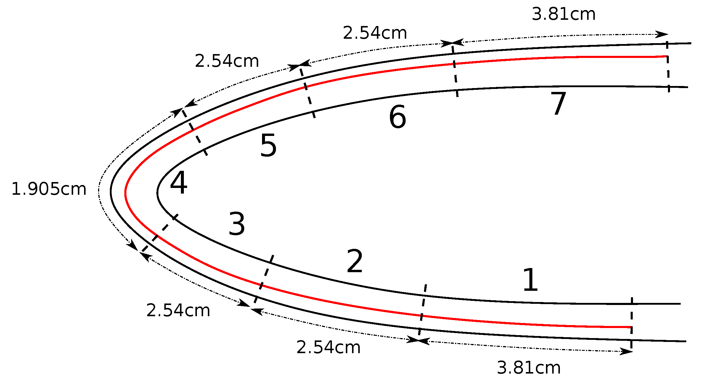
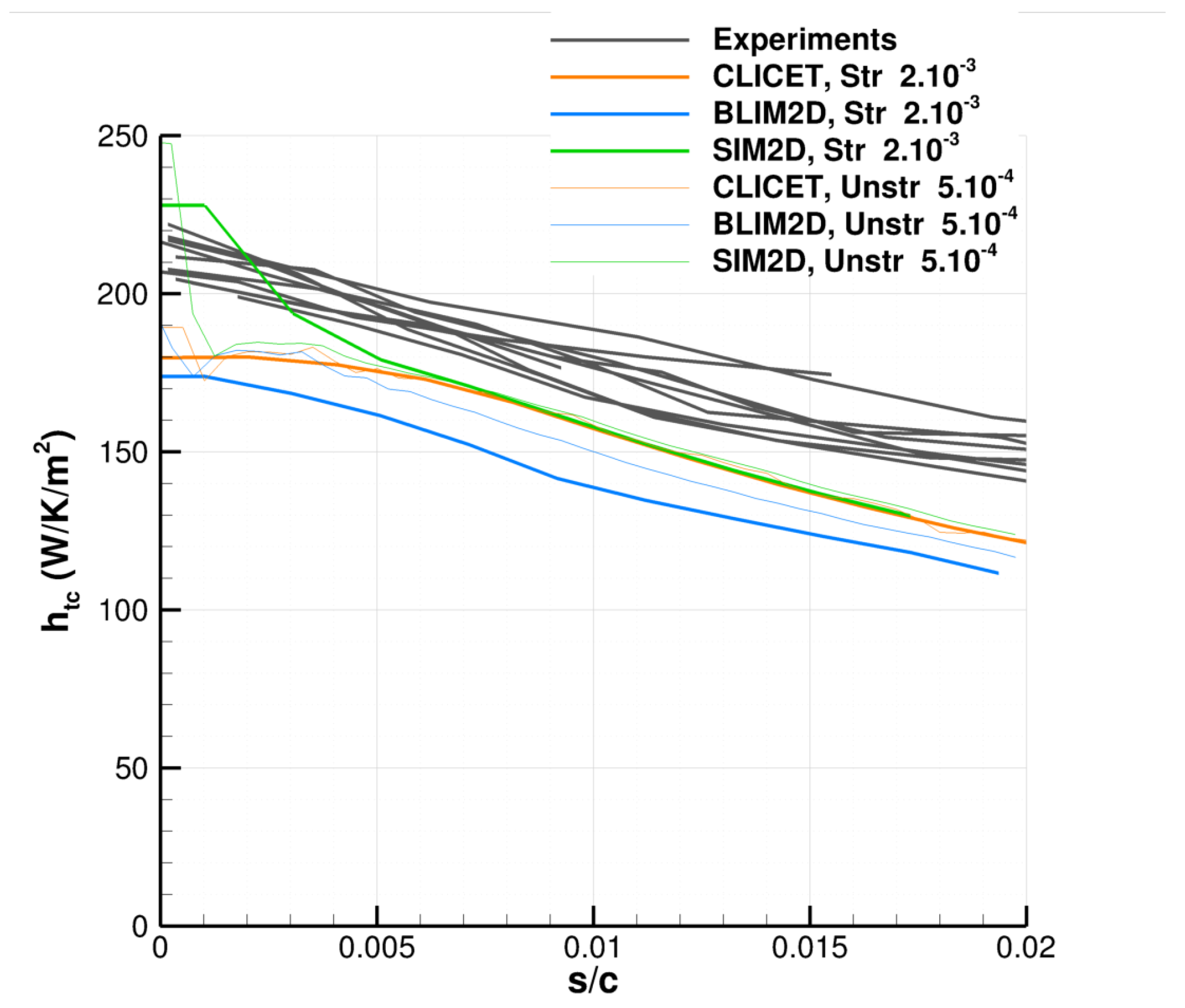
The experimental conditions are as follows: a NACA0012 airfoil, whose chord length is c = 0.5334 m, was put in a wind tunnel. The aerodynamic flow has an upstream velocity of about V 35 m/s, the outside air temperature is about T 295 K, while the wall temperature is about T w 298 K. The experimental data are unfortunately known approximately. The measurements of h t c have been digitized, and more precisely, they have been reconstructed from the graphs of Frossling number Fr = h t c × c λ Re 0.5 , where the air conductivity λ was taken equal to 2.2 × 10 2 W/m/K and the Reynolds number is Re = P c V r T μ ( r = 287 J/K/kg for air, μ is given by the Sutherland law, and the pressure was set to P = 93,000 Pa here).
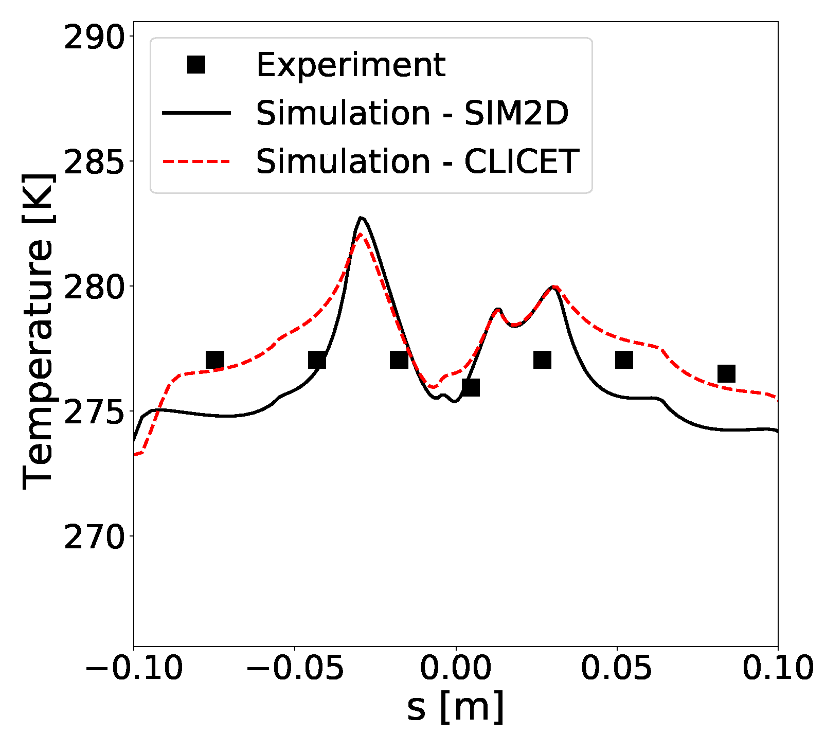
Despite the low precision of the input data, the agreement on h t c between the codes and the experimental data is rather good. The experimental data set has been plotted in Figure A1 for different roughness sizes. As expected, the roughness size affects only the extent of the laminar area, and the values of h t c coincide rather well for all sets of measurements.
Figure A1. Solution produced by CLICET, SIM2D, and BLIM2D for the heat transfer coefficient with respect to the curvilinear abscissa s in the laminar area of Han and Palacios’s experiment for several meshes. Comparison against the experimental measurements.
Aerospace 10 00075 g0a1
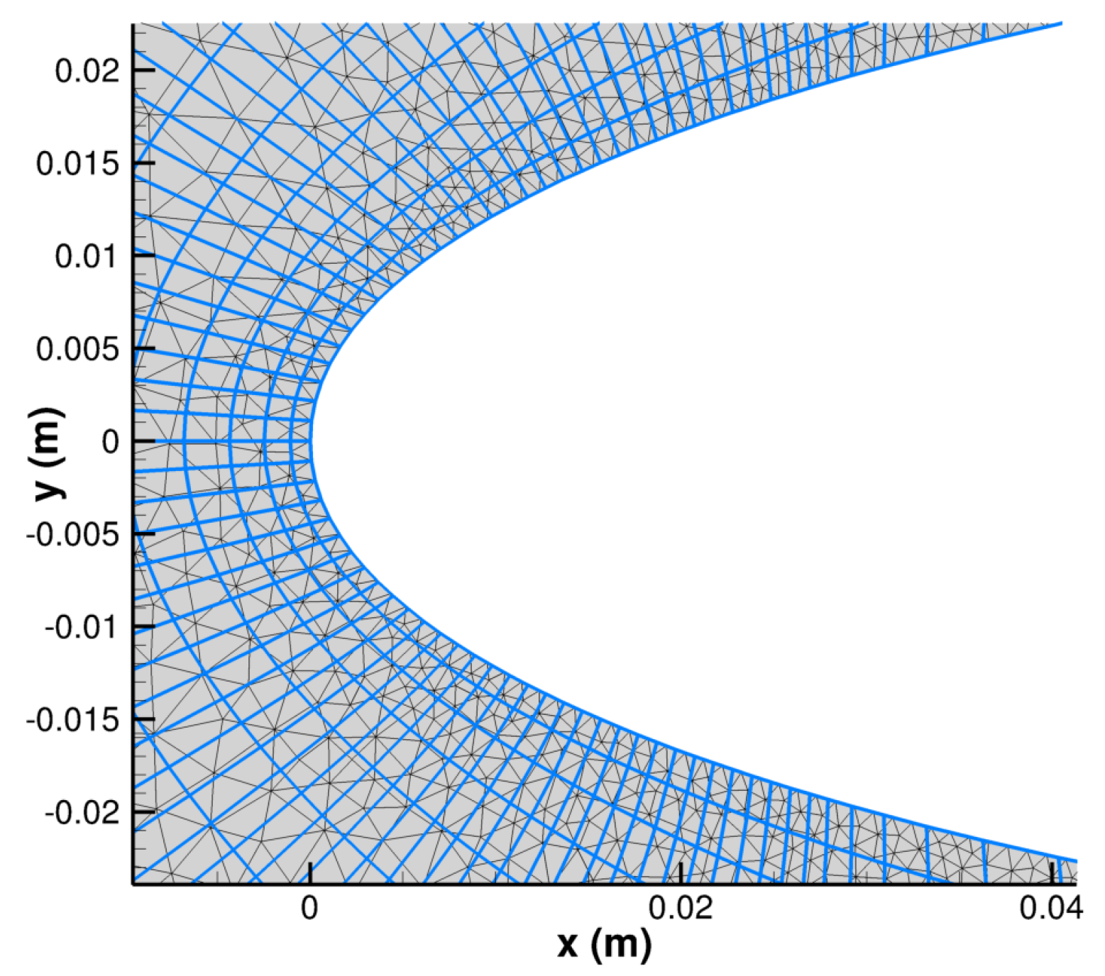
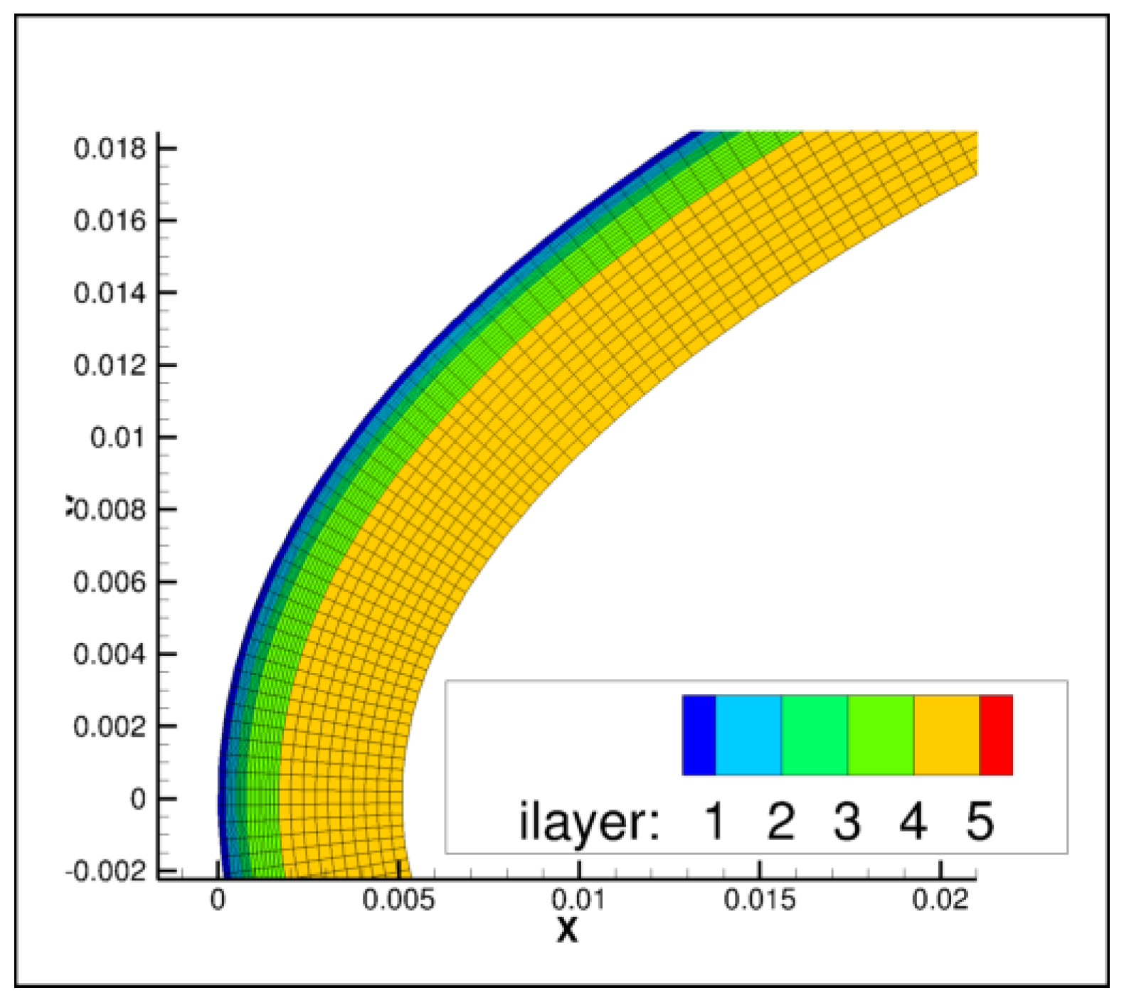
For the simulations, several meshes were used. The first mesh is the default structured mesh of IGLOO2D [11]. The others are unstructured meshes of different refinement levels. The structured mesh is rather refined around the leading edge of the airfoil (Figure A2), where the mesh size is around Δ x L E 2 × 10 3 × c . Further downstream, the mesh is coarsened, especially downstream of the first five percent of the chord length, the mesh size reaching around 0.05 × c in the downstream half of the airfoil. Figure A2 shows that the mesh size is more uniform for the unstructured meshes, here on the example of the coarsest mesh for which the same level of refinement is used at the leading edge as for the structured mesh. Two additional levels of refinement were employed for these unstructured meshes, two times ( Δ x L E 1 × 10 3 × c ) and four times ( Δ x L E 5 × 10 4 × c ) finer than the coarse mesh, respectively.
Figure A2. Meshes used for the simulation of the Han and Palacios test case. Default structured mesh in blue lines, coarsest unstructured mesh in black lines.
Aerospace 10 00075 g0a2
As in Section 4.4, inviscid simulations were performed with the solver EULER2D. The boundary-layer solution was then computed with the three solvers presented earlier, CLICET, BLIM2D, and SIM2D, fed with the inviscid solution. For these simulations, the laminar area was maintained up to the non-dimensional abscissa s / c = 0.02 . The simulations with the intermediate unstructured mesh ( Δ x L E 1 × 10 3 × c ) are not shown in the following figures because the results are very close to those of the finest mesh ( Δ x L E 5 × 10 4 × c ), except for the region near the stagnation point ( s = 0 
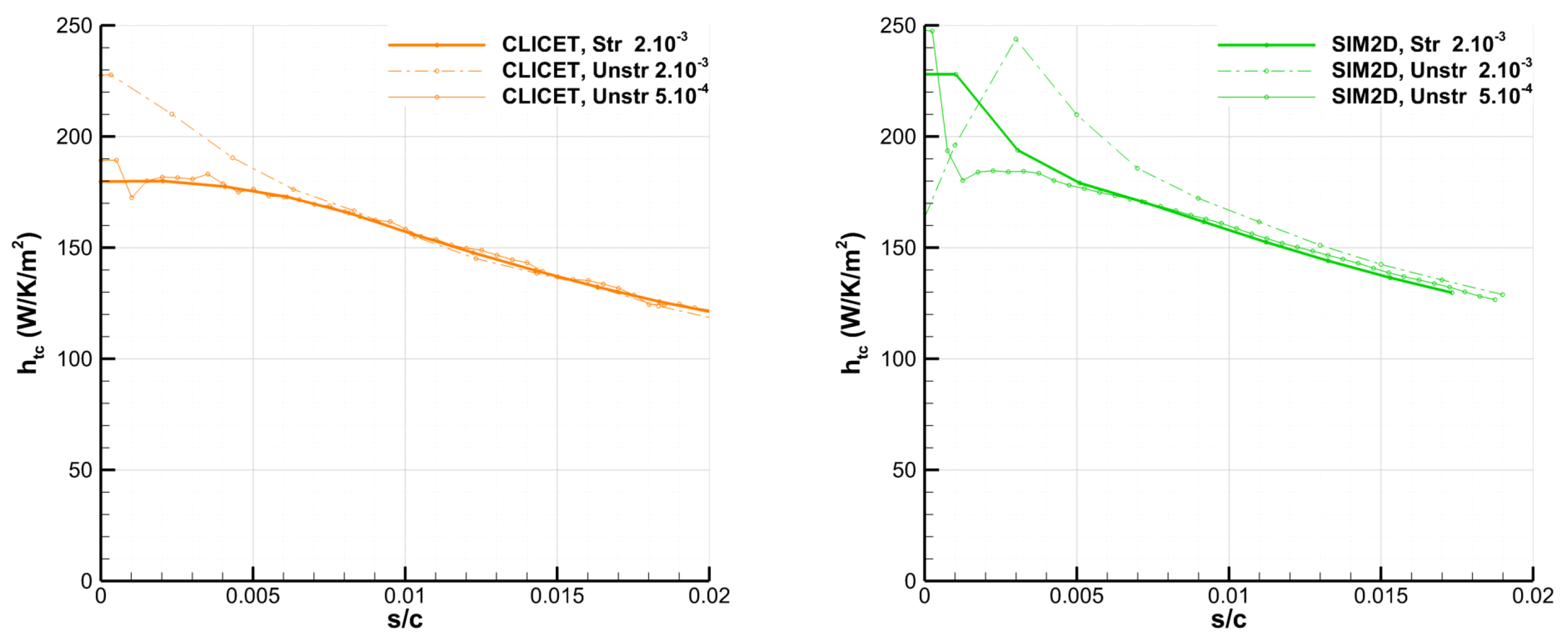
) showing that mesh convergence is achieved. The simulation with CLICET captures quite well the experimental data, taking into account the uncertainties of the experimental inputs (Figure A1). In addition, Figure A3 (left) shows that all the meshes produce very similar solutions, except in the vicinity of the stagnation point, which is more difficult to capture and requires sufficient mesh refinement and quality. The SIM2D solution, which is fed with the same inviscid data from EULER2D, is only slightly more sensitive to mesh convergence than CLICET (Figure A3, right), and the solution is very good compared to the experiments too (Figure A1), which justifies even more the use of this type of solver for unheated applications. For this, however, it was necessary to correct h t c in the following way:
h t c = h S T w T r e c T w T ,
because the heat transfer coefficient h S of SIM2D is used as Φ w = h S T w T r e c , where T r e c is the recovery temperature. Moreover, it is worth noting that SIM2D only slightly overstimates h t c compared to CLICET in the immediate vicinity of s = 0 .
Figure A3. Solution produced by CLICET and SIM2D for the heat transfer coefficient in the laminar area of Han and Palacios’s experiment for several meshes. (Left): CLICET solution. (Right): SIM2D solution.
Aerospace 10 00075 g0a3
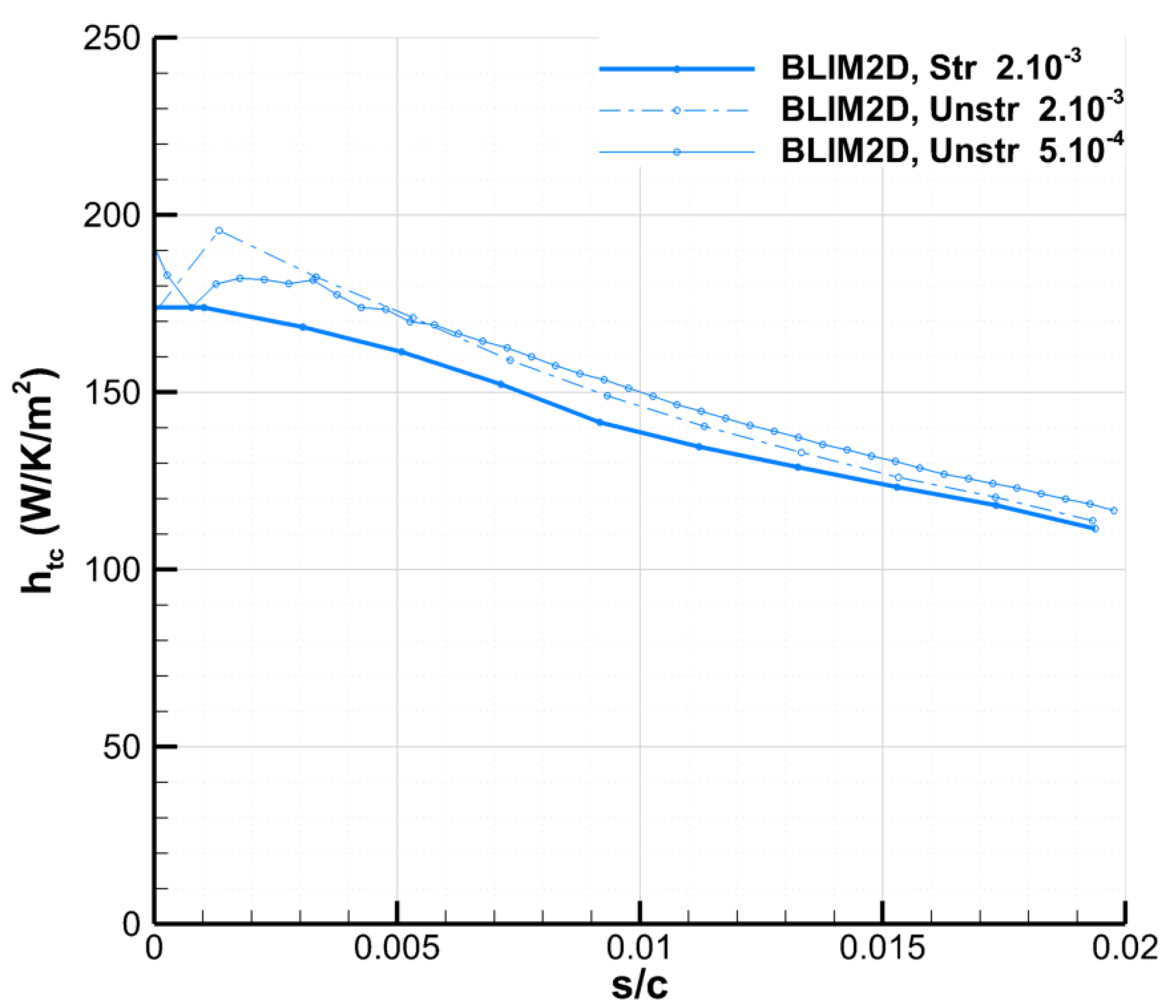
The simulation with BLIM2D, also fed with the same EULER2D data, slightly underestimates h t c , but the error is rather small (Figure A1). However, the sensitivity to the mesh is larger than for the other solvers, as shown in Figure A4. The standard structured mesh is indeed not fine enough and slightly underestimates h t c all along the profile. To sum up, for sufficiently fine meshes, the difference between the results of the three codes is very small (Figure A1). The main difference is finally that SIM2D overestimates h t c near s = 0 , which is a particularly tricky region to capture with this code.
Figure A4. Solution produced by BLIM2D for the heat transfer coefficient in the laminar area of Han and Palacios’s experiment for several meshes.
Aerospace 10 00075 g0a4
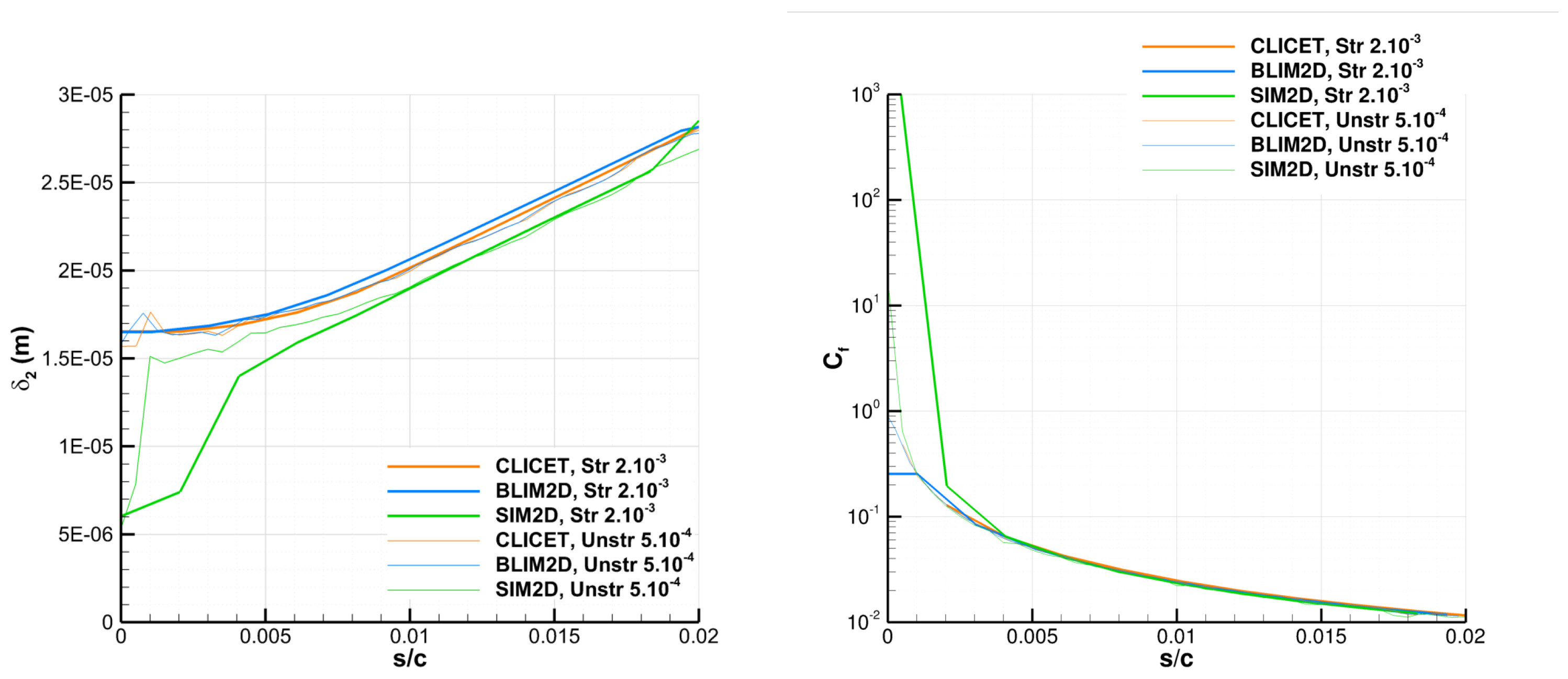
In addition, regarding other classical data of boundary-layer approaches, the agreement is very good between BLIM2D and CLICET on the momentum thickness δ 2 and the skin friction coefficient C f , as shown in Figure A5. In addition, BLIM2D’s sensitivity to the mesh is weaker than for h t c for these dynamic boundary-layer parameters. SIM2D is less accurate for these two variables compared to CLICET (although still providing a rather good approximation), which highlights the lack of generality of the approach.
Figure A5. Solution produced by CLICET, BLIM2D, and SIM2D for the momentum thickness and the skin friction coefficient in the laminar area of Han and Palacios’s experiment for several meshes. (Left): δ 2 . (Right): C f .
Aerospace 10 00075 g0a5

Appendix A.2. Simulations on an Airfoil with Uniform Wall Temperature

For further analysis, comparisons between CLICET, BLIM2D, and SIM2D are performed on the cases of Bayeux’s article [34] (Table A1), for which the dynamic boundary layer has already been studied in detail by Bayeux et al. All simulations are again performed by feeding the different boundary-layer codes with the velocity fields computed by the inviscid code EULER2D. In this section, a brief reminder is given on the accuracy of the results obtained for the dynamic boundary layer in Case 1 of Table A1, with CLICET as the reference. Concerning the thermal boundary layer, the convective heat transfer coefficient h t c is the key result. There is no ambiguity about the calculation method for the simplified SIM2D method (see Section 4.3, Equation (18)). However, both CLICET and BLIM2D perform a heat flux calculation for an imposed wall temperature. In practice, for these two codes, the heat transfer coefficient is thus derived from the linearization:
h t c = Φ w 2 Φ w 1 T w 2 T w 1 ,
where T w 1 and T w 2 are, respectively, the two wall temperatures imposed for two different simulations, Φ w 2 and Φ w 1 are the wall heat fluxes produced for each of these simulations. For CLICET, T w 1 = T r e c 5 K and T w 2 = T r e c + 5 K [35]. For BLIM2D, as the method does not allow simulating cooled walls, T w 1 = T r e c + 5 K and T w 2 = T r e c + 10 K [35]. It has been verified in Bayeux’s Ph.D. thesis [35] that the impact of the choice of T w 1 and T w 2 is small (in particular by using T w 1 = T r e c + 5 K and T w 2 = T r e c + 10 K for CLICET on some cases).
Table A1. Test cases for the analysis of the boundary-layer solvers.
CaseProfilec (m)AOA ( ) M T (K) P (Pa)
Case 1NACA00120.50040.3026380,000
Case 2NACA00120.50000.1526380,000
Case 3MS3170.91400.2420263101,325
Case 4MS3170.91480.2420263101,325
Case 5GLC3050.91444.50.2730268.30101,325
Case 6GLC3050.91441.50.3940263.60101,325
Cases 1 and 2 of Table A1 are NACA0012 airfoils for which the Vassberg and Jameson meshes were used [51]. In Case 2 of Table A1 in particular, it was shown that the mesh composed of 1024 points on the surface of the airfoil ensures mesh convergence [
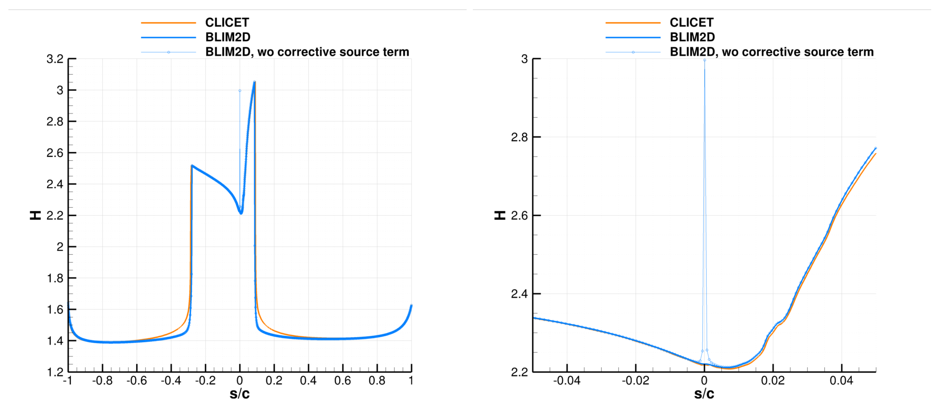
34]. Therefore, this mesh was used here for Case 1 as well. To first address the results of the dynamic boundary layer, Figure A6 (left) shows that the shape factor H = δ 1 / δ 2 is well reproduced by BLIM2D, compared to CLICET. Figure A6 (right) shows the interest in introducing a corrective source term for the numerical issue faced at the stagnation point ( s = 0 ), which was shown in Case 2 in Bayeux’s article [34]. This source term corrects a significant error in H, and it affects only the immediate vicinity of s = 0 
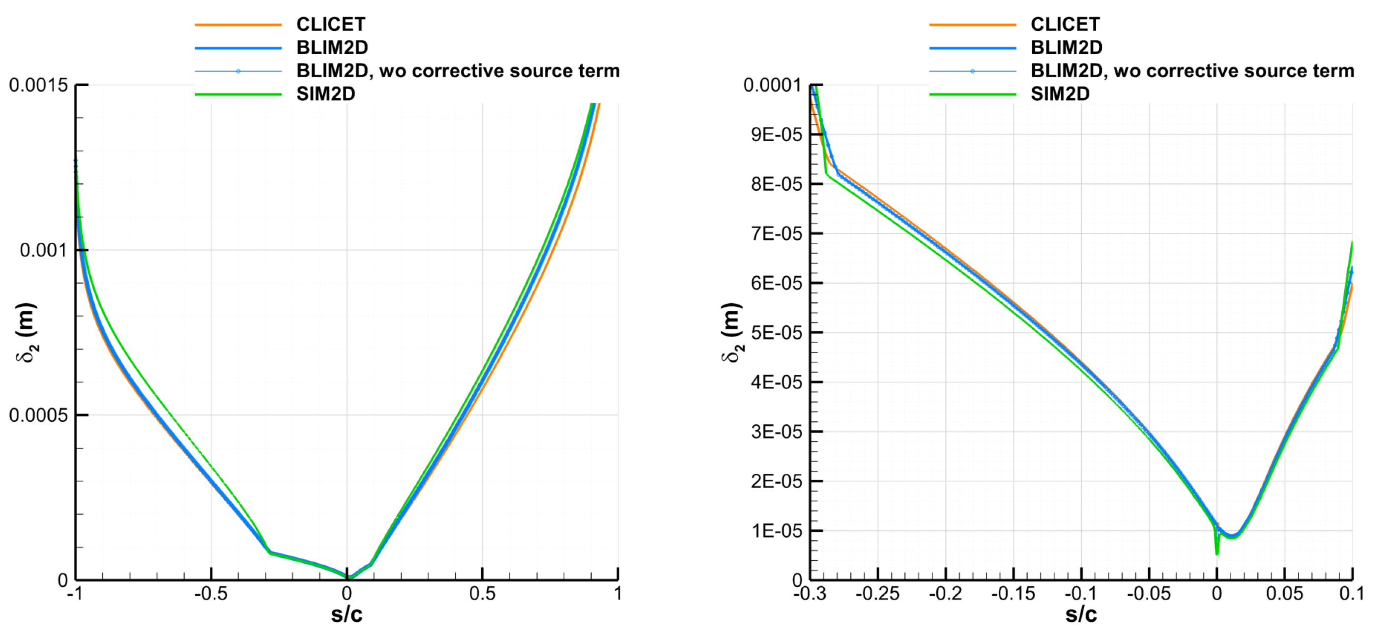
. It also affects the dynamic integral thicknesses, such as the momentum thickness δ 2 (Figure A7, right). Regarding δ 2 , 
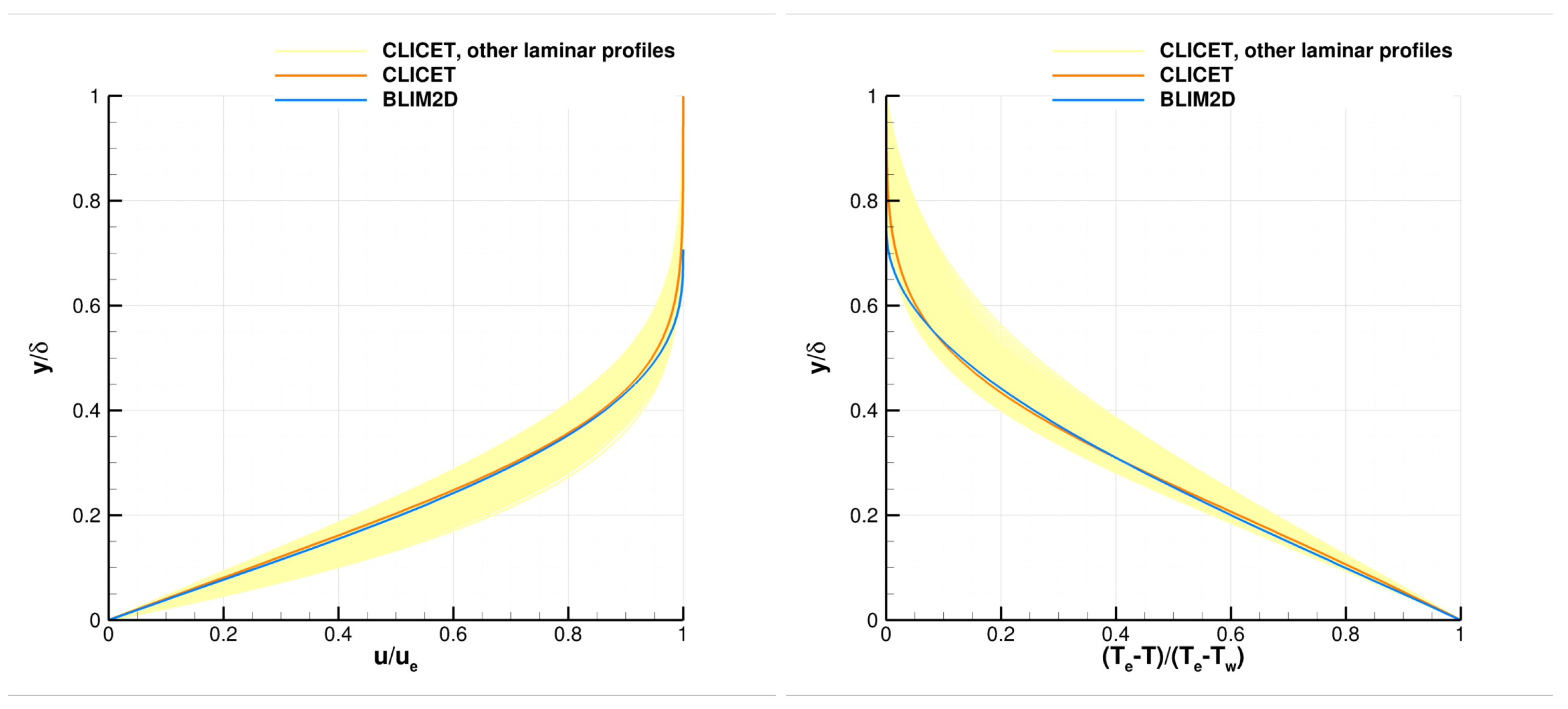
Figure A7 (left) shows that BLIM2D captures very well the evolution predicted by CLICET in the laminar area ( s / c in the range between −0.3 and 0.1), especially on pressure side ( s / c < 0 ). The results are still very good outside this area but a little less accurate. The simplified SIM2D method produces slightly worse results.
Figure A6. Solution produced by CLICET and BLIM2D for the shape factor H in Case 1 of Table A1. (Left): whole airfoil. (Right): focus in the vicinity of the stagnation point.
Aerospace 10 00075 g0a6
Figure A7. Solution produced by CLICET, SIM2D, and BLIM2D for the momentum thickness δ 2 in Case 1 of Table A1. (Left): whole airfoil. (Right): laminar area.
Aerospace 10 00075 g0a7
The resolution of the thermal boundary layer does not suffer from the issue identified at the stagnation point for the dynamic boundary layer (which is related to the fact that the numerical flux term evolves linearly with respect to u e and that the issue comes from discretization errors of derivatives of u e n terms present in the flux terms, with exponents n larger than one, as shown in Bayeux’s article [34]). 
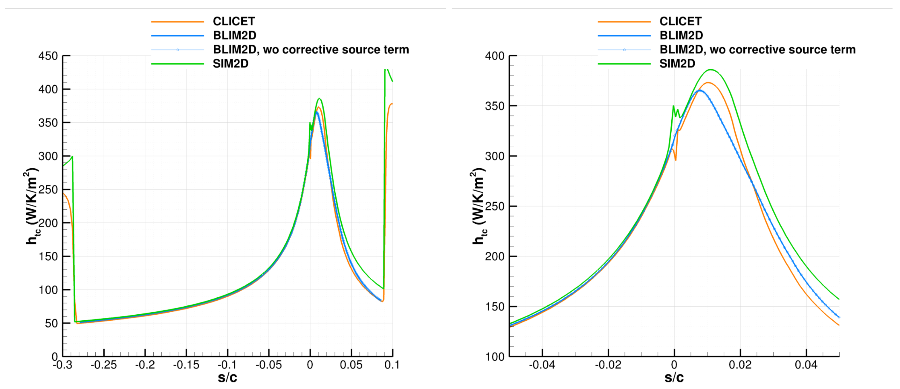
Figure A8 (right) indeed shows that h t c 
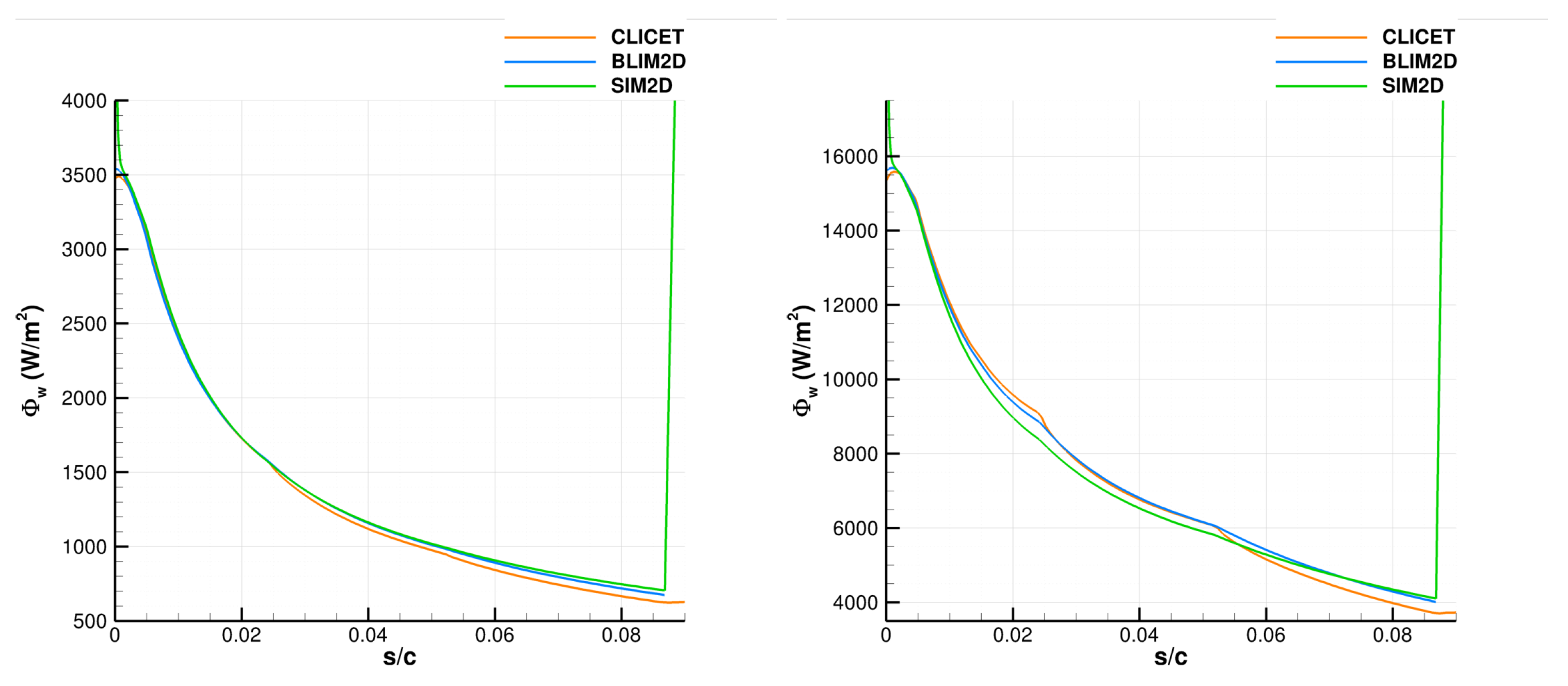
is the same whether the corrective source term is activated or not. This area is even simulated more smoothly than for CLICET. Moreover, Figure A8 (left) shows the very good agreement between BLIM2D and CLICET on h t c in the whole laminar area. The BLIM2D method for the thermal boundary layer was developed for the laminar regime only, so the comparison is limited to this region. The SIM2D solution is quite correct, which justifies the widespread use of such simplified approaches for ice-accretion calculations. However, the BLIM2D solution is rather better at the stagnation point for the maximum value of h t c (in the accelerated area of the suction side of the airfoil) and on the suction side in general.
Figure A8. Solution produced by CLICET, SIM2D, and BLIM2D for the convective heat transfer coefficient h t c in Case 1 of Table A1. (Left): laminar area. (Right): focus in the vicinity of the stagnation point.
Aerospace 10 00075 g0a8
Regarding the other cases of Table A1, the same observations are made concerning h t c . Table A2 indeed shows that the average error (relative error L 2 , compared to CLICET) in the laminar region is indeed systematically higher for SIM2D, reaching almost 0.1 for Case 6, while it is limited to around 0.05 for BLIM2D (Cases 4, 5, and 6). The error at the stagnation point is even higher. With the exception of Case 4 for which the CLICET solution is oscillating near s = 0 . the error made by SIM2D is indeed again systematically larger (in general significantly) than for BLIM2D.
Table A2. Relative errors in h t c in the laminar area for the six cases of Table A1. L2-norm relative error ε 2 = h t c h t c , CLICET 2 / h t c 2 . Relative error at the stagnation point ε S P = h t c ( s = 0 ) h t c , CLICET ( s = 0 ) / h t c , CLICET ( s = 0 ) .
Case ε 2 , BLIM 2 D ε 2 , SIM 2 D ε SP , BLIM 2 D ε SP , SIM 2 D
Case 10.04000.07290.03020.1445
Case 20.01570.05680.02270.2813
Case 30.01320.04500.04860.1461
Case 40.05280.06680.20470.0384
Case 50.04630.06620.05490.1476
Case 60.05400.09650.07420.1476
Even if SIM2D can capture these cases well, BLIM2D reduces the error on h t c , even for these very simple cases where the wall has a nearly constant temperature.

Appendix B. ETIPS Mesh Information

The mesh used to solve the heat equation inside the electrothermal ice protection system was composed of 10,000 cells. As shown in Figure A10, this discretization provides sufficiently converged results for the targeted applications. The mesh was generated in a structured way by discretizing each layer and each zone of the outer boundary with a given number of cells (see Table A3 and Table A4 for details). A close-up view of the mesh is shown in Figure A9.
Figure A9. Mesh of the electrothermal system in the upper part of the leading edge.
Aerospace 10 00075 g0a9
Figure A10. Comparison between results obtained with 2 meshes (10,000 cells and 20,000 cells) during the last 3 cycles.
Aerospace 10 00075 g0a10
Table A3. Thickness and discretization of the multilayered stack.
LayerThickness [mm]nb. Cells
10.204
20.28656
30.28656
40.898
53.4310
Table A4. Definition of zones in terms of starting ( s 1 ) and ending ( s 2 ) curvilinear abscissa and the associated discretization.
Zone s 1 [m] s 2 [m]nb. Cells
1−0.2−0.09885315
2−0.098853−0.05575330
3−0.055753−0.03035330
4−0.030353−0.00495340
5−0.0049530.01409740
60.0140970.03949740
70.0394970.06489730
80.0648970.10299730
90.1029970.215

References

  1. Henry, R. Development of an Electrothermal De-icing/Anti-icing Model. In Proceedings of the AIAA 30th Meeting, Reno, NV, USA, 6–9 January 1992. [Google Scholar] [CrossRef]
  2. Wright, W.; Dewitt, K.; Keith, T., Jr. Numerical Simulation of Icing, Deicing and Shedding. In Proceedings of the 29th Aerospace Sciences Meeting, Reno, NV, USA, 7–10 January 1991. AIAA-91-0665. [Google Scholar]
  3. Huang, X.; Tepylo, N.; Pommier-Budinger, V.; Budinger, M.; Bonaccurso, E.; Villedieu, P.; Bennani, L. A survey of icephobic coatings and their potential use in a hybrid coating/active ice protection system for aerospace applications. Prog. Aerosp. Sci. 2019, 105, 74–97. [Google Scholar] [CrossRef] [Green Version]
  4. He, Z.; Xie, H.; Jamil, M.I.; Li, T.; Zhang, Q. Electro-/Photo-Thermal Promoted Anti-Icing Materials: A New Strategy Combined with Passive Anti-Icing and Active De-Icing. Adv. Mater. Interfaces 2022, 9, 2200275. [Google Scholar] [CrossRef]
  5. Messinger, B.L. Equilibrium Temperature of an Unheated Icing Surface as a Function of Air Speed. J. Aeronaut. Sci. 1953, 20, 29–42. [Google Scholar] [CrossRef]
  6. Gent, R.W. TRAJICE2–A combined water droplet trajectory and ice accretion prediction program for aerofoils. RAE TR 1990, 90054. [Google Scholar]
  7. Dillingh, J.E.; Hoeijmakers, H.W.M. Simulation of Ice Accretion on Airfoils during Flight. In Proceedings of the FAA In-Flight Icing/Ground De-Icing International Conference and Exhibition 2003, Chicago, IL, USA, 16–20 June 2003; Technical Report; SAE Technical Paper. SAE: Warrendale, PA, USA, 2003. [Google Scholar]
  8. Hedde, T.; Guffond, D. ONERA three-dimensional icing model. AIAA J. 1995, 33, 1038–1045. [Google Scholar] [CrossRef]
  9. Paraschivoiu, I.; Saeed, F. Ice accretion simulation code canice. In Proceedings of the International Aerospace Symposium Carafoli, Bucharest, Romania, 19–20 October 2001; pp. 81–86. [Google Scholar]
  10. Wright, W. User’s Manual for LEWICE Version 3.2; NASA/CR–2008-214255; National Aeronautics and Space Administration: Washington, DC, USA, 2008. [Google Scholar]
  11. Trontin, P.; Blanchard, G.; Kontogiannis, A.; Villedieu, P. Description and assessment of the new ONERA 2D icing suite IGLOO2D. In Proceedings of the 9th AIAA Atmospheric and Space Environments Conference, Denver, CO, USA, 5–9 June 2017. AIAA 2017-3417. [Google Scholar]
  12. Bourgault, Y.; Beaugendre, H.; Habashi, W. Development of a shallow-water icing model in FENSAP-ICE. J. Aircr. 2000, 37, 640–646. [Google Scholar] [CrossRef]
  13. Otta, S.; Rothmayer, A. Instability of stagnation line icing. Comput. Fluids 2009, 38, 273–283. [Google Scholar] [CrossRef]
  14. de Segura Solay, G.G.; Radenac, E.; Chauvin, R.; Laurent, C. Simulations of ice accretion, runback and droplet re-emission in a multi-stage model of aeronautical engine. In Proceedings of the 8th AIAA Atmospheric and Space Environments Conference, Washington, DC, USA, 13–17 June 2016. AIAA 2016-4350. [Google Scholar]
  15. Verdin, P.; Charpin, J.; Thompson, C. Multistep Results in ICECREMO2. J. Aircr. 2009, 46, 1607–1613. [Google Scholar] [CrossRef]
  16. Lavoie, P.; Bourgault-Côté, S.; Laurendeau, E. Numerical algorithms for infinite swept wing ice accretion. Comput. Fluids 2018, 161, 189–198. [Google Scholar] [CrossRef]
  17. Myers, T.; Hammond, D. Ice and water film growth from incoming supercooled droplets. Int. J. Heat Mass Transf. 1999, 42, 2233–2242. [Google Scholar] [CrossRef]
  18. Myers, T.G. Extension to the messinger model for aircraft icing. AIAA J. 2001, 39, 211–218. [Google Scholar] [CrossRef] [Green Version]
  19. Yanxia, D.; Yewei, G.; Chunhua, X.; Xian, Y. Investigation on heat transfer characteristics of aircraft icing including runback water. Int. J. Heat Mass Transf. 2010, 53, 3702–3707. [Google Scholar] [CrossRef]
  20. Gori, G.; Zocca, M.; Garabelli, M.; Guardone, A.; Quaranta, G. PoliMIce: A simulation framework for three-dimensional ice accretion. Appl. Math. Comput. 2015, 267, 96–107. [Google Scholar] [CrossRef]
  21. Myers, T.; Mitchell, S.; Muchatibaya, G.; Myers, M. A cubic heat balance integral method for one-dimensional melting of a finite thickness layer. Int. J. Heat Mass Transf. 2007, 50, 5305–5317. [Google Scholar] [CrossRef]
  22. Chauvin, R.; Bennani, L.; Trontin, P.; Villedieu, P. An implicit time marching Galerkin method for the simulation of icing phenomena with a triple layer model. Finite Elem. Anal. Des. 2018, 150, 20–33. [Google Scholar] [CrossRef] [Green Version]
  23. Bennani, L.; Trontin, P.; Chauvin, R.; Villedieu, P. A non-overlapping optimized Schwarz method for the heat equation with non linear boundary conditions and with applications to deicing. Comput. Math. Appl. 2020, 80, 1500–1522. [Google Scholar] [CrossRef]
  24. Croce, G.; Beaugendre, H.; Habashi, W. CHT3D—FENSAP-ICE conjugate heat transfer computations with droplet impingement and runback effects. In Proceedings of the 40th AIAA Aerospace Sciences Meeting and Exhibit, Reno, NV, USA, 14–17 January 2002. [Google Scholar] [CrossRef]
  25. Bu, X.; Lin, G.; Shen, X.; Hu, Z.; Wen, D. Numerical simulation of aircraft thermal anti-icing system based on a tight-coupling method. Int. J. Heat Mass Transf. 2020, 148, 119061. [Google Scholar] [CrossRef]
  26. Morency, F.; Tezok, F.; Paraschivoiu, I. Anti-icing system simulation using CANICE. J. Aircr. 1999, 36, 999–1006. [Google Scholar] [CrossRef]
  27. Al-Khalil, K.; Horvath, C.; Miller, D.; Wright, W. Validation of NASA thermal ice protection computer codes. III–The validation of ANTICE. In Proceedings of the 35th Aerospace Sciences Meeting and Exhibit, Reno, NV, USA, 6–9 January 1997. [Google Scholar] [CrossRef]
  28. da Silva, G.A.L.; de Mattos Silvares, O.; de Jesus Zerbini, E.J.G. Numerical Simulation of Airfoil Thermal Anti-Ice Operation. Part 1: Mathematical Modeling. J. Aircr. 2007, 44, 627–633. [Google Scholar] [CrossRef]
  29. Bu, X.; Lin, G.; Yu, J.; Yang, S.; Song, X. Numerical simulation of an airfoil electrothermal anti-icing system. Proc. Inst. Mech. Eng. Part G J. Aerosp. Eng. 2013, 227, 1608–1622. [Google Scholar] [CrossRef]
  30. Chauvin, R.; Villedieu, P.; Trontin, P. A robust coupling algorithm applied to thermal ice protection system unsteady modeling. In Proceedings of the 6th AIAA Atmospheric and Space Environments Conference, Atlanta, GA, USA, 16–20 June 2014. AIAA 2014-2061. [Google Scholar]
  31. Morency, F.; Tezok, F.; Paraschivoiu, I. Heat and Mass Transfer in the Case of Anti-Icing System Simulation. J. Aircr. 2000, 37, 245–252. [Google Scholar] [CrossRef]
  32. Kays, W.; Crawford, M. Convective Heat and Mass Transfer; McGraw-Hill: New York, NY, USA, 1993. [Google Scholar]
  33. Aupoix, B. Couches Limites Bidimensionnelles Compressibles. Descriptif et Mode d’emploi du Code CLICET–Version 2015; Technical Report; ONERA: Palaiseau, France, 2015. [Google Scholar]
  34. Bayeux, C.; Radenac, E.; Villedieu, P. Theory and Validation of a 2D Finite-Volume Integral Boundary-Layer Method for Icing Applications. AIAA J. 2019, 57, 1092–1112. [Google Scholar] [CrossRef]
  35. Bayeux, C. Méthode Intégrale pour la Couche Limite Tridimensionnelle. Applications au Givrage. Ph.D. Thesis, Institut Superieur De l’Aeronautique Et De L’Espace (ISAE), Toulouse, France, 2017. [Google Scholar]
  36. Radenac, E.; Kontogiannis, A.; Bayeux, C.; Villedieu, P. An extended rough-wall model for an integral boundary-layer model intended for ice accretion calculations. In Proceedings of the 10th AIAA Atmospheric and Space Environments Conference–AVIATION 2018, Atlanta, GA, USA, 25–29 June 2018. AIAA 2018-2858. [Google Scholar] [CrossRef]
  37. Radenac, E. Validation of a 3D ice accretion tool on swept wings of the SUNSET2 program. In Proceedings of the 8th AIAA Atmospheric and Space Environments Conference, Washington, DC, USA, 13–17 June 2016. AIAA 2016-3735. [Google Scholar]
  38. Chauvin, R. Un Modèle Unifié Pour Les Phénomènes De Givrage en Aéronautique et Les Systèmes De Protection Thermiques. Ph.D. Thesis, ISAE, Toulouse, France, 2015. [Google Scholar]
  39. Chilton, T.H.; Colburn, A.P. Mass transfer (absorption) coefficients prediction from data on heat transfer and fluid friction. Ind. Eng. Chem. 1934, 26, 1183–1187. [Google Scholar] [CrossRef]
  40. Cousteix, J. Aérodynamique et Couche Limite Laminaire; Cepadues: Toulouse, France, 1989. [Google Scholar]
  41. Aupoix, B. Roughness corrections for the k-ω shear stress transport model: Status and proposals. J. Fluids Eng. 2015, 137, 021202. [Google Scholar] [CrossRef]
  42. Chedevergne, F. Analytical wall function including roughness corrections. Int. J. Heat Fluid Flow 2018, 73, 258–269. [Google Scholar] [CrossRef] [Green Version]
  43. Cebeci, T.; Cousteix, J. Modeling and Computation of Boundary-Layer Flows; Springer: New York, NY, USA, 1999. [Google Scholar]
  44. Spalart, P.; Allmaras, S. A one-equation turbulence model for aerodynamic flows. In Proceedings of the 30th Aerospace Sciences Meeting and Exhibit, Reno, NV, USA, 6–9 January 1992. AIAA 1992-439. [Google Scholar]
  45. Drela, M. MISES Implementation of Modified Abu-Ghannam/Shaw Transition Criterion; Technical Report. 1998. Available online: https://web.mit.edu/drela/Public/web/mises/ags2.pdf (accessed on 9 January 2023).
  46. Menter, F.R. Two-equation eddy-viscosity turbulence models for engineering applications. AIAA J. 1994, 32, 1598–1605. [Google Scholar] [CrossRef] [Green Version]
  47. Bempedelis, N.; Bayeux, C.; Blanchard, G.; Radenac, E.; Villedieu, P. A 3D Finite-Volume Integral Boundary Layer method for icing applications. In Proceedings of the 9th AIAA Atmospheric and Space Environments Conference–AVIATION 2017, Denver, CO, USA, 5–9 June 2017. AIAA 2017-3419. [Google Scholar] [CrossRef]
  48. Blanchard, G.; Radenac, E.; Bempedelis, N.; Bayeux, C.; Villedieu, P. 3D ice accretion modeling using an integral boundary-layer method. In Proceedings of the 7th European Conference for Aeronautics and Aerospace Sciences (EUCASS), EUCASS 2017-400, Milan, Italy, 3–6 July 2017. [Google Scholar] [CrossRef]
  49. Smith, A.; Spalding, D. Heat transfer in a laminar boundary-layer with constant fluid properties and constant wall temperature. J. R. Aeronaut. Soc. 1958, 62, 60–64. [Google Scholar] [CrossRef]
  50. Ambrok, G.S. Approximate solutions of equations for the thermal boundary layerwith variations in the boundary-layer structure. Sov. Phys. Tech. Phys. 1957, 2, 1979–1986. [Google Scholar]
  51. Vassberg, J.C.; Jameson, A. In Pursuit of Grid Convergence for Two-Dimensional Euler Solutions. J. Aircr. 2010, 47, 1152–1166. [Google Scholar] [CrossRef] [Green Version]
  52. Harry, R.; Radenac, E.; Blanchard, G.; Villedieu, P. Heat Transfer modeling by integral boundary-layer methods towards icing applications. In Proceedings of the AIAA Aviation 2021 Forum, Virtual Event, 2–6 August 2021. [Google Scholar] [CrossRef]
  53. Radenac, E.; Harry, R.; Villedieu, P. A Galerkin Method for the Simulation of Laminar Boundary Layers on Heated Walls. Energies 2022, 15, 3267. [Google Scholar] [CrossRef]
  54. Wright, W.; Al-Khalil, K.; Miller, D. Validation of NASA thermal ice protection computer codes. II-LEWICE/Thermal. In Proceedings of the 35th Aerospace Sciences Meeting and Exhibit, Reno, NV, USA, 6–9 January 1997. AIAA 1997-50. [Google Scholar]
  55. Arizmendi, B.; Morelli, M.; Parma, G.; Zocca, M.; Quaranta, G.; Guardone, A. In-Flight Icing: Modeling, Prediction, and Uncertainty; Springer: New York, NY, USA, 2021; pp. 455–506. [Google Scholar]
  56. Gori, G.; Congedo, P.M.; Le Maître, O.; Bellosta, T.; Guardone, A. Modeling in-flight ice accretion under uncertain conditions. J. Aircr. 2022, 59, 799–813. [Google Scholar] [CrossRef]
  57. Han, Y.; Palacios, J. Surface roughness and heat transfer improved predictions for aircraft ice-accretion modeling. AIAA J. 2017, 55, 1318–1331. [Google Scholar] [CrossRef]
  58. Han, Y. Aerodynamics and Thermal Physics of Helicopter Ice Accretion. Ph.D. Thesis, Pennsylvania State University, State College, PA, USA, 2015. [Google Scholar]
Figure 1. Operating of an ETIPS.
Aerospace 10 00075 g001
Figure 2. Illustration of the different physical phenomena taking place when an electrothermal ice protection system is being operated.
Aerospace 10 00075 g002
Figure 3. The architecture of the IGLOO2D icing suite developed at ONERA. The work presented in this article focuses on the computation of the boundary layer, the ice accretion solver, and the heat conduction solver.
Aerospace 10 00075 g003
Figure 4. Illustration of an electrothermal ice protection system. The red lines represent the heater mats.
Aerospace 10 00075 g004
Figure 5. Illustration of a generic icing situation. Reprinted from [22], ©Elsevier.
Aerospace 10 00075 g005
Figure 6. Illustration of the three layers: h f , h i , and h s are the heights of the running film, ice, and static (melted) film. The a k ’s and b k ’s represent the positions of the boundaries between each layer in the z direction (normal to the surface). Reprinted from [22], ©Elsevier.
Aerospace 10 00075 g006
Figure 7. Wall temperature in the test cases of Table 1. (Left): RUN87b. (Right): RUN22a.
Aerospace 10 00075 g007
Figure 8. Wall heat flux produced by CLICET, BLIM2D, and SIM2D in the test cases of Table 1. (Left): RUN87b. (Right): RUN22a.
Aerospace 10 00075 g008
Figure 9. Velocity and temperature profiles produced by CLICET and BLIM2D in the Test Case RUN87b of Table 1, s / c = 0.087 . (Left): velocity. (Right): temperature.
Aerospace 10 00075 g009
Figure 10. Velocity and temperature profiles produced by CLICET and BLIM2D in the Test Case RUN22a of Table 1, s / c = 0.087 . (Left): velocity. (Right): temperature.
Aerospace 10 00075 g010
Figure 11. Illustration of the layout of the studied electrothermal system.
Aerospace 10 00075 g011
Figure 12. Comparison between experimental data and numerical results for anti-icing Case 87b.
Aerospace 10 00075 g012
Figure 13. Anti-icing Case 87b: comparison between experimental data and numerical results (in the laminar region) obtained with a coupling with SIM2D, CLICET, and BLIM2D.
Aerospace 10 00075 g013
Figure 14. Comparison between experimental data and numerical results for the deicing Case.
Aerospace 10 00075 g014
Figure 15. Temperature field in the electrothermal system and unsteady ice accretion solution at different simulation times. (Top left): t = 10 s. (Top right): t = 99 s. (Bottom left): t = 110 s. (Bottom right): t = 115 s.
Aerospace 10 00075 g015
Table 1. Test cases from Al-Khalil’s database for the analysis of the boundary-layer solvers.
CaseProfilec (m)AOA ( ) M T (K) P ( Pa )
RUN87bNACA00120.914400.1376262.7100,000
RUN22aNACA00120.914400.1369265.5100,000
Table 2. Location of the heaters in terms of starting ( s 1 ) and ending ( s 2 ) curvilinear abscissas.
Heater s 1 [m] s 2 [m]
1−0.098853−0.055753
2−0.055753−0.030353
3−0.030353−0.004953
4−0.0049530.014097
50.0140970.039497
60.0394970.064897
70.0648970.102997
Table 3. Thickness and composition of the multilayered stack.
LayerMaterialThickness [mm]
1Erosion Shield0.20
2Elastomer0.2865
3Elastomer0.2865
4Fiberglass/Epoxy Composite0.89
5Silicone Foam Insulation3.43
Table 4. Material properties.
Material ρ (kg.m 3 ) c p (J.kg 1 .K 1 ) λ (W.m 1 .K 1 )
Erosion Shield8025.25502.4116.30
Elastomer1384.001256.040.256
Fiberglass/Epoxy Composite1794.061570.050.294
Silicone Foam Insulation648.751130.430.121
Table 5. Aerodynamic and icing conditions for anti-icing Case 87b.
AoA [ ] M p [Pa] T [K] LWC [g.m 3 ] MVD [ μ m]
00.137101,325262.7220
Table 6. Power densities for anti-icing Case 87b.
Heater nb1234567
Power density [W.m 2 ]3410387554257130403038753100
Table 7. Aerodynamic and icing conditions for deicing Case 1.
AoA [ ] M p [Pa] T [K] LWC [g.m 3 ] MVD [ μ m]
00.137101,325265.50.7820
Table 8. Power densities for deicing Case 1.
Heater nb1234567
Power density [W.m 2 ]12,40012,40015,500775015,50012,40012,400
Disclaimer/Publisher’s Note: The statements, opinions and data contained in all publications are solely those of the individual author(s) and contributor(s) and not of MDPI and/or the editor(s). MDPI and/or the editor(s) disclaim responsibility for any injury to people or property resulting from any ideas, methods, instructions or products referred to in the content.

